

Submitted:
14 July 2026
Posted:
15 July 2026
You are already at the latest version
Abstract
Dephosphorisation in oxygen steelmaking depends on more than the equilibrium phosphorus partition ratio. It also depends on where gas, slag, metal and injected lime powder coexist while the bath is being stirred. We develop a gas–slag–metal–particle reaction model for bottom-blown oxygen–CaO powder injection by coupling Euler–Euler transport of liquid steel, mixed slag and gas with discrete CaO-particle motion. The local source terms include oxygen dissolution, FeO/Fe2O3 conversion, CO/CO2 buffering, competitive C/Si/P oxidation, P2O5 formation, C2S–C3P fixation, reaction heat and phase-wise mass conservation. Instead of resolving every bubble or slag droplet, the model represents bubble swarms, dispersed slag and emulsified metal–slag contact through mean-field interfacial area densities tied to local phase fractions and mixing. Two cases with the same initial phosphorus content but different carbon levels are used to test reaction selectivity. In the high-carbon bath, bottom-blown oxygen is consumed first by decarburisation; the generated CO sustains plume buoyancy but reduces FeOx retention during flotation. CaO addition improves local slag formation, but it contributes to dephosphorisation only where FeOx supply, P2O5 generation and C2S–C3P fixation coincide at an active slag–metal interface. The stable dephosphorisation window therefore lies mainly in the upper slag–metal mixing zone, not in the bottom gas column. The model provides a computable basis for analysing bottom powder injection, combined blowing and low-carbon endpoint dephosphorisation in gas–slag–metal reactive flows.
Keywords:
molten-steel dephosphorisation
; gas–slag–metal reactions
; Euler–Euler–DPM modelling
; bottom-blown oxygen–CaO powder injection
1. Introduction
Phosphorus control remains one of the strictest constraints in oxygen steelmaking. Carbon, silicon, manganese, sulfur and inclusions all affect cleanliness and downstream processing, but phosphorus is especially difficult because it remains soluble in molten iron and is not removed efficiently in the reducing blast-furnace environment. Its removal is therefore shifted to oxidative steelmaking or hot-metal pretreatment, where phosphorus must be transferred into a highly basic oxidising slag[1,2,3]. Excess phosphorus increases cold brittleness, reduces toughness and narrows the processing window for low-phosphorus steels. As low-phosphorus and ultra-low-phosphorus products become more demanding, dephosphorisation has to be treated as a coupled process involving slag volume, lime consumption, iron loss, injection practice, temperature schedule and the low-carbon smelting route[3,4,5].
The equilibrium conditions for phosphorus removal are comparatively well understood. Classical work linked the phosphorus distribution ratio to oxygen potential, basicity, temperature and iron-oxide content, leading to empirical and semi-thermodynamic descriptions based on phosphorus partitioning, optical basicity, phosphorus capacity and multicomponent slag activities[2,6,7,8,9]. These studies point to a consistent requirement: high CaO activity, sufficient FeO oxygen-supply capacity, lower temperature and low activity favour transfer from metal to slag. Once a – solid solution forms, phosphorus can be fixed and the risk of rephosphorisation decreases[10,11,12,13,14,15]. CALPHAD and FactSage descriptions now cover major steelmaking-slag subsystems, including CaO–SiO2–––MgO–Al2–MnO, and can calculate multiphase equilibria among liquid slag, solid phases and gas[16,17,18,19]. The larger uncertainty is not whether phosphorus removal is thermodynamically allowed, but where that capacity is realised in a moving converter bath.
Kinetic studies have clarified many rate-controlling steps, but most of them come from laboratory systems or semi-empirical reaction models. Lime dissolution, FeO oxygen supply, metal–slag mass transfer, solid phosphate formation, slag viscosity and stirring intensity have all been examined as controls on the apparent dephosphorisation rate[10,11,12,13,14,15,20,21,22]. Those systems usually have clearer interface areas, controlled slag-to-metal ratios, more uniform temperatures and smaller flow scales than an industrial converter. In an operating bath, bubble swarms, slag droplets, metal droplets, foamed slag, undissolved lime, FeO-rich pockets and temperature gradients coexist. The interfacial area is renewed by the flow, and a local oxygen potential cannot be replaced by a furnace-average value. For such dispersed interfaces, Euler–Euler multifluid modelling is useful because it represents mutually penetrating continua through phase-volume averaging and can carry gas holdup, slag holdup, interphase momentum exchange and volumetric source terms at furnace scale[23,24,25,26]. Laboratory kinetic constants therefore need to be reclosed by local flow, phase distribution and interface renewal before they can be used as industrial reaction rates.
Industrial dephosphorisation studies often focus on flow optimisation and endpoint correlations. Bottom blowing, top-bottom combined blowing, powder injection, foamed-slag control and low-alkalinity multi-stage smelting are usually evaluated through mixing time, bubble dispersion, powder penetration, liquid-level fluctuation or improved slag–metal contact[3,27,28]. Conventional flow simulations describe velocity, gas holdup, free-surface motion and particle trajectories, but they do not directly answer the metallurgical question: where is consumed, through which gas–slag–metal pathway, and at what local rate is it oxidised and transferred into slag? A flow field alone does not contain the chemical closures needed for phosphorus partitioning, oxygen potential, gas buffering, lime dissolution, – fixation and multicomponent competitive oxidation [1,2,3,16,29]. If these reactions are added only as furnace-average post-processing estimates, the local dephosphorisation path remains hidden.
Effective-equilibrium reaction-zone models provide a second route between thermodynamics and process prediction. They assume that a local reaction zone reaches, or approaches, equilibrium and then embed thermodynamic calculations into a process model through empirical mass-transfer coefficients, mixing parameters and reaction-zone volume fractions. This approach can describe composition evolution in ladle refining, weld-pool reactions and steelmaking reaction-path calculations[19,30]. For dephosphorisation, the advantage is clear: mature thermodynamic databases can be coupled to interfacial balance and bulk mass transfer. The limitation is also clear. The position, volume and interface area of the reaction zone usually have to be prescribed or calibrated, so the model does not directly recover how macroscopic flow controls local consumption, generation and solid phosphate formation. Such models are useful for rapid process prediction, but they cannot by themselves locate the active reaction zones in a strongly coupled gas–slag–metal flow.
Here, we build a gas–slag–metal three-phase reaction framework for dephosphorisation in molten steel. The Euler–Euler multifluid formulation describes the spatial occupation and interphase exchange of gas, continuous mixed slag and metal. A discrete-particle model tracks lime-powder entry, residence and capture by phase regions. Local conservative source terms describe dissolution, FeO generation and oxygen release, oxygen-potential buffering, C/Si/P competitive oxidation, phosphorus transfer to slag, generation and – fixation. The model does not attempt to resolve every bubble surface. Instead, the contact areas of bubble swarms, slag droplets and metal–slag emulsions are written as mean-field interfacial area densities at the control-volume scale, allowing rates to vary with local phase fraction, mixing and particle contact[23,25,26,31]. This structure brings thermodynamic targets, kinetic limits, flow renewal and interphase mass feedback into the same conservative equation set.
Bottom-blown oxygen–lime-powder injection is used as the test case because it contains the essential couplings: gas-phase oxygen supply, powder dissolution, slag–metal reaction, bubble stirring, iron-oxide generation, decarburisation and solid phosphate fixation. Bottom-blown oxygen–lime or limestone-powder processes have drawn attention because they may accelerate slag formation, improve lime utilisation, strengthen bath mixing, support low-phosphorus steelmaking and reduce energy use or slag volume[3,27,28]. Existing work, however, still tends to emphasise injection schedules, powder transport, stirring and endpoint indicators. A field-resolved reaction description is needed to show how powder entry changes local CaO activity, FeO oxygen-supply capacity, the metal consumption path and the location of fixation[1,15,29]. This case therefore tests whether gas–slag, gas–metal and slag–metal interfacial reactions can be represented together.
The framework keeps the simplifications required for an industrial-scale calculation. Unresolved bubbles and fragmented interfaces are represented by mean-field interfacial area densities rather than by single-bubble direct numerical simulation. Slag activity, solid precipitation and lime dissolution are closed with process-oriented relations that still require calibration against experimental or plant data. Temperature, turbulent mixing, foamed-slag morphology and particle-size distribution can all change the local rate. The intended role of the model is therefore specific: to predict the time- and space-dependent trend of transfer while maintaining physical consistency among phase region, oxygen potential and reactant inventory. When one calculation can give metal decrease, slag accumulation, CaO consumption, oxygen-potential feedback and gas-phase evolution, it provides information that pure flow optimisation and furnace-average thermodynamic estimates cannot provide.
2. Method
The method embeds oxygen bottom blowing, liquid-steel oxidation, slag-oxide reactions, CaO-particle contact, reversible dephosphorisation and reaction heat release in a locally closed gas–slag–metal network. The gas phase supplies and buffers oxygen potential through . The metal phase sets the competitive oxidation order through the activities of C, , P and dissolved oxygen O. The slag phase responds through redox conversion, liquid-CaO capacity, phosphorus partitioning and the virtual solid-fixation capacity of –. Low-oxygen or high- zones allow rephosphorisation, whereas high dissolved-oxygen zones allow to continue supplying iron oxide to the slag. The slag is not split into additional fluid phases. Liquid slag, free CaO and the – fixation phase are treated as convertible compositions inside the same continuous slag phase. This choice avoids extra fluid phases in the three-phase mixing zone while retaining the main chemical effects of CaO-assisted melting, phosphate fixation and iron-oxide oxygen-potential adjustment. In the Euler–Euler formulation, all reaction sources must preserve phase ownership, mass conservation, boundedness and consistency with locally available reactants[23,24,25].
2.1. Phase Definition and Euler–Euler–DPM Conservation Equations
We use coupled Euler–Euler–discrete-particle modelling. The Eulerian field contains three continuous phases: liquid steel/metal, continuous mixed slag and gas. The metal phase contains C, , P, O and balance ; the slag phase contains , , , , , free , the virtual – fixation phase and an inert remainder; and the gas phase contains , , and . Each chemical species is transported in its own host phase. Diagnostic reaction variables are used only for post-processing and do not enter compositional conservation. Lime powder is described by discrete particles that enter, reside in and are captured by phase regions. When particles enter an effective slag phase or an FeO-rich reaction film, the lost particle mass is added to the slag-phase - inventory in the next flow-field step.
The Euler–Euler formulation is chosen because the target is the average reactive contact generated by many bubbles, slag droplets, emulsified metal–slag regions and undissolved powder particles within an industrial control volume. VOF is appropriate when a small number of free interfaces must be resolved. In the present bottom-blown oxygen–lime-powder process, however, tracking each bubble or slag drop would make the cost grow with bubble number and breakup, while still making furnace-scale gas holdup, slag holdup and volumetric reaction sources difficult to stabilise. The Euler–Euler method treats the phases as interpenetrating continua and solves for phase volume fraction, phase velocity and phase-owned species. It can therefore carry dispersed bubble swarms, mixed slag regions and chemical source feedback, while DPM retains particle trajectories so that powder addition is not reduced to a uniform volume source [23,24,25,26,31,32].
The three-phase volume fraction is closed as
In Equation (1), , and are the gas phase, slag phase and metal phase volume fractions respectively; free-CaO and – are the internal components of the slag phase and are not used as independent fluid phases.
When molten steel is the main phase, its volume fraction is back calculated from the volume fraction of the secondary phase.
Equation (2) ensures that the secondary phase solution error will not destroy the three-phase total volume closure.
The mass conservation of any phase q is written as
In Equation (3), and are the density and velocity of phase q, respectively, and is the phase mass source. In this model, comes from changes in , and ; comes from oxide generation and CaO inventory input; and follows from metal-element consumption and iron-balance conservation.
The conservation of momentum for phase q is written as
In Equation (4), p is the shared pressure field, is the corresponding force tensor, and is the momentum exchange between phases. This relation expresses the basic characteristics of the Euler–Euler model: each phase shares space, but is allowed to have different velocities and is coupled through inter-phase momentum sources.
The transport of the explicit component i within the phase follows a conserved form.
In Equation (5), is the mass fraction of component i in phase q, is the effective diffusion coefficient, and is the mass source of the component. Each source term is only added within the phase to which the component belongs, thereby avoiding incorrect cross-phase diffusion of C, , P, O in metals or oxides in slag.
The equivalent contact area of phase i and phase j in the control body is
In Equation (6), is the volume of the control body, and is the average field interface area density. The gas–metal, gas–slag and metal–slag reactions are not integrated bubble by bubble based on the surface area of a single bubble, but the volume average reaction source is given based on the local phase volume fraction and characteristic dispersion scale.
The continuous phase weights adopt a bounded volume fraction function.
In Equation (7), . This weight causes the dispersed bubble contact area to change mainly with the gas phase content, while requiring the contacted continuous phase to reach a resolvable local occupation level.
The gas–metal interface area density is closed as
In Equation (8), , and the coefficient 2.0 represents enhancement of the gas–metal contact area in the bottom-blown plume. The gas–metal reaction is active only when both and are at least , for which ; otherwise it is closed.
The gas–slag interface area density is closed as
In Equation (9), , and the coefficient 0.15 weakens the gas–slag redox channel relative to gas–metal oxygen supply. The same volume-fraction contact threshold is used for .
The metal–slag interface area density is closed as
In Equation (10), ; since the slag–metal reaction is more sensitive to thin false phase content, is only allowed when and .
The volume source term of any interface reaction r is obtained by amplifying the interface flux.
In Equation (11), is the finite rate flux per unit interface area. Mixed interface reactions are therefore subject to two-level constraints: first, effective volume fractions of both phases must exist simultaneously, and second, the reactant inventory limits described later must be satisfied.
The effective diffusion coefficient consists of molecular diffusion, turbulent diffusion and a minimum positive diffusion lower limit. This relation is used to ensure that the composition equation remains computable in low turbulence or pure phase regions; there is no universal constant for the turbulent Schmidt number, and the value used in this study is used for magnitude closure [23,33].
In Equation (12), is the molecular diffusion magnitude, is the momentum diffusion amount corresponding to the turbulent viscosity, is the turbulent Schmidt number, and is the numerical lower limit.
2.2. Closed Reaction Network
The reaction network is organised around four physical channels: gas-phase oxygen supply and buffering, competitive oxidation of C, and P in the metal, redox in the slag, and fixation of after CaO dissolution. Bottom-blown oxygen–CaO powder is not a single slag–metal equilibrium problem. Direct oxygen supply, FeO-film formation, decarburisation-bubble generation, preferential silicon oxidation and CaO-particle fluxing all occur near the nozzle [34,35,36,37,38,39,40]. High-temperature experiments and process models show that the apparent phosphorus-removal rate changes with FeO oxygen supply, interface renewal by metal droplets or bubbles, CaO dissolution and solid phosphate precipitation. Each forward and reverse channel is therefore written as a locally limited source term rather than as a single furnace-averaged dephosphorisation rate [41,42,43,44,45,46,47].
To avoid repeating elementary formulae in both text and table, the reaction set is now reported once in Table 1. The table includes the gas–metal formation of FeO, direct oxygen dissolution, FeO oxygen release, CO afterburning, cracking, C/Si/P oxidation, limited rephosphorisation, gas–slag redox, free-CaO exchange and – fixation. This compact form keeps the stoichiometric closure visible while avoiding a long sequence of one-line equations. The individual reaction choices follow standard FeO and oxygen-potential thermodynamics, dilute-solution C/O and Si/O equilibria, dephosphorisation partitioning, lime dissolution, and phosphate fixation studies [2,13,15,20,48,49,50,51].
Table 1 maps each rate to its closure reaction and to the corresponding gas, metal and slag inventory changes. It defines the mass-conservation logic of the reaction network: gas–metal reactions change gas and metal dissolved oxygen, metal–slag reactions transfer and P oxidation products into slag, and gas–slag reactions change while adjusting the ratio. These channels share the same local gas oxygen potential, metal dissolved-oxygen pool and slag oxide inventory.
Gas–slag reactions change gas and slag inventories at the same time. For example, consumes gas-phase , generates gas-phase , lowers slag and raises slag . The resulting ratio then feeds back into the target ratio and the metal-side oxidation capacity through the oxygen-potential relation. Conversely, CO generated by decarburisation can be oxidised by to , reducing the available for FeO formation and metal oxygen supply. The three-phase reaction network is therefore closed within each control volume rather than arranged as a one-way sequence of phase-interface reactions.
2.3. Thermodynamic Equilibrium Functions and Constraints
The thermodynamic closure does not embed a full multivariate database in the flow calculation. Instead, it reduces the relationships needed by the local source terms to a set of target quantities: gas partial pressure and oxygen potential, iron-oxide valence state, equivalent slag alkalinity and , phosphorus distribution ratio, liquid CaO capacity, – fixation capacity and dilute-solution metal activities. Phosphorus distribution and slag–metal balance are constrained by CaO–SiO2–FeO–P2 and BOF slag experiments and empirical relationships [6,7,8,9,52,53,54,55,56,57,58,59]. Iron-oxide activity and oxygen potential are constrained by FeO, and multicomponent slag-activity studies [51,60,61,62,63,64]. These relations define local equilibrium targets and reaction directions; the converted amount remains controlled by kinetics and inventory limits.
The same reduction is used for CaO and phosphorus-rich solids. CaO entry into liquid slag is controlled mainly by FeO fluxing, crust formation, fixation and temperature. The and solid-solution limits determine whether is locked into a low-activity state [10,11,12,13,14,15,20,29,65,66,67,68,69,70,71]. The virtual solid phase is therefore an accounting term, not an additional fluid phase. It deducts CaO, and from the liquid-slag inventory and permits only limited dissolution or phosphorus recovery when the local oxygen potential or CaO capacity decreases.
2.3.1. Gas Thermodynamics and Oxygen Potential
The gas phase mass fraction is first converted into mole fraction. This relation shows that , , and Ar molar amounts jointly determine the gas phase composition. The molar mass uses IUPAC standard atomic weight and NIST molecular data [48,72].
In Equation (13), is the mole fraction of the gas phase component i, is the mass fraction, and is the molar mass.
The partial pressure is given by the ideal gas mixture relation. This relation is used to convert the gas phase composition into reaction driving force, and is used to avoid the occurrence of singular values [48,73] at no gas phase or extremely low partial pressure.
In Equation (14), is the standard atmospheric pressure, and is the lower limit of the numerical partial pressure.
The buffer oxygen potential is derived from the CO oxidation equilibrium to [48].
Equation (15) shows that even if there is no CO or at the inlet, the CO produced by decarburisation will be coupled with through the CO afterburning channel in Table 1, thereby changing the local oxygen potential.
The local oxygen potential used for slag iron oxide equilibrium is the higher of the direct oxygen partial pressure and the buffer oxygen potential. This equation represents the mixing control of the gas phase composition on the oxidation state of the slag [48,51].
In Equation (16), comes from the local mole fraction, and comes from the equilibrium; both determine the target ratio.
The CO oxidation equilibrium constant is given by the standard free energy [48].
In Equation (17), is the linearized expression of JANAF/NIST thermochemical data in this temperature range.
The equivalent equilibrium constant for cleavage is also determined from the free energy [48].
In Equation (18), ; this term allows to be used as an oxygen supply agent to participate in metal oxidation and the balance of iron oxides in the slag.
All interfacial relaxation rates are in the same temperature-corrected form. This equation converts the empirical rate constant at the reference temperature into the rate constant at the model temperature, which is formally equivalent to the Arrhenius relation [2,25] normalized by .
In Equation (19), and are parameters to be calibrated; they are not interpreted as the only basic physical properties, but reflect the comprehensive effects of mixing, interface updating and mass transfer at the grid scale.
In this study, real-time temperature feedback was used for thermodynamic functions and kinetic rates instead of a fixed bath temperature. The temperature variable in the reaction calculation takes the effective value after the temperature limit of the current energy equation.
In Equation (20), comes from the energy equation temperature of the current control body and is limited by 1200–. is only used as the initial temperature, reference temperature and invalid temperature fallback value; after the reaction heat source is written into the energy equation, it will continue to be fed back to the equilibrium constant, phosphorus distribution, Arrhenius rate, CaO particle dissolution rate and reaction enthalpy through in the next time step.
2.3.2. Slag Thermodynamics
The balance between and FeO adopts van’t Hoff type temperature correction. This equation causes the iron oxide ratio to change with temperature and oxygen potential, rather than being fixed at the initial ratio [48,51].
In Equation (21), ; this equation gives the thermodynamic direction of the oxidation channel in Table 1.
At a given oxygen potential, the target ratio is given by [48,51].
In Equation (22), is the target ratio; the higher the oxygen potential, the higher the target ratio.
After given the total iron oxide , the target mass fraction of FeO is obtained by the following equation.
Equation (23) ensures that the total FeOt is conserved when FeO and are converted into each other.
The target mass fraction is obtained from the proportional relationship.
Equation (24) and Equation (23) jointly close the gas–slag redox balance.
Total iron oxides are expressed as FeO equivalents. This relation is used to unify FeO and into or T.Fe index [2] in the dephosphorisation distribution equation.
In Equation (25), is the mass fraction of iron oxide converted to FeO.
T.Fe mass percentage is converted according to Fe element mass. This equation is used in the item [2,54] in the phosphorus distribution ratio.
Equation (26) shows that T.Fe is not a separate transport species, but the total iron index in the slag calculated instantly from FeO and .
Effective alkalinity places liquid CaO, free-CaO, and FeOt on the alkaline side, and and on the acidic side. This relation is used to control the solubility of CaO and the stability of –[2].
In Equation (27), is a very small positive number, which is used to avoid singular values when the acidic component is close to zero; therefore, the initialization input is only used to allocate the original total amount of CaO and , and is not equivalent to the diagnostic alkalinity.
The phosphorus balance between slag/metal is given by the Assis-Fruehan type phosphorus partitioning relationship [2,54].
In Equation (28), , the brackets are the mass percentage in the slag, and T is the temperature. MgO, and MnO are not explicitly included, so the equation uses a simplified form consistent with the selected component set.
The capacity of the liquid phase to accommodate CaO is expressed by a bounded empirical equation. This equation reflects the comprehensive effect of FeOt promoting CaO to enter the liquid residue, providing a phosphate deposition channel, and the acidic network of and inhibiting the complete dissolution of CaO[2,20].
In Equation (29), each F term is a bounded function between 0 and 1; its function is to describe the trend rather than to replace the complete multivariate slag phase diagram.
FeOt solubility factor is calculated according to the following equation.
In Equation (30), ; the higher the FeOt, the more CaO the liquid slag can hold.
The phosphate sink factor is calculated as follows.
Equation (31) means that the more , the easier it is for CaO to be consumed by phosphate fixed channels.
The acidic network penalty factor is calculated as follows.
Equation (32) is used to express the inhibition of the acidic network of and on the complete entry of free-CaO into the liquid phase.
The free-CaO equilibrium is given by the excess of total CaO over the liquid phase capacity [20].
Equation (33) indicates that when the liquid residue cannot accommodate all CaO, the remaining CaO is temporarily stored in the form of free-CaO and can re-enter the liquid phase with FeO dissolution and reaction advancement.
The share of endmembers in – is determined by the available [13,15].
In Equation (34), the larger is, the closer the virtual solid phase is to the end member.
The CaO mass fraction in the virtual solid phase is given by a linear mixture of the and end members [15,72].
Equation (35) ensures that the mass of CaO consumed in solid phase generation is consistent with the end-member stoichiometry.
The mass fraction of in the virtual solid phase comes only from the end member [15,72].
Equation (36) shows that as the proportion of increases, the proportion of in the solid phase decreases.
The mass fraction of in the virtual solid phase comes only from the end member [15,72].
Equation (37) is used to ensure that when phosphorus enters the solid phase, it is deducted from the liquid residue inventory.
The total CaO inventory entered into the slag balance calculation includes liquid CaO, free-CaO, and CaO[15,72] converted in the virtual solid phase.
Equation (38) ensures that the total inventory of CaO is conserved when it is transferred between the liquid, free and solid fixed states.
The total inventory entered into the slag balance calculation includes liquid and converted in the virtual solid phase.
Equation (39) is used to close the mass between the formation and dissolution of .
The total inventory entered into the slag balance calculation includes liquid and converted in the virtual solid phase.
Equation (40) is used to connect the generated by dephosphorisation, the phosphorus capacity of the liquid residue and the fixation phase.
The saturation index is approximated by the product of CaO and [15,20].
Equation (41) is used to determine whether the local slag composition tends to generate skeleton.
The saturation factor is represented by a smoothing function [15,23].
In Equation (42), is used to avoid step transitions near the saturation point.
The effective alkalinity stabilization factor is given by the following equation.
In Equation (43), ; the higher the alkalinity, the easier it is to stabilise -.
The FeOt stability factor is given by the following equation.
In Equation (44), ; this factor represents the role of FeO in promoting lime dissolution and phosphate fixation.
The stability factor is given by the following equation.
In Equation (45), ; this factor ensures that excessive endmembers are not generated when there is no phosphate inventory.
The phosphorus partitioning stability factor is given by the following equation.
In Equation (46), ; when the slag has a higher phosphorus capacity, solid phase fixation is more likely to occur.
The overall stability factor is obtained by multiplying the five factors.
Equation (47) explains that – target quantity is simultaneously constrained by silicate saturation, alkalinity, iron oxide, phosphate and phosphorus partitioning capacity.
2.3.3. Metal Thermodynamics
The metal phase uses Wagner’s first-order interaction form to estimate the activity coefficient [49].
In Equation (49), is the interaction parameter of element j to element i, and is the mass percentage of the metal.
The activity of the component in the metal is calculated by multiplying the mass percentage and the activity coefficient to obtain [49].
In Equation (50), , , and are used to calculate the competitive reaction driving forces of carbon, silicon, phosphorus and dissolved oxygen.
The carbon-oxygen equilibrium constant is given empirically as [49,50].
Equation (51) corresponds to the reaction , which is used for the initial dissolved oxygen and carbon-oxygen reaction driving force.
The silicon-oxygen equilibrium constant is given empirically as [49].
Equation (52) corresponds to the reaction , so that the competitive priority of silicon for oxygen can change with temperature.
The initial metal dissolved oxygen takes the lower value [49,50] given by the carbon-oxygen equilibrium and the silicon-oxygen equilibrium.
Equation (53) avoids excessive supply of oxygen required for carbon-oxygen balance and silicon-oxygen balance at the same time during initialization, and reduces non-physical transients in the initial stage.
2.4. Three-Phase Coupled Kinetics
The kinetic closure assigns finite rates and does not treat any equilibrium relation as an instantaneous reaction. This better matches bottom powder injection, where oxygen, CO bubbles, CaO particles and newly formed FeO films continuously renew the reaction interface in the plume. The top slag region is constrained by the practical experience of double-slag operation, hot-metal pretreatment and high-alkalinity slag practice[34,74,75,76,77,78,79,80,81,82]. Macroscopic flow-field studies are used to set the scale of bubble agitation, powder trajectories, impact craters, slag entrainment and mixing times, not to replace chemical closure[83,84,85,86,87,88,89,90,91].
CaO-particle dissolution is controlled by accessible slag, FeO wetting and crusting. Hot-metal dephosphorisation and lime-dissolution experiments show that lime does not dissolve completely as soon as it enters the bath. When local is high or the CaO capacity of the liquid slag is insufficient, a calcium-silicate layer can form on the particle surface and hinder mass transfer. FeO-rich or calcium-ferrite liquid films, in contrast, increase the initial fluxing capacity [5,37,38,39,92,93,94]. The fraction of particle CaO entering liquid slag is therefore written as a bounded function; the remaining CaO first enters the free-CaO inventory and is then converted gradually according to liquid-phase capacity and solid-fixation conditions.
The model does not force gas, slag and metal into instantaneous global equilibrium. It uses a local reaction framework in which thermodynamics sets the reaction direction, finite kinetics advance the rate, and inventory limits bound the conversion. Reversible reactions first receive forward or reverse directions from equilibrium constants or equilibrium compositions; the actual converted amount is then set by kinetic coefficients, interface area density and single-step inventory constraints. FeO oxygen release, recombination, reduction and rephosphorisation can therefore occur in locally oxygen-poor zones, but small reverse coefficients and single-step limits prevent local equilibrium from being written as an instantaneous complete reaction [23,49].
The normalized driving force for the reversible rate is written as
In Equation (54), and are the forward and reverse activity products or partial pressure products respectively, and is the temperature-related equilibrium constant. indicates that the forward reaction is dominant, and indicates that the reverse reaction is dominant; its absolute value will not produce singular source terms when it is close to equilibrium after normalization by the denominator.
The gas–metal channel generated by FeO is controlled by the local oxygen concentration, the gas–metal interface area and the FeOt capacity in the slag [2,5].
Equation (55) corresponds to . is the gas–metal interface area density, is the gas phase oxygen molar concentration, represents the oxygen supply factor, represents the generation space when FeOt in the slag is not close to the upper capacity limit. This term represents the rapid formation of FeO enrichment reaction film in the injection zone and is not used as a universal elementary reaction constant.
The positive driving force for the formation of FeO from metal dissolved oxygen is written as
In Equation (56), is the mass fraction of metal oxygen required when FeO and metal dissolved oxygen in the local slag reach equilibrium. Only when is above this value in the metal, advances.
The reverse driving force for FeO to release oxygen to metal is written as
Equation (57) indicates that when the metal phase is in equilibrium with FeO and lacks oxygen, FeO in the slag returns Fe to the metal and releases . This reverse path is the key to retaining FeO’s oxygen-supply capacity and its tendency to return iron in low-oxygen areas.
The forward FeO formation rate at the metal–slag interface is written as
Equation (58) corresponds to , and together with Equation (55) increases FeOt in the slag, but this channel is limited by the metal–slag contact area and metal dissolved oxygen inventory.
The rate of FeO reverse dissolution and oxygenation is written as
Equation (59) corresponds to . The reverse coefficient takes a conservative value that is lower than the common FeO reduction mass transfer coefficient, so that FeOt will not be instantly depleted in the initial hypoxic stage[49,95].
The rate at which oxygen directly dissolves into metal is determined by the gas–metal interface, oxygen concentration and metal oxygen capacity.
Equation (60) corresponds to . varies with the square root of the local oxygen potential, so the inlet oxygen can either directly form FeO or enter the metal dissolved oxygen reservoir.
Gas-phase CO oxidation adopts a fast forward relaxation channel.
Equation (61) corresponds to and represents gas-phase post-combustion between decarburisation-generated CO and inlet oxygen. This sub-channel advances only when is available and CO has not reached equilibrium; the reverse reduction feedback is carried by Eqs. 63 and 77.
A signed reversible driving force is used between and metal dissolved oxygen.
Equation (62) comes from . When , cracks and supplies oxygen to the metal; when , recombines to generate .
The net rate of splitting or recombination is written as
Equation (63) is the signed rate. Positive value represents , negative value represents ; its positive and reverse directions are limited by inventory, CO inventory and metal oxygen inventory [48,50] respectively.
The signed driving force for the carbon-oxygen reaction is written as
Equation (64) corresponds to . Positive values indicate decarburisation, whereas negative values indicate weak recarburisation under a strongly reducing atmosphere; the reverse branch remains small under converter conditions.
The net rate of carbon-oxygen reaction is written as
In Equation (65), positive values consume metal C and O and generate CO, while negative values are controlled by CO inventory and reverse limiting. Gas phase CO is not allowed to non-physically increase the carbon of liquid steel in one time step [50].
The signed driving force for the silicon-oxygen reaction is written as
Equation (66) corresponds to . Positive values indicate silicon oxidation into the slag phase, whereas negative values indicate the tendency of to reduce back into metal under low-oxygen conditions.
The net rate of silicon-oxygen reaction is written as
In Equation (67), the reverse silicon reduction is subject to a more stringent single-step limit than the forward oxidation, so it only serves as a thermodynamic feedback in the low oxygen zone and does not dominate the overall process [2,49].
The metal balance phosphorus mass fraction calculated back from the phosphorus distribution ratio is
Equation (68) converts the inventory in the slag into an equilibrium concentration comparable to that of metal P. is given by the previous slag thermodynamic model, so the dephosphorisation direction is determined by the slag basicity, FeOt and temperature.
The forward dephosphorisation driving force is written as
Equation (69) indicates that the activity of metal P is higher than the slag–metal balance requirement, and P migrates to the slag phase.
The reverse phosphorus driving force is written as
Equation (70) indicates that when the phosphate inventory on the slag side is too high relative to the local metal P, there is a phosphate back trend of .
The phosphorus oxidation rate is written as
In Equation (71), represents the inhibition of dephosphorisation by silicon preferential oxidation; this term only takes the forward dephosphorisation driving force and does not bear the responsibility for phosphorization.
The forward slag–metal transfer rate of phosphorus is written as
Equation (72) advances the metal P to the slag side equilibrium given by , which is a limited mass transfer channel [2,54] other than direct phosphorus oxidation.
The reverse rephosphorisation rate of phosphorus is written as
Equation (73) corresponds to the limited reverse channel of . is one-tenth of the forward value, and only a limited proportion of the inventory in the solid solution can participate in the rephosphorisation of [14,55] in a short period of time.
The net rate of phosphorus transfer is written as
Equation (74) is the signed rate. Positive values reduce metal P and increase in the slag, while negative values indicate the return of phosphorus and the simultaneous release of metal dissolved oxygen.
The relaxation rate controlled by the direct oxygen potential is written as
Equation (75) is the signed rate. Positive values represent , negative values represent .
The gas–slag rate of oxidising FeO is written as
Equation (76) corresponds to . When the buffer oxygen potential is higher than the iron oxide state in the local slag, this channel pushes FeO toward high-valent iron.
The gas–slag rate of CO reduction is written as
Equation (77) corresponds to . This reverse channel allows decarburized CO not only to be oxidised by in the gas phase, but also indirectly oxidised by high-valent iron in the slag.
The net rate of iron oxide controlled by is
Equation (78) connects gas phase buffering, in slag and metal decarburisation into a closed cycle.
Granular CaO first enters the three-phase Euler field according to the discrete phase trajectory.
In Equation (79), and are the particle position and particle velocity respectively.
Particle momentum is driven by local continuous phase flow, drag, gravity, and other interacting forces.
Equation (80) shows that DPM is used to retain powder entry, penetration, residence, escape and boundary capture. The chemical transformation of powder is not treated as a global uniform CaO source; it must first satisfy the local effective slag-phase contact condition [32,96,97,98].
Air-metal contact strength is defined as
Equation (81) is close to 1 when occupying the control volume when the gas phase and the metal are the same, and close to 0 in the pure gas phase or pure metal phase.
The total FeO production rate is written as
Equation (82) combines the two paths of gas–metal film formation and metal–slag interface formation of FeO, and is used to determine whether CaO particles encounter an FeO enrichment reaction film.
The equivalent reaction film phase content rate converted from the FeO production rate
In Equation (83), 0.30 is the upper limit of the equivalent slag phase that the FeO reaction membrane can provide, and 0.02 is the half-saturation rate scale.
The effective phase domain for particle CaO to enter the slag phase is provided by the real slag phase, the existing FeOt film and the new FeO reaction film.
In Equation (84), when , the real slag phase is used directly; when and , the existing FeOt film can provide the minimum effective slag phase of ; otherwise, only the new reaction film given by Equation (83) can capture CaO particles. After such treatment, CaO will not be released in the pure gas phase or pure metal body, but can be captured by the new FeO film when a thick slag layer has not been formed near the injection port.
The FeO wetting factor when CaO particles are dissolved is calculated according to the following equation.
In Equation (85), ; the higher the FeOt, the more abundant the liquid CaO, and the fewer acidic oxides, the easier it is for the particulate CaO to enter the liquid residue [5,20].
The equivalent dissolution rate of particles after entering the effective slag phase is written as
In Equation (86), is the particle dissolution rate scaling factor, and is the effective slag phase threshold. If , then , the particles only move with the gas phase or continuous phase and do not release CaO to the slag phase.
The weight loss ratio in each particle time step is
In Equation (87), 0.20 is the maximum mass proportion allowed to be lost within a single particle sub-step, and is not less than . The exponential form avoids mistakenly writing first-order dissolution as explicit linear weight loss, thus remaining bounded at both small and large time steps.
The mass of CaO released by the particle to the local control body at this step is
in Equation (88) is produced only in the effective slag phase or FeO reaction film. If particles remain in the pure gas phase or in metal without an FeO film, then .
The weight loss flux of discrete particles is first written into the accumulated CaO source of the control volume.
In Equation (89), is the volume of the control volume, and the superscript * means that the source is first saved as a cumulative amount of particle-continuous phase exchange; it is only read into the slag phase when the next flow field chemistry is updated, and is allocated to the liquid CaO and free-CaO stocks according to Equation (94).
The mass of the particle after weight loss is
Equation (90) ensures that the DPM particle mass and continuous phase CaO input use the same mass loss amount, and does not introduce additional universal particle phase mass sources to avoid repeated counting.
The criterion for complete dissolution of particles is
In Equation (91), is the initial mass of the particles. After reaching this threshold, the particle mass is set to zero and tracking is terminated to avoid long-term incomplete trajectories caused by minimal residual mass.
If particles enter the upper gas phase region, they are directly removed from the calculation.
Equation (92) indicates that the particles have left the slag layer and entered the top gas phase; in this case, the remaining CaO is not deposited as a slag CaO source.
The deposited mass when the particle hits the boundary is
In Equation (93), is taken only when the impact occurs within the effective slag phase of and the remaining CaO is deposited into the slag phase; non-slag phase boundary contact only terminates the particles and does not produce CaO deposition. All boundary collisions terminate trajectories, avoiding the formation of non-physical long-lived residues from repeatedly bouncing particles.
The direct proportion of CaO entering the liquid state is determined by both the FeO wetting and the forward FeO production rate.
In Equation (94), , . After the particle weight loss source enters the slag phase, directly enters liquid CaO, and the rest first enters the internal inventory of the slag as free-CaO, and then whether to transfer to liquid CaO is determined by the liquid phase capacity.
The net relaxation rate between free-CaO and liquid CaO is as follows.
Equation (95) is the signed rate. A positive value indicates that free-CaO dissolves into the liquid residue, and a negative value indicates that the liquid phase CaO reappears as free-CaO after exceeding the capacity.
–The virtual phosphorus-rich phase is controlled by the difference between the local content and the equilibrium target amount.
Equation (96) allows precipitation and dissolution of the phosphorus-rich phase to occur in both directions. Precipitation fixes , dissolution releases , but only a limited proportion of the solid solution phosphorus inventory entering the rephosphorisation channel is open [14,15].
The total solid phase rate is converted into reaction rate based on the end member share.
In Equation (97), converts the mass of generated per mole of into the solid phase mass.
The total solid phase rate is converted into reaction rate based on the end member share.
In Equation (98), converts the mass of generated per mole of into the solid phase mass.
The mass amplification factor is given by stoichiometry.
Equation (99) ensures mass conservation when generates the solid phase.
The mass amplification factor is given by stoichiometry.
Equation (100) ensures mass conservation when generates the solid phase.
The mixing balance between the three phases is achieved through the common oxygen potential, common dissolved oxygen pool and common FeOt inventory. Gas phase , and slag respectively provide oxygen potential candidates, and metals C, Si, P and FeO are generated simultaneously to compete for the same inventory. If the oxygen supply is insufficient, only the forward oxygen consumption channel will be scaled according to weight; the reverse oxygen supply channel will not be included in the forward oxygen consumption demand.
Equation (101) shows that the dissolved oxygen of carbon, silicon, phosphorus and metal into FeO is not an independent infinite-rate reaction, but must compete for the same oxygen pool provided by dissolution, FeO oxygen release, cracking and the existing dissolved oxygen inventory.
CaO participation and are generated subject to the total CaO inventory.
Equation (102) prevents solid phase formation from consuming more than locally available CaO in one time step.
Equation (103) ensures that the phosphorus fixed in can only come from that already exists or is generated forward in this step.
The rate of phosphorus recovery is limited by both liquid and short-term release – stocks.
In Equation (104), , . This constraint allows the solid solution phosphorus-rich phase to release only a limited proportion of the phosphorus inventory, preventing phosphorus recovery from being exaggerated within a single step.
The two FeO generation paths share the same slag phase FeOt capacity.
Equation (105) simultaneously constrains the gas phase to form FeO and metal dissolved oxygen to form FeO; , the gas-to-metal FeO generation and the metal-to-slag FeO generation are also limited by the single-step inventory ratio of 0.40 and respectively, and the two still share the total reactant inventory limit of 0.20.

Table 2.
Reversible kinetic parameters and single-step constraints.
| aisle | Reference rate parameters | Single step constraint | Basis and purpose |
|---|---|---|---|
| , | Gas-metal FeO generation single-step inventory ratio is 0.40, and the total reactant sharing upper limit is 0.20 | Rapid FeO film generation at injection hotspot; needs to be calibrated with FeO generation rate [2,5]. | |
| , | The metal–slag limited mass transfer channel is slower than the injection hot spot film formation. | ||
| , | The FeO reduction mass transfer coefficient adopts a conservative magnitude to avoid the rapid disappearance of FeOt[95]. | ||
| , | 0.25 | Oxygen enters the metal dissolved oxygen reservoir. | |
| , | 0.10 | Gas phase afterburning is rapid but limited by time step [48]. | |
| , | Forward/compound capped at 0.05, reverse limited by CO and O stocks | –liquid iron C/O balance gives direction [50]. | |
| – | , | Vapor phase redox inventory , shared inventory | Gas phase buffer oxygen potential adjustment . |
| , | Forward 0.20, reverse | Retain decarburisation and weak recarburisation trends [50]. | |
| , | Forward 0.20, reverse | Silicon is preferentially oxidised in the early stage of smelting, and low oxygen reverse rate is strongly limited [49]. | |
| Dephosphorisation / rephosphorisation | , | Forward , reverse , solid solution releasable ratio 0.05 | gives direction and velocity as finite mass transfer parameter [2,14,55]. |
| CaO dissolution and solid phase fixation | , , | The effective slag phase threshold is 0.02, the DPM single step weight loss upper limit is 0.20, the complete dissolution threshold , the effective slag phase boundary deposition ratio is 1.0, and there is no deposition when escaping from the top | CaO dissolution is controlled by FeO wetting, temperature and layer[5,15,20]. |
Forward FeO formation, decarburisation, silicon oxidation and phosphorus oxidation compete for the same dissolved-oxygen reservoir rather than drawing from independent oxygen supplies. The relative demand weights are assigned from the stoichiometric oxygen demand in Table 1: one mole of consumes one mole of , one mole of consumes two moles of , and one mole of consumes 2.5 moles of when expressed as formation [49,54]. The available oxygen pool consists of the consumable dissolved oxygen already present in the metal, oxygen transferred from gas-phase , oxygen released by FeO reduction and oxygen supplied by cracking. If the total forward demand exceeds this pool, only the forward oxygen-consuming channels are scaled in proportion to their assigned demand; reverse channels remain limited by their own CO, oxide, phosphate and metal inventories. This avoids converting a favorable equilibrium target into an unbounded dephosphorisation or desiliconisation rate when local oxygen is insufficient.
The shared inventory constraint for the conversion of FeO to is
In Equation (106), the 2 in the denominator comes from the FeO measurement numbers of and .
The shared inventory constraint falling back toward FeO is
Equation (107) ensures that direct hypoxic fallback and CO reduction will not consume more than the local inventory in one time step.
2.5. Mass-Source Closure
All component mass sources are assembled directly from the stoichiometric channels in Table 1. Gas-phase , CO and are updated by oxygen dissolution, CO afterburning, cracking and the -controlled redox loop. The metal phase is updated by carbon, silicon and phosphorus oxidation, by reversible phosphorus transfer, by dissolved oxygen exchange, and by the Fe balance associated with FeO formation and FeO reduction. The slag phase is updated by conversion, formation and consumption, generation and recovery, CaO-particle dissolution, free-CaO exchange and – fixation.
This compressed source construction keeps the sign convention simple: positive forward oxidation consumes metal solutes and dissolved oxygen, whereas reverse reduction or rephosphorisation changes the sign of the same channel. The coefficients used in the source terms are the molar masses and stoichiometric factors listed in the reaction table, so the detailed one-line expressions do not need to be repeated for every species. CaO input from DPM particles is first introduced as a local slag inventory source and is then split between liquid CaO and free CaO before being consumed by and formation. This treatment follows the same local-conservation idea used in Eulerian multiphase source-term closures and in kinetic dephosphorisation models with finite slag and metal inventories [23,25,47].
The three-phase total mass closing condition is
Equation (108) requires that the gas phase, slag phase and metal phase mass sources maintain overall conservation after all reactions and particle inputs are combined; numerical limiting only changes the single-step advancement amount and does not change the above stoichiometric relationship.
2.6. Reaction Heat and Energy Source
The total energy source is calculated as [25,48] by summing the enthalpy of each reaction multiplied by the corresponding molar rate.
In Equation (109), the exothermic reaction has and gives a positive heat source, and the endothermic reaction has and gives a negative heat source.
Individual reaction enthalpies are calculated by correcting the standard enthalpies of formation of products and reactants and heat capacities.
In Equation (110), is positive for products and negative for reactants; includes the standard enthalpy of formation and the sensible heat integrated from the reference temperature to the local temperature.
In order to prevent non-physical temperature transitions caused by local extremely high reaction rates, an absolute upper limit is adopted for the energy source.
In Equation (111), . This constraint only limits the amplitude of heat release in a single step and does not change the thermodynamic sign of each reaction.
2.7. Initialisation, Inlet Conditions and Outlet Backflow
The final calculation uses two initial molten steel compositions to distinguish between high-carbon strong decarburisation conditions and low-carbon end-point dephosphorisation conditions. The two sets of calculations only change the initial C, and P of the molten steel. The rest of the slag, gas inlet, CaO powder input, outlet reflow, grid and numerical limiter remain consistent. The initial metal vector is specified as , and the initial dissolved oxygen is obtained from the local C–O and –O balance described above. The common initial slag is a high-basicity oxidising slag with and . This gives and before the liquid-CaO/free-CaO split. The explicit slag mass-fraction vector for is . A basicity near 3 and FeO contents around 20 wt.% are typical of oxidising BOF or hot-metal dephosphorisation slags used to promote phosphorus partitioning while retaining enough iron oxide oxygen-supply capacity [1,2,54].
The inlet gas uses and , with no inlet CO or . Argon is retained as an inert carrier so that the oxygen effect can be separated from nitrogen chemistry and from furnace off-gas recirculation. The common CaO input is , corresponding to a powder-to-gas ratio of at . The powder rate and DPM treatment follow bottom-blown lime and limestone-powder injection studies in which particle residence, local slag contact and FeO-assisted dissolution determine the effective CaO utilisation rather than the nominal feed rate alone [37,38,39].
The pressure-outlet backflow is fixed as a gas-only –-dominant atmosphere, with , , and . The corresponding mass fractions are , , and . Only gas is allowed to backflow at the pressure outlet; slag and metal reference values are boundary placeholders with zero volume fraction. This setting supplies a reducing-to-weakly-oxidising top-gas background while leaving CO and inside the bath to be generated by decarburisation, afterburning, cracking and gas–slag redox [48,50,51].
The two sets of examples in Table 3 maintain the same initial state of slag and the same boundary conditions. Common slag conditions are , , , and ; explicit slag compositions are , , , , , and . The common inlet gas phases are , , the inlet mass fractions are and ; the common CaO input is ; the common pressure outlet reflux gas phases are , , and , and only gas phase reverse flow is allowed.
2.8. Computability Constraints
Several numerical limits are imposed to keep the explicit source update conservative and bounded. All inventory limits use an effective time step with a lower bound of so that a very small or undefined time scale cannot produce singular source terms. Thermodynamic and kinetic functions use the local energy-equation temperature when it is valid; otherwise they fall back to the bath temperature of . The effective temperature is clipped to 1200–, which keeps the linearised thermodynamic expressions, Arrhenius rates and reaction enthalpies inside the intended steelmaking range [2,48].
Component and phase source terms are bounded by the locally available species mass, local phase inventory and a global volumetric mass-source cap. These limits prevent negative mass fractions, phase exhaustion and isolated reaction-film spikes without changing the stoichiometry listed in Table 1. CaO particles release material only when the effective slag contact, including real slag, FeO-rich reaction film and newly generated FeO, exceeds 0.02 in local volume-fraction measure. A single particle substep is limited to 20% mass loss, and complete loss is applied only when the remaining particle mass is below the prescribed cutoff. Boundary deposition writes remaining CaO into the slag only when the boundary hit occurs inside an effective slag region; escape through the top gas outlet terminates particle tracking without adding CaO to the slag. These limits follow the numerical role of source-term boundedness in finite-volume multiphase calculations and the physical requirement that CaO dissolution needs local slag or FeO contact rather than pure gas-phase residence [20,93,99,100].
2.9. Mesh and Case Settings
The computational domain consists of a main fluid region, bottom gas inlet, top pressure outlet and stationary wall. The mesh contains hexahedral control volumes, nodes, 1 bottom inlet surface, pressure outlet surfaces and wall surface elements. The phase model adopts the Eulerian multi-fluid setting: liquid steel is the main phase, and the continuously mixed slag and gas phases are the secondary phases; each phase shares the pressure field, but the phase velocity, phase volume fraction, and intra-phase components are solved separately. The gas-to-metal, gas-to-slag and metal-to-slag reaction areas are given by the Equations (8)–(10) and are limited by the phase volume fraction threshold.
Figure 1.
Computational domain and main mesh. The figure shows the hexahedral mesh in the main fluid region. The bottom inlet is treated as the boundary through which oxygen and lime powder enter the domain; the inlet details are not expanded in this panel.
Figure 1.
Computational domain and main mesh. The figure shows the hexahedral mesh in the main fluid region. The bottom inlet is treated as the boundary through which oxygen and lime powder enter the domain; the inlet details are not expanded in this panel.
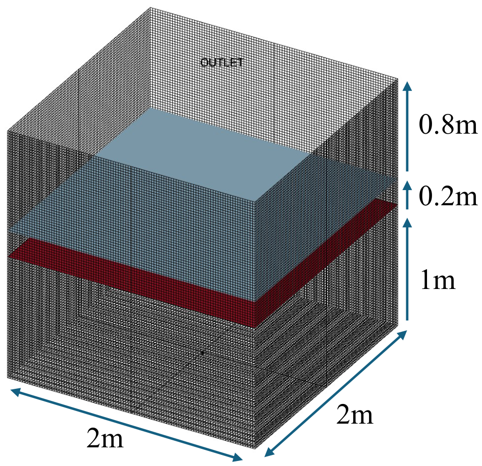
The bottom blow gas volume flow rate is . The inlet gas mass flow rate is
In Equation (112), , therefore .
The global initial temperature is
Equation (113) is used for the initial fields of molten steel, slag and gas phase; the subsequent energy source enters the energy equation through Equation (109) and is fed back to reaction balance, rate constants and reaction enthalpies through the bounded local-temperature treatment described above.
The initial three-layer phase distribution is
Equation (114) gives the phase-distribution initialisation used in this example. The calculation starts from a clear three-layer phase distribution, after which the mixed interface develops through Eulerian multifluid transport and interphase momentum exchange.
The numerical treatment first closes the reaction network and then limits the reacted amount in each time step by the local inventory. This preserves feedback among gas-phase oxygen supply, FeO oxygen supply, buffering, CaO dissolution, phosphate fixation and rephosphorisation, while avoiding the artificial conversion of local thermodynamic tendency into instantaneous global equilibrium.
2.10. Flow Controls and Solver Settings
The multiphase flow is solved with an Euler–Euler–DPM coupling scheme. The bottom-blown oxygen–lime-powder case is not a two-phase system with one clear free interface. It contains a bubble plume, molten metal, a continuous mixed-slag phase, locally generated FeO films and dissolving CaO particles. After oxygen enters the bath, iron oxide forms through gas–metal and gas–slag reactions. When CaO particles reach an effective slag region or an FeO-enriched reaction film, they dissolve and replenish the slag CaO inventory. These new slag regions and bubbles are spatially dispersed and often have low local volume fractions. A VOF calculation would have to resolve many low-volume-fraction slag droplets, bubble interfaces and newly generated slag regions on a limited grid. For the industrial bottom-blowing process considered here, such interface-by-interface resolution would greatly increase grid and time-step requirements and would make stable representation of phase volume fraction, reaction area and dispersed-phase volume source terms difficult. The Euler–Euler multifluid method is therefore used to describe molten steel, mixed slag and gas as interpenetrating continua, with phase volume fractions, phase velocities and phase-owned species as mean-field variables. DPM retains particle entry, migration, residence and dissolution. This combination avoids resolving each slag droplet and bubble while keeping oxygen supply, FeO generation, CaO entry into slag and slag–metal dephosphorisation in the same local conservation framework [23,24,25,26].
The current case is a three-dimensional, double-precision, unsteady multi-fluid calculation. A pressure-based finite-volume solver is used because molten steel, slag and gas remain in the low-Mach-number metallurgical-flow range; the dominant variables are phase volume fraction, pressure-velocity coupling, interphase momentum exchange, buoyancy and reaction source terms rather than compressible-wave propagation [99]. This choice is also consistent with the pressure-based multiphase implementation used for incompressible and weakly compressible Fluent calculations [101]. The calculation is advanced in time because particle residence, gas-plume growth, FeO accumulation, heat release and dephosphorisation sources are all history-dependent. Double precision is retained because small species such as , , and free-CaO enter the local reaction-window diagnosis.
Pressure-velocity coupling adopts the Phase Coupled SIMPLE scheme. SIMPLE-type pressure correction is the standard basis for segregated incompressible finite-volume flow solvers [99]. In a Euler–Euler bath with gas, slag and metal present simultaneously, the phase-coupled form corrects the shared pressure field and interphase momentum response together, which is more robust near the bottom plume where phase fraction, pressure gradient and slip velocity change rapidly [101]. The pressure, momentum and multiphase relaxation factors are set to 0.3, 0.7 and 0.5, respectively. The lower pressure relaxation suppresses oscillation from large density ratios and strong local volume sources, while the medium momentum and phase relaxation retain plume and slag-entrainment structures without making the transient update unstable.
The turbulence model adopts the k– SST model. The SST formulation blends near-wall k– behavior with far-field robustness and shear-stress transport, which is why it is commonly used for engineering flows involving wall shear, adverse pressure gradients and separation [102]. Its industrial use as a robust RANS closure for complex engineering CFD has also been documented in later SST experience studies [103]. Here it provides a reproducible mean mixing field for interphase area, particle residence and local source terms. LES and DES are not used because the target is furnace-scale reaction closure rather than resolving the full turbulent eddy spectrum. The k and equations use first-order upwind discretisation to improve robustness in strong-source multiphase regions.
The energy equation is enabled in all calculations and solved in conservative form. This treatment is used not only to obtain the temperature field, but also to let reaction heat affect thermodynamic equilibrium, phosphorus distribution, Arrhenius rates, oxygen potential and CaO-particle dissolution. The energy equation is discretised with the second-order upwind method, and the temperature relaxation factor is . Compared with momentum and phase volume fraction, the temperature field is controlled jointly by volumetric heat release and interphase transport. Second-order upwind discretisation reduces numerical smoothing of local hot spots, allowing reaction heat, gas-phase cooling and liquid-metal heat-capacity buffering near bottom-blown oxygen to retain clearer spatial gradients. Effective temperatures in thermodynamic and kinetic calculations are bounded above and below to prevent local numerical anomalies from driving equilibrium constants or rate constants outside their physical range.
The transient time step is taken as . This time step advances the continuous-phase flow field, phase volume fractions, energy equation and DPM particle trajectories together. The value is used because the bottom-blowing inlet velocity is high and the gas plume and CaO particles have short transport time scales near the inlet. If the time step is too large, particles may cross an effective reaction film or slag-capture region in one step, causing the CaO dissolution source and continuous-phase reaction source to become desynchronised. The current output corresponds to 40000 time steps, or of physical time. This interval is sufficient to observe early gas-channel formation, FeO enrichment, CaO entry into slag and the coupled response of decarburisation and dephosphorisation source terms.
The spatial discretisation is set hierarchically for stability and physical sensitivity. Body Force Weighted pressure interpolation is used because gravity, density difference and phase-volume-fraction gradients dominate the bath pressure field [101]. Momentum, phase volume fraction and turbulence transport are advanced with first-order upwind discretisation to prioritise boundedness near the inlet, gas–slag–metal mixing zone and strong source-term region. The energy equation uses second-order upwind discretisation to reduce numerical smoothing of local reaction-heating gradients, following the usual finite-volume tradeoff between bounded first-order convection and less diffusive higher-order transport [100].
Residual convergence criteria differ by equation type. Continuity, velocity, phase volume fraction, turbulence and component transport equations use , while the energy equation uses . The tighter energy residual is used because temperature directly enters equilibrium constants, phosphorus partitioning, reaction rates and reaction enthalpies. The residual criteria are combined with non-negativity, phase-existence and inventory limits so that iterative convergence and physical boundedness are checked together, consistent with source-term stabilisation practice in finite-volume multiphase CFD [99].
A supplementary VOF multiphase model is also provided for comparison. VOF is suitable for top-blown oxygen cases with clearer interfaces, but resolving the fine gas–slag–metal reaction interface in the present bottom-blown powder-injection case would require much higher grid and time-step resolution.
3. Results and Discussion
3.1. Phase Distribution and Effective Reaction Interface
Figure 2 defines the spatial setting for the reactions. The active region is not a static geometric slag–metal plane; it is a mixed zone produced by bubble plumes, slag entrainment, liquid-steel uplift, CaO-particle release and local interfacial area. The phase-volume-fraction scale of about – should be read as Eulerian phase occupation, not as a sharp interface. The interface-area-density fields convert this dispersed occupation into mean contact areas that can carry chemical source terms. This interpretation follows the continuum-averaged treatment of two-phase flow developed by Drew [23], is consistent with multicomponent-fluid theory [24], and follows standard Eulerian phase averaging in two-phase thermo-fluid modelling [25]. DPM is retained because powder trajectories and residence histories should not be collapsed into a uniform CaO source [32]. For dephosphorisation, the central step is to convert phase distribution into an effective reaction interface [91].
Under high-carbon conditions, the bottom plume follows the nozzle axis and expands in the slag–metal transition zone. The gas–metal interfacial area density reaches about , far above the gas–slag value of about and the slag–metal value of about . Endogenous CO from strong decarburisation therefore increases the gas inventory and renews gas–metal contact before it strengthens the slag–metal reaction. This is consistent with water-model studies linking bottom blowing to plume expansion and bath mixing [83] and with converter simulations showing the sensitivity of circulation to bottom-flow distribution [85]. A larger interface, however, does not automatically mean stronger dephosphorisation. The CaO source is concentrated near the bottom-blowing axis and the plume–slag contact region, with a local upper value of about . Powder-injection studies show that trajectory and residence time strongly affect the useful CaO fraction [38], and bottom-powder studies show that lance or tuyere structure changes the local utilisation path [39]. High-carbon stirring and local CaO supply contribute to dephosphorisation only when FeO retention and slag–metal contact occur in the same region.
In the low-carbon case, endogenous CO is weaker, the plume is narrower and more axially symmetric, and lateral entrainment is reduced. Less carbon is available to consume oxygen potential, so FeO and dissolved oxygen are more readily retained near the interface. The tradeoff is a more localised reaction space, which requires CaO release, FeO enrichment and slag–metal contact to overlap more precisely. This contrast gives the central mechanism: high carbon enhances mixing but consumes oxygen potential, whereas low carbon retains oxygen potential but weakens interface renewal. Furnace-scale equilibrium models can describe endpoint partitioning, but they cannot locate transient dephosphorisation sources in the bottom-blowing column [19]. Thermodynamic databases remain essential for slag capacity, but they must be coupled to local interface and inventory information to describe this non-uniform three-phase reaction [16].
3.2. Gas Reactions and Generation
Figure 3 shows that bottom-blown oxygen does not travel far through the bath as free . In both cases, is high only near the inlet and then falls rapidly. Away from the nozzle, the gas oxygen potential is controlled mainly by the buffer. In the high-carbon case, forms a broad high-value region near the central plume and slag–metal interface and locally approaches 0.95. The distribution shows that incoming is first converted to CO by the carbon–oxygen reaction; part of that CO is then oxidised to , and part rises with the bubbles. The coupled –– equilibrium in liquid iron provides the basis for this gas-buffer effect [50]. Iron-oxide reduction by carbon-bearing gas makes gas composition an active control variable for slag oxygen potential [95]. The activity relationship gives the corresponding slag-side redox response [51], and NIST thermochemical data provide the free-energy basis for the oxygen-potential calculation [48].
The height-wise partial-pressure and source-term curves separate this process further. From the inlet to about 0.35 m, is consumed rapidly and is co-generated. Between about 0.35 and 0.6 m, the gas composition shifts toward re-equilibration. Between 0.6 and 1.0 m, weak CO formation continues, while is still consumed or transformed. Near the upper slag layer, a small oxygen-potential exchange remains between and . The same zones appear in the low-carbon case, but the high-value gas regions are more concentrated. Carbon consumes less oxygen, so more oxygen potential can enter FeO generation and dissolved-oxygen channels. Early bottom-blown lime-oxygen experiments already showed that the dephosphorisation effect depends on local fluxing and slag formation rather than free oxygen alone [104]. Recent –CaO bottom-blowing work reaches the same process-level conclusion for high-efficiency dephosphorisation [36]. Lime-powder process studies also emphasize that local CaO–FeO liquid formation and mixing control the effective reaction window [105].
The gas phase therefore alternates among oxygen supply, decarburisation, buoyancy maintenance and redistribution. Under high-carbon conditions, gas generation strengthens the plume but shifts oxygen potential toward CO. Under low-carbon conditions, gas generation weakens, but oxygen potential is more readily retained at the slag–metal interface. This difference explains the later and distributions. Lime-powder dephosphorisation experiments similarly separate powder addition from the actual phosphorus-fixation step [106]. BOF off-gas studies also show that gas generation and post-combustion paths belong in the bath reaction balance [89].
3.3. Slag-Composition Evolution
Figure 4 shows how granular CaO is distributed after entering the continuous slag phase. The CaO increment enters along the bottom-blowing column and spreads laterally after the plume contacts the slag layer, so the DPM source is local rather than uniform. Part of the added CaO becomes liquid-CaO inventory, while free CaO is enriched near the plume edge at the slag–metal interface. This difference follows the local FeO distribution. When an FeO-rich liquid film is available, CaO can enter the liquid inventory more readily. When FeO near the plume edge is consumed by decarburisation, metal redox reactions and buffering, CaO is not fully absorbed and remains as free CaO. Solid-CaO reaction experiments show that CaO entry and useful dephosphorisation capacity are not the same event [43]. Lime dissolution studies identify FeO wetting and reaction-layer formation as the key controls on CaO availability [20]. Direct dissolution-rate measurements support the same dependence on slag composition and interfacial layer resistance [93].
FeO enrichment, CaO input and production are not synchronised. A CaO–iron-oxide reaction film appears in the bottom-blowing column, but is not generated continuously along that gas column. Its visible enrichment occurs mainly at the upper slag–metal interface, especially near the shoulder of the lifted interface. The – virtual phase contributes fixation capacity only where is actually generated. This agrees with solid-solution studies showing that – formation can lock phosphate in slag [13]. Interfacial-compound studies further show that local phase contact controls phosphate fixation rather than bulk CaO addition alone [66]. Recent slag studies likewise show that FeO content, alkalinity and solid-solution stability jointly determine whether phosphorus remains fixed [15]. The bottom-blowing column mainly supplies oxygen, slagging and mixing; the dephosphorisation window remains in the upper slag–metal mixing zone.
Figure 5 further traces this spatial difference to the dynamic transformation of . After bottom-blown oxygen enters, first establishes a FeO source near the injection axis. FeO can then decompose to release dissolved oxygen to the metal or be regenerated by . After the gas reaches the gas–slag and slag–metal mixing zone, Fe(II)/Fe(III) is controlled again by the balance, so can be reduced by CO or FeO can be reoxidised by . The net source is therefore not a single reaction rate, but a superposition of gas–metal oxygen supply, metal–slag oxygen exchange and gas–slag redox. Phosphate-capacity work shows that activity is central to high-basicity dephosphorisation slags [61]. BOF phosphorus-partition studies identify and basicity as coupled control variables [2]. Thermodynamic studies of activity explain why the same inventory can produce different phosphorus capacities under different slag compositions [56].
Under high-carbon conditions, is generated rapidly near the inlet but is reduced or redistributed by the CO-rich plume before it reaches the upper interface; a local negative source therefore appears at the interface edge. Under low-carbon conditions, carbon intercepts less oxygen potential, so the positive source extends more readily to the slag–metal interface. The decisive difference is not whether FeO is generated, but whether it remains near the effective interface after flotation, reduction and reoxidation. Phase-equilibrium work on CaO-containing slags shows that composition adjustment can improve thermodynamic dephosphorisation capacity [63], and calcium ferrite studies suggest another route for fluorite-free hot-metal dephosphorisation [82]. If is reduced in the reaction zone or consumed by decarburisation, however, those thermodynamic advantages do not translate into source-term strength. This explains why enrichment in Figure 4 is concentrated near the upper slag–metal interface.
3.4. Selectivity Among Decarburisation, Desiliconisation and Dephosphorisation
Figure 6 condenses the field variables into three reaction channels: decarburisation, desiliconisation and dephosphorisation. A necessary distinction is that represents an ideal phosphorus-partition capacity calculated from local slag composition, temperature and oxidation state; it is not the actual dephosphorisation rate. High may occur in the bottom-blowing column or in the slag layer, but it becomes real P removal only when available oxygen, a slag–metal interface, generation and – fixation coexist. Classical phosphorus-distribution relationships explain the endpoint partitioning trend [6]. BOF equilibrium-partition models provide a practical furnace-scale version of the same thermodynamic capacity [2]. They do not, by themselves, identify the transient location and source strength of dephosphorisation.
The source-term distribution shows that the bottom gas column is not the main dephosphorisation zone. It supplies oxygen, CaO and local FeO, but it does not provide stable – fixation. Liquid CaO represents alkalinity and CaO inventory, not final phosphorus fixation. The dephosphorisation source and – formation are concentrated near the upper slag–metal interface, where transfer, oxygen supply, generation and phosphate fixation can close in the same region. Kinetic experiments show that CaO–FeO–SiO2 dephosphorisation is controlled by coupled metal-side and slag-side mass transfer [41]. Oxidising-slag kinetics likewise show that increasing only one transport or slagging factor does not guarantee a proportional macroscopic P-removal rate [44]. Lime-dissolution measurements explain why the CaO source must be converted into usable slag capacity before it contributes to P fixation [93]. This is why appears at the upper interface in Figure 4 rather than continuously along the bottom-blowing column.
Reaction selectivity inside the bath is governed mainly by decarburisation. Bottom-blown oxygen first serves carbon removal. In the high-carbon case, the carbon channel persists along the injection axis and upper plume and is much stronger than the desiliconisation and dephosphorisation channels. Oxygen entering carbon-rich metal is preferentially consumed by to form CO, so local oxygen potential is not maintained long enough for stable and oxidation [50]. The reversible desiliconisation field also shows that the source term near the slag–metal interface does not keep the same sign everywhere. In CO-rich and -depleted regions, becomes less stable and local silicon return is thermodynamically allowed. Metal-droplet studies show that CO bubble generation can expand interfacial area while changing metal-side transport [46]. When the carbon reaction is too strong, intensified stirring mainly supports decarburisation rather than P fixation.
The high-carbon and low-carbon cases differ mainly in how they spend oxygen potential. The high-carbon bath has stronger stirring and larger interfacial area, but oxygen first enters decarburisation and CO buffering, and is reduced during flotation. In the low-carbon bath, decarburisation weakens and oxygen potential can enter and channels more easily, although interface renewal is less intense. The dephosphorisation ability of bottom-blown oxygen–CaO powder cannot be inferred from thermodynamic phosphorus capacity or stirring intensity alone. It depends on whether oxidation capacity, CaO supply, slag–metal contact and a fixation phase coexist. Continuous dephosphorisation practice uses staged refining to separate phosphorus removal from later decarburisation demand [75]. Double-slag operation follows the same logic by renewing slag capacity and controlling during converter refining [76]. Retained-slag and recycled-slag practices similarly use pre-existing slag capacity to improve hot-metal dephosphorisation [80].
3.5. Macroscopic Reaction Selectivity, Flow Sustainment and Thermal Feedback
Figure 7 connects the local source terms to macroscopic indicators. For element i, the element source term is integrated over the full computational domain and converted into the change rate of metal-phase mass fraction:
In Equation (115), is the local mass source term of element i, is the full computational domain, and and are the metal-phase density and volume fraction, respectively. The numerator is kg after full-field integration, and the denominator is the total metal-phase mass. The coefficient converts mass-fraction change per second into wt% . Thus, the column value in Figure 7(i) is a macroscopic removal rate and no longer has the dimension of the local volume source term.
The macroscopic integrals follow the local source-term pattern. In the high-carbon case, carbon is consumed mainly along the injection axis and upper plume, whereas phosphorus decreases only near the slag–metal interface. The integrated decarburisation rate is therefore much higher than the desiliconisation and dephosphorisation rates. In the low-carbon case, the decarburisation term contracts and the desiliconisation and dephosphorisation channels become visible in the integrated rates, but P consumption still does not extend through the whole bath. Lower carbon content releases oxygen potential, but it does not remove the need for an effective slag–metal interface and phosphate-fixation conditions. Endpoint P reduction is a whole-furnace integral result, not the direct contribution of one powder trajectory or one gas-column segment. Industrial –CaO bottom-blowing studies likewise report endpoint improvement only through coupled oxygen supply, slagging and bath mixing [36]. Double-slag studies show that slag amount and control remain decisive even when mixing is enhanced [77], and BOF dephosphorisation reviews identify slag composition and temperature as co-controlling variables [1].
The velocity and temperature fields show that reactions feed back into both flow and energy. Plume velocity does not decay rapidly after the gas leaves the inlet because CO generated by decarburisation continues to provide buoyancy in addition to the inlet momentum. This effect is stronger in the high-carbon case and weaker in the low-carbon case. In the energy field, the 300 K inlet gas first causes local cooling near the bottom; oxidation of Fe, C, Si and P and conversion then release reaction heat. Bottom-blowing water models have shown that plume buoyancy controls bath circulation [83], and converter simulations connect bottom-flow distribution with mixing intensity and plume persistence [85]. Gas–slag–metal emulsion simulations further show that the reaction zone is tied to the evolving plume rather than to a fixed geometric surface [87]. The present model extends that picture by treating gas generation as a source term that sustains buoyancy and interface renewal, not merely as a diagnostic output.
Reported hot-spot temperatures in oxygen steelmaking are often much higher than the temperature response in Figure 7(l), but the two quantities are not the same object. Literature values of 2000–C usually refer to the top-blown oxygen-jet impact cavity, where oxygen impinges directly on the metal surface and reaction heat is concentrated in a prescribed hot-spot zone [107,108]. Zone heat-balance and droplet heat-transfer models can also predict hot-spot temperatures of 1900–C, with peak values near C, because they treat the hot spot, slag/emulsion and hot-metal bath as coupled thermal zones and use prescribed reaction profiles or calibrated heat-transfer coefficients [109]. Those studies are useful references for top-blown BOF thermal behaviour, but they should not be used as a direct expectation for every cell near a bottom-blown oxygen nozzle.
The present calculation solves a moving, reaction-limited gas–slag–metal field rather than imposing a fixed hot-spot temperature. The plotted heat source is an instantaneous volumetric rate, not the cumulative heat retained in a stationary control volume. A local temperature increment scales with the retained residence time, , where is the volumetric heat-release rate, is the time over which the same material volume remains in the reactive region and represents heat carried away by convection, turbulent dispersion and interphase exchange. In the bottom plume, is short: liquid steel is swept upward, CO generation accelerates the plume, gas–metal slip renews the interface, and the 300 K injected gas introduces an initial cooling sink. Therefore, even when locally reaches the order of W , much of the released heat is transported with the flowing steel and dispersed into a larger bath volume before it can accumulate as a persistent superheated cell.
The thermal field is also limited chemically. Heat release is not calculated from a fixed stoichiometric oxygen-consumption rate at the tuyere; it is constrained by local availability, carbon competition, conversion, slag–metal contact and CaO-assisted reaction capacity. Regions with strong decarburisation generate CO and buoyancy, but they do not necessarily retain high oxygen potential or high long enough to sustain both heat release and dephosphorisation. Thus, the modest temperature rise in Figure 7(l) is consistent with a convective, reaction-limited bottom-blowing process. Thermal feedback mainly changes gas generation, interphase slip and interface renewal near the plume rather than producing the persistent high-temperature impact spot expected from fixed-zone top-blowing calculations. Under the present conditions, P removal is limited primarily by the spatial coincidence of oxygen potential, slag–metal interface and phosphate-fixation capacity, not by the absence of reaction heat.
3.6. Overall Reaction Mechanism
Figure 8 places the particle-scale interpretation from the literature and the field-resolved result from the present calculation in the same framework. Wang Chunyang’s schematic for a bottom-blown ––lime-powder process emphasises that CaO particles may undergo CaO–FeO liquid-film fluxing, CaO–SiO2 shell formation during flotation, CaO–P2 reaction and – fixation [110]. Bottom-blown lime-oxygen studies support the view that CaO particles can react rapidly once they encounter an FeO-rich liquid film [34]. Lime-powder dephosphorisation tests show that the final contribution still depends on particle residence path and coupling with the slag–metal interface [111]. Observing phosphorus-containing calcium silicate or – products near particles therefore does not by itself prove that a macroscopic dephosphorisation channel has been established.
Macroscopic dephosphorisation requires five processes to close continuously within the same effective slag–metal contact zone: transfer to the interface, oxygen supply, CaO-particle dissolution, generation and – fixation. That closure is difficult to sustain under high-carbon conditions. Bottom-blown oxygen first enters the decarburisation channel, and the resulting lowers retention during flotation. Even when P oxidation occurs locally, or when a – transition product forms, the product may redissolve and rephosphorise in a later reducing region. Observing – in an experiment therefore does not by itself prove stable dephosphorisation capacity in the high-carbon stage. It may instead record a transient local state of oxygen potential and CaO activity. This interpretation can accommodate two apparently conflicting observations: a phosphorus-enriched phase may form near particles, while the macroscopic decrease of P in the metal remains limited or is dominated by top-slag reactions and later low-carbon stages.
This point matters for experimental attribution. In bottom-blown ––lime-powder or oxygen–lime-powder experiments, endpoint P can decrease because of top-slag reaction, a higher furnace oxygen potential, changes in slag volume and basicity, improved mixing or a changed temperature schedule. It should not be assigned automatically to direct dephosphorisation during powder flotation. The calculations here support that distinction. Bottom powder first improves local slag formation, CaO transport and plume mixing. A stable dephosphorisation window opens only when carbon–oxygen competition weakens and the CaO–FeO liquid film, liquid-CaO/free-CaO inventory, retention and upper slag–metal interface overlap. For hot metal or the early high-carbon converter stage, the direct dephosphorisation contribution of bottom-blown oxygen–lime powder is limited, and the strong plume may even suppress net P removal by consuming oxygen potential and promoting interfacial re-reduction. The process is better understood as a route for enhanced slagging and local low-carbon-stage dephosphorisation, or as part of a double-slag, retained-slag or pretreatment strategy. If the bottom gas column is expected to carry the main dephosphorisation burden in high-carbon hot metal, the powder-flotation contribution is likely to be overestimated.
4. Conclusions
This study establishes an Euler–Euler–DPM framework for gas–slag–metal–particle reactions in steelmaking and applies it to bottom-blown oxygen–CaO-powder dephosphorisation. The framework does not reduce dephosphorisation to a single empirical source term. It places gas-phase oxygen potential, valence conversion, CaO-particle dissolution, slag–metal interfacial reaction, generation, – fixation and reaction-heat feedback in one conservative system. It therefore addresses a question that conventional thermodynamic models cannot answer directly: where do oxygen, CaO, and P meet in a non-uniform bottom-blown bath, and where can they form a sustainable dephosphorisation window?
The effective reaction zone is neither the static slag–metal plane nor the bottom gas column alone. It is a local mixing zone formed by bubble plumes, slag entrainment, liquid-steel uplift, CaO input to slag and mean-field interfacial area. Under high-carbon conditions, CO generated by strong decarburisation expands the gas–metal interface and strengthens plume disturbance. Under low-carbon conditions, the plume is narrower and interface renewal is weaker, but oxygen potential is more likely to be retained at the slag–metal interface. Stirring intensity and dephosphorisation capacity therefore do not have a simple monotonic relation. A strong plume becomes useful for P removal only when oxygen potential, CaO and a fixation phase are present together.
The main selectivity constraint is carbon. In a high-carbon bath, bottom-blown oxygen serves decarburisation before it serves dephosphorisation. is rapidly consumed near the inlet, and gas-phase oxygen potential is then buffered through . CO generation sustains plume buoyancy and renews interfaces, but it also weakens retention during flotation. The high-carbon case therefore has stronger flow and more interface, yet less oxidation capacity remains available to stabilise oxidised P and fix .
CaO particles do not automatically capture phosphorus after entering the bath. Once particles enter the effective slag phase or a CaO–FeO liquid reaction film, part of their mass becomes liquid-CaO inventory and part remains as free CaO near the edge of the FeO-depleted plume. CaO input can improve local slag formation and basicity, but it becomes dephosphorisation capacity only when oxygen supply, generation and – fixation close within the same slag–metal contact zone. The calculations show that generation and – fixation occur mainly at the upper slag–metal interface, not inside the bottom-blowing column.
The phosphorus partitioning ratio cannot be read as the actual dephosphorisation rate. A local slag phase can have a high ideal , but if oxygen potential is intercepted by carbon reaction, or if stable slag–metal contact and phosphate fixation are absent, the high represents only thermodynamic capacity. It does not mean that P has been removed. Under high-carbon conditions, even locally formed or – transition products may redissolve and rephosphorise in later CO-rich and -depleted regions. A microscopic phosphorus-containing phase is therefore not equivalent to a macroscopically stable dephosphorisation channel.
In process terms, bottom-blown oxygen–CaO powder is better viewed as a means of enhanced slagging and local low-carbon-stage dephosphorisation, not as the primary dephosphorisation mechanism during early high-carbon hot-metal or converter blowing. Under low-carbon conditions, carbon–oxygen competition weakens, is more readily retained, and CaO–FeO liquid, liquid-CaO/free-CaO inventory and the upper slag–metal interface are more likely to overlap. The dephosphorisation window then opens. In the high-carbon bath, bottom powder mainly promotes local slagging, mixing and plume restructuring. Without support from top slag, retained slag, double-slag practice or a later low-carbon stage, its direct dephosphorisation contribution is strongly suppressed by decarburisation.
Overall, the model is neither a flow calculation with chemistry added afterwards nor an endpoint-equilibrium dephosphorisation model. It is a closed description in which flow creates interface, interface carries reaction, and reaction feeds back into flow and temperature. The practical requirement for industrial dephosphorisation is not simply more oxygen, more CaO or stronger stirring. oxygen supply, effective CaO dissolution, slag–metal interface renewal and phosphate fixation must occur together at the right time and in the right region. This framework provides a scalable basis for analysing bottom-powder injection, combined-blown converters, low-carbon endpoint dephosphorisation and related gas–slag–metal reaction processes.
Data Availability Statement
The code and case files are available at https://github.com/Zhenkeaidai/DeC-Si-P-in-Steel-Maker-CFD-work.git
Acknowledgments
All authors have read and agreed to the published version of the manuscript. This was financially supported by the National Natural Science Foundation of China (grant No. 52304430 by H.Wang).
Conflicts of Interest
The authors declare no conflicts of interest.
References
- Lin, W.; Jiao, S.; Zhou, K.; Sun, J.; Feng, X.; Liu, Q. A Review of Multi-phase Slag Refining for Dephosphorization in the Steelmaking Process. Front. Mater. 2020, 7. [Google Scholar] [CrossRef]
- Drain, P.B.; Monaghan, B.J.; Zhang, G.; Longbottom, R.J.; Chapman, M.W.; Chew, S.J. A review of phosphorus partition relations for use in basic oxygen steelmaking. Ironmak. Steelmak. 2017, 44, 721–731. [Google Scholar] [CrossRef]
- Wang, Z.L.; Song, T.L.; Zhao, L.H.; Bao, Y.P. Study on Efficient Dephosphorization in Converter Based on Thermodynamic Calculation. Crystals 2023, 13, 1132. [Google Scholar] [CrossRef]
- Keskinkilic, E. New trends in basic oxygen furnace dephosphorization. J. Min. Metall. Sect. B Metall. 2020, 56, 1–10. [Google Scholar] [CrossRef]
- Li, Z.; Li, J.; Spooner, S.; Seetharaman, S. Basic Oxygen Steelmaking Slag: Formation, Reaction, and Energy and Material Recovery. Steel Res. Int. 2021, 93. [Google Scholar] [CrossRef]
- SUITO, H.; INOUE, R.; TAKADA, M. Phosphorus distribution between liquid iron and MgO saturated slags of the system CaO-MgO-FeOx-SiO2. Trans. Iron Steel Inst. Jpn. 1981, 21, 250–259. [Google Scholar] [CrossRef]
- SUITO, H.; INOUE, R. Effect of Calcium Fluoride on Phosphorus Distribution between MgO Saturated Slags of the System CaO-MgO-FeOx-SiO2 and Liquid Iron. Trans. Iron Steel Inst. Jpn. 1982, 22, 869–877. [Google Scholar] [CrossRef]
- SUITO, H.; INOUE, R. Phosphorus distribution between MgO-saturated CaO-FetO-SiO2-P2O5-MnO slags and liquid iron. Trans. Iron Steel Inst. Jpn. 1984, 24, 40–46. [Google Scholar] [CrossRef]
- Basu, S.; Lahiri, A.K.; Seetharaman, S. Phosphorus Partition between Liquid Steel and CaO-SiO2-P2O5-MgO Slag Containing Low FeO. Metall. Mater. Trans. B 2007, 38, 357–366. [Google Scholar] [CrossRef]
- Inoue, R.; Suito, H. Phosphorous Partition between 2CaO SiO2 Particles and CaO-SiO2-FetO Slags. ISIJ Int. 2006, 46, 174–179. [Google Scholar] [CrossRef]
- Suito, H.; Inoue, R. Behavior of Phosphorous Transfer from CaO-FetO-P2O5(-SiO2) Slag to CaO Particles. ISIJ Int. 2006, 46, 180–187. [Google Scholar] [CrossRef]
- Shimauchi, K.i.; Kitamura, S.y.; Shibata, H. Distribution of P2O5 between Solid Dicalcium Silicate and Liquid Phases in CaO–SiO2–Fe2O3 System. ISIJ Int. 2009, 49, 505–511. [Google Scholar] [CrossRef]
- Kitamura, S.y.; Saito, S.; Utagawa, K.; Shibata, H.; Robertson, D.G.C. Mass Transfer of P2O5 between Liquid Slag and Solid Solution of 2CaO·SiO2 and 3CaO·P2O5. ISIJ Int. 2009, 49, 1838–1844. [Google Scholar] [CrossRef]
- Zhu, B.; Zhu, M.; Luo, J.; Dou, X.; Wang, Y.; Jiang, H.; Xie, B. Distribution Behavior of Phosphorus in 2CaO·SiO2-3CaO·P2O5 Solid Solution Phase and Liquid Slag Phase. Metals 2020, 10, 1103. [Google Scholar] [CrossRef]
- Song, Y.; Hu, X.; Chou, K. The Reaction Behavior of 2CaO·SiO2 with CaO–SiO2–FeO–P2O5 Slag. Materials 2022, 15, 6594. [Google Scholar] [CrossRef] [PubMed]
- Jung, I.H.; Hudon, P.; Kim, W.Y.; van Ende, M.A.; Rahman, M.; Curiel, G.G. Thermodynamic Database of P 2 O 5 -containing Oxide Systems for the Dephosphorization Process in Steelmaking. htmp 2013, 32, 247–254. [Google Scholar] [CrossRef]
- Bale, C.; Chartrand, P.; Degterov, S.; Eriksson, G.; Hack, K.; Ben Mahfoud, R.; Melançon, J.; Pelton, A.; Petersen, S. FactSage thermochemical software and databases. Calphad 2002, 26, 189–228. [Google Scholar] [CrossRef]
- Bale, C.; Bélisle, E.; Chartrand, P.; Decterov, S.; Eriksson, G.; Gheribi, A.; Hack, K.; Jung, I.H.; Kang, Y.B.; Melançon, J.; et al. FactSage thermochemical software and databases, 2010–2016. Calphad 2016, 54, 35–53. [Google Scholar] [CrossRef]
- Mason, P.; Grundy, A.N.; Rettig, R.; Kjellqvist, L.; Jeppsson, J.; Bratberg, J. The Application of an Effective Equilibrium Reaction Zone Model Based on CALPHAD Thermodynamics to Steel Making. In The Minerals, Metals & Materials Series 11th International Symposium on High-Temperature Metallurgical Processing; Springer International Publishing, 2020; pp. 101–113. [Google Scholar] [CrossRef]
- Hamano, T.; Fukagai, S.; Tsukihashi, F. Reaction Mechanism between Solid CaO and FeOx–CaO–SiO2–P2O5 Slag at 1 573 K. ISIJ Int. 2006, 46, 490–495. [Google Scholar] [CrossRef]
- Xie, S.; Wang, W.; Liu, Y.; Matsuura, H. Effect of Na2O and B2O3 on the Distribution of P2O5 between Solid Solution and Liquid Phases Slag. ISIJ Int. 2014, 54, 766–773. [Google Scholar] [CrossRef]
- Li, J.y.; Zhang, M.; Guo, M.; Yang, X.m. Phosphate enrichment mechanism in CaO–SiO2–FeO–Fe2O3–P2O5 steelmaking slags with lower binary basicity. Int. J. Miner. Metall. Mater. 2016, 23, 520–533. [Google Scholar] [CrossRef]
- Drew, D.A. Mathematical Modeling of Two-Phase Flow. Annu. Rev. Fluid Mech. 1983, 15, 261–291. [Google Scholar] [CrossRef]
- Drew, D.A.; Passman, S.L. Theory of Multicomponent Fluids; Applied Mathematical Sciences; Springer New York, 1999. [Google Scholar] [CrossRef]
- Ishii, M.; Hibiki, T. Thermo-Fluid Dynamics of Two-Phase Flow; Springer New York, 2011. [Google Scholar] [CrossRef]
- Besagni, G.; Varallo, N.; Mereu, R. CFD Modelling of Two-Phase Bubble Columns: A Comprehensive Review. Fluids 2023, 8, 91. [Google Scholar] [CrossRef]
- Lv, M.; Chen, S.; Yang, L.; Wei, G. Research Progress on Injection Technology in Converter Steelmaking Process. Metals 2022, 12, 1918. [Google Scholar] [CrossRef]
- Cappel, J.; Ahrenhold, F.; Egger, M.W.; Hiebler, H.; Schenk, J. 70 Years of LD-Steelmaking–Quo Vadis? Metals 2022, 12, 912. [Google Scholar] [CrossRef]
- Zhou, C.; Li, J.; Yuan, T.; Yan, Z.; Gong, W.; Ai, L.; Wang, S.; Gao, X. Study on the Mechanism of CaO–SiO2–FeO–P2O5 Dephosphorization Slag Under Different FeO Contents and Basicity. Steel Res. Int. 2024, 96. [Google Scholar] [CrossRef]
- Coetsee, T.; De Bruin, F. EERZ (Effective Equilibrium Reaction Zone) Model of Gas-Slag-Metal Reactions in the Application of Unconstrained Al-Ni-Cr-Co-Cu Metal Powders in Submerged Arc Welding: Model and 3D Slag SEM Evidence. Processes 2023, 11, 2110. [Google Scholar] [CrossRef]
- Ekambara, K.; Nandakumar, K.; Joshi, J.B. CFD Simulation of Bubble Column Reactor Using Population Balance. Ind. Eng. Chem. Res. 2008, 47, 8505–8516. [Google Scholar] [CrossRef]
- van Sint Annaland, M.; Deen, N.; Kuipers, J. Numerical simulation of gas–liquid–solid flows using a combined front tracking and discrete particle method. Chem. Eng. Sci. 2005, 60, 6188–6198. [Google Scholar] [CrossRef]
- Gualtieri, C.; Angeloudis, A.; Bombardelli, F.; Jha, S.; Stoesser, T. On the Values for the Turbulent Schmidt Number in Environmental Flows. Fluids 2017, 2, 17. [Google Scholar] [CrossRef]
- HAIDA, O.; TAKEUCHI, S.; NOZAKI, T.; EMI, T.; SUDO, F. Mechanism of Hot Metal Dephosphorization by Injecting Lime Base Fluxes into Bottom Blown Converter. Tetsu-to-Hagane 1982, 68, 1744–1753. [Google Scholar] [CrossRef] [PubMed]
- ONO, H.; MASUI, T.; MORI, H. Dephosphorization Kinetics of Hot Metal by Lime Injection with Oxygen Gas. Tetsu-to-Hagane 1983, 69, 1763–1770. [Google Scholar] [CrossRef] [PubMed]
- Li, W.; Zhu, R.; Dong, K.; Zhang, J.; Feng, C.; Han, B.; Wu, X. Physical Simulation and Industrial Testing of Bottom-Blown O2-CaO Converter for Steelmaking Process. Metall. Mater. Trans. B 2020, 51, 1060–1069. [Google Scholar] [CrossRef]
- Zhang, K.; Wang, S.; Li, C.; Yuan, Z.; Zhang, Y. Numerical simulation of multiphase flow induced by bottom blowing limestone powder in converter steelmaking. Powder Technol. 2025, 449, 120369. [Google Scholar] [CrossRef]
- Hu, S.; Zhu, R.; Wang, D.; Li, X.; Wei, G. Research on the Gas–Solid Jet Flow and Erosion Wear Characteristics in Bottom Injecting Lance Used for Oxygen–Lime Powder Bottom Blowing Converter. Metall. Mater. Trans. B 2021, 52, 3875–3887. [Google Scholar] [CrossRef]
- Zhang, J.; Lou, W.; Zhu, M. Numerical Simulation of Particle Motion and Wall Scouring Behavior in Steelmaking Converter With Bottom Powder Injection. Metall. Mater. Trans. B 2023, 54, 3031–3048. [Google Scholar] [CrossRef]
- Tang, B.; Wang, X.; Zou, Z.; Yu, A. Physical simulation of converter steelmaking with powder injection. Can. Metall. Q. 2016, 55, 124–130. [Google Scholar] [CrossRef]
- KAWAI, Y.; DOI, S.; MORI, K. Rate of Dephosphorization of Liquid Iron by CaO-FeO-SiO2 Slag. Tetsu-to-Hagane 1977, 63, 391–399. [Google Scholar] [CrossRef] [PubMed]
- KUNISADA, K.; IWAI, H. Rate of Dephosphorization of Liquid Iron by the Slag of CaO-SiO2-FeO System. Tetsu-to-Hagane 1984, 70, 1681–1688. [Google Scholar] [CrossRef] [PubMed]
- ARATANI, F.; SANBONGI, K. Kinetic Study of Dephosphorization of Liquid Iron with Solid CaO. Tetsu-to-Hagane 1972, 58, 1217–1224. [Google Scholar] [CrossRef] [PubMed]
- Monaghan, B.J.; Pomfret, R.J.; Coley, K.S. The kinetics of dephosphorization of carbon-saturated iron using an oxidizing slag. Metall. Mater. Trans. B 1998, 29, 111–118. [Google Scholar] [CrossRef]
- Gu, K.; Dogan, N.; Coley, K.S. The Influence of Sulfur on Dephosphorization Kinetics Between Bloated Metal Droplets and Slag Containing FeO. Metall. Mater. Trans. B 2017, 48, 2343–2353. [Google Scholar] [CrossRef]
- Gu, K.; Dogan, N.; Coley, K.S. Dephosphorization Kinetics between Bloated Metal Droplets and Slag Containing FeO: The Influence of CO Bubbles on the Mass Transfer of Phosphorus in the Metal. Metall. Mater. Trans. B 2017, 48, 2984–3001. [Google Scholar] [CrossRef]
- Kitamura, S.y.; Miyamoto, K.i.; Shibata, H.; Maruoka, N.; Matsuo, M. Analysis of Dephosphorization Reaction Using a Simulation Model of Hot Metal Dephosphorization by Multiphase Slag. ISIJ Int. 2009, 49, 1333–1339. [Google Scholar] [CrossRef]
- Linstrom, P.J.; Mallard, W.G. NIST Chemistry WebBook. NIST Stand. Ref. Database Number 2026, 69. [Google Scholar] [CrossRef]
- Sigworth, G.K.; Elliott, J.F. The Thermodynamics of Liquid Dilute Iron Alloys. Metal. Sci. 1974, 8, 298–310. [Google Scholar] [CrossRef]
- El-Kaddah, N.H.; Robertson, D.G.C. Equilibria in reactions of CO and CO2 with dissolved oxygen and carbon in liquid iron. Metall. Trans. B 1977, 8, 569–579. [Google Scholar] [CrossRef]
- Henao, H.M.; Itagaki, K. Activity and Activity Coefficient of Iron Oxides in the Liquid FeO-Fe2O3-CaO-SiO2 Slag Systems at Intermediate Oxygen Partial Pressures. Metall. Mater. Trans. B 2007, 38, 769–780. [Google Scholar] [CrossRef]
- Basu, S.; Lahiri, A.K.; Seetharaman, S. Phosphorus Partition between Liquid Steel and CaO-SiO2-FeO x -P2O5-MgO Slag Containing 15 to 25 Pct FeO. Metall. Mater. Trans. B 2007, 38, 623–630. [Google Scholar] [CrossRef]
- Choudhary, S.K.; Lenka, S.N.; Ghosh, A. Assessment and application of equilibrium slag–metal phosphorous partition for basic oxygen steelmaking. Ironmak. Steelmak. 2007, 34, 343–349. [Google Scholar] [CrossRef]
- Assis, A.N.; Tayeb, M.A.; Sridhar, S.; Fruehan, R.J. Phosphorus Equilibrium Between Liquid Iron and CaO-SiO2-MgO-Al2O3-FeO-P2O5 Slag Part 1: Literature Review, Methodology, and BOF Slags. Metall. Mater. Trans. B 2015, 46, 2255–2263. [Google Scholar] [CrossRef]
- N. Assis, A.; A. Tayeb, M.; Sridhar, S.; J. Fruehan, R. Phosphorus Equilibrium Between Liquid Iron and CaO-SiO2-MgO-Al2O3-FeO-P2O5 Slags: EAF Slags, the Effect of Alumina and New Correlation. Metals 2019, 9, 116. [Google Scholar] [CrossRef]
- Turkdogan, E.T. Assessment of P2O5 Activity Coefficients in Molten Slags. ISIJ Int. 2000, 40, 964–970. [Google Scholar] [CrossRef]
- Lee, C.M.; Fruehan, R.J. Phosphorus equilibrium between hot metal and slag. Ironmak. Steelmak. 2005, 32, 503–508. [Google Scholar] [CrossRef]
- Kovtun, O.; Karbayev, M.; Korobeinikov, I.; Srishilan, C.; Shukla, A.K.; Volkova, O. Phosphorus Partition Between Liquid Crude Steel and High-Basicity Basic Oxygen Furnace Slags. Steel Res. Int. 2021, 92. [Google Scholar] [CrossRef]
- Neubert, L.; Kovtun, O.; Kreschel, T.; Volkova, O. Phosphorus Partition Between Liquid Crude Steel and High-Basicity Basic Oxygen Furnace Slags Containing V2O5. Metall. Mater. Trans. B 2023, 54, 1524–1531. [Google Scholar] [CrossRef]
- Kim, S.J.; Takekawa, J.; Shibata, H.; Kitamura, S.y.; Yamaguchi, K.; Kang, Y.B. Thermodynamic Assessment of MnO and FeO Activities in FeO–MnO–MgO–P2O5–SiO2(–CaO) Molten Slag. ISIJ Int. 2013, 53, 1325–1333. [Google Scholar] [CrossRef]
- SHIROTA, Y.; KATOHGI, K.; KLEIN, K.; ENGELL, H.J.; JANKE, D. Phosphate capacity of FeO-Fe2O3-CaO-P2O5 and FeO-Fe2O3-CaO-CaF2-P2O5 slags by levitation melting. Trans. Iron Steel Inst. Jpn. 1985, 25, 1132–1140. [Google Scholar] [CrossRef]
- Watanabe, K.; Miki, T.; Sasaki, Y.; Hino, M. Phase Relation of CaO-Al2O3-FetO-P2O5 Slag and Phosphorus Distribution between This Slag and Liquid Iron. Tetsu-to-Hagane 2009, 95, 217–221. [Google Scholar] [CrossRef]
- Gao, X.; Matsuura, H.; Miyata, M.; Tsukihashi, F. Phase Equilibrium for the CaO–SiO2–FeO–5mass%P2O5–5mass%Al2O3 System for Dephosphorization of Hot Metal Pretreatment. ISIJ Int. 2013, 53, 1381–1385. [Google Scholar] [CrossRef]
- Geng, B.; Zhan, D.; Jiang, Z.; Yang, Y. Effect of CaO-MgO-FeO-SiO2-xNa2O Slag System on Converter Dephosphorization. Metals 2023, 13, 844. [Google Scholar] [CrossRef]
- Kami, M.; Terasawa, M.; Matsumoto, A.; Ito, K. The Model Experiment on the Formation of 2CaO SiO2-3CaO P2O5 Phase in the Dephosphorization Slag. Tetsu-to-Hagane 2009, 95, 236–240. [Google Scholar] [CrossRef]
- Yang, X.; Matsuura, H.; Tsukihashi, F. Formation Behavior of Phosphorous Compounds at the Interface between Solid 2CaO SiO2 and FeOx-CaO-SiO2-P2O5 Slag at 1673K. Tetsu-to-Hagane 2009, 95, 268–274. [Google Scholar] [CrossRef]
- Yang, X.; Matsuura, H.; Tsukihashi, F. Condensation of P2O5 at the Interface between 2CaO·SiO2 and CaO–SiO2–FeOx–P2O5 Slag. ISIJ Int. 2009, 49, 1298–1307. [Google Scholar] [CrossRef]
- Li, J.y.; Zhang, M.; Guo, M.; Yang, X.M. Enrichment Mechanism of Phosphate in CaO-SiO2-FeO-Fe2O3-P2O5 Steelmaking Slags. Metall. Mater. Trans. B 2014, 45, 1666–1682. [Google Scholar] [CrossRef]
- Du, C.m.; Gao, X.; Ueda, S.; Kitamura, S.y. Distribution of P2O5 and Na2O Between Solid Solution and Liquid Phase in the CaO-SiO2-Fe2O3-P2O5-Na2O Slag System with High P2O5 Content. Metall. Mater. Trans. B 2017, 49, 181–189. [Google Scholar] [CrossRef]
- Du, C.m.; Lv, N.n.; Su, C.; Liu, W.m.; Yang, J.x.; Wang, H.c. Distribution of P2O5 between solid solution and liquid phase in dephosphorization slag of CaO–SiO2–FeO–P2O5–Na2O system. J. Iron Steel Res. Int. 2019, 26, 1162–1170. [Google Scholar] [CrossRef]
- Li, C.; Gao, J.; Guo, Z. Separation of Phosphorus- and Iron-Enriched Phase from CaO-SiO2-FeO-MgO-P2O5 Melt with Super Gravity. Metall. Mater. Trans. B 2016, 47, 1516–1519. [Google Scholar] [CrossRef]
- Meija, J.; Coplen, T.B.; Berglund, M.; Brand, W.A.; De Bièvre, P.; Gröning, M.; Holden, N.E.; Irrgeher, J.; Loss, R.D.; Walczyk, T.; et al. Atomic weights of the elements 2013 (IUPAC Technical Report). Pure Appl. Chem. 2016, 88, 265–291. [Google Scholar] [CrossRef]
- Tiesinga, E.; Mohr, P.J.; Newell, D.B.; Taylor, B.N. CODATA Recommended Values of the Fundamental Physical Constants: 2018. J. Phys. Chem. Ref. Data 2021, 50. [Google Scholar] [CrossRef] [PubMed]
- YOSHIDA, K.; YAMAZAKI, I.; TOZAKI, Y.; AOKI, N.; YOSHIYAMA, J.i.; ARAI, K. Development of Effective Refining Process Consisting of both Hot Metal Pretreatment and Decarburization in Two Top and Bottom Blown Converters. Tetsu-to-Hagane 1990, 76, 1817–1822. [Google Scholar] [CrossRef] [PubMed]
- OGAWA, Y.; YANO, M.; KITAMURA, S.; HIRATA, H. Development of the Continuous Dephosphorization and Decarburization Process Using BOF. Tetsu-to-Hagane 2001, 87, 21–28. [Google Scholar] [CrossRef] [PubMed]
- Wu, W.; Dai, S.f.; Liu, Y. Dephosphorization stability of hot metal by double slag operation in basic oxygen furnace. J. Iron Steel Res. Int. 2017, 24, 908–915. [Google Scholar] [CrossRef]
- Sun, H.; Yang, J.; Lu, X.; Liu, W.; Ye, G.; Zhang, R.; Yang, W. Dephosphorization in Double Slag Converter Steelmaking Process at Different Temperatures by Industrial Experiments. Metals 2021, 11, 1030. [Google Scholar] [CrossRef]
- Kang, Y. Desiliconisation and Dephosphorisation Behaviours of Various Oxygen Sources in Hot Metal Pre-Treatment. Metals 2019, 9, 251. [Google Scholar] [CrossRef]
- Volkova, O.; Tinkova, N.; Onaa, R.I.; Neubert, L.; Niziaiev, K.; Zotov, D. Phosphorus Partition in an Industrial Basic Oxygen Furnace Process in Ukraine. Steel Res. Int. 2024, 96. [Google Scholar] [CrossRef]
- Bai, X.f.; Sun, Y.h.; Luo, L.; Zhao, C.l. Effect of direct charging of hot recycled slag on hot metal pretreatment dephosphorization in a dephosphorization furnace. J. Iron Steel Res. Int. 2019, 27, 148–159. [Google Scholar] [CrossRef]
- Diao, J.; Xie, B.; Wang, Y.; Guo, X. Recovery of Phosphorus from Dephosphorization Slag Produced by Duplex High Phosphorus Hot Metal Refining. ISIJ Int. 2012, 52, 955–959. [Google Scholar] [CrossRef]
- Wu, W.; Zhao, B.; Zhao, B.; Wu, W.; Meng, H.d. Hot metal dephosphorization process using calcium ferrite slag without fluorite. Ironmak. Steelmak. 2022, 49, 661–668. [Google Scholar] [CrossRef]
- Ballal, N.B.; Ghosh, A. A water model study of bottom-blown oxygen steelmaking processes. Metall. Trans. B 1981, 12, 525–534. [Google Scholar] [CrossRef]
- Li, Y.; Lou, W.T.; Zhu, M.Y. Numerical simulation of gas and liquid flow in steelmaking converter with top and bottom combined blowing. Ironmak. Steelmak. 2013, 40, 505–514. [Google Scholar] [CrossRef]
- Chu, K.Y.; Chen, H.H.; Lai, P.H.; Wu, H.C.; Liu, Y.C.; Lin, C.C.; Lu, M.J. The Effects of Bottom Blowing Gas Flow Rate Distribution During the Steelmaking Converter Process on Mixing Efficiency. Metall. Mater. Trans. B 2016, 47, 948–962. [Google Scholar] [CrossRef]
- Li, M.; Li, Q.; Zou, Z.; Li, B. Characterization of Cavity Oscillation and Splashing Distribution Under Excitation by Bottom Gas Blowing in a Steelmaking Converter. JOM 2018, 71, 729–736. [Google Scholar] [CrossRef]
- Lv, M.; Li, H.; Lin, T.; Xie, K.; Xue, K. Behavior of Gas–Slag–Metal Emulsion with Nozzle-Twisted Lance in Converter Steelmaking Process. Steel Res. Int. 2021, 92. [Google Scholar] [CrossRef]
- Dong, P.; Zheng, S.; Zhu, M. Numerical Study on Gas-Metal-Slag Interaction with Single-Flow Postcombustion Oxygen Lance in the Steelmaking Process of a Top-Blown Converter. JOM 2022, 74, 1509–1520. [Google Scholar] [CrossRef]
- Li, S.; Wei, X.; Yu, L. Numerical simulation of off-gas formation during top-blown oxygen converter steelmaking. Fuel 2011, 90, 1350–1360. [Google Scholar] [CrossRef]
- Luomala, M.J.; Fabritius, T.M.J.; Virtanen, E.O.; Siivola, T.P.; Härkki, J.J. Splashing and Spitting Behaviour in the Combined Blown Steelmaking Converter. ISIJ Int. 2002, 42, 944–949. [Google Scholar] [CrossRef]
- Cai, X.; Duan, H.; Xu, A.; Chen, W.; Zhang, L. Mathematical Modeling on the Multiphase Flow during Top–Bottom Combined Blowing Basic Oxygen Furnace Steelmaking Process. Steel Res. Int. 2024, 96. [Google Scholar] [CrossRef]
- Hamano, T.; Horibe, M.; Ito, K. The Dissolution Rate of Solid Lime into Molten Slag Used for Hot-metal Dephosphorization. ISIJ Int. 2004, 44, 263–267. [Google Scholar] [CrossRef]
- Kikuchi, N.; Matsui, A.; Uchida, Y.i. Effect of Lime Dissolution Rate in Slag on Hot Metal Dephosphorization. ISIJ Int. 2020, 60, 922–929. [Google Scholar] [CrossRef]
- Ishikawa, M. Reduction Behaviors of Hot Metal Dephosphorization Slag in a Slag Regenerator. ISIJ Int. 2006, 46, 530–538. [Google Scholar] [CrossRef]
- Paul, A.; Deo, B.; Sathyamurthy, N. Kinetic model for reduction of iron oxide in molten slags by iron-carbon melt. Steel Res. 1994, 65, 414–420. [Google Scholar] [CrossRef]
- Maxey, M.R.; Riley, J.J. Equation of motion for a small rigid sphere in a nonuniform flow. Phys. Fluids 1983, 26, 883–889. [Google Scholar] [CrossRef]
- Tenneti, S.; Subramaniam, S. Particle-Resolved Direct Numerical Simulation for Gas-Solid Flow Model Development. Annu. Rev. Fluid Mech. 2014, 46, 199–230. [Google Scholar] [CrossRef]
- Zhou, Z.; Pinson, D.; Zou, R.; Yu, A. Discrete particle simulation of gas fluidization of ellipsoidal particles. Chem. Eng. Sci. 2011, 66, 6128–6145. [Google Scholar] [CrossRef]
- Patankar, S.V. Numerical Heat Transfer and Fluid Flow; Hemisphere Publishing Corporation: Washington, DC, 1980. [Google Scholar]
- Versteeg, H.K.; Malalasekera, W. An Introduction to Computational Fluid Dynamics: The Finite Volume Method, 2 ed.; Pearson Education: Harlow, 2007. [Google Scholar]
- ANSYS Inc. ANSYS Fluent Theory Guide, 2025. Release 2025 R1.
- Menter, F.R. Two-Equation Eddy-Viscosity Turbulence Models for Engineering Applications. AIAA J. 1994, 32, 1598–1605. [Google Scholar] [CrossRef] [PubMed]
- Menter, F.R.; Kuntz, M.; Langtry, R. Ten Years of Industrial Experience with the SST Turbulence Model. In Turbulence, Heat and Mass Transfer 4; Begell House, 2003; pp. 625–632. [Google Scholar]
- Nozaki, T.; Takeuchi, S.; Haida, O.; Emi, T.; Morishita, H.; Sudo, F. Mechanism of hot metal dephosphorization by injecting lime base fluxes with oxygen into bottom blown converter. Trans. Iron Steel Inst. Jpn. 1983, 23, 513–521. [Google Scholar] [CrossRef]
- Wang, C.; Dong, K.; Xue, Z.; Zhao, C.; Guan, S.; Ding, G.; Feng, C.; Zhu, R. High-Efficiency Dephosphorization by Bottom-Blown O2-CaO Process for Semi-Steelmaking. Steel Res. Int. 2024, 95, 2300457. [Google Scholar] [CrossRef]
- Miyata, M.; Tamura, T.; Higuchi, Y. Development of Hot Metal Dephosphorization with Lime Powder Top Blowing: Part 1. Low Blowing Rate. ISIJ Int. 2017, 57, 1751–1755. [Google Scholar] [CrossRef]
- Singha, P.; Shukla, A.K. Contribution of Hot-Spot Zone in Decarburization of BOF Steel-Making: Fundamental Analysis Based upon the FactSage-Macro Program. Metals 2022, 12, 638. [Google Scholar] [CrossRef]
- Mitas, B.; Schenk, J. Oxygen Distribution at the Hot Spot in BOF Steelmaking. Metall. Mater. Trans. B 2024, 55, 1680–1689. [Google Scholar] [CrossRef]
- Madhavan, N.; Brooks, G.A.; Rhamdhani, M.A.; Rout, B.K.; Overbosch, A. Global Droplet Heat Transfer in Oxygen Steelmaking Process. Metals 2022, 12, 992. [Google Scholar] [CrossRef]
- Wang, C. Mechanism of Dephosphorization in Converter Bottom-Blown O2-CO2-Lime Powder Process. PhD thesis, in Chinese. University of Science and Technology Beijing, 2025. [Google Scholar]
- Miyata, M.; Tamura, T.; Higuchi, Y. Development of Hot Metal Dephosphorization with Lime Powder Top Blowing: Part 2. High Blowing Rate. ISIJ Int. 2017, 57, 1756–1761. [Google Scholar] [CrossRef]
Figure 2.
Three-phase distribution, particle-to-slag source term and mean-field reaction interfaces for the high-carbon and low-carbon cases. The upper row (a–i) is the high-carbon case with initial composition , and ; the lower row (j–r) is the low-carbon case with initial composition , and . Steel, Slag and Gas denote the volume fractions of the liquid steel, slag and gas phases. DPM denotes the volumetric source by which CaO particles release material into the slag phase. Gas–Slag Interface, Metal–Slag Interface and Gas–Metal Interface denote the corresponding mean-field interfacial area densities. Gas Iso-Sur. and Slag Iso-Sur. show high-volume-fraction isosurfaces of the gas and slag phases.
Figure 2.
Three-phase distribution, particle-to-slag source term and mean-field reaction interfaces for the high-carbon and low-carbon cases. The upper row (a–i) is the high-carbon case with initial composition , and ; the lower row (j–r) is the low-carbon case with initial composition , and . Steel, Slag and Gas denote the volume fractions of the liquid steel, slag and gas phases. DPM denotes the volumetric source by which CaO particles release material into the slag phase. Gas–Slag Interface, Metal–Slag Interface and Gas–Metal Interface denote the corresponding mean-field interfacial area densities. Gas Iso-Sur. and Slag Iso-Sur. show high-volume-fraction isosurfaces of the gas and slag phases.
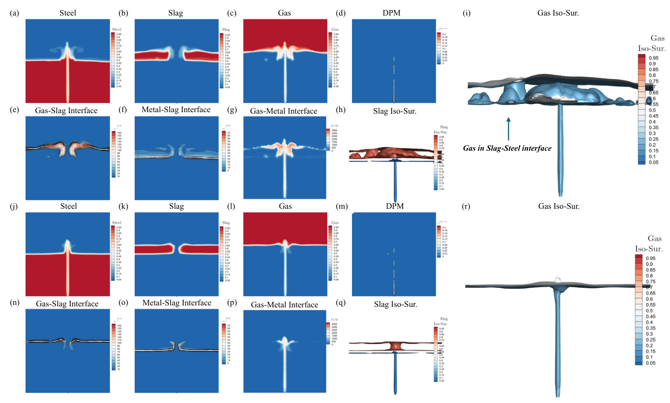
Figure 3.
Gas partial pressures, gas-reaction source terms and axial evolution in the high-carbon and low-carbon cases. The upper row (a–f) is the high-carbon case and the lower row (g–l) is the low-carbon case. Panels (a–c,g–i) show the spatial distributions of , and , respectively. Panels (d–f,j–l) show the source terms associated with , and , where positive values indicate generation and negative values indicate consumption. Panels (m) and (n) give height-wise profiles of gas partial pressures and gas source terms.
Figure 3.
Gas partial pressures, gas-reaction source terms and axial evolution in the high-carbon and low-carbon cases. The upper row (a–f) is the high-carbon case and the lower row (g–l) is the low-carbon case. Panels (a–c,g–i) show the spatial distributions of , and , respectively. Panels (d–f,j–l) show the source terms associated with , and , where positive values indicate generation and negative values indicate consumption. Panels (m) and (n) give height-wise profiles of gas partial pressures and gas source terms.
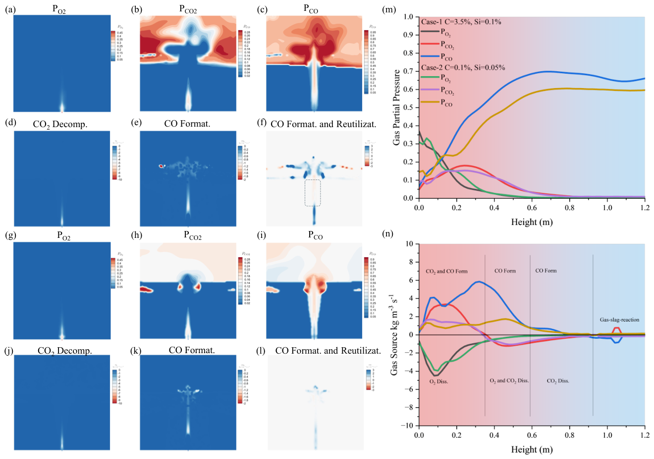
Figure 4.
Slag-composition evolution in the high-carbon and low-carbon cases. The upper panels correspond to the high-carbon case and the lower panels to the low-carbon case. CaO Increase denotes the incremental source by which CaO enters the continuous slag phase from particles. Liquid-CaO Mass Frac. and Free-CaO Mass Frac. denote the liquid CaO inventory and the free-CaO mass fraction. FeO Mass Frac. and Mass Frac. denote the slag iron-oxide components. C2SC3P Mass Frac. denotes the virtual – fixation phase, and Mass Frac. denotes the mass fraction in the slag.
Figure 4.
Slag-composition evolution in the high-carbon and low-carbon cases. The upper panels correspond to the high-carbon case and the lower panels to the low-carbon case. CaO Increase denotes the incremental source by which CaO enters the continuous slag phase from particles. Liquid-CaO Mass Frac. and Free-CaO Mass Frac. denote the liquid CaO inventory and the free-CaO mass fraction. FeO Mass Frac. and Mass Frac. denote the slag iron-oxide components. C2SC3P Mass Frac. denotes the virtual – fixation phase, and Mass Frac. denotes the mass fraction in the slag.
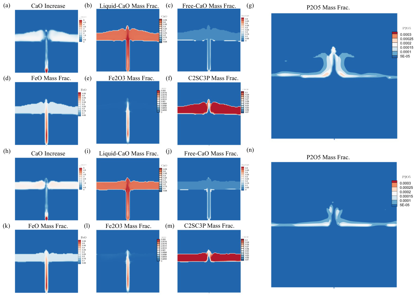
Figure 5.
Slag iron-oxide reaction channels and total source terms in the high-carbon and low-carbon cases. The upper panels correspond to the high-carbon case and the lower panels to the low-carbon case. Panels (a,h) show , (b,i) show , (c,j) show , (d,k) show , and (e,l) show . Panels (f,m) show total distribution and (g,n) show the net source term.
Figure 5.
Slag iron-oxide reaction channels and total source terms in the high-carbon and low-carbon cases. The upper panels correspond to the high-carbon case and the lower panels to the low-carbon case. Panels (a,h) show , (b,i) show , (c,j) show , (d,k) show , and (e,l) show . Panels (f,m) show total distribution and (g,n) show the net source term.
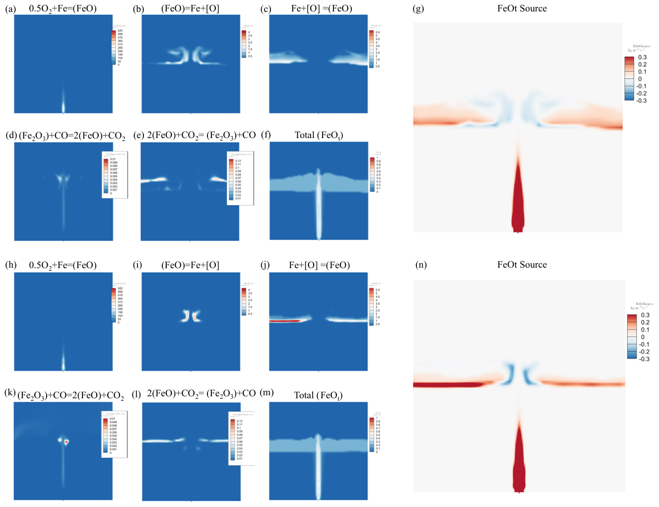
Figure 6.
Spatial distributions and representative profiles of phosphorus partitioning, dephosphorisation, – fixation, desiliconisation and decarburisation in the high-carbon and low-carbon cases. The upper row (a–e) is the high-carbon case and the lower row (f–j) is the low-carbon case. Panels (a,f) show calculated from local slag composition, (b,g) show the dephosphorisation source term, (c,h) show the formation source of the virtual – fixation phase, (d,i) show the desiliconisation/resiliconisation source term and (e,j) show the decarburisation source term. Panels (k–m) give path profiles along the bottom-blowing axis, the mid-height transverse section and the upper slag–metal interface.
Figure 6.
Spatial distributions and representative profiles of phosphorus partitioning, dephosphorisation, – fixation, desiliconisation and decarburisation in the high-carbon and low-carbon cases. The upper row (a–e) is the high-carbon case and the lower row (f–j) is the low-carbon case. Panels (a,f) show calculated from local slag composition, (b,g) show the dephosphorisation source term, (c,h) show the formation source of the virtual – fixation phase, (d,i) show the desiliconisation/resiliconisation source term and (e,j) show the decarburisation source term. Panels (k–m) give path profiles along the bottom-blowing axis, the mid-height transverse section and the upper slag–metal interface.
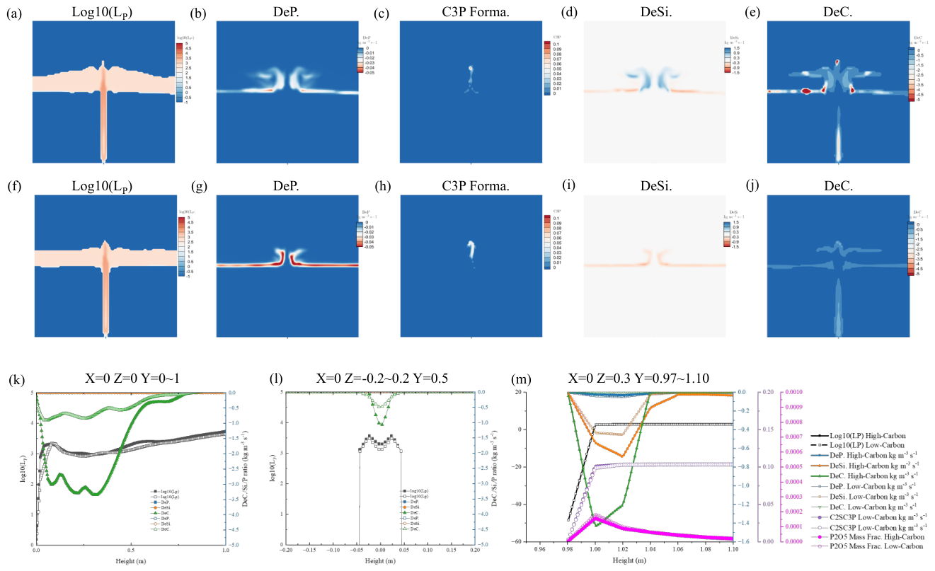
Figure 7.
Macroscopic composition fields, velocity fields and thermal feedback in the high-carbon and low-carbon cases. The upper row (a–d) is the high-carbon case and the lower row (e–h) is the low-carbon case. Panels (a,e) show the C mass fraction in liquid steel, (b,f) show the P mass fraction in liquid steel, (c,g) show velocity magnitude and (d,h) show the volumetric energy source. Panel (i) shows macroscopic decarburisation, desiliconisation and dephosphorisation rates obtained by integrating source terms over the whole domain, in wt% . Panels (j–l) give axial velocity, reaction heat source and temperature distributions.
Figure 7.
Macroscopic composition fields, velocity fields and thermal feedback in the high-carbon and low-carbon cases. The upper row (a–d) is the high-carbon case and the lower row (e–h) is the low-carbon case. Panels (a,e) show the C mass fraction in liquid steel, (b,f) show the P mass fraction in liquid steel, (c,g) show velocity magnitude and (d,h) show the volumetric energy source. Panel (i) shows macroscopic decarburisation, desiliconisation and dephosphorisation rates obtained by integrating source terms over the whole domain, in wt% . Panels (j–l) give axial velocity, reaction heat source and temperature distributions.
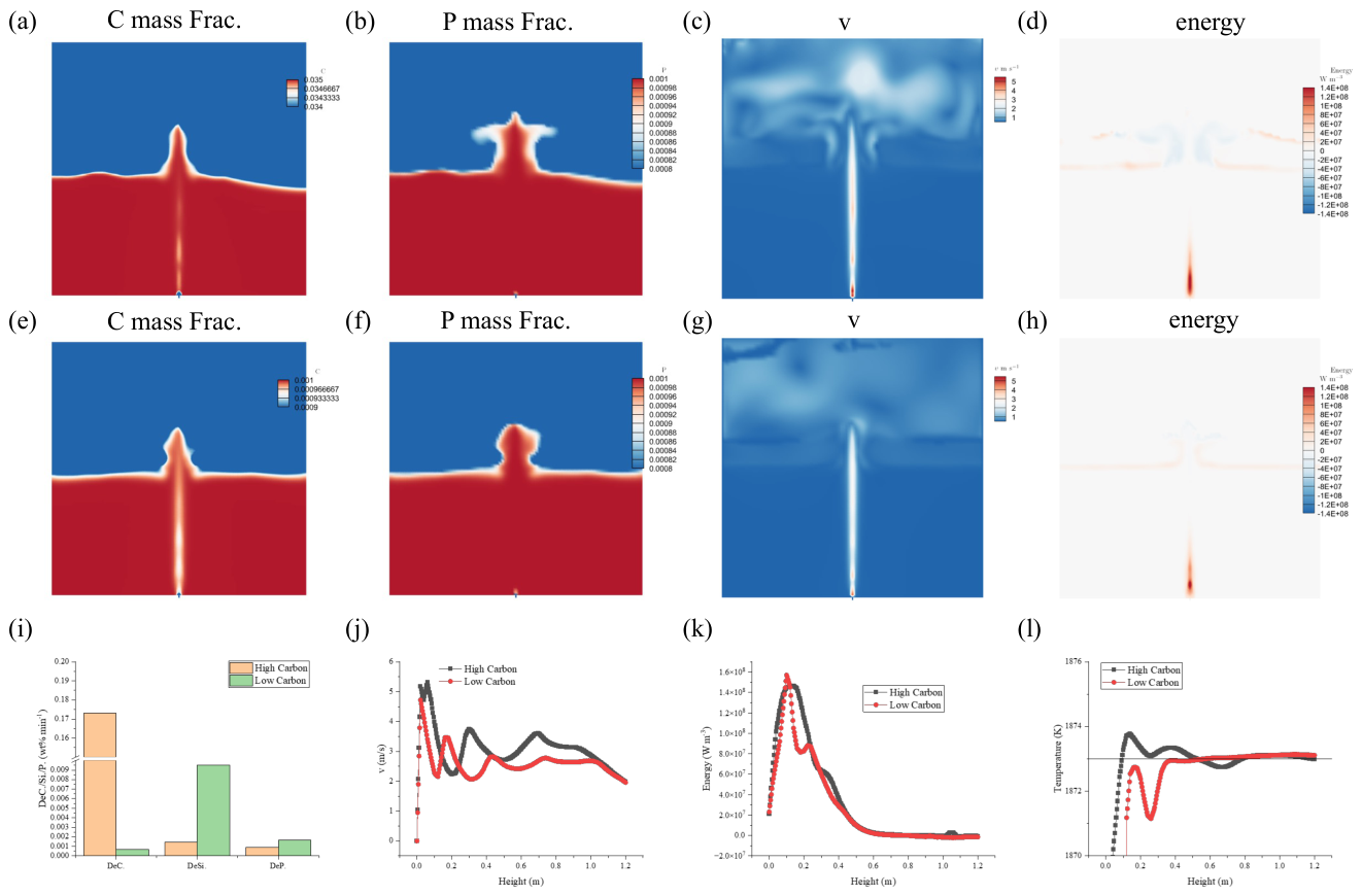
Figure 8.
Schematic mechanism of gas–slag–metal coupled dephosphorisation in the bottom-blown oxygen–CaO powder system. Panel (a) is redrawn from Wang Chunyang’s schematic of CaO-particle floating and reaction behaviour in a bottom-blown ––lime-powder process[110] (redrawn). Panel (b) shows the field-resolved mechanism inferred from the present calculations.
Figure 8.
Schematic mechanism of gas–slag–metal coupled dephosphorisation in the bottom-blown oxygen–CaO powder system. Panel (a) is redrawn from Wang Chunyang’s schematic of CaO-particle floating and reaction behaviour in a bottom-blown ––lime-powder process[110] (redrawn). Panel (b) shows the field-resolved mechanism inferred from the present calculations.
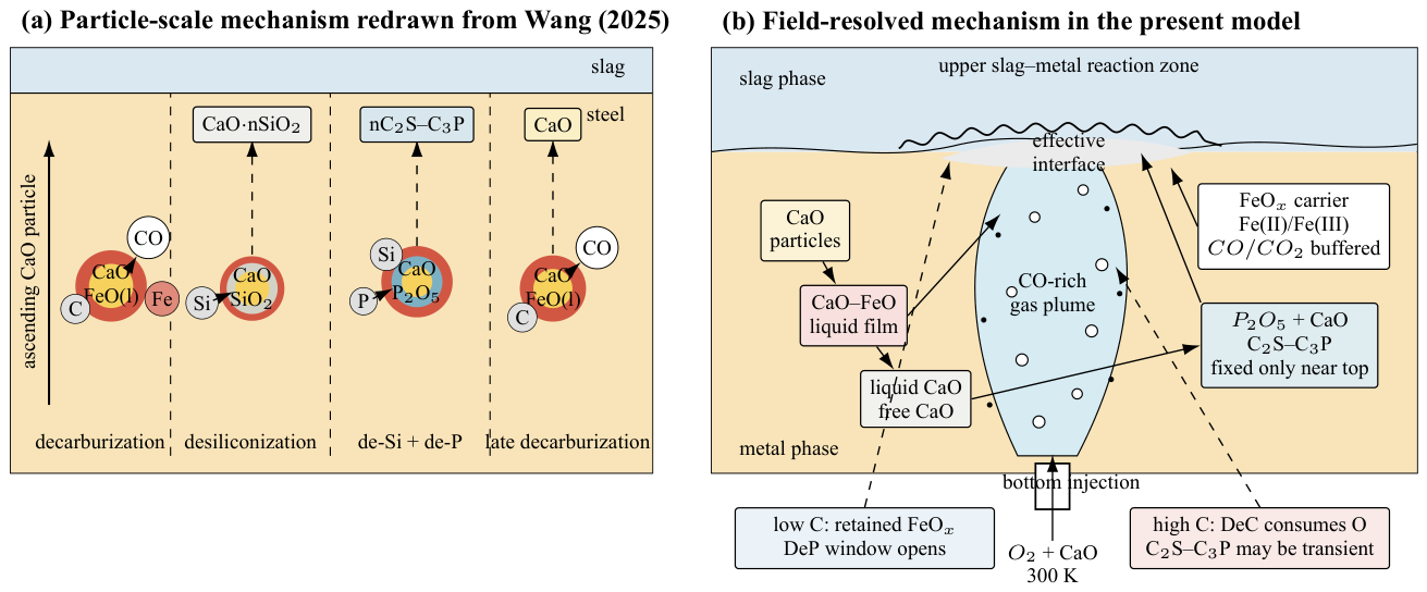
Table 1.
Reaction rates, closure reactions and the corresponding changes in the gas, slag and metal compositions.
Table 1.
Reaction rates, closure reactions and the corresponding changes in the gas, slag and metal compositions.
| rate | closure reaction | Gas phase changes | Metal phase changes | Slag phase changes | effect |
|---|---|---|---|---|---|
| is consumed as a balance metal | FeO is generated at the gas–metal contact, and the product is included in the slag oxide inventory. | ||||
| no direct changes | Metal dissolved oxygen continues to generate FeO at the metal–slag interface. | ||||
| no direct changes | The inlet oxygen directly enters the metal dissolved oxygen reservoir. | ||||
| no direct changes | FeO in the slag supplies oxygen to the metal when it is deficient in oxygen. | ||||
| no direct changes | no direct changes | The CO produced by decarburisation continues to consume oxygen and increase the partial pressure. | |||
| no direct changes | cracks for oxygen and CO–[O] recombination closes at the same signed rate. | ||||
| no direct changes | The decarburisation reaction connects metallic carbon to gas phase CO. | ||||
| no direct changes | Silicon oxidation preferentially consumes dissolved oxygen and increases acidic oxides. | ||||
| no direct changes | Direct oxidative dephosphorisation channel. | ||||
| no direct changes | Forward metal-to-slag phosphorus transfer driven by partition disequilibrium. | ||||
| no direct changes | Limited rephosphorisation channel under conditions of high phosphate or low oxygen potential. | ||||
| no direct changes | Gas–slag oxygen transfer raises the ferric-iron fraction in the slag. | ||||
| no direct changes | oxidises FeO to higher-valence iron while generating CO. | ||||
| no direct changes | CO from decarburisation reduces ferric iron and closes the indirect post-combustion loop. | ||||
| no direct changes | no direct changes | The internal phase distribution of CaO particles after dissolution does not produce a new fluid phase. | |||
| no direct changes | no direct changes | A dicalcium silicate skeleton is generated. | |||
| no direct changes | no direct changes | Fixes and increases the end-member share in the solid phase. | |||
| no direct changes | no direct changes | The first-order weight loss source of particles in the effective slag phase or FeO reaction film is split into two parts: CaO directly entering the liquid slag and temporary free-CaO. |
Table 3.
Final case settings and their physical purpose.
| case | Initial molten steel mass fraction | initial dissolved oxygen | Set purpose |
|---|---|---|---|
| Case H | , , | High carbon, low silicon, phosphorus-containing benchmark conditions. This setting retains strong decarburisation, CO generation, CO afterburning and oxygen potential buffering, so that the model simultaneously faces the competition of oxygen consumption by carbon, FeO generation, CaO dissolution and phosphorus migration. It is the most stringent case to test the closure of the three-phase reaction. | |
| Case L | , , | Low carbon, low silicon, same as initial phosphorus conditions. This setting weakens the buffering effect of decarburisation on the oxygen potential, so that dephosphorisation is mainly controlled by oxygen supply, oxidation and reduction, effective dissolution of CaO and slag–metal-phosphorus distribution. It is used to evaluate the competition between continued dephosphorisation and potential rephosphorisation in the liquid steel near the end. |
Disclaimer/Publisher’s Note: The statements, opinions and data contained in all publications are solely those of the individual author(s) and contributor(s) and not of MDPI and/or the editor(s). MDPI and/or the editor(s) disclaim responsibility for any injury to people or property resulting from any ideas, methods, instructions or products referred to in the content. |
© 2026 by the authors. Licensee MDPI, Basel, Switzerland. This article is an open access article distributed under the terms and conditions of the Creative Commons Attribution (CC BY) license (http://creativecommons.org/licenses/by/4.0/).
Copyright: This open access article is published under a Creative Commons CC BY 4.0 license, which permit the free download, distribution, and reuse, provided that the author and preprint are cited in any reuse.