

Submitted:
14 July 2026
Posted:
15 July 2026
You are already at the latest version
Abstract
Ionospheric response to a geomagnetic storm depends on several factors. Strength of a storm, commencement type, type of the solar origin of a geomagnetic storm (e.g., coronal mass ejections or high-speed solar wind streams) and observational site location are among them. In this work we present the results of a statistical analysis of eighty moderate to major geomagnetic storms that took place during the declining phase of the 24th solar cycle, from 2015 to 2019. We carried out an analysis on the ionospheric response to these storms using the total electron content (TEC) data obtained from three geodetic receivers located in Portugal: Lisbon (Continental Portugal), Furnas (Azores) and Funchal (Madeira). Two of the receivers, at Lisbon and Azores, are located at about the same latitude (~39ºN) while the third receiver, at Madeira, is positioned to the south (~33ºN). The receivers are also distributed in longitude from 9ºW to 25ºW. Statistical analysis of the observed TEC variations allowed detection of specific patterns in the ionospheric response to storms with different characteristics. Special attention was given to the longitudinal and latitudinal (dis)similarities in the ionospheric variations, observed at the three studied locations.
Keywords:
ionosphere at middle latitudes
; geomagnetic storms
; total electron content
1. Introduction
Empirical models are one of the most actively developed types of the ionospheric models. They are based on observational data and statistical analysis of such data to relate observed variations of, e.g., the total electron content (TEC) with such external forcings as solar flares, geomagnetic storms, and other space weather events [1,2]. These models are developed both on different spatial scales, from the global down to the regional or even single location models. Recent advance in the neural network (NN) development resulted in an explosive growth of new ionospheric models which provide, as a rule, better forecasting quality comparing to the classical empirical models based on, e.g., statistical, regression or correlation analyses [see [1,2] and references therein].
The forecasting quality of the empirical models is not uniform. They provide low error forecasts for quiet periods—periods without solar flares or geomagnetic storms, but the (geomagnetic) storm-time forecasting is still a significant challenge [1,2,3].
Geomagnetic storms (GM storms) are an important space weather phenomenon that, apart from affecting ground and satellite based technological and high frequency communications systems, can severely affect the dynamics and structure of the Earth’s entire thermosphere and ionosphere. Ionospheric response to a geomagnetic storm is called an ionospheric storm or disturbance (here we use a term “ionospheric disturbance” to distinguish it from “geomagnetic storm”) and describes the variations of the ionospheric conditions only due to geomagnetic events. Ionospheric variations can be determined from TEC, from the critical frequency of an ionospheric layer (e.g., f0F2 for the F2 layer), or from the peak electron density of an ionospheric layer (e.g., NmF2 for the F2 layer). These parameters show specific variations, an increase or decrease, relative to their average quiet time levels, which are known as positive or negative, respectively, ionospheric storms [4,5]. The type (positive or negative) of the ionospheric response to a GM storm depends on many conditions. These conditions include the strength of a geomagnetic storm, the local time of its commencement, a season, a solar activity level that affects the type of the GM storm solar source, latitude and longitude of a location of interest.
Unfortunately, few studies have been performed on a long-term analysis of the ionospheric disturbances caused by GM storms: most of the studies one can find are focused on a small number of outstanding geomagnetic events and cannot be used to deduce statistical patterns of an ionospheric response to a GM storm. Besides, as is shown both in the long-term studies and in the individual case analyses, the ionospheric response to a storm is not spatially uniform: it varies across the latitudes and the longitudes. The latter is not only due to the different local time at different longitudinal zones, but also is caused by the regional peculiarities, e.g., due to the geomagnetic equator position or regional atmospheric features [6]. Among the long-term studies of the ionospheric storm-time behaviour we would like to highlight the works of [7,8,9,10]. The first two present the analysis of the events observed in the Euro-African longitudinal sector, and the last two are focused on the American sector. In general, there is a strong similarity in the results obtained for the middle and low latitudes (which are the focus area for our study) in different longitudinal sectors, however some differences can be found even inside the same longitudinal zone [9].
To summarise the results of [7,8,9,10], the ionospheric response to a GM storm at the middle-to-low latitudes is, most often, a positive one, especially for GM storms that started during the daytime hours, while for the storms commenced during the night hours negative ionospheric disturbances or delayed (to the next day) positive disturbances are observed more frequently. Another important parameter of a GM storm that affects the ionospheric response is the type of the GM storm commencement (SC): gradual or sudden (GSC or SSC, respectively). GSC geomagnetic storms tend to produce a delayed ionospheric response more often, while for the SSC storms which trigger a negative ionospheric disturbance, the amplitude of the ionospheric parameters variations is higher than for other events [7,8]. Also, it was shown, both by [7,8] and [10], that more negative ionospheric disturbances are observed at lower latitudes compared to the mid-latitudinal regions. Some of the features of storm-time ionospheric response are the same for all longitudinal sectors, others significantly change [10,11].
Thus, the development of a good empirical regional ionospheric model requires a thorough preliminary study of the regional ionospheric response to geomagnetic storms of different kinds (commencement time and type, season, origin, etc.). While NN and other machine learning techniques are good at picking up specific patterns by themselves (in comparison to, e.g., regression models [2,3]), the forecasting quality of such models during the GM storm time is still insufficient. The incorporation of pre-found relations between certain characteristics of a GM storm and ionospheric response at a certain region or location seems to be a logical step in the development of the next generation of empirical models for the ionospheric storm-time variations.
The goal of this study is to identify such relations or most prominent patterns in the response of the regional ionosphere to GM storms. The study is focused on the statistical analysis of the storms-time ionospheric response in the middle-to-low latitudes (30º-40º N) of the eastern North Atlantic region (25º-0º E). A previously performed case study of the ionospheric disturbances associated with several intense-to-major geomagnetic storms of the last decade showed notable differences in the ionospheric response between locations at 40º N and 30ºN (Lisbon and Azores islands, and Madeira, respectively) [12]. This difference was confirmed by modelling the ionosphere at those locations [2]: the models were trained on the local ionospheric data (TEC) and a set of space weather parameters that includes geomagnetic indices and parameters of the solar wind. The forecasting quality of the models developed for Madeira was slightly lower than for more northern locations (Lisbon and Azores), suggesting an existence of other forcings not accounted for by the models (presumably, a coupling with the low-latitudinal and equatorial ionosphere). To examine further the similarity and differences in the longitudinal and latitudinal response of the ionosphere to geomagnetic storms we performed a long-term statistical analysis studying a wide range of geomagnetic storms observed during the last 5 years of the 24th solar cycle (2015–2019). In this paper we present the results of the statistical analysis of such characteristics of TEC variations at Lisbon, Azores and Madeira as their type, length and the amplitude, in relation to the solar (solar activity level, solar sources of geomagnetic storms) and geomagnetic (strength of GM storms, their commencement type) conditions.
2. Data
2.1. Total Electron Content Data
The ionospheric TEC data used in this work covers the time interval between January 2015 and December 2019, corresponding to the decreasing phase of the 24th solar cycle. The TEC data were collected at three Portuguese locations: Lisbon (Cascais) at the Continental Portugal, either Furnas or Ponta Delgada at S. Miguel Island of the Azores archipelago (see Table 1 for detail) and Funchal at Madeira. The locations and other details are shown in Table 1 and Figure 1.
The TEC data are derived from the GNSS (Global Navigation Satellite System) RINEX (Receiver Independent Exchange Format) files. Two data sources were used:
- The data from January to June 2015 and from January 2017 to December 2019 are from GNSS receivers of the national network of geodetic receivers RENEP (Rede Nacional de Estações Permanentes GNSS, https://renep.dgterritorio.gov.pt/ (accessed on 30 June 2026).
- The data gap (from July 2015 to December 2016) in the RENEP data was filled up with the data from the EUREF Permanent GNSS Network (EPN, https://www.epncb.oma.be/_networkdata/data_access/, accessed on 30 June 2026).
RENEP provides data in the RINEX 2.11 format. These files were processed and calibrated using the GNSS Lab (http://www.gnss-lab.org/ (accessed on 30 June 2026) and TEQC (https://www.unavco.org/software/data-processing/teqc/teqc.html (accessed on 30 June 2026, see the website for the updated information about the manufacturer and currently available versions) software as described in [12]. EUREF provides data in the Compact RINEX format. These files were processed and calibrated using the GPS-TEC software by G. Seemala (https://seemala.blogspot.com/, accessed on 30 June 2026) [13].
The TEC data are in TEC units (1 TECu = 1016 electrons/m2). All the TEC series used in this work have 1h time resolution.
2.2. Geomagnetic and Solar Data
The geomagnetic storms were identified and characterized using the Dst and Kp geomagnetic indices obtained from the Kyoto World Data Centre (WDC) and from GFZ Helmholtz Centre, Potsdam, Germany, respectively. Only moderate to major geomagnetic storms were studied. The storms were classified by the minimum Dst values observed during the storm: moderate GM storms with -100 nT ≤Dstmin ≤ -50 nT, intense storms with -200 nT ≤Dstmin ≤ -100 nT and major storms with Dstmin ≤ -200 nT.
The main sources of geomagnetic storms are coronal mass ejections (CMEs) and corotating interaction regions producing corotating streams or high-speed solar streams (HSS). CMEs are believed to be the primary cause of the largest and most damaging space weather events. The occurrence rate of CMEs increases during the maximum of the solar activity cycle. HSS are, mostly, generated in coronal holes and may interact with the slow solar wind. They become more frequent during the declining phase of a solar cycle [14]. When a strong shock wave, which is usually formed in front of a CME, compresses rapidly the magnetosphere, it is referred to as a sudden storm commencement (SSC). On the contrary, magnetic storms associated with HSS are not preceded by such increases. They, most often, are characterized by a gradual decrease in the geomagnetic field, referred to as storms with a gradual commencement (GSC).
All the GM storms addressed in this study were classified by the storm commencement type (SSC or GSC), and by the solar wind structures associated with the storm. The latter were obtained from the classification proposed by [15,16,17]: coronal mass ejections (CME), corotating streams (or HSS) and slow solar wind (SW).
The solar wind parameters and the sunspot number data were obtained from the OMNI database.
3. Methods
Variations of TEC (ΔTEC) during geomagnetic storms were studied as a difference between the observed TEC and the quiet TEC daily variation, TECQD (Eq. 1):
To calculate TECQD, five geomagnetically quietest days of a month (days without geomagnetic disturbances) were selected. For each hour (h), from 0 to 23h, the quiet TEC values (TECQD) are calculated as an average of TEC values for this hour for 5 quiet days of the month (Eq. 2).
Only ΔTEC values exceeding the limit of ±2σ were considered to be statistically significant for the analysis, where σ is the standard deviation calculated using all available TEC data for a studied month.
The data for each storm event were selected, when the data availability allowed, as follows: two days before the storm commencement day, the storm commencement day and up to three following days. The TEC data for the three locations (Continent, Azores and Madeira) were studied separately to access the similarity/differences in the locations separated in longitude (e.g., Continent vs Azores) or latitude (e.g., Continent vs Madeira).
For each of the studied GM storms the first ionospheric peak response (ΔTECp) and its absolute value (|ΔTECp|), the type of the response (positive for ΔTECp > +2σ, negative for ΔTECp < -2σ or zero for |ΔTECp| < 2σ) and the length of the statistically significant ionospheric response (in days) were calculated.
The ionospheric disturbances were classified by the type of the ΔTEC variations during up to 3 days after the GM storm commencement. The 1st day of the ionospheric disturbance was defined as the 1st day after a storm commencement when the ionosphere can respond to a geomagnetic storm. Depending on the SC time it is either the 1st day of a geomagnetic storm if a GM storm started before sunrise or the next day after SC if a storm began after sunset (see examples in Figure 2d and Figure 2b, respectively).
Depending on the values of ΔTEC, the ionospheric response was classified as positive (p), negative (n) or zero (0). In case the ΔTEC variations of the following days (2nd and 3rd days) also exceeded the ±2σ threshold, the ionospheric response for these days was also classified accordingly. Ionospheric variations observed after the 3rd day were not considered in this study because of the ambiguity of the interpretation of the sources of those disturbances. Thus, we defined three groups of the types of the ionospheric response, 0.*, p.* and n.* types, with * showing possible sub-types: for example, the group p.* includes the 1-day-long p disturbance, the 2-days-long p.p and p.n disturbances, and the 3-days-long disturbances as p.p.p and so on. Examples of the different types of the ionospheric disturbances are shown in Figure 2. Please also note that the 0-type ionospheric disturbance is equivalent to the 0-days-long disturbance: both classifications mean that there was no statistically significant ionospheric response to a GM storm.
4. Results
During the studied period from January 2015 to December 2019, we identified 81 geomagnetic disturbances with Dstmin ≤ -50 nT. The statistical analysis presented in this section was aimed at identification of patterns in the ionospheric response to geomagnetic storms. For the Continent and the Azores locations the data are available for 81 GM storms, while for Madeira the data are available only for 78 events.
The geomagnetic events were classified by the strength (using the Dst and Kp indices), commencement type, by the related solar wind structures, and by the solar activity level. As the parameters of the ionospheric response to each of the studied GM storms, we used ΔTECp and |ΔTECp| values, both in TECu and in the units of σ, the ionospheric disturbance classification (p for positive and n for negative, and so on as explained above) and the duration of the ionospheric disturbance (days). The results of the analysis are presented in Table 2, Table 3, Table 4, Table 5, Table 6, Table 7, Table 8, Table 9, Table 10, Table 11, Table 12, Table 13, Table 14, Table 15, Table 16, Table 17, Table 18, Table 19, Table 20 and Table 21.
4.1. General Statistics of the Studied Sample
The absolute majority (70-75%) of the studied GM storms resulted (at least during the 1st day) in a positive ionospheric disturbance. About 65% of such GM storms (or ab. 50% of all storms) produced a single-day positive ionospheric disturbance (p sub-type), see Table 2.
Depending on the studied location, 10-15% of GM storms produced no disturbances in the ionosphere which exceed the ±2σ threshold (0 type or 0-days-long), also ab. 5% of all events resulted in a non-significant ionospheric response on the 1st day but in a significant positive response on the 2nd day of a GM storm. These values are similar for all studied locations (Table 2). Negative ionospheric responses (at least during the 1st day) were observed at the Lisbon/Continent and at the Azores during ab. 5-7% of GM storms, while for Madeira this number is 1.5-2 times larger–~13%. To our mind this reflects the southern positioning of the Madeira island relative to the continental and Azorean locations and the effects produced by the features of the equatorial ionosphere. A difference in the ionospheric response at Madeira was previously reported based on the data analysis [12] and modelling [2], and this analysis confirms it on a larger data set.
The duration of the ionospheric response to GM storms (number of days for which statistically significant ionospheric disturbances were observed), on average, show no spatial patterns (Table 3). For all three locations the 1-day-long ionospheric disturbances were observed in ~60% of the studied cases, the 2-day-long ionospheric disturbances took place in 23-30% of GM storms, and ~10% of GM storms produced the 3-day-long ionospheric disturbances. The disturbances that lasted for more than 3 days were observed in several cases, but it was not possible to unambiguously relate them to GM storms, so such events were not studied further.
In case an ionospheric disturbance lasts for 2 days, the probability of it to be a p-type disturbance (p.p or p.n) is >80% for the northern locations and ~68% for the southern location. Also, at the Continental and Azorean locations the p.n ionospheric disturbances were observed more often than p.p ones: ~46% vs 36%, respectively, for the Continent, and 59% vs 24%, respectively, for Azores, while for Madeira the number of p.p and p.n storms was about the same (38% and 33%, respectively, of all 2-days-long storms). The underlying cause of the higher percentage of p.n ionospheric disturbances observed at the Azores remains uncertain; it is unclear whether this reflects a physical phenomenon or a characteristic of the data set of this study. Further research is required to clarify this observation. The positive disturbances observed only on the second day (0.p type) were observed in 1-5% of the studied events. The 0.n type of the ionospheric response was not observed at all.

Table 2.
Number of the ionospheric disturbances of different types (see classification in Sec. 3). Numbers in parentheses show the percentage of a certain type of the ionospheric disturbances out of all geomagnetic storms; bold marks data for general types and italic marks data for sub-types.
Table 2.
Number of the ionospheric disturbances of different types (see classification in Sec. 3). Numbers in parentheses show the percentage of a certain type of the ionospheric disturbances out of all geomagnetic storms; bold marks data for general types and italic marks data for sub-types.
| Type of the event | Lisbon | Azores | Madeira |
|---|---|---|---|
| 0.* | 13 (16.0%) | 15 (18.5%) | 12 (15.4%) |
| 0 | 9 (11.1%) | 12 (14.8%) | 8 (10.3%) |
| 0.p.* | 4 (4.9%) | 3 (3.7%) | 4 (5.1%) |
| 0.n | 0 (0%) | 0 (0%) | 0 (0%) |
| p.* | 62 (76.5%) | 62 (76.5%) | 57 (73.1%) |
| p | 38 (47.0%) | 42 (51.9%) | 37 (47.4%) |
| p.p.* | 10 (12.3%) | 6 (7.4%) | 10 (12.8%) |
| p.n.* | 10 (12.3%) | 12 (14.8%) | 9 (11.5%) |
| n.* | 6 (7.4%) | 4 (4.9%) | 10 (12.8%) |
| n | 4 (4.9%) | 2 (2.5%) | 6 (7.7%) |
| n.p | 1 (1.2%) | 1 (1.2%) | 3 (3.8%) |
| n.n | 1 (1.2%) | 1 (1.2%) | 1 (1.3%) |
| All events | 81 (100%) | 81 (100%) | 79 (100%) |
Table 3.
Number of ionospheric disturbances of different length. Numbers in parentheses show the percentage of a certain type of the ionospheric disturbances out of the observed ionospheric disturbances (0-type is excluded); numbers in bold show that most abundant groups.
Table 3.
Number of ionospheric disturbances of different length. Numbers in parentheses show the percentage of a certain type of the ionospheric disturbances out of the observed ionospheric disturbances (0-type is excluded); numbers in bold show that most abundant groups.
| Ionospheric response duration | Lisbon | Azores | Madeira |
|---|---|---|---|
| 0 days | 9 (11.1%) | 12 (14.8%) | 8 (10.3%) |
| 1 day | 42 (51.9%) | 45 (55.6%) | 43 (55.1%) |
| 2 days | 22 (27.2%) | 17 (21) | 21 (26.9%) |
| 3 days | 8 (9.9%) | 7 (8.6%) | 6 (7.7%) |
| All events | 81 (100%) | 81 (100%) | 78 (100%) |
The average amplitude of the ionospheric response to GM storms for different locations and different types of the ionospheric disturbances are shown in Table 4. As one can see, the mean ΔTECp, both in TEC units and in sigma units, are about the same at all observed locations: ~8.5 TECu (3.3 σ). On the other hand, the mean |ΔTECp| at Madeira are higher than at Lisbon and Azores: 11.6 TECu (4.6σ) vs ~10 TECu (3.8σ), respectively. This is a result of the larger number of the n.*-type ionospheric disturbances at the more southern location. The average amplitudes of the positive and negative ionospheric disturbances are about the same in TEC units (12 TECu and -11 TECu, respectively), but in units of the standard deviations, the amplitude of the positive ionospheric disturbances is slightly higher (~4.5σ vs ~-3σ, respectively). It must be noted that the limited number of n.*-type ionospheric storms precludes statistically significant conclusions, except for the Madeira location.
Table 4.
Average amplitude of the first ionospheric peak response for all, all positive and all negative ionospheric disturbances (0-type is excluded).
Table 4.
Average amplitude of the first ionospheric peak response for all, all positive and all negative ionospheric disturbances (0-type is excluded).
| Parameter | Lisbon | Azores | Madeira |
|---|---|---|---|
| All storms | |||
| ΔTECp, TECu | 8.4 | 8.9 | 8.6 |
| ΔTECp, σ units | 3.2 | 3.5 | 3.0 |
| All storms | |||
| |ΔTECp|, TECu | 9.8 | 10.2 | 11.6 |
| |ΔTECp|, σ units | 3.7 | 3.9 | 4.2 |
| p.* storms | |||
| ΔTECp, TECu | 11.0 | 12.7 | 12.1 |
| ΔTECp, σ units | 3.8 | 4.7 | 4.9 |
| n.* storms | |||
| |ΔTECp|, TECu | -9.5 | -11.4 | -12.6 |
| |ΔTECp|, σ units | -2.7 | -2.9 | -3.3 |
4.2. Dependence on the Solar Activity
The studied time interval (2015-2019) falls on the declining phase of the solar 24th cycle (see Figure 3 and the annual mean sunspot numbers in Table 5). GM storms happening at different phases of the solar activity are known [14] to have different dominant solar sources: CME-caused GM storms are observed more often near the solar maximum, while the peak of the HSS-caused GM storms take place at the declining phase. As one can see from Table 5, the number of all types of GM storms decreases from 2015 to 2019, the most drastic decreases is observed for the CME-caused storms (from 12 to 1 per year); the HSS-caused storms decreases from 10 to 4 per year; the number of GM storms associated with the slow solar wind structures (SW) decreases from 9 to 2 per year. The interesting feature of the declining phase of the 24th solar cycle is the sudden increase of the solar activity and, consequently, of the GM storms number in 2017 compared to 2016 and 2018. Also, as is shown in Table 5, in 2015 the number of GM storms caused by CME, HSS and SW were about the same (12 to 9), in 2016 the majority of the GM storms were caused by the slow wind structures, while starting from 2017 HSS became the main source of GM storms.
Table 5.
Annual means of the solar (sunspot numbers, SSN) and solar wind sources of GM storms.
| Year | SSN | Number of storms caused by | |||
|---|---|---|---|---|---|
| CME | HSS | SW | |||
| 2015 | 70 | 12 | 10 | 9 | |
| 2016 | 40 | 3 | 6 | 10 | |
| 2017 | 22 | 5 | 8 | 4 | |
| 2018 | 7 | 1 | 4 | 2 | |
| 2019 | 4 | 1 | 4 | 2 | |
| Total number of events | 22 | 32 | 27 | ||
Naturally, the number of the ionospheric disturbances caused by GM storms decreases from 2015 to 2019 due to the lower number of GM storms (Table 5-Table 6). Table 7 shows the variations of the ionospheric disturbances of different types (0.*, p.* and n.* types) between 2015 and 2019. As one can see, the p-type storms prevail during all the years (60-100% of the observed events), and there is no trend in their occurrence related to the decline of SSN.
Table 6.
Annual number of ionospheric events at different locations through time.
| Year | Number of events at… | |
|---|---|---|
| Lisbon/Azores | Madeira | |
| 2015 | 31 | 30 |
| 2016 | 19 | 19 |
| 2017 | 17 | 17 |
| 2018 | 7 | 6 |
| 2019 | 7 | 7 |
| Total number of events | 81 | 79 |
Table 7.
Number of ionospheric disturbances of different types for different years. Numbers in parentheses show the percentage of a certain type of the ionospheric disturbances out of all the storms of each year (see Table 6). Numbers in bold are significantly different from an average over the studied sample (see Table 2).
Table 7.
Number of ionospheric disturbances of different types for different years. Numbers in parentheses show the percentage of a certain type of the ionospheric disturbances out of all the storms of each year (see Table 6). Numbers in bold are significantly different from an average over the studied sample (see Table 2).
| Year | Lisbon | Azores | Madeira |
|---|---|---|---|
| 0.* | |||
| 2015 | 6 (19.4%) | 7 (22.6%) | 6 (20%) |
| 2016 | 4 (21.1%) | 5 (26.3%) | 4 (21.1%) |
| 2017 | 1 (5.9%) | 1 (5.9%) | 1 (5.9%) |
| 2018 | 0 (0%) | 0 (0%) | 0 (0%) |
| 2019 | 2 (28.6%) | 2 (28.6%) | 1 (14.3%) |
| p.* | |||
| 2015 | 21 (64.5%) | 21 (67.7%) | 17 (56.7%) |
| 2016 | 15 (84.2%) | 15 (78.9%) | 15 (78.9%) |
| 2017 | 14 (82.4%) | 14 (82.4%) | 13 (76.5%) |
| 2018 | 7 (100%) | 7 (100%) | 6 (100%) |
| 2019 | 5 (71.4%) | 5 (71.4%) | 6 (85.7%) |
| n.* | |||
| 2015 | 4 (12.9) | 2 (6.5%) | 6 (20%) |
| 2016 | 0 (0%) | 0 (0%) | 1 (5.3%) |
| 2017 | 2 (11.8%) | 2 (11.8%) | 3 (17.6%) |
| 2018 | 0 (0%) | 0 (0%) | 0 (0%) |
| 2019 | 0 (0%) | 0 (0%) | 0 (0%) |
The number of the storms of the 0- and n-types is very small, from 0 to 7 events per year, thus the conclusions on their time variations are not statistically significant, however we see that the negative ionospheric disturbances were observed only in 2015 and 2017 (plus one event in 2016 which was seen only at Madeira). This may be related to the solar activity behaviour during those years: large values of the CME and HSS driven GM storms in 2015 and 2017. The number of GM storms that resulted in no statistically significant ionospheric response (0-type) was 4 to 7 events per year in 2015-2016 and dropped to 0 events per year in 2018-2019. This trend may be related both to a simple decrease of GM storms following the fade of the solar activity between 2015 and 2019 or to a change of the proportion of the CME/HSS/SW driven storms. Unfortunately, since the number of storms for the 0-type and n-type, it is very small, ranging from 0 to 7 events per year, the conclusions on their time variations are not statistically robust.
To test the hypothesis on the relation between the ionospheric disturbance type and the solar source of GM storms we studied the distribution of the 0-, p- and n-types with the solar sources (CME/HSS/SW)—see Table 8. While the small number of the 0- and n-type ionospheric disturbances do not allow us to make statistically significant conclusions, it seems that the negative ionospheric disturbances are most often caused by the CME and SW driven geomagnetic storms. Also, for the locations at ~40ºN the 0-type disturbances are more often associated with the slow wind structures (SW), while for Madeira there is no clear pattern. Thus, we assume that the relatively large numbers of the n-type disturbances in 2015 and 2017 (see Table 7) can be associated with a larger number of CMEs and CME-driven GM storms.
Concerning the positive ionospheric disturbances, 42-45% of the p-type disturbances (at all locations) were caused by HSS geomagnetic storms, 30-32% were caused by GM storms associated with slow wind structures and the rest, 26-27%, were related to CME-driven GM events.
Table 8.
Number of the ionospheric disturbances associated with different solar wind structures: coronal mass ejections (CME), corotating streams (HSS), slow solar wind (SSW). Numbers in parentheses show the percentage of a certain type of the ionospheric disturbances out of all GM storms of the certain origin; numbers in bold are significantly different from an average over the studied sample (see Table 2).
Table 8.
Number of the ionospheric disturbances associated with different solar wind structures: coronal mass ejections (CME), corotating streams (HSS), slow solar wind (SSW). Numbers in parentheses show the percentage of a certain type of the ionospheric disturbances out of all GM storms of the certain origin; numbers in bold are significantly different from an average over the studied sample (see Table 2).
| Solar sources | Lisbon | Azores | Madeira |
|---|---|---|---|
| All storms | |||
| CME | 22 (100%) | 22 (100%) | 22 (100%) |
| HSS | 32 (100%) | 32 (100%) | 30 (100%) |
| SW | 27 (100%) | 27 (100%) | 27 (100%) |
| 0.* | |||
| CME | 3 (13.6%) | 4 (18.2%) | 3 (13.6%) |
| HSS | 5 (15.6%) | 4 (12.5%) | 5 (16.7%) |
| SW | 5 (18.5%) | 7 (25.9%) | 4 (14.8%) |
| p.* | |||
| CME | 17 (77.3%) | 16 (72.7%) | 15 (68.2%) |
| HSS | 26 (81.3%) | 28 (87.5%) | 24 (80.0%) |
| SW | 19 (70.4%) | 18 (66.7%) | 18 (66.7%) |
| n.* | |||
| CME | 2 (9.1%) | 2 (9.1%) | 4 (18.2%) |
| HSS | 1 (3.1%) | 0 (0%) | 1 (3.3%) |
| SW | 3 (11.1%) | 2 (7.4%) | 5 (18.5%) |
The length of the ionospheric disturbance was also addressed in terms of its dependence on the solar activity and the solar drivers of GM storms (see Table 9 and Table 10, respectively). The number of the short (1-day-long) ionospheric disturbances follows the time variations of the CME and HSS structures (Table 6). Comparing the data of Table 6 and Table 9 we can suppose that the anomalous numbers of the CME and HSS driven storms in 2016-2017 were caused not by the increase of the number of such events in 2017 but by the decrease of the events numbers in 2016. The numbers of the 2-days-long events also follow the decrease of the solar activity, but no specific pattern can be deduced from the data. The 3-days-long ionospheric disturbances are rare (0-4 events per year), and no definite conclusions can be made on the time evolution of their appearance.
Table 9.
Number of the ionospheric disturbances of different length for different years. Numbers in parentheses show the percentage of a certain type of the ionospheric disturbances out of all storms during this year (see Table 6). Numbers in bold are significantly different from an average over the studied sample (see Table 3).
Table 9.
Number of the ionospheric disturbances of different length for different years. Numbers in parentheses show the percentage of a certain type of the ionospheric disturbances out of all storms during this year (see Table 6). Numbers in bold are significantly different from an average over the studied sample (see Table 3).
| Year | Lisbon | Azores | Madeira |
|---|---|---|---|
| 0 days | |||
| 2015 | 4 (12.9%) | 5 (16.1%) | 4 (13.3%) |
| 2016 | 3 (15.8%) | 4 (21.1%) | 3 (15.8%) |
| 2017 | 1 (5.9%) | 1 (5.9%) | 1 (5.9%) |
| 2018 | 0 (0%) | 0 (0%) | 0 (0%) |
| 2019 | 1 (14.3%) | 1 (14.3%) | 0 (0%) |
| 1 day | |||
| 2015 | 16 (51.6%) | 15 (48.3%) | 16 (53.3%) |
| 2016 | 7 (36.8%) | 11 (57.9%) | 9 (36.8%) |
| 2017 | 11 (64.7%) | 12 (70.5%) | 11 (64.7%) |
| 2018 | 4 (57.1%) | 4 (57.1%) | 3 (50.0%) |
| 2019 | 4 (57.1%) | 3 (42.9%) | 4 (57.1%) |
| 2 days | |||
| 2015 | 7 (22.6%) | 7 (22.6%) | 7 (23.3%) |
| 2016 | 8 (42.1%) | 3 (15.8%) | 6 (31.6%) |
| 2017 | 5 (29.4%) | 4 (23.5%) | 5 (29.4%) |
| 2018 | 1 (14.3%) | 1 (14.3%) | 1 (16.7%) |
| 2019 | 1 (14.3%) | 1 (14.3%) | 2 (28.6%) |
| 3 days | |||
| 2015 | 4 (12.9%) | 3 (9.7%) | 2 (6.7%) |
| 2016 | 1 (15.8%) | 1 (5.3%) | 1 (5.3%) |
| 2017 | 0 (0%) | 0 (0%) | 0 (0%) |
| 2018 | 2 (28.6%) | 2 (28.6%) | 2 (33.3%) |
| 2019 | 1 (14.3%) | 1 (14.3%) | 1 (14.3%) |
The HSS and the SW structures seem to be the most often drivers of the 1-day-long ionospheric disturbances (Table 10) but about half of the CMEs also produce 1-day storms. Concerning the 2-days-long ionospheric disturbances, it seems that the most often driver of such events are CME-driven geomagnetic storms, but HSS and the slow solar wind structures also can cause 2-days-long events.
Finally, we estimated the amplitude of the first ionospheric response (ΔTECp and |ΔTECp|) to the GM storms of different years and associated with different solar sources (Table 11-Table 12). The amplitude of the TEC variations measured in TECu decreases from 2015 to 2019 from 7-10 TECu to 5-6 TECu for ΔTECp and from 7-13 TECu to 5-6 TECu for |ΔTECp|. However, it seems that this decrease is related to the overall decrease of the TEC values between 2015 and 2019 caused by the decrease of the solar activity and the solar UV flux: the amplitude of both ΔTECp and |ΔTECp| measured in σ units remains more or less the same during this time interval: 3-5σ for ΔTECp and 3-7σ for |ΔTECp|.
In general, CME and HSS driven GM storms caused larger ΔTECp values compared to the SW-driven storms: 9-13 TECu (3-5σ) compared to 5-7 TECu (2-3σ), respectively—see Table 12. Same is true for the |ΔTECp| values: CME and HSS driven GM storms are associated with 10-14 TECu (4-5σ) amplitude, while SW-driven GM storms cause, in average, |ΔTECp| of 8-9 TECu (~3σ).
Table 10.
Length of the ionospheric disturbances associated with different solar wind structures: coronal mass ejections (CME), corotating streams (HSS), slow solar wind (SSW). Numbers in parentheses show the percentage of a certain type of the ionospheric disturbances out of all GM storms of the certain origin (see Table 8). Numbers in bold are significantly different from an average over the studied sample (see Table 3).
Table 10.
Length of the ionospheric disturbances associated with different solar wind structures: coronal mass ejections (CME), corotating streams (HSS), slow solar wind (SSW). Numbers in parentheses show the percentage of a certain type of the ionospheric disturbances out of all GM storms of the certain origin (see Table 8). Numbers in bold are significantly different from an average over the studied sample (see Table 3).
| Solar sources | Lisbon | Azores | Madeira |
|---|---|---|---|
| 0 days | |||
| CME | 3 (13.6%) | 4 (18.2%) | 1 (4.5%) |
| HSS | 4 (12.5%) | 5 (15.6%) | 4 (13.3%) |
| SW | 2 (7.4%) | 5 (18.5%) | 3 (11.1%) |
| 1 day | |||
| CME | 10 (45.5%) | 11 (50%) | 11 (50%) |
| HSS | 18 (56.3%) | 20 (62.5%) | 17 (56.7%) |
| SW | 14 (51.9%) | 13 (48.1%) | 15 (55.6%) |
| 2 days | |||
| CME | 7 (31.8%) | 5 (22.7%) | 8 (36.4%) |
| HSS | 8 (25%) | 6 (18.8%) | 8 (26.7%) |
| SW | 7 (25.9%) | 5 (18.5%) | 5 (18.5%) |
| 3 days | |||
| CME | 2 (9.1%) | 2 (9.1%) | 2 (9.1%) |
| HSS | 2 (6.3%) | 1 (3.1%) | 1 (3.3%) |
| SW | 4 (14.8%) | 4 (14.8%) | 4 (14.8%) |
Table 11.
Ionospheric peak response (ΔTECp) in dependence on the solar activity level. ΔTECp values are in TECu and values in parentheses are in σ units.
Table 11.
Ionospheric peak response (ΔTECp) in dependence on the solar activity level. ΔTECp values are in TECu and values in parentheses are in σ units.
| Year | Lisbon | Azores | Madeira |
|---|---|---|---|
| All storms, ΔTECp | |||
| 2015 | 10.1 (3.0) | 10.2 (3.3) | 8.0 (1.7) |
| 2016 | 7.1 (2.9) | 9.1 (4.1) | 10.0 (3.3) |
| 2017 | 8.4 (4.4) | 8.7 (4.8) | 9.2 (4.3) |
| 2018 | 6.7 (4.3) | 6.8 (4.5) | 7.6 (5.3) |
| 2019 | 5.6 (3.9) | 5.5 (4.2) | 6.3 (4.1) |
| All storms, |ΔTECp| | |||
| 2015 | 13.2 (3.8) | 12.7 (3.8) | 13.3 (3.1) |
| 2016 | 7.1 (2.9) | 9.1 (4.1) | 10.8 (3.6) |
| 2017 | 9.7 (5.0) | 10.2 (5.4) | 11.8 (5.9) |
| 2018 | 6.7 (6.7) | 6.8 (4.5) | 7.6 (5.3) |
| 2019 | 5.6 (3.9) | 5.5 (4.2) | 6.3 (4.1) |
Table 12.
Ionospheric peak response (ΔTECp) in dependence on the solar wind structures. ΔTECp values are in TECu and values in parentheses are in σ units.
Table 12.
Ionospheric peak response (ΔTECp) in dependence on the solar wind structures. ΔTECp values are in TECu and values in parentheses are in σ units.
| Solar sources | Lisbon | Azores | Madeira |
|---|---|---|---|
| All storms, ΔTECp | |||
| CME | 11.6 (3.6) | 11.8 (3.7) | 9.2 (2.8) |
| HSS | 10.5 (4.5) | 11.7 (4.9) | 13.0 (4.6) |
| SW | 5.9 (2.4) | 7.5 (3.1) | 5.4 (1.9) |
| All storms, |ΔTECp| | |||
| CME | 13.6 (4.2) | 14.3 (4.4) | 14.2 (4.2) |
| HSS | 10.9 (4.6) | 11.7 (4.9) | 12.7 (4.9) |
| SW | 8.2 (3.0) | 8.9 (3.6) | 9.4 (3.2) |
4.3. Dependence on the Geomagnetic Storm Properties
In this section we present the results of the analysis of the ionospheric disturbances in the relation to the properties of the geomagnetic storms: strength (Dstmin and Kpmax) and the type of the storm commencement (GSC or SSC).
Table 13-Table 14 show distribution of the types of ionospheric disturbance (0.*, p.* and n.* types) in dependence on the strength of geomagnetic storms described by the Dst and Kp indices, respectively. For the moderate geomagnetic events (Dstmin in the range of -100…-50 nT, and Kp not higher than 5) the distribution between the types of the ionospheric response is not different from the distribution for the whole studied sample (see Table 2), while for the intense geomagnetic storms (Dstmin in the range of -200…-100 nT, and Kp between from 6 to 7) we see, comparing to the whole sample, less number of the p.* types of the ionospheric responses (66.5% vs ~75% in average) and more n.* types, especially for Madeira (~16.8% vs ~8.7% in average). Since there was only 1 major storm with Dstmin below -200 nT and only 4 storms with Kpmax = 8, no statistically significant conclusions can be made on the frequency of different types of ionospheric response.
Table 13.
Number of ionospheric disturbances of different types caused by geomagnetic storms of different strength (Dstmin). Numbers in parentheses show the percentage of a certain type of the ionospheric disturbances for each of the groups of the geomagnetic storms (see the last rows). Numbers in bold are significantly different from an average over the studied sample.
Table 13.
Number of ionospheric disturbances of different types caused by geomagnetic storms of different strength (Dstmin). Numbers in parentheses show the percentage of a certain type of the ionospheric disturbances for each of the groups of the geomagnetic storms (see the last rows). Numbers in bold are significantly different from an average over the studied sample.
| Ionospheric response type | Lisbon | Azores | Madeira |
| Dstmin range = -100…-50 nT | |||
| 0.* | 11 (16%) | 12 (17.5%) | 11 (16.5%) |
| p.* | 53 (78%) | 53 (78%) | 48 (73%) |
| n.* | 4 (6%) | 3 (4.5%) | 7 (10.5%) |
| Dstmin range = -200…-100nT | |||
| 0.* | 2 (16.75%) | 3 (25%) | 1 (8.5%) |
| p.* | 8 (66.5%) | 8 (66.5%) | 8 (66.5%) |
| n.* | 2 (16.75%) | 1 (8.5%) | 3 (25%) |
| Dstmin range = below -200 nT | |||
| 0.* | 0 (0%) | 0 (0%) | 0 (0%) |
| p.* | 1 (100%) | 1 (100%) | 0 (0%) |
| n.* | 0 (0%) | 0 (0%) | 0 (0%) |
| Number of all events | |||
| -100…-50 nT | 68 (100%) | 68 (100%) | 66 (100%) |
| -200…-100nT | 12 (100%) | 12 (100%) | 12 (100%) |
| Below -200 nT | 1 (100%) | 1 (100%) | 0 (100%) |
The dependence of the duration of the ionospheric response to a geomagnetic storm strength is more prominent when Kpmax is considered instead of Dstmin, as shown in Table 15-Table 16. The distribution of the ionospheric response duration for the storms of different strength (to be compared to the distribution for the whole sample shown in Table 3) for the storms classified by the Dst index show no significant patterns. On the other hand, if the Kp index is used for the classification, we can identify several patterns. First, the geomagnetic events with Kpmax = 4 are more often resulting in the 2-days and less often in the 1-day ionospheric disturbances than in average (50% vs 23% and 37% vs 54%, respectively). For the geomagnetic events with Kpmax = 5 the pattern is opposite: there are less 2-days and more 1-day ionospheric disturbances (12% vs 23% and 65% vs 54%, respectively). For the geomagnetic events with Kpmax above 6 there are no significant deviations in the distribution of the ionospheric response length.
Table 14.
Number of ionospheric disturbances of different types caused by geomagnetic storms of different strength (Kpmax). Numbers in parentheses show the percentage of a certain type of the ionospheric disturbances for each of the groups of the geomagnetic storms (see the last rows). Numbers in bold are significantly different from an average over the studied sample (Table 2).
Table 14.
Number of ionospheric disturbances of different types caused by geomagnetic storms of different strength (Kpmax). Numbers in parentheses show the percentage of a certain type of the ionospheric disturbances for each of the groups of the geomagnetic storms (see the last rows). Numbers in bold are significantly different from an average over the studied sample (Table 2).
| Ionospheric response type | Lisbon | Azores | Madeira |
|---|---|---|---|
| Kpmax = 4 | |||
| 0.* | 1 (10%) | 1 (10%) | 2 (20%) |
| p.* | 8 (80%) | 8 (80%) | 7 (70%) |
| n.* | 1 (10%) | 1 (10%) | 1 (10%) |
| Kpmax = 5 | |||
| 0.* | 6 (19.5%) | 6 (19.5%) | 5 (16.5%) |
| p.* | 23 (74%) | 24 (77.5%) | 22 (73.5%) |
| n.* | 2 (6.5%) | 1 (3%) | 3 (10%) |
| Kpmax = 6 | |||
| 0.* | 6 (19.5%) | 8 (26%) | 4 (13%) |
| p.* | 23 (74%) | 21 (68%) | 21 (70%) |
| n.* | 2 (6.5%) | 2 (6.5%) | 5 (7%) |
| Kpmax = 7 | |||
| 0.* | 0 (0%) | 0 (0%) | 1 (20%) |
| p.* | 4 (80%) | 5 (100%) | 3 (80%) |
| n.* | 1 (20%) | 0 (0%) | 1 (20%) |
| Kpmax = 8 | |||
| 0.* | 1 (25%) | 1 (25%) | 1 (25%) |
| p.* | 2 (50%) | 2 (50%) | 2 (50%) |
| n.* | 1 (25%) | 1 (25%) | 1 (25%) |
| Number of all events | |||
| Kpmax = 4 | 10 | 10 | 10 |
| Kpmax = 5 | 31 | 31 | 30 |
| Kpmax = 6 | 31 | 31 | 30 |
| Kpmax = 7 | 5 | 5 | 5 |
| Kpmax = 8 | 4 | 4 | 4 |
The changes of the amplitude of the fist ionospheric response in dependence on the strength of the ionospheric storms are shown in Table 17-Table 18 (to be compared with data in Table 4). Contrary to the case with the length of the ionospheric disturbance, the Dst index is a better predictor of the amplitude of the ionospheric response compared to the Kp index. There is a significant difference in the amplitude of the ionospheric response to the moderate, intense and major storms classified using Dstmin (Table 17). ΔTECp (in TECu) for the ionospheric disturbances caused by the intense geomagnetic storms is ab. 1.5 times larger than in average (shown in Table 4), while for the major storms the increase is of ab. 4 times (please note that this are results for the only event). Similar relations are found for the absolute value of ΔTECp. The Kp index does not provide a clear dependence between ΔTECp and the Kpmax; only for the single geomagnetic storm with Kpmax = 8 there was a significant increase of both ΔTECp and |ΔTECp| comparing to the average values (Table 18).
Table 15.
Number of the ionospheric disturbances of different length caused by geomagnetic storms of different strength (Dstmin). Numbers in parentheses show the percentage of a certain type of the ionospheric disturbances for each of the groups of the geomagnetic storms (see the last rows of Table 13). ). Numbers in bold are significantly different from an average over the studied sample (Table 3).
Table 15.
Number of the ionospheric disturbances of different length caused by geomagnetic storms of different strength (Dstmin). Numbers in parentheses show the percentage of a certain type of the ionospheric disturbances for each of the groups of the geomagnetic storms (see the last rows of Table 13). ). Numbers in bold are significantly different from an average over the studied sample (Table 3).
| Ionospheric response duration | Lisbon | Azores | Madeira |
|---|---|---|---|
| Dstmin range = -100…-50 nT | |||
| 0 days | 8 (11.75%) | 10 (14.5%) | 8 (12%) |
| 1 day | 36 (53%) | 40 (59%) | 38 (57.5%) |
| 2 days | 18 (26.5%) | 13 (19%) | 15 (23%) |
| 3 days | 6 (8.75%) | 5 (7.5%) | 5 (7.5%) |
| Dstmin range = -200…-100nT | |||
| 0 days | 1 (8.3%) | 2 (16.7%) | 0 (0%) |
| 1 day | 6 (50%) | 5 (41.6%) | 5 (41.6%) |
| 2 days | 3 (25%) | 3 (25%) | 5 (41.6%) |
| 3 days | 2 (16.7%) | 2 (16.7%) | 2 (16.7%) |
| Dstmin range = below -200 nT | |||
| 0 days | 0 (%) | 0 (0%) | 0 (0%) |
| 1 day | 0 (0%) | 0 (0%) | 0 (0%) |
| 2 days | 1 (100%) | 1 (100%) | 1 (100%) |
| 3 days | 0 (0%) | 0 (0%) | 0 (0%) |
The results of the analysis show that the type of geomagnetic storm commencement, GSC or SSC, can also be a good predictor of the ionospheric response (Table 19, Table 20 and Table 21, to be compared to Table 2, Table 3 and Table 5, respectively). Geomagnetic storms with GSC are more often cause the 0.* type ionospheric response (24% of the events, comparing to 16% for the whole sample), also at Madeira they cause n.* type ionospheric disturbances more often than in average (20% vs 13%). For these storms, significant difference with the average of the sample data were found for the duration of the ionospheric disturbances at Azores: no ionospheric response (0 days disturbance) was observed there about twice more often than on average (25% vs 12%), while the 2-days-long storms were observed much less often than in average (7.5% vs 23%). The amplitude of the ionospheric response, ΔTECp and |ΔTECp| for GSC events are smaller than in average, especially if measured in σ units: ~2.3σ vs ~3.2σ for ΔTECp and ~2.8σ vs ~3.9σ for |ΔTECp|.
On the contrary, the geomagnetic storms with SSC cause p.* type ionospheric disturbances more often than on average (~86% vs ~76%) and much less of the 0.* and n.* types (~8% vs 16% and 5% vs ~8%). Such storms more often result in ionospheric disturbances: the number of 0-days-long ionospheric disturbances is smaller, and the number of the 2- or 3-days-long disturbances is larger than average. Also, the amplitude of the ionospheric response to such geomagnetic storms is 1.3-1.5 times higher than in average, both for ΔTECp and |ΔTECp|, both in TECu and in σ units.
Table 16.
Number of the ionospheric disturbances of different length caused by geomagnetic storms of different strength (Kpmax). Numbers in parentheses show the percentage of a certain type of the ionospheric disturbances for each of the groups of the geomagnetic storms (see the last rows of Table 14). Numbers in bold are significantly different from an average over the studied sample (Table 3).
Table 16.
Number of the ionospheric disturbances of different length caused by geomagnetic storms of different strength (Kpmax). Numbers in parentheses show the percentage of a certain type of the ionospheric disturbances for each of the groups of the geomagnetic storms (see the last rows of Table 14). Numbers in bold are significantly different from an average over the studied sample (Table 3).
| Ionospheric response type | Lisbon | Azores | Madeira |
|---|---|---|---|
| Kpmax = 4 | |||
| 0 days | 1 (10%) | 1 (10%) | 2 (20%) |
| 1 day | 4 (40%) | 4 (40%) | 3 (30%) |
| 2 days | 5 (50%) | 5 (50%) | 5 (50%) |
| 3 days | 0 (0%) | 0 (0%) | 0 (0%) |
| Kpmax = 5 | |||
| 0 days | 5 (16%) | 5 (16%) | 4 (13.5%) |
| 1 day | 19 (61.25%) | 21 (67.75%) | 20 (66.5%) |
| 2 days | 4 (13%) | 3 (9.75%) | 4 (13.5%) |
| 3 days | 3 (9.75%) | 2 (6.5%) | 2 (6.5%) |
| Kpmax = 6 | |||
| 0 days | 3 (9.75%) | 6 (19.5%) | 2 (6.5%) |
| 1 day | 15 (48.5%) | 15 (48.5%) | 15 (50%) |
| 2 days | 10 (32%) | 7 (22.25%) | 10 (33.5%) |
| 3 days | 3 (9.75%) | 3 (9.75%) | 3 (10%) |
| Kpmax = 7 | |||
| 0 days | 0 (0%) | 0 (0%) | 0 (0%) |
| 1 day | 4 (80%) | 4 (80%) | 3 (60%) |
| 2 days | 1 (20%) | 1 (20%) | 2 (40%) |
| 3 days | 0 (0%) | 0 (0%) | 0 (0%) |
| Kpmax = 8 | |||
| 0 days | 0 (0%) | 0 (0%) | 0 (0%) |
| 1 day | 1 (25%) | 1 (25%) | 1 (25%) |
| 2 days | 1 (25%) | 1 (25%) | 1 (25%) |
| 3 days | 2 (50%) | 2 (50%) | 2 (50%) |
Table 17.
Ionospheric peak response (ΔTECp) in dependence on the strength of the geomagnetic storms (Dstmin). ΔTECp values are in TECu and values in parentheses are in σ units.
Table 17.
Ionospheric peak response (ΔTECp) in dependence on the strength of the geomagnetic storms (Dstmin). ΔTECp values are in TECu and values in parentheses are in σ units.
| Dst range | Lisbon | Azores | Madeira |
|---|---|---|---|
| All storms, ΔTECp | |||
| -100…-50 nT | 8.6 (3.5) | 9.3 (3.9) | 8.5 (3.3) |
| -200…-100nT | 9.8 (3.3) | 13.9 (4.1) | 10.7 (2.8) |
| Below -200 nT | 34.9 (6.6) | 32.4 (6.7) | No data |
| All storms, |ΔTECp| | |||
| -100…-50 nT | 9.8 (3.8) | 10.3 (4.2) | 11.1 (4.0) |
| -200…-100nT | 13.1 (4.4) | 14.9 (4.7) | 15.9 (4.6) |
| Below -200 nT | 34.9 (6.6) | 32.4 (6.7) | No data |
Table 18.
Ionospheric peak response (ΔTECp) in dependence on the strength of the geomagnetic storms (Kpmax). ΔTECp values are in TECu and values in parentheses are in σ units.
Table 18.
Ionospheric peak response (ΔTECp) in dependence on the strength of the geomagnetic storms (Kpmax). ΔTECp values are in TECu and values in parentheses are in σ units.
| Kp values | Lisbon | Azores | Madeira |
|---|---|---|---|
| All storms, ΔTECp | |||
| 4 | 5.4 (2.2) | 5.6 (2.6) | 5.6 (2.3) |
| 5 | 7.0 (2.9) | 7.5 (3.2) | 8.4 (3.1) |
| 6 | 9.8 (3.8) | 10.1 (4.0) | 11.1 (4.2) |
| 7 | 7.7 (2.7) | 10.1 (3.1) | 5.8 (1.6) |
| 8 | 20.0 (4.5) | 21.0 (5.1) | 19.2 (4.4) |
| All storms, |ΔTECp| | |||
| 4 | 8.2 (2.8) | 9.2 (3.3) | 10.8 (3.0) |
| 5 | 8.1 (3.3) | 8.7 (3.5) | 9.3 (3.5) |
| 6 | 10.7 (4.2) | 11.1 (4.4) | 13.1 (5.0) |
| 7 | 12.9 (4.0) | 10.1 (3.1) | 11.4 (3.1) |
| 8 | 20.0 (4.5) | 21.0 (5.1) | 19.2 (4.4) |
Table 19.
Number of ionospheric disturbances of different types in dependence on the SC type. Numbers in parentheses show the percentage of a certain type of ionospheric disturbances for each of the groups of the geomagnetic storms (see the last rows). Numbers in bold are significantly different from an average over the studied sample (Table 2).
Table 19.
Number of ionospheric disturbances of different types in dependence on the SC type. Numbers in parentheses show the percentage of a certain type of ionospheric disturbances for each of the groups of the geomagnetic storms (see the last rows). Numbers in bold are significantly different from an average over the studied sample (Table 2).
| Ionospheric response type | Lisbon | Azores | Madeira |
|---|---|---|---|
| GSC | |||
| 0.* | 9 (22.5%) | 12 (30%) | 8 (20%) |
| p.* | 27 (67.5%) | 26 (65%) | 24 (60%) |
| n.* | 4 (10%) | 2 (5%) | 8 (20%) |
| SSC | |||
| 0.* | 4 (10%) | 3 (7%) | 4 (10%) |
| p.* | 35 (85%) | 36 (88%) | 33 (85%) |
| n.* | 2 (5%) | 2 (5%) | 2 (5%) |
| Number of all events | |||
| GSC | 40 | 40 | 40 |
| SSC | 41 | 41 | 39 |
Table 20.
Number of the ionospheric disturbances of different length dependence on the SC type. “0 days” are geomagnetic storms without statistically significant ionospheric response. Numbers in parentheses show the percentage of a certain type of the ionospheric disturbances for each of the groups of the geomagnetic storms (see the last rows of Table 19). Numbers in bold are significantly different from an average over the studied sample (Table 3).
Table 20.
Number of the ionospheric disturbances of different length dependence on the SC type. “0 days” are geomagnetic storms without statistically significant ionospheric response. Numbers in parentheses show the percentage of a certain type of the ionospheric disturbances for each of the groups of the geomagnetic storms (see the last rows of Table 19). Numbers in bold are significantly different from an average over the studied sample (Table 3).
| Ionospheric response duration | Lisbon | Azores | Madeira |
|---|---|---|---|
| GSC | |||
| 0 days | 6 (15%) | 10 (25%) | 5 (12.5%) |
| 1 day | 23 (57.5%) | 24 (60%) | 24 (60%) |
| 2 days | 8 (20%) | 3 (7.5%) | 8 (20%) |
| 3 days | 3 (7.5%) | 3 (7.5%) | 3 (7.5%) |
| SSC | |||
| 0 days | 3 (7.5%) | 2 (5%) | 3 (8%) |
| 1 day | 19 (46.5%) | 21 (51%) | 19 (49%) |
| 2 days | 14 (34%) | 14 (34%) | 13 (33%) |
| 3 days | 5 (12%) | 4 (10%) | 4 (10%) |
Table 21.
Ionospheric peak response (ΔTECp) in dependence on the SC type. ΔTECp values are in TECu and values in parentheses are in σ units.
Table 21.
Ionospheric peak response (ΔTECp) in dependence on the SC type. ΔTECp values are in TECu and values in parentheses are in σ units.
| SC type | Lisbon | Azores | Madeira |
|---|---|---|---|
| All storms, ΔTECp | |||
| GSC | 7.8 (2.4) | 6.8 (2.3) | 5.3 (1.6) |
| SSC | 10.9 (4.6) | 11.5 (4.8) | 11.7 (4.7) |
| All storms, |ΔTECp| | |||
| GSC | 8.4 (2.7) | 8.2 (2.8) | 9.4 (3.0) |
| SSC | 11.9 (4.9) | 12.7 (5.1) | 13.5 (4.8) |
5. Discussion and Conclusions
The results presented above show that for the studied locations 85-90% of moderate to major GM storms produce ionospheric disturbances. The chance of such an ionospheric disturbance to be a positive one (at least during the 1st day) is 86-90% for the more northern locations (~40ºN) and 81% for the southern location (32ºN). The majority of the ionospheric disturbances caused by GM storms lasts for just 1 day, and the majority of the 2-days-long ionospheric storms is of the positive-negative type.
The amplitude of the ionospheric disturbances caused by GM storms, on average, is ab. 10 TECu or 4 standard deviations, and the amplitude of the negative ionospheric storms tends to be slightly smaller, however this result must be confirmed on larger datasets.
Concerning the effect of the solar activity, its decline between 2015 and 2019 resulted in the decrease of the number of ionospheric disturbances observed in the studied region. While the low number of the negative ionospheric disturbances observed during the studied intervals does not allow to make a statistically significant conclusion, there is a tendency for the CME and SW driven storms to cause negative ionospheric disturbances more often than the HSS driven storms, which, in turn are the main sources of the positive ionospheric disturbances. Unfortunately, the short duration of the studied interval does not allow us to determine if these features are related to the declining phase of the solar activity and corresponding CME/HSS/SW distributions. We plan to expand this study to cover the whole 24th solar cycle to clarify this.
Statistical analysis of the length of the ionospheric disturbances showed that the main sources of the 1-day-long disturbances are the HSS and SW driven GM storms, while the majority of the 2-days-long disturbances is associated with the CME-driven GM storms.
The amplitude of the ionospheric disturbances measured in TECu also follows the decrease of the solar activity, however this is, mostly, a result of the overall decrease of the mean TEC values caused by the decrease of the solar UV flux: the amplitude of the ionospheric disturbances measured in the units of the standard deviations (σ) shows no trend but annual fluctuation in the range from 3σ to 7σ. The CME and HSS driven GM storms, in general, results in larger amplitudes of the ionospheric response comparing to the SW driven GM storms (11.3 TECu vs 6.3 TECu or 4σ vs 2.5σ, respectively). When only the absolute values of ΔTECp are considered, these relations are 13 TECu vs 8.8 TECu or 4.5σ vs 3.3σ, respectively. No significant differences in the annual means of the ΔTECp values were found between the studied locations; the response to the different GM storm drivers is also more or less the same between different stations.
Concerning the effects of the parameters of GM storms, such as the strength and the type of the storms commencement, we can make the following conclusions. The strength of a geomagnetic storm can be used as a predictor of the ionospheric response type, duration and the amplitude. Also, for the type and duration, the geomagnetic Kp index seems to be a better indicator than the Dst index. During the studied time interval, geomagnetic storms with Kpmax = 6-7 are more often resulted in the negative (n type) ionospheric disturbances comparing to the average rates for the studied sample. Also, geomagnetic storms with Kpmax = 4 (5) are more (less) often produce 2-days-long ionospheric disturbances compared to the average over the sample. On contrary, the amplitude of the ionospheric response can be better predicted by the Dst index.
The type of the geomagnetic storm commencement (GSC or SSC) is also a good predictor of the ionospheric response: geomagnetic storms with SSC are more often result in ionospheric disturbances, such disturbances last longer and the amplitude of the ionospheric TEC variations is much higher than for in case of the geomagnetic storms with GSC.
The studied three locations allow to compare the ionospheric response to GM storms both in latitude (by comparing the results obtained for Lisbon and Azores with ones for Madeira) and in longitude (the three locations are distributed along the longitude with a step of approximately 8º).
For the most southern location, Madeira, we observed more negative ionospheric disturbances comparing to the more northern locations. The number of the negative ionospheric disturbances associated with GSC geomagnetic storms is larger at Madeira. There is also a latitudinal difference in the type of the 2-days-long ionospheric disturbances: for the location at ~40º N, the positive negative ionospheric disturbances were observed more often than the positive-positive, while for Madeira these types were observed at about the same rate.
The longitudinal difference in the ionospheric response to a GM storm is not very well pronounced, probably because the ionospheric conditions do not change significantly at such relatively small distance between the locations—up to 16º in longitude (in [9] the difference in the ionospheric response was observed at regions divided by ~50º in longitude). Still, we found significant differences between Azores and Lisbon/Madeira in the length of the response to GM storms with GSC: no ionospheric response to such events was observed at Azores more often than for the eastern locations (25% vs 12-15%), while the 2-days-long ionospheric disturbances were observed less frequently (7.5% vs 21%).
In the next paper we will present a continuation of this research adding a detailed analysis of the ionospheric response to temporal features of geomagnetic storms, including the analysis of the seasonal effects, of the dependence of the ionospheric response to the GM storm commencement time, and the analysis of the time delay of the ionospheric response relative to a storm commencement.
Author Contributions
Conceptualization, A.M., S.O.C. and T.B.; methodology, A.M.; software, S.O.C.; validation, A.M., T.B. and J.L.; formal analysis, S.O.C.; investigation, S.O.C.; data curation, A.M.; writing—original draft preparation, A.M.; writing—review and editing, S.O.C., T.B., and J.L.; visualization, A.M.; supervision, A.M. All authors have read and agreed to the published version of the manuscript.
Funding
This work was supported by Fundação para a Ciência e a Tecnologia (FCT) through national funds under the research grant UID/04434/2025 (DOI 10.54499/UID/04434/2025)..
Data Availability Statement
RINEX files from the National Network of Permanent GNSS Stations (ReNEP) are provided by the General Directorate of Territory, Lisbon and are available at https://renep.dgterritorio.gov.pt/ (last visited on 30 June 2026). RINEX files from the EUREF Permanent GNSS Network are available at https://www.epncb.oma.be/_networkdata/data_access/ (accessed on 30 June 2026). The geomagnetic Dst and Kp indices as well as the lists of the geomagnetically quiet days are obtained from the Kyoto World Data Center http:/wdc.kugi.kyoto-u.ac.jp last visited on 30 June 2026). The solar wind data and the ap index are from the SPDF OMNIWeb database. The OMNI data were obtained from the GSFC/SPDF OMNIWeb interface at https:/omniweb.gsfc.nasa.gov (last visited on 30 June 2026). Solar wind structures are obtained from https://dataverse.harvard.edu/dataset.xhtml?persistentId=doi:10.7910/DVN/P4X3IZ (last visited on 30 June 2026) and are described in [15,16,17].
Acknowledgments
The authors would like to acknowledge the Direção Geral do Território (DGT) for making ReNEP data available as well as Helena. The authors are grateful to Yuri Yasyukevich and his team for the development of the GNSS Lab software and technical support. The authors are grateful to G. Seemala for the development of the GPS-TEC software.
Conflicts of Interest
The authors declare no conflicts of interest.
Abbreviations
The following abbreviations are used in this manuscript:
| CME | Coronal mass ejections |
| GM (storm) | Geomagnetic (storm) |
| GNSS | Global Navigation Satellite System |
| GSC | Gradual storm commencement |
| HSS | High speed streams |
| NN | Neural networks |
| RENEP | Rede Nacional de Estações Permanentes GNSS |
| RINEX | Receiver Independent Exchange Format |
| SC | Storm commencement |
| SSC | Sudden storm commencement |
| SSN | Sunspot number |
| SW | Slow solar wind |
| TEC | Total electron content |
References
- Tsagouri, I., Themens, D. R., Belehaki, A., Shim, J-S., Hoque, M., Nykiel, G., Borries, C., Morozova, A., Barata, T., Miloch, W.J. Ionosphere Variability II: Advances in theory and modeling, Adv. Space Res., 2023. [CrossRef]
- Morozova, A.; Barata, T.; Barlyaeva, T.; Gafeira, R. Total Electron Content PCA-NN Prediction Model for South-European Middle Latitudes. Atmosphere 2023, 14(no. 7), 1058. [Google Scholar] [CrossRef]
- Morozova, A.L.; Barata, T.; Barlyaeva, T. PCA-MRM model to forecast TEC at middle latitudes. Atmosphere 2022, 13(2), 323. [Google Scholar] [CrossRef]
- Lekshmi, V.D.; Balan, N.; Ram, T.J.; Liu, J.Y. Statistics of geomagnetic storms and ionospheric disturbances at low and mid latitudes in two solar cycles. J. Geophys. Res. 2011, 116, A11. [Google Scholar] [CrossRef]
- Kumar, S.; Kumar, V. V. Ionospheric response to the St. Patrick’s Day space weather events in March 2012, 2013, and 2015 at southern low and middle latitudes. J. Geophys. Res. Space Phys. 2019, 124, 584–60. [Google Scholar] [CrossRef]
- Morozova, A.; Spogli, L.; Barata, T.; Imam, R.; Pica, E.; Cahuasquí, J. A.; Hoque, M. M.; Jakowski, N.; Estaço, D. Scintillations in Southern Europe During the Geomagnetic Storm of June 2015. Remote Sens. 2025, 17(3), 535. [Google Scholar] [CrossRef]
- Mendillo, M.; Narvaez, C. Ionospheric storms at geophysically-equivalent sites—Part 1: Storm-time patterns for sub-auroral ionospheres. An. Geophys. 2009, 27, 1679–1694. [Google Scholar] [CrossRef]
- Mendillo, M.; Narvaez, C. Ionospheric storms at geophysically-equivalent sites–Part 2: Local time storm patterns for sub-auroral ionospheres. An. Geophys. 2010, 28, 1449–1462. [Google Scholar] [CrossRef]
- Thomas, E.G.; Baker, J.B.; Ruohoniemi, J.M.; Coster, A.J.; Zhang, S.R. The geomagnetic storm time response of GPS total electron content in the North American sector. J. Geophys. Res. Space Physics. 2016, 121(2), 1744–59. [Google Scholar] [CrossRef]
- Liu, W.; Xu, L.; Xiong, C.; Xu, J. The ionospheric storms in the American sector and their longitudinal dependence at the northern middle latitudes. Adv. Space Res. 2017, 59(2), 603–613. [Google Scholar] [CrossRef]
- Astafyeva, E.; Zakharenkova, I.; Förster, M. Ionospheric response to the 2015 St. Patrick’s Day storm: A global multi-instrumental overview. J. Geophys. Res. Space Phys. 2015, 120(10), 9023–9037. [Google Scholar] [CrossRef]
- Barata, T.; Pereira, J.; Hernández-Pajares, M.; Barlyaeva, T.; Morozova, A. Ionosphere over Eastern North Atlantic Midlatitudinal Zone during Geomagnetic Storms. Atmosphere 2023, 14, 949. [Google Scholar] [CrossRef]
- Seemala, G.K. Chapter 4—Estimation of ionospheric total electron content (TEC) from GNSS observations. In Earth Observation, Atmospheric Remote Sensing; Singh, A.K., Tiwari, S., Eds.; Elsevier: Publisher, 2023; pp. 63–84. [Google Scholar] [CrossRef]
- Mursula, K.; Qvick, T.; Holappa, L.; Asikainen, T. Magnetic storms during the space age: Occurrence and relation to varying solar activity. J. Geophys. Res. Space Phys. 2022, 127, e2022JA030830. [Google Scholar] [CrossRef]
- Richardson, I.G.; Cliver, E.W.; Cane, H.V. Sources of geomagnetic activity over the solar cycle: Relative importance of coronal mass ejections, high-speed streams, and slow solar wind. J. Geophys. Res. Space Phys. 2000, 105(A8), 18203–18213. [Google Scholar] [CrossRef]
- Richardson, I. G.; Cane, H. V.; Cliver, E. W. Sources of geomagnetic activity during nearly three solar cycles (1972–2000). J. Geophys. Res. Space Phys. 2002, 107, A8. [Google Scholar] [CrossRef]
- Richardson, I.G.; Cane, H.V. Near-earth solar wind flows and related geomagnetic activity during more than four solar cycles (1963–2011). J. Space Weather Space Clim. 2012, 2, A02. [Google Scholar] [CrossRef]
Figure 1.
Position of the GNSS receivers used in this study.
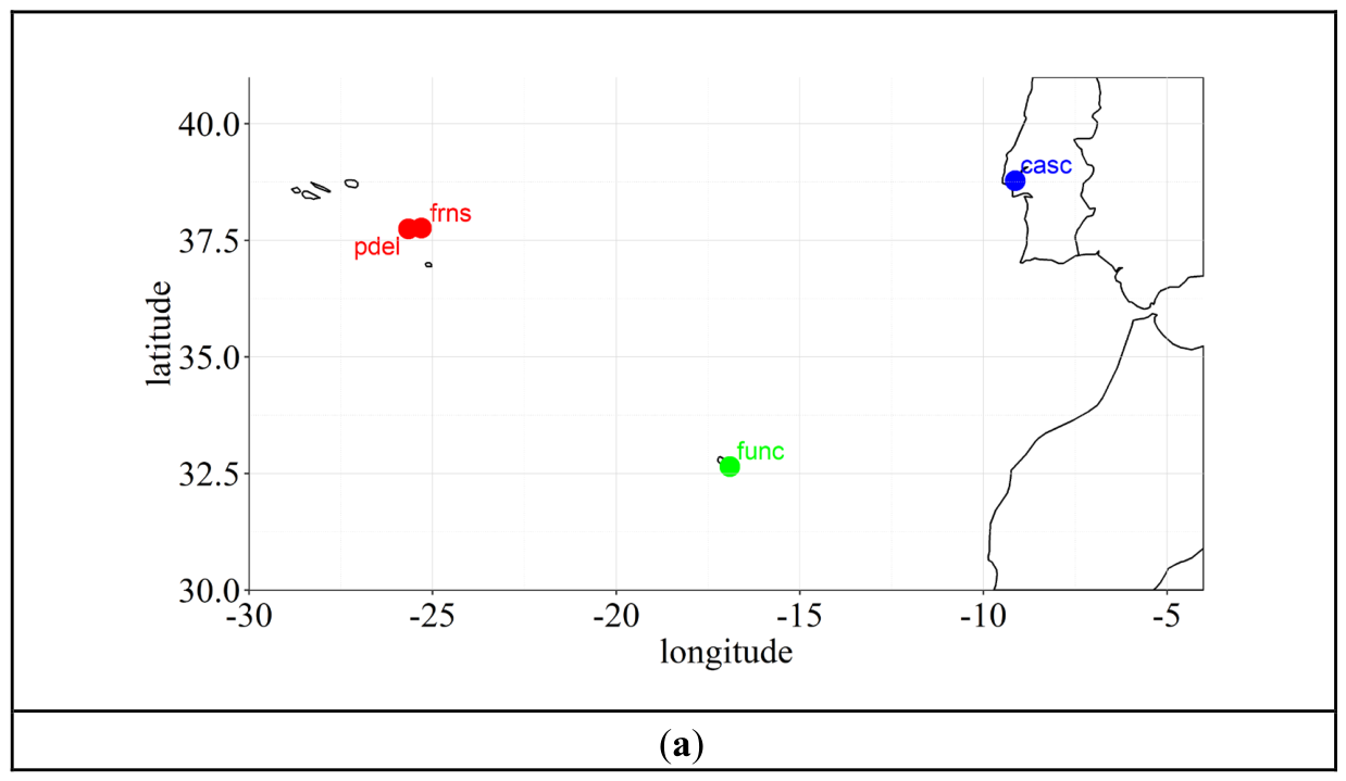
Figure 2.
Examples of different types of ionospheric disturbances. Top panels show Dst index variations during a particular event, bottom panels show ΔTEC variations at studied locations: Lisbon—green, Azores—blue, and Madeira—red. The types of the ΔTEC variations: (a) an absence of the statistically significant ionospheric disturbance (0-days-long or 0-type disturbance); (b) a 2-days-long ionospheric disturbance of the 0.p type; (c) a 3-days-long ionospheric disturbance of the 0.p.p type; (d) a 1-day long ionospheric disturbance of the p type; (e) a 2-days-long ionospheric disturbance of the p.p type; (f) a 2-days-long ionospheric disturbance of the p.n type; (g) a 1-day long ionospheric disturbance of the n type; (h) a 2-days-long ionospheric disturbance of the n.p type; (i) a 2-days-long ionospheric disturbance of the n.n type. Please note that these are examples of the ΔTEC variations, and not all plots contain the data for all three locations. Vertical lines separate days of the storm. Shaded blue area mark the ±2σ threshold (in case (i) the ±2σ threshold for Madeira is shown as a pink area additionally to the threshold for Lisbon and Azores shown in blue).
Figure 2.
Examples of different types of ionospheric disturbances. Top panels show Dst index variations during a particular event, bottom panels show ΔTEC variations at studied locations: Lisbon—green, Azores—blue, and Madeira—red. The types of the ΔTEC variations: (a) an absence of the statistically significant ionospheric disturbance (0-days-long or 0-type disturbance); (b) a 2-days-long ionospheric disturbance of the 0.p type; (c) a 3-days-long ionospheric disturbance of the 0.p.p type; (d) a 1-day long ionospheric disturbance of the p type; (e) a 2-days-long ionospheric disturbance of the p.p type; (f) a 2-days-long ionospheric disturbance of the p.n type; (g) a 1-day long ionospheric disturbance of the n type; (h) a 2-days-long ionospheric disturbance of the n.p type; (i) a 2-days-long ionospheric disturbance of the n.n type. Please note that these are examples of the ΔTEC variations, and not all plots contain the data for all three locations. Vertical lines separate days of the storm. Shaded blue area mark the ±2σ threshold (in case (i) the ±2σ threshold for Madeira is shown as a pink area additionally to the threshold for Lisbon and Azores shown in blue).
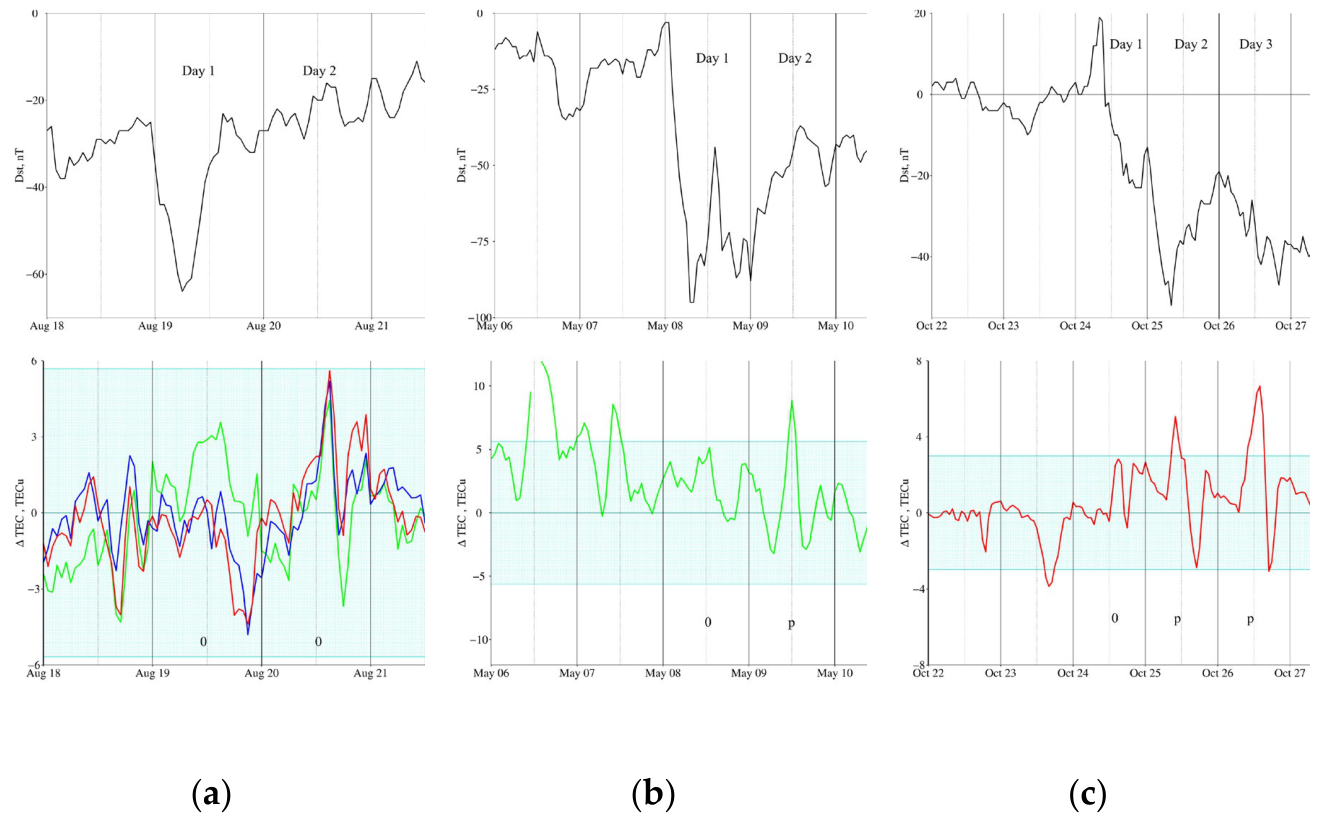
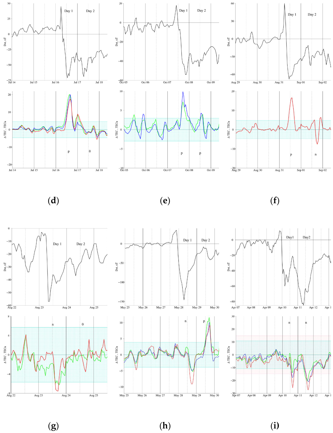
Figure 3.
Solar activity changes during the studied periods (monthly sunspot numbers).
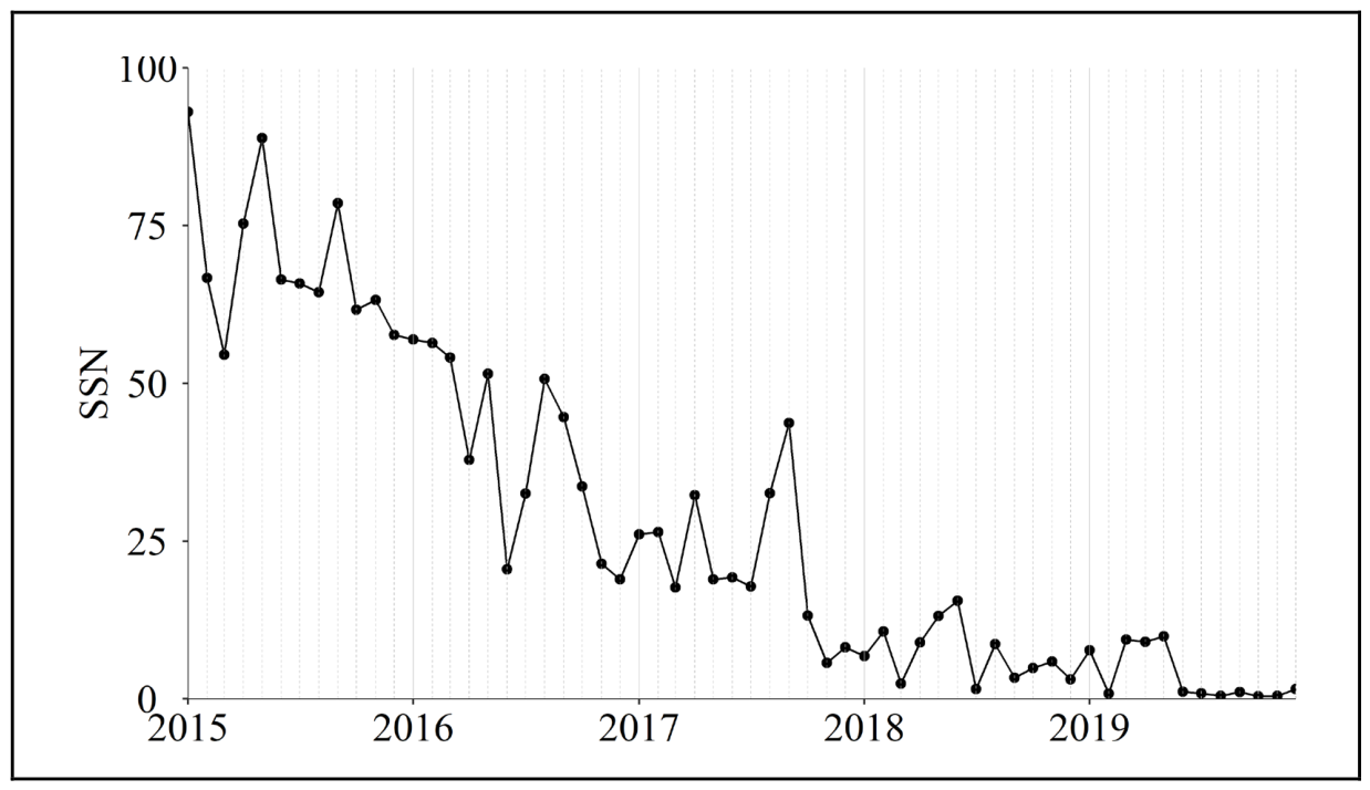
Table 1.
Coordinates of the GNSS receivers.
| Code | Name | Latitude | Longitude |
|---|---|---|---|
| CASC | Lisbon/Cascais, Continent | 38.7ºN | 9.14ºW |
| FRNS1 | Furnas, Azores/S. Miguel |
37.8ºN | 25.4ºW |
| PDLE2 | Ponta Delgada, Azores/S. Miguel | 37.8ºN | 25.8ºW |
| FUNC | Funchal, Madeira |
32.7ºN | 16.9ºW |
1 Data is available for January-June 2015, 2017-2019. 2 Data is available for July 2015–December 2016.
Disclaimer/Publisher’s Note: The statements, opinions and data contained in all publications are solely those of the individual author(s) and contributor(s) and not of MDPI and/or the editor(s). MDPI and/or the editor(s) disclaim responsibility for any injury to people or property resulting from any ideas, methods, instructions or products referred to in the content. |
© 2026 by the authors. Licensee MDPI, Basel, Switzerland. This article is an open access article distributed under the terms and conditions of the Creative Commons Attribution (CC BY) license (http://creativecommons.org/licenses/by/4.0/).
Copyright: This open access article is published under a Creative Commons CC BY 4.0 license, which permit the free download, distribution, and reuse, provided that the author and preprint are cited in any reuse.


