

Submitted:
14 July 2026
Posted:
14 July 2026
You are already at the latest version
Abstract
Cancer incidence exhibits substantial spatial disparities linked to environmental, behavioral, built-environment, healthcare-access, and socioeconomic conditions, yet the spatial scales at which these relationships operate remain insufficiently understood. This study develops an explainable spatial epidemiology workflow that integrates Random Forest, SHapley Additive exPlanations (SHAP), Ordinary Least Squares (OLS), Geographically Weighted Regression (GWR), and Multiscale Geographically Weighted Regression (MGWR) to examine county-level incidence for all-site, colon, breast, and skin cancers across Texas, USA. Random Forest and SHAP were used to identify outcome-specific nonlinear predictor relevance, and OLS, GWR, and MGWR were used to compare global, local, and multiscale spatial associations before and after RF-SHAP feature screening. MGWR generally achieved higher model fit than OLS and GWR. Before RF-SHAP screening, MGWR R² values were 0.701 for all-site cancer, 0.516 for colon cancer, 0.499 for breast cancer, and 0.694 for skin cancer, compared with OLS R² values of 0.343, 0.338, 0.257, and 0.368. RF-SHAP reduced predictors by about one-half and consistently improved AICc. The results show that environmental exposures, activity-related conditions, transportation access, screening, food insecurity, and chronic health indicators contribute to spatial differences in cancer incidence. The framework links nonlinear machine-learning evidence with spatially explicit interpretation for transferable epidemiological analysis.
Keywords:
cancer incidence
; explainable machine learning
; multiscale geographically weighted regression
; spatial heterogeneity
; environmental exposure
1. Introduction
Cancer remains a leading cause of mortality in the United States, with persistent and pronounced geographic disparities in incidence and outcomes [1,2]. These disparities are associated with a complex set of environmental exposures, built environment characteristics, healthcare-access conditions, socioeconomic vulnerabilities, and behavioral factors that vary across communities [3,4]. Long-term exposure to air pollutants such as PM₂.₅ and ozone, as well as climatic stressors such as extreme heat, has been linked to cancer-related risk through pathways involving chronic inflammation, oxidative stress, and cumulative environmental burden [5,6,7]. In addition, physical inactivity and limited access to supportive built environment features, such as sidewalks, bike lanes, and walkable neighborhoods, are associated with multiple cancers, particularly colon cancer [8,9]. Understanding how these environmental, behavioral, and contextual factors are associated with cancer incidence across space is important for informing place-based public health strategies.
Although research on environmental and behavioral determinants of cancer is growing, many studies rely on global regression frameworks that assume spatially constant relationships, potentially obscuring geographic variation in effect strength or direction. Geographically Weighted Regression (GWR) and Multiscale Geographically Weighted Regression (MGWR) address this limitation by allowing relationships to vary across space and, in the case of MGWR, to operate at variable-specific spatial scales [10,11,12]. However, MGWR applications in cancer research often rely on predefined sets of predictors and may not systematically address high-dimensional inputs, correlated contextual variables, or potential nonlinear relationships. In contrast, machine learning approaches such as Random Forest (RF) can handle complex predictor spaces and nonlinear effects, but they often lack direct spatial interpretability [13,14]. Explainable artificial intelligence methods, particularly SHapley Additive exPlanations (SHAP), can partially address this limitation by identifying the relative contribution, direction, and nonlinear behavior of predictors in machine-learning models [15]. However, SHAP alone does not explain whether predictor effects vary geographically or operate at different spatial scales. This gap highlights the need for analytical approaches that connect explainable machine-learning evidence with spatial regression modeling.
To address this need, this study develops and evaluates an explainable spatial epidemiology workflow that combines RF and SHAP (called RF-SHAP), and spatial regression models. RF is used as a nonlinear screening model to identify candidate environmental, behavioral, built-environment, healthcare-access, and socioeconomic predictors for each cancer outcome. SHAP values are then used to interpret predictor contributions and support transparent feature selection. The selected predictors are subsequently entered into OLS, GWR, and MGWR models to evaluate global associations, local spatial variation, and multiscale spatial heterogeneity. This workflow is designed not to replace spatial regression with machine learning, but to use explainable machine learning to guide spatial model construction and interpretation. This framing is important because variable selection in geographically weighted modeling has already been addressed by integrated penalized GWR methods, including Geographically Weighted Lasso, Geographically Weighted Elastic Net, and L0-norm GWR [16,17,18]. These methods perform local variable selection within the GWR framework and are especially relevant when the primary goal is local sparse linear modeling. The present study differs from these approaches by focusing on the integration of nonlinear explainable machine-learning evidence with MGWR-based spatial-scale interpretation. Therefore, the contribution of this study is not a new penalized geographically weighted estimator, but an applied and reproducible workflow for linking nonlinear predictor contribution, spatial variation, and multiscale interpretation in cancer incidence analysis.
This study contributes to existing literature in three ways. First, rather than relying solely on predefined variables, it introduces an explainable machine-learning-based feature-screening process using RF-SHAP prior to spatial modeling. Second, it applies OLS, GWR, and MGWR as benchmark models to evaluate whether RF-SHAP-selected predictors improve model parsimony and complexity-adjusted spatial model performance. Third, it uses MGWR to examine whether selected environmental, behavioral, built environment, and contextual predictors operate at different spatial scales across Texas counties. Unlike a simple concatenation of machine learning and spatial regression, each component of the workflow serves a distinct analytical role: RF captures nonlinear predictive relevance, SHAP explains predictor contributions, OLS provides a global baseline, GWR evaluates local spatial variation, and MGWR identifies variable-specific spatial scales.
Texas counties serve as a relevant case study due to their substantial environmental gradients, urban–rural contrasts in air pollution and heat exposure, and wide variation in behavioral, healthcare-access, and socioeconomic conditions. Using county-level data, this study examines four cancer outcomes (all-site, breast, colon, and skin cancer) three cancer outcomes, including overall cancer incidence, breast cancer incidence, and colon cancer incidence, to identify spatial patterns and associated factors. The results should be interpreted as population-level associations specific to this study context, rather than individual-level causal effects.
The objectives of this study are threefold: (1) to identify key environmental, behavioral, built-environment, and contextual predictors associated with cancer incidence using RF -SHAP-based feature screening; (2) to quantify and map spatial heterogeneity in these associations using GWR and MGWR; and (3) to examine whether RF-SHAP-selected predictors improve the explainability and performance of spatial regression models compared with full-predictor OLS, GWR, and MGWR models. Through this before-and-after experimental comparison, the study evaluates whether explainable machine-learning-based screening provides measurable value for downstream spatial modeling.
The remainder of this paper is organized as follows. Section 2 reviews literature on environmental, behavioral, and contextual determinants of cancer, geographically weighted modeling, penalized GWR variable-selection methods, and recent explainable machine-learning spatial workflows. Section 3 describes the data sources and preprocessing procedures. Section 4 details the analytical framework integrating RF, SHAP, OLS, GWR, and MGWR. Section 5 presents the model comparison results, RF-SHAP-selected predictors, and spatial patterns of associations. Section 6 discusses key findings, methodological implications, and the contribution of explainable machine learning to spatial cancer epidemiology. Section 7 concludes with study limitations and directions for future research.
2. Literature Review
Environmental exposures embedded within both natural and built environments are increasingly recognized as important determinants of cancer risk. Among natural exposures, ambient air pollution is one of the most extensively studied. Outdoor air pollution, and particularly fine particulate matter (PM₂.₅), has been classified as carcinogenic to humans by the International Agency for Research on Cancer [19]. Numerous cohort studies and meta-analyses have reported associations between long-term PM₂.₅ exposure and lung cancer incidence and mortality, with adverse effects observed even at relatively low concentrations [5,20,21]. Ozone (O₃), another widespread pollutant, has shown less consistent associations with cancer incidence, but it may contribute to oxidative stress pathways that indirectly affect cancer-related risk [6].
Thermal stress and extreme heat are also emerging environmental concerns in cancer-related research. Although direct evidence linking long-term heat exposure to cancer incidence remains limited, recent studies indicate that heatwaves can disrupt cancer care delivery, exacerbate treatment-related toxicities, and increase hospitalization and mortality risks among cancer patients [22,23]. Chronic heat exposure may also amplify physiological stress and interact with other environmental hazards, thereby compounding population-level vulnerability. As climate extremes intensify, understanding how heat and other environmental exposures contribute to spatial disparities in cancer-related outcomes has become increasingly important.
The built environment influences cancer risk through behavioral, accessibility, and exposure-related pathways. Neighborhood design characteristics, including land-use mix, density, street connectivity, and access to active transportation infrastructure, shape opportunities for physical activity and influence obesity, sedentary behavior, and exposure to traffic-related pollution. Large cohort studies have shown that higher walkability is associated with lower incidence of obesity-related cancers, including breast, endometrial, and ovarian cancers [24,25]. Physical inactivity has also been consistently associated with elevated risk for several cancers, especially colon cancer [8,9]. Collectively, these findings suggest that natural environmental exposures, built environment characteristics, and behavioral conditions jointly shape the spatial distribution of cancer incidence.
The spatial heterogeneity of cancer outcomes has motivated the use of geographically explicit modeling approaches. Geographically Weighted Regression (GWR) is a local spatial modeling method that estimates location-specific coefficients, allowing relationships between predictors and outcomes to vary across space rather than assuming spatial stationarity [26,27]. Its multiscale extension, Multiscale Geographically Weighted Regression (MGWR), further advances this framework by allowing each explanatory variable to operate at its own spatial bandwidth [11,12]. This is particularly relevant for environmental health research because different determinants may influence cancer outcomes at different geographic scales. For example, regional air pollution or climate-related exposures may operate across broad areas, whereas walkability, active transportation infrastructure, screening access, and healthcare barriers may vary more locally.
Recent cancer-focused spatial studies demonstrate the value of geographically weighted modeling for identifying spatially varying health relationships. Soleimani et al. [28] used geospatial methods, including GWR and spatial autocorrelation analysis, to examine breast cancer incidence in Iran and identified geographic patterns associated with sociodemographic, healthcare, environmental, and air-quality factors. Lal et al. [29] examined colorectal cancer diagnosis in Ohio and used GWR to show that the association between screening and early-stage diagnosis varied geographically; their results suggested that structural barriers such as uninsurance and transportation dependence may disrupt the screening-to-diagnosis pathway. Liu et al. [30] applied MGWR to prostate cancer incidence in the United States and showed that MGWR outperformed OLS and GWR while revealing variable-specific spatial bandwidths and regionally differentiated coefficient patterns. These studies indicate that cancer-related determinants do not necessarily operate uniformly across space and that spatially explicit methods can provide useful insights for geographically targeted public health strategies.
Despite these strengths, standard GWR and MGWR have several methodological limitations. Both are generally based on local linear and additive assumptions, limiting their ability to capture nonlinearities, threshold effects, and complex interactions that are common in environmental and behavioral health processes. In addition, GWR and MGWR do not inherently perform variable selection. This limitation is important when studies include many environmental, behavioral, built-environment, healthcare-access, and socioeconomic predictors, many of which may be conceptually related or statistically correlated. Local multicollinearity can make geographically weighted coefficients unstable and difficult to interpret, even when global multicollinearity diagnostics appear acceptable [16,31].
Methodological research has extended GWR to address variable selection, local collinearity, and coefficient instability. Wheeler [16] proposed Geographically Weighted Lasso (GWL), which embeds an L1 penalty within GWR to shrink local coefficients and perform location-specific variable selection. Li and Lam [17] further developed Geographically Weighted Elastic Net (GWEN), combining L1 and L2 penalties to improve variable selection while stabilizing coefficient estimates under multicollinearity. More recently, Wu et al. [18] introduced an L0-norm variable adaptive GWR approach that directly constrains the number of nonzero local coefficients and supports local subset selection. Collectively, these studies demonstrate that variable selection under spatial variation has been extensively examined and that integrated local variable-selection methods already exist. However, these approaches remain primarily local linear models designed to improve coefficient sparsity, stability, and multicollinearity control. They do not directly address nonlinear predictive relationships, interaction effects, or SHAP-based explainable machine-learning interpretation. Therefore, while GWL, GWEN, and L0-GWR provide important methodological benchmarks, they address a different research objective from the present study, which focuses on linking nonlinear predictor contributions from RF-SHAP with GWR/MGWR-based spatial heterogeneity and scale interpretation.
Machine learning methods provide a complementary perspective for environmental health and cancer spatial epidemiology. Tree-based models such as RF and XGBoost can capture nonlinear relationships and interaction effects among environmental, behavioral, built-environment, healthcare-access, and socioeconomic predictors [13,32]. In cancer research, Lal et al. [29] used Variable Selection Using RF to identify structural predictors of early-stage colorectal cancer diagnosis, while Ferrete and Raposo [33] applied RF, Geographical RF, and Shapley-value interpretation to analyze breast cancer mortality inequalities in Brazil. These studies demonstrate that machine learning can help identify complex and nonlinear predictor relevance in cancer-related outcomes, especially when many contextual variables are considered. However, machine learning models are often prediction-oriented and may lack direct spatial interpretability. RF can rank predictors by importance, but conventional feature-importance measures do not fully explain the direction, magnitude, or nonlinear form of each predictor’s contribution.
Explainable machine-learning methods, particularly SHapley Additive exPlanations (SHAP), have increasingly been used to interpret complex nonlinear models by estimating each predictor’s contribution to model predictions [15]. In spatial and environmental research, recent studies have combined SHAP-based machine learning with geographically weighted models to link global nonlinear interpretation with local spatial effects. For example, Jeong et al. [34] used XGBoost-SHAP and GWR to examine land surface temperature in Korean megacities, showing that SHAP identified globally important nonlinear drivers while GWR revealed spatially varying local effects. Arifullah et al. [35] integrated XGBoost, SHAP, GWR, and spatial autocorrelation analysis to examine groundwater depletion, using SHAP to identify nonlinear driver contributions and GWR to uncover local heterogeneity. Similarly, Song et al. [36] combined XGBoost-SHAP and MGWR to analyze ecosystem-service drivers, demonstrating that SHAP can support driver identification while MGWR reveals spatially varying effects and variable-specific spatial scales.
These studies show that SHAP-based machine learning and geographically weighted models can serve complementary roles: SHAP helps identify nonlinear predictor importance, interaction effects, and threshold-like patterns, whereas GWR and MGWR provide spatially explicit interpretation through local coefficients and, in the case of MGWR, variable-specific bandwidths. However, SHAP does not directly estimate spatially varying regression relationships, and GWR/MGWR remain limited by local linear assumptions. Moreover, many existing ML, SHAP, GWR/MGWR studies emphasize interpretation rather than systematically testing whether SHAP-supported feature screening improves downstream spatial model performance. This gap is especially relevant in cancer spatial epidemiology, where GWR and MGWR studies have examined spatial heterogeneity and machine-learning studies have identified important health or socioeconomic predictors, but relatively few studies have evaluated whether explainable machine-learning-based feature screening improves the parsimony and complexity-adjusted performance of spatial cancer models.
3. Materials and Methods
3.1. Study Area
The study focuses on Texas, encompassing all 254 counties as the unit of analysis. Texas provides a useful case study for examining spatial variation in environmental and behavioral factors due to its pronounced geographic, climatic, and socioeconomic diversity. The state includes highly urbanized regions with dense transportation networks as well as rural areas with limited infrastructure, resulting in substantial variation in environmental exposures, physical activity opportunities, and population health outcomes. County-level spatial resolution is appropriate for this analysis because it aligns with administrative units commonly used in public health planning and environmental management. Accordingly, the results are interpreted as population-level associations intended to inform regional patterns rather than individual-level relationships.
3.2. Cancer Incidence Data
County-level cancer incidence data were obtained from the National Cancer Institute State Cancer Profiles. This dataset provides age-adjusted incidence rates per 100,000 population, offering a standardized measure across counties. The analysis focuses on four outcomes: all-site cancer, breast cancer, colon cancer, and skin cancer. These cancer types were selected based on their prevalence and their potential associations with environmental exposures and behavioral factors. The temporal coverage spans 2015–2020, and all variables are aggregated at the county level. The outcomes are treated as population-level indicators of cancer incidence, and the analysis focuses on identifying spatial patterns of association rather than individual-level risk relationships.
3.3. Environmental and Physical Activity Exposures
This study integrates multiple environmental and behavioral indicators that are associated with cancer incidence in prior research. Environmental variables were derived from the Centers for Disease Control and Prevention (CDC) Environmental Public Health Tracking Network and related federal datasets [37]. These include annual average concentrations of fine particulate matter (PM₂.₅) and ground-level ozone (O₃), long-term mean heat index, ultraviolet (UV) radiation intensity, and additional indicators such as emissions and water coverage. These variables were aggregated to the county level and standardized using z-score normalization to ensure comparability across spatial units.
Behavioral and built environment indicators were obtained from the CDC PLACES Project and the Strava Metro platform [38,39]. Variables include the proportion of adults reporting no leisure-time physical activity (No_LeisureTime_PA), aerobic activity levels, and measures of walking and cycling activity (Walk_n, Bike_n), along with built environment indicators such as bike lane infrastructure and walkability indices.
Several of these datasets have known limitations. PLACES indicators are derived from self-reported survey data and modeled small-area estimates, which may introduce bias reporting and estimation uncertainty. Strava Metro data are subject to selection bias, as users are not representative of the general population and tend to be younger, more affluent, and concentrated in urban areas. As a result, these variables are interpreted as proxies for relative activity patterns rather than precise measures of population-level behavior. When aggregated to the county level, these indicators provide useful comparative information on spatial variation, but their limitations should be considered when interpreting results. Accordingly, these variables are used as proxy indicators of relative spatial variation in activity-related conditions, rather than unbiased or precise measures of true population behavior, and their interpretation is limited to comparative ecological patterns.
3.4. Temporal Alignment of Data
A limitation of the input data relates to temporal alignment across datasets. Cancer incidence rates were aggregated over the period 2015–2020, while behavioral and built environment variables primarily reflect conditions from 2018–2020. In contrast, environmental variables such as air pollution and climatic indicators were represented using long-term averages to capture sustained exposure conditions. This temporal inconsistency arises from differences in data availability across sources and is common in ecological studies that integrate multiple datasets. To address this issue, all predictors are treated as approximations of prevailing conditions during the broader study period, under the assumption that key environmental and socioeconomic patterns change gradually over time. Nevertheless, the temporal correspondence between exposures and outcomes may not fully reflect the true latency of cancer development, and results should be interpreted accordingly.
3.5. Health Behaviors, Screening, and Social Determinants
To better contextualize environmental and behavioral associations, the analysis incorporates additional indicators of health behaviors, screening, and broader social determinants of health. These include cancer screening prevalence (breast and colorectal), as well as lifestyle-related factors such as obesity, smoking, and cholesterol screening. In addition, indicators of social and structural conditions, such as food insecurity, housing insecurity, transportation access, and mobility limitations, are included to capture broader contextual influences on population health. These variables reflect non-medical drivers of health that may shape both exposure and vulnerability across regions. Their inclusion helps account for potential confounding factors, although unmeasured influences may still remain.
3.6. Data Preprocessing and Normalization
All datasets were integrated at the county level using standardized Federal Information Processing Standard (FIPS) codes to ensure spatial alignment. Environmental and behavioral variables were standardized using z-score normalization to improve comparability.
Multicollinearity was assessed using the Variance Inflation Factor (VIF), and highly collinear variables were excluded to improve model stability. While this process reduces redundancy among predictors, some degree of correlation among conceptually related variables may persist and should be considered in interpretation. Missing values were minimal and were imputed using mean values. These preprocessing steps resulted in a harmonized dataset suitable for machine learning–based screening and spatial regression analysis.
Table 1 summarizes the outcome variables, predictor variables, and spatial coordinates used in the analysis. It provides variable names, analytical role, base code, and a concise definition to improve transparency and help readers understand how each attribute was interpreted in the RF/SHAP, OLS, GWR, and MGWR modeling workflow.
4. Analytical Framework
This study integrates explainable machine-learning-based feature screening with spatial regression to examine associations between environmental, behavioral, built-environment, healthcare-access, and socioeconomic factors and cancer incidence across Texas counties. The analytical workflow consists of three main stages. First, RF models are trained separately for each cancer outcome to identify predictors with potential nonlinear and interaction-based relevance. Second, SHAP is used to interpret predictor contributions and rank variables according to their relative importance. Third, the RF-SHAP-selected predictors are incorporated into Ordinary Least Squares (OLS), Geographically Weighted Regression (GWR), and Multiscale Geographically Weighted Regression (MGWR) models to evaluate global associations, local spatial variation, and multiscale spatial heterogeneity. This framework is designed to balance dimensionality reduction, flexibility in variable screening, and interpretability of spatial patterns, with an emphasis on exploratory analysis rather than causal inference. Figure 1 structures the framework for this study.
4.1. Baseline Global Model: Ordinary Least Squares (OLS)
Ordinary Least Squares (OLS) regression serves as a baseline global model to estimate linear associations between predictor variables and county-level cancer incidence rates. OLS assumes spatial stationarity, meaning that coefficients are constant across all locations. While this assumption may not hold in heterogeneous environments, OLS provides a useful benchmark for evaluating improvements from spatially explicit models. Model performance was assessed using the coefficient of determination (R²) and the corrected Akaike Information Criterion (AICc).
4.2. Random Forest and SHAP based Feature Screening
RF regression was used as a complementary modeling approach to identify predictors potentially associated with nonlinear relationships and interactions. As a nonparametric ensemble method, RF constructs multiple decision trees and aggregates their predictions to improve robustness and predictive performance [13]. Model performance was evaluated using out-of-bag (OOB) R² and root mean squared error (RMSE). Figure 2 and Figure 3 present the RF/SHAP feature-screening results, including SHAP summary plots for the cancer outcomes and Random Forest feature-importance plots showing the top 15 selected predictors.
SHAP was then used to interpret the RF models and quantify the contribution of each predictor to model predictions [15]. For each predictor, mean absolute SHAP values were calculated to measure its overall contribution to prediction. Predictors with higher mean absolute SHAP values were interpreted as having greater predictive relevance in the RF model. SHAP summary and dependence plots were used to examine whether predictors had positive, negative, nonlinear, or threshold-like relationships with predicted cancer incidence.
Based on the SHAP rankings, outcome-specific predictor subsets were selected for spatial regression. This procedure replaced the earlier Lasso-based screening step. The purpose of SHAP-based selection was not to identify causal predictors, but to provide a transparent and explainable basis for reducing the candidate predictor set before OLS, GWR, and MGWR modeling.
4.3. Relationship Between Random Forest, SHAP, and Spatial Regression
RF, SHAP, OLS, GWR, and MGWR serve distinct but complementary roles in the analytical framework. RF identifies variables that may be relevant through nonlinear or interaction-based relationships. SHAP explains how each predictor contributes to RF predictions and provides a transparent basis for feature screening. OLS estimates global associations, GWR evaluates whether relationships vary locally across space, and MGWR further identifies whether different predictors operate at different spatial scales.
This sequential design is intended to avoid treating machine learning and spatial regression as interchangeable models. Instead, RF-SHAP provides nonlinear predictive evidence, while GWR and MGWR provide spatial explanatory evidence. Variables selected by RF-SHAP are treated as candidate predictors for spatial modeling rather than as definitive causal determinants. The spatial models then evaluate whether these selected variables exhibit spatially varying associations and, in the case of MGWR, variable-specific spatial bandwidths.
4.4. Geographically Weighted Regression and MGWR
Geographically Weighted Regression (GWR) and Multiscale Geographically Weighted Regression (MGWR) were applied to model spatially varying relationships between cancer incidence and selected predictors. GWR estimates location-specific coefficients using a single bandwidth for all variables, while MGWR extends this framework by allowing each predictor to operate at its own spatial scale.
MGWR can be expressed as:
where is the bandwidth associated with the th covariate. MGWR employs a backfitting algorithm that iteratively updates variable-specific bandwidths to minimize information criteria such as AICc, yielding an optimal spatial scale for each covariate [12,40].
In MGWR, bandwidths were calibrated separately for each predictor using an AICc-based optimization procedure within an iterative backfitting framework. Specifically, the model iteratively estimates local coefficients while optimizing variable-specific bandwidths, allowing each predictor to operate at its own spatial scale. An adaptive kernel was used to account for variation in spatial distribution across counties. Bandwidths were selected by minimizing the corrected Akaike Information Criterion (AICc), and the optimization process employed a search algorithm (e.g., golden section search) to efficiently identify optimal bandwidths. The iterative procedure continued until convergence, defined as minimal change in AICc and parameter estimates between successive iterations. This approach enables MGWR to distinguish between processes operating at broader regional scales (e.g., environmental exposures) and those varying at more localized scales (e.g., built environmental features).
4.5. Hierarchical (Mixed-Effects) Model for Comparison
To provide a comparison with alternative advanced modeling approaches, a hierarchical (mixed effects) model was implemented as a representative multilevel framework. The model includes fixed effects for all selected predictors and random intercepts defined at a regional grouping level to account for unobserved heterogeneity across spatial clusters. The hierarchical model can be expressed as:
where stands for cancer incidence in county within region , represents the value of predictor for county in region , stands for global intercept, are the fixed effects (global coefficients), stands for random intercept for region and is the residual error. Regions were defined based on spatial grouping of counties to reflect broader geographic structure. This model provides a contrast to MGWR by allowing grouped heterogeneity but assuming globally constant fixed effects, whereas MGWR explicitly models spatially varying relationships at multiple scales.
4.6. Model Evaluation and Diagnostics
To evaluate whether RF-SHAP feature screening improved downstream spatial modeling, each cancer outcome was modeled under two experimental conditions. First, OLS, GWR, and MGWR were estimated to use the full candidate predictor set. Second, the same models were estimated using the RF-SHAP-selected predictor set. This before-and-after design allowed direct comparison of model performance before and after explainable machine-learning-based feature screening. The comparison focused on three questions. First, do RF-SHAP reduce the number of predictors and improve model parsimony? Second, do RF-SHAP-selected predictors improve complexity-adjusted model performance, particularly AICc, in GWR and MGWR? Third, do RF-SHAP predictors preserve meaningful spatial interpretation through GWR coefficients and MGWR bandwidths?
The benchmark models were therefore:
- OLS with full predictors
- GWR with full predictors
- MGWR with full predictors
- OLS with RF-SHAP -selected predictors
- GWR with RF-SHAP -selected predictors
- MGWR with RF-SHAP -selected predictors
This experimental structure was designed to determine whether the RF-SHAP step contributed measurable value beyond simply adding a machine-learning model to the workflow.
Model performance was compared across OLS, GWR, and MGWR using R², RMSE, AIC, and AICc where applicable. For GWR and MGWR, AICc was emphasized because it accounts for both model fit and model complexity, making it especially useful for comparing full-predictor and RF-SHAP-selected models. A reduction in AICc after RF-SHAP selection was interpreted as evidence that the selected predictor set improved model parsimony and complexity-adjusted performance.
4.7. Methodological Considerations
Several methodological considerations should be noted. First, although RF-SHAP can identify nonlinear predictor contributions, GWR and MGWR estimate spatially varying linear associations. Therefore, MGWR coefficients should be interpreted as local linear approximations of potentially more complex relationships identified in the machine-learning stage. Second, SHAP values quantify predictor contributions to RF predictions, but they do not estimate causal effects or spatially varying regression coefficients. Therefore, SHAP results and MGWR results provide complementary evidence: SHAP identifies nonlinear predictive relevance, while MGWR evaluates spatial heterogeneity and variable-specific spatial scales. Third, RF-SHAP-based feature screening is a sequential rather than fully integrated modeling strategy. Variables identified as important in a global machine-learning model may not always exhibit strong or consistent local spatial associations. For this reason, the study compares full-predictor and RF-SHAP-selected OLS, GWR, and MGWR models rather than assuming that RF-SHAP-selected variables automatically improve spatial model performance. Fourth, multicollinearity among conceptually related predictors may still affect coefficient stability in GWR and MGWR, even after feature screening. As a result, coefficient estimates should be interpreted cautiously, especially for variables representing overlapping constructs such as physical activity, built environment, healthcare access, and socioeconomic vulnerability. Finally, because the study uses county-level ecological data, all results should be interpreted as population-level associations rather than individual-level risks or causal effects.
5. Results
5.1. Model Performance Before and After RF-SHAP Feature Screening
To evaluate whether RF-SHAP-based feature screening improved the downstream spatial modeling workflow, model performance was compared before and after feature selection for four cancer outcomes: overall cancer incidence, colon cancer incidence, breast cancer incidence, and skin cancer incidence. For each outcome, OLS, GWR, and MGWR were first estimated using the full candidate predictor set and then re-estimated using the RF-SHAP-selected predictor set. This before-and-after comparison was designed to assess whether the explainable machine-learning step improved model parsimony and complexity-adjusted fit rather than simply increasing in-sample explanatory power.
RF-SHAP feature screening substantially reduced model dimensionality across all four outcomes. The number of predictors decreased from 45 to 24 for overall cancer incidence, from 47 to 24 for colon cancer, from 48 to 24 for breast cancer, and from 46 to 22 for skin cancer. This reduction indicates that RF-SHAP removed approximately half of the original predictors while retaining outcome-specific variables for subsequent spatial modeling.
Table 1 summarizes the model comparison results. Across all four cancer outcomes, the RF-SHAP-selected models generally showed lower R² values than the full-predictor models, which is expected because the reduced models used substantially fewer predictors. However, AICc improved consistently after RF-SHAP feature screening for OLS, GWR, and MGWR. This pattern suggests that the RF-SHAP-selected models provided a better balance between model fit and complexity.

Table 2.
Model performance before and after RF-SHAP-based feature screening.
| Cancer outcome | Stage | Model | No. predictors | R² | AICc | ΔR² | ΔAICc |
|---|---|---|---|---|---|---|---|
| Overall incidence | Before RF-SHAP | OLS | 45 | 0.343 | 730.106 | — | — |
| Overall incidence | Before RF-SHAP | GWR | 45 | 0.538 | 733.027 | — | — |
| Overall incidence | Before RF-SHAP | MGWR | 45 | 0.701 | 756.895 | — | — |
| Overall incidence | After RF-SHAP | OLS | 24 | 0.281 | 695.376 | -0.062 | -34.730 |
| Overall incidence | After RF-SHAP | GWR | 24 | 0.424 | 682.005 | -0.114 | -51.022 |
| Overall incidence | After RF-SHAP | MGWR | 24 | 0.599 | 694.515 | -0.102 | -62.380 |
| Colon cancer | Before RF-SHAP | OLS | 47 | 0.338 | 744.423 | — | — |
| Colon cancer | Before RF-SHAP | GWR | 47 | 0.487 | 781.281 | — | — |
| Colon cancer | Before RF-SHAP | MGWR | 47 | 0.516 | 752.527 | — | — |
| Colon cancer | After RF-SHAP | OLS | 24 | 0.242 | 708.627 | -0.096 | -35.796 |
| Colon cancer | After RF-SHAP | GWR | 24 | 0.404 | 703.879 | -0.083 | -77.402 |
| Colon cancer | After RF-SHAP | MGWR | 24 | 0.397 | 715.825 | -0.119 | -36.702 |
| Breast cancer | Before RF-SHAP | OLS | 48 | 0.257 | 770.659 | — | — |
| Breast cancer | Before RF-SHAP | GWR | 48 | 0.426 | 803.427 | — | — |
| Breast cancer | Before RF-SHAP | MGWR | 48 | 0.499 | 765.489 | — | — |
| Breast cancer | After RF-SHAP | OLS | 24 | 0.190 | 725.462 | -0.067 | -45.197 |
| Breast cancer | After RF-SHAP | GWR | 24 | 0.287 | 737.004 | -0.139 | -66.423 |
| Breast cancer | After RF-SHAP | MGWR | 24 | 0.428 | 721.835 | -0.071 | -43.654 |
| Skin cancer | Before RF-SHAP | OLS | 46 | 0.368 | 723.164 | — | — |
| Skin cancer | Before RF-SHAP | GWR | 46 | 0.492 | 761.274 | — | — |
| Skin cancer | Before RF-SHAP | MGWR | 46 | 0.694 | 749.993 | — | — |
| Skin cancer | After RF-SHAP | OLS | 22 | 0.241 | 704.013 | -0.127 | -19.151 |
| Skin cancer | After RF-SHAP | GWR | 22 | 0.358 | 702.312 | -0.134 | -58.962 |
| Skin cancer | After RF-SHAP | MGWR | 22 | 0.484 | 671.419 | -0.210 | -78.574 |
Note: ΔR² and ΔAICc compare each RF-SHAP-selected model with the corresponding full-predictor model for the same cancer outcome and model type. Negative ΔAICc values indicate improved complexity-adjusted model performance after RF-SHAP feature screening.
For overall cancer incidence, RF-SHAP selection reduced the predictor set from 45 to 24. Although MGWR R² decreased from 0.701 to 0.599, MGWR AICc improved from 756.895 to 694.515. GWR also improved substantially, with AICc decreasing from 733.027 to 682.005. These results suggest that the full-predictor spatial models for overall incidence may have been over-parameterized and that RF-SHAP produced a more efficient predictor subset.
For colon cancer, the strongest post-selection spatial model was GWR rather than MGWR. RF-SHAP-selected GWR achieved R² = 0.404 and AICc = 703.879, compared with R² = 0.397 and AICc = 715.825 for RF-SHAP-selected MGWR. This suggests that colon cancer incidence may benefit from local spatial modeling, but the additional multiscale complexity of MGWR did not improve complexity-adjusted fit after feature selection. The largest AICc improvement for colon cancer was observed in GWR, where AICc decreased by 77.402 points.
For breast cancer, RF-SHAP-selected MGWR performed better than RF-SHAP-selected GWR. Although the reduced MGWR model had lower R² than the full-predictor MGWR model, it improved AICc by 43.654 points. This indicates that breast cancer associations retained a multiscale spatial component after feature screening, but also that county-level environmental and contextual variables explained less variation in breast cancer incidence than in overall or skin cancer models.
For skin cancer, RF-SHAP selection produced the largest AICc improvement in MGWR among the four outcomes. MGWR AICc decreased from 749.993 to 671.419, an improvement of 78.574 points. Although R² decreased from 0.694 to 0.484, the large AICc reduction suggests that RF-SHAP-selected MGWR provided a substantially more parsimonious model. This result supports the usefulness of combining explainable feature screening with multiscale spatial modeling for skin cancer incidence.
Figure 4 illustrates model performance across cancer types. Explanatory power varies by outcome, with relatively higher R² values observed for skin cancer and all-site cancer, followed by colon cancer, while breast cancer exhibits comparatively lower explanatory power. This pattern suggests that environmental and behavioral variables included in this study may be more strongly associated with certain cancer types than others. Figure 5 illustrates the spatially varying coefficients for no leisure-time physical activity in relation to colon cancer incidence. The association is positive across most counties, with stronger effects observed in eastern Texas. While the direction of the relationship is relatively consistent, the magnitude varies geographically, highlighting the importance of local context in shaping observed patterns.
5.2. RF-SHAP Predictor Screening and Outcome-Specific Feature Sets
The RF-SHAP results indicate that different cancer outcomes were associated with different predictor profiles. Rather than applying one fixed predictor set to all outcomes, RF-SHAP produced outcome-specific subsets that reflected different combinations of environmental, behavioral, built-environment, healthcare-access, and socioeconomic variables. This outcome-specific feature selection is important because overall cancer incidence, colon cancer, breast cancer, and skin cancer may reflect different etiological pathways and contextual influences.
RF was used as a nonlinear screening model rather than as the final explanatory model. SHAP values were then used to rank variables according to their contribution to RF predictions and to provide an interpretable basis for predictor selection. Therefore, the RF-SHAP stage should be interpreted as an exploratory screening and explanation step. Its purpose was to reduce dimensionality and identify candidate predictors for spatial regression, not to establish causal effects or replace spatial modeling.
The selected predictors differed across outcomes. Overall cancer incidence retained a mixture of environmental exposures, behavioral variables, access-related indicators, and built-environment measures. Colon cancer predictors emphasized physical health, physical inactivity, disability-related indicators, screening, smoking, diabetes, and transportation-related variables. Breast cancer predictors included screening-related indicators, population structure, food insecurity, transportation barriers, environmental exposures, obesity, and physical activity. Skin cancer predictors reflected a distinct combination of environmental, demographic, and contextual variables. These differences support the use of outcome-specific RF-SHAP screening before spatial modeling.
5.3. Spatial Model Comparison and Multiscale Interpretation
The spatial model comparison shows that GWR and MGWR provide complementary perspectives on geographic variation. GWR evaluates whether predictor–outcome relationships vary across counties using a single spatial bandwidth, while MGWR allows each predictor to operate at its own spatial scale. The results show that MGWR was not uniformly superior across all outcomes after feature screening. Instead, the preferred model depended on the cancer outcome and the balance between explanatory power and model complexity.
For overall cancer incidence, breast cancer, and skin cancer, the RF-SHAP-selected MGWR models provided important multiscale interpretation. These results suggest that selected predictors may operate at different geographic scales, with some associations reflecting broad regional patterns and others varying more locally. For colon cancer, the RF-SHAP-selected GWR model had the lowest AICc among the post-selection spatial models, suggesting that a single-scale local model may be more efficient for this outcome. This outcome-specific pattern is important for interpreting the workflow. The purpose of RF-SHAP selection was not to force MGWR to outperform all other models, but to evaluate whether explainable machine-learning-based feature screening could produce better estimators that can be used for regression models to analyze non-stationary relationships. The results show that RF-SHAP improved AICc across all OLS, GWR, and MGWR models but lower R2, while the best post-selection spatial model varied by outcome.
Overall, the results provide experimental evidence that RF-SHAP contributed measurable value to the spatial regression modeling workflow. Across all four cancer outcomes, RF-SHAP reduced the number of predictors by approximately one-half and improved AICc for every model comparison. Although R² values decreased after feature selection, this pattern reflects the reduced number of predictors and should be interpreted alongside the consistent improvements in AICc. The results therefore suggest that RF-SHAP improved model parsimony and complexity-adjusted fit rather than simply maximizing in-sample explanatory power.
These findings help address the concern that combining machine learning and spatial regression may represent simple model concatenation. In the workflow, each model component serves a distinct purpose: RF captures nonlinear predictive relevance, SHAP explains predictor contributions and supports transparent feature screening, OLS provides a global baseline, GWR evaluates geographic variation, and MGWR provides multiscale spatial interpretation. The before-and-after comparison demonstrates that the RF-SHAP step improved downstream spatial model efficiency and therefore provides empirical support for the analytical framework.
6. Discussion
This study examined spatial variation in associations between environmental, behavioral, built-environment, healthcare-access, socioeconomic factors, and cancer incidence across Texas counties using an explainable machine-learning and spatial regression workflow. The framework used RF and SHAP to identify outcome-specific predictor subsets, followed by OLS, GWR, and MGWR to evaluate global associations, geographic variation, and multiscale spatial patterns. Across the four cancer outcomes, RF-SHAP-based feature screening substantially reduced model dimensionality and improved the complexity-adjusted performance of OLS, GWR, and MGWR models.
Environmental exposures, particularly PM₂.₅ and heat index, exhibited relatively broad spatial patterns, suggesting that their associations with cancer incidence operate at regional scales. These findings are consistent with prior literature linking long-term air pollution exposure and climatic stressors to cancer-related outcomes. In contrast, behavioral and built environment variables, such as walkability and no leisure-time physical activity, demonstrated more localized patterns, indicating that their associations may be more sensitive to local context. These results highlight the importance of considering both regional and local processes when examining spatial patterns of cancer incidence.
6.1. Interpretation and Policy-Relevant Insights
The findings suggest that cancer incidence is associated with a combination of environmental, behavioral, built-environment, healthcare-access, and socioeconomic conditions that vary geographically across Texas counties. The RF-SHAP stage helped identify outcome-specific predictors with nonlinear or interaction-based relevance, while GWR and MGWR provided spatial interpretation of where and at what scale these associations appeared. Together, these results suggest that cancer-related geographic disparities are shaped by both broad regional exposures and more localized contextual conditions.
From a public health perspective, this distinction is important because different predictors may require different intervention scales. Environmental exposures such as air pollution, heat, emissions, ultraviolet radiation, and water-related conditions may require regional or cross-county strategies, including environmental monitoring, heat-mitigation planning, and air-quality management. In contrast, behavioral, built-environment, healthcare-access, and socioeconomic factors may be more actionable at the county or community level through interventions such as improved walkability, active transportation infrastructure, screening outreach, healthcare access, and support for socially vulnerable populations.
These implications should be interpreted cautiously. The analysis is ecological and does not establish individual-level risk or causal effects. Associations involving physical inactivity, screening, transportation barriers, or food insecurity may reflect broader structural conditions rather than direct causal pathways. Therefore, the results are best understood as spatial evidence for hypothesis generation, place-based prioritization, and future targeted research rather than as definitive policy prescriptions.
6.2. Variation Across Cancer Outcomes
The results also indicate that the usefulness of RF-SHAP-based feature screening and spatial modeling varied by cancer outcome. Overall cancer incidence and skin cancer showed relatively strong evidence that RF-SHAP-selected MGWR could preserve meaningful explanatory power while substantially improving model parsimony. This suggests that these outcomes may be more strongly associated with broad environmental and contextual conditions captured in the county-level dataset.
Colon cancer showed a different pattern. After RF-SHAP selection, GWR provided a more efficient post-selection model than MGWR, suggesting that colon cancer associations may be spatially variable but may not require the additional complexity of variable-specific MGWR bandwidths in this dataset. Substantively, this outcome was more closely linked with behavioral, health-status, screening, and transportation-related predictors, which is consistent with the role of physical activity, healthcare access, and preventive screening in colon cancer patterns.
Breast cancer showed comparatively lower explanatory performance, even after RF-SHAP-based feature screening. This is likely because breast cancer incidence is influenced by individual-level biological, reproductive, hormonal, genetic, and screening-related factors that are not fully represented in county-level environmental and contextual data. Therefore, the breast cancer findings should be interpreted more cautiously and viewed as population-level spatial associations rather than a comprehensive explanation of breast cancer risk.
6.3. Methodological Implications
A key methodological implication of this study is that RF-SHAP improved model parsimony and interpretability without requiring the study to claim a new spatial-statistical estimator. In the workflow, each component has a distinct analytical role. RF identifies nonlinear and interaction-based predictive relevance. SHAP explains predictor contributions and supports transparent feature screening. OLS provides a global baseline. GWR evaluates whether associations vary geographically. MGWR evaluates whether selected predictors operate at different spatial scales. This structure clarifies that the workflow is not a simple concatenation of methods but a sequence of complementary analytical steps.
The before-and-after comparison strengthens this methodological claim. Full-predictor models often achieved higher R², but they used substantially more predictors and produced worse AICc values. RF-SHAP-selected models used approximately half as many predictors and improved AICc across all OLS, GWR, and MGWR comparisons. This trade-off indicates that RF-SHAP helped reduce over-parameterization and improved the efficiency of downstream spatial models. For an ecological spatial epidemiology study with many correlated contextual predictors, improved AICc and parsimony are especially important because they support more interpretable and less overfit models.
At the same time, RF should not be interpreted as a final predictive model in this study. Its role is exploratory feature screening rather than definitive prediction. SHAP values quantify how predictors contribute to RF predictions, but they do not estimate causal effects or spatially varying regression coefficients. Conversely, GWR and MGWR estimate spatially varying linear associations, but they do not directly model nonlinear interactions identified by RF. Therefore, RF-SHAP and GWR/MGWR provide complementary evidence: RF-SHAP identifies nonlinear predictor relevance, while GWR/MGWR evaluates geographic variation and spatial scale.
This framing also clarifies how the study relates to existing penalized GWR approaches, including Geographically Weighted Lasso, Geographically Weighted Elastic Net, and L0-norm GWR. Those methods perform variable selection within a geographically weighted regression framework and are important benchmarks for local sparse linear modeling. The present study does not attempt to replace those methods. Instead, it evaluates a different applied question: whether explainable machine-learning-based feature screening can improve the parsimony and complexity-adjusted performance of OLS, GWR, and MGWR models in cancer spatial epidemiology. The consistent AICc improvements after RF-SHAP screening provide empirical support for this applied workflow.
6.4. Model Performance and Remaining Unexplained Variation
Although RF-SHAP-selected models improved AICc across outcomes, substantial unexplained variation remains. This is expected in county-level cancer studies because many important determinants are not fully captured in aggregated environmental and contextual datasets. Individual-level factors such as genetic predisposition, clinical history, occupational exposure, health behaviors, cancer screening history, healthcare utilization, and insurance status may all influence cancer incidence but are unavailable or only indirectly represented at the county level.
Remaining unexplained variation may also reflect spatial and temporal mismatch. County-level averages can obscure within-county differences in pollution exposure, heat exposure, healthcare access, physical activity environments, and socioeconomic conditions. In addition, cancer development often involves long latency periods, whereas several predictors represent recent or cross-sectional conditions. Therefore, the estimated associations should be interpreted as relationships with prevailing county-level conditions rather than temporally precise exposure–outcome effects.
The decrease in R² after RF-SHAP screening should also be interpreted in relation to the large reduction in predictor count. The reduced models used substantially fewer variables, so some loss of raw explanatory power is expected. The consistent improvement in AICc suggests that the RF-SHAP-selected models achieved a better balance between explanatory performance and model complexity. For this study, improved parsimony and interpretability are important because the analysis includes many correlated environmental, behavioral, healthcare-access, and socioeconomic predictors.
6.5. Generalizability and Study Scope
The empirical results are specific to Texas and reflect the state’s environmental gradients, urban–rural contrasts, healthcare-access conditions, and socioeconomic context. Although Texas provides substantial geographic and demographic diversity, the specific selected predictors, SHAP patterns, coefficient surfaces, and MGWR bandwidths may not generalize directly to other regions.
Nevertheless, the analytical framework is transferable to other geographic contexts where comparable county-level cancer, environmental, behavioral, built-environment, healthcare-access, and socioeconomic data are available. Applying the workflow to other states or national datasets would help evaluate whether the observed patterns are specific to Texas or reflect broader spatial epidemiological processes.
6.6. Limitations and Future Directions
Several limitations should be considered when interpreting the results of this study.
First, the analysis is based on aggregated county-level data and is therefore subject to the ecological fallacy. Associations observed at the population level may not reflect individual-level relationships, and important within-county variability in exposures and risk factors is not captured. As a result, the findings should be interpreted as descriptive of spatial patterns rather than evidence of causal relationships. Despite this limitation, ecological analyses remain useful for identifying large-scale geographic patterns and informing regional public health planning.
Second, some input datasets, particularly behavioral indicators derived from Strava Metro and CDC PLACES, are subject to known measurement limitations. Strava data are affected by selection bias, as users tend to be younger, more affluent, and concentrated in urban areas, while PLACES indicators rely on self-reported survey data and modeled estimates that may introduce reporting bias and uncertainty. These variables are therefore interpreted as proxies for relative behavioral patterns rather than precise population-level measures.
Third, temporal misalignment across datasets may influence the observed associations. Cancer incidence was measured over the period 2015–2020, while behavioral and built environment variables primarily reflect conditions from 2018–2020, and environmental exposures were represented using long-term averages. In addition, cancer development involves multiyear latency periods, and lag effects were not explicitly modeled in this study. Consequently, the results should be interpreted as associations with prevailing conditions rather than temporally precise exposure–outcome relationships.
Fourth, although RF-SHAP-based feature screening improved model parsimony and AICc, the workflow remains sequential rather than fully integrated. RF and SHAP can identify nonlinear predictor contributions, but they do not estimate spatially varying regression coefficients. Conversely, GWR and MGWR provide spatially explicit coefficient estimates, but they remain local linear models and do not directly represent the nonlinearities or interactions identified by RF. Therefore, MGWR coefficients should be interpreted as spatially varying linear approximations of potentially more complex relationships.
Fifth, the RF-SHAP feature-selection process involves modeling choices that may influence the final predictor sets. Although SHAP provides an explainable basis for ranking predictors, the number of retained variables and the selection threshold may affect downstream OLS, GWR, and MGWR results. Future research should conduct sensitivity analyses using alternative SHAP thresholds, repeated train-test splits, and spatial cross-validation to assess the robustness of selected predictors and model performance.
Sixth, while MGWR improved model performance relative to OLS and GWR, a substantial proportion of variation in cancer incidence remains unexplained. This suggests that important factors, such as genetic predisposition, clinical characteristics, healthcare access, and additional environmental or social exposures, are not fully captured in the current dataset. The absence of out-of-sample validation for MGWR also limits assessment of model generalizability and potential overfitting.
Seventh, the empirical analysis is confined to Texas, and the findings reflect the state’s specific environmental, demographic, and socioeconomic context. Although Texas exhibits considerable internal diversity, the results may not be directly generalized to other regions. In addition, external validation using data from other states was not conducted.
Finally, the analysis does not fully account for potential confounding. Although several socioeconomic and contextual variables were included, unmeasured factors such as income distribution, healthcare access, insurance coverage, and clinical characteristics may influence both exposures and outcomes. As a result, the observed associations should not be interpreted as causal relationships.
Future research should address these limitations by incorporating longitudinal data, exploring lag structures, conducting sensitivity analyses for variable selection, and comparing multiple modeling frameworks. Extending the analysis to additional geographic regions and integrating individual-level or clinical data would further improve understanding of cancer risk patterns and enhance the robustness of findings.
7. Conclusions
This study examined spatial variation in associations between environmental, behavioral, built-environment, healthcare-access, socioeconomic factors, and cancer incidence across Texas counties using an explainable machine-learning and spatial regression workflow. The revised framework combined RF-SHAP feature screening with OLS, GWR, and MGWR to evaluate global associations, local geographic variation, and multiscale spatial patterns across four cancer outcomes: overall cancer incidence, colon cancer, breast cancer, and skin cancer.
The results show that RF-SHAP-based feature screening reduced model dimensionality while improving complexity-adjusted model performance. Across the four cancer outcomes, the number of predictors was reduced by approximately one-half, and AICc improved consistently after feature screening across OLS, GWR, and MGWR models. Although R² values generally decreased after feature selection, the improved AICc values indicate that the RF-SHAP-selected models achieved a better balance between explanatory power and model complexity. These findings support the use of explainable machine learning as a transparent screening step before spatial regression.
The findings also demonstrate that cancer-related associations vary by outcome and spatial scale. Overall cancer incidence and skin cancer showed stronger evidence of multiscale spatial structure after RF-SHAP screening, while colon cancer was more efficiently represented by GWR after feature selection. Breast cancer showed comparatively lower explanatory performance, likely reflecting the influence of individual-level biological, reproductive, genetic, hormonal, and screening-related factors that are not fully captured in county-level environmental and contextual data. These outcome-specific differences highlight the importance of avoiding a one-size-fits-all spatial modeling strategy.
Methodologically, this study demonstrates the value of integrating RF-SHAP with spatial regression in a structured and interpretable workflow. Random Forest captures nonlinear and interaction-based predictor relevance, SHAP provides an explainable basis for feature screening, OLS establishes a global baseline, GWR evaluates geographic variation, and MGWR identifies variable-specific spatial scales. Rather than proposing a new spatial-statistical estimator, the study provides an applied workflow for linking nonlinear predictor evidence with spatially explicit interpretation in cancer spatial epidemiology.
The findings should be interpreted as population-level spatial associations rather than individual-level causal effects because the analysis relies on aggregated county-level data. Nevertheless, the workflow provides a reproducible framework for examining spatial heterogeneity in environmental health data and can be adapted to other geographic contexts where comparable cancer, environmental, behavioral, built-environment, healthcare-access, and socioeconomic data are available.
Future research should extend this work by incorporating longitudinal data, examining lagged exposure effects, conducting spatial cross-validation and external validation, and integrating individual-level or clinical information where possible. Applying the framework across additional regions would help evaluate its robustness, assess the transferability of RF-SHAP-selected predictors, and improve understanding of spatial variation in cancer-related risk factors.
Author Contributions
Conceptualization, Y.X. and Z.Z.; methodology, Y.X. and Z.Z.; software, Y.X.; validation, Y.X., I.N.S., B.D. and C.Z.; formal analysis, Y.X.; investigation, Y.X.; resources, Z.Z.; data curation, Y.X., C.L., G.N., W.W., I.N.S., B.D. and C.Z.; writing—original draft preparation, Y.X.; writing—review and editing, Z.Z., C.L., M.O., I.N.S., B.D., G.S.K., J.H.S., G.N., C.Z., W.W. and X.Z.; visualization, Y.X., G.S.K. and J.H.S.; supervision, Z.Z.; project administration, Z.Z.; funding acquisition, Z.Z. All authors have read and agreed to the published version of the manuscript.
Funding
This research was funded by the National Science Foundation through CAREER grant no. 2339174, Collaborative Research: Conference grant no. 2526748, Collaborative Research grant no. 2519476, and CyberTraining grant no. 2321069. The APC funding source should be confirmed during submission.
Data Availability Statement
Publicly available datasets were analyzed in this study. CDC PLACES Data are available at https://experience.arcgis.com/experience/22c7182a162d45788dd52a2362f8ed65; State Cancer Profiles data are available at https://statecancerprofiles.cancer.gov/data-topics/incidence.html; NIH GIS Portal for Cancer Research files are available at https://gis.cancer.gov/research/files.html#; and Strava Metro data are available at https://metro.strava.com/ subject to Strava Metro access terms.
Conflicts of Interest
The authors declare no conflict of interest. The funding sponsors had no role in the design of the study; in the collection, analyses, or interpretation of data; in the writing of the manuscript; or in the decision to publish the results.
Abbreviations
The following abbreviations are used in this manuscript:
| AIC | Akaike Information Criterion |
| AICc | Corrected Akaike Information Criterion |
| APC | Article Processing Charge |
| CDC | Centers for Disease Control and Prevention |
| FIPS | Federal Information Processing Standard |
| GIS | Geographic Information System |
| GWEN | Geographically Weighted Elastic Net |
| GWL | Geographically Weighted Lasso |
| GWR | Geographically Weighted Regression |
| IARC | International Agency for Research on Cancer |
| L0-GWR | L0-norm Geographically Weighted Regression |
| MGWR | Multiscale Geographically Weighted Regression |
| ML | Machine Learning |
| NIH | National Institutes of Health |
| NSF | National Science Foundation |
| O₃ | Ground-level ozone |
| OLS | Ordinary Least Squares |
| OOB | Out-of-bag |
| PA | Physical Activity |
| PLACES | Population Level Analysis and Community Estimates |
| PM₂.₅ | Fine particulate matter with aerodynamic diameter less than or equal to 2.5 micrometers |
| RF | Random Forest |
| RF-SHAP | Random Forest-SHapley Additive exPlanations |
| RMSE | Root Mean Squared Error |
| R² | Coefficient of determination |
| SHAP | SHapley Additive exPlanations |
| SNAP | Supplemental Nutrition Assistance Program |
| UV | Ultraviolet |
| VIF | Variance Inflation Factor |
| XGBoost | Extreme Gradient Boosting |
References
- Guo, L.R.; Hughes, M.C.; Wright, M.E.; Harris, A.H.; Osias, M.C. Geospatial hot spots and cold spots in US cancer disparities and associated risk factors, 2004-2008 to 2014-2018. Prev. Chronic Dis. 2024, 21, E84. [Google Scholar] [CrossRef]
- Siegel, R.L.; Kratzer, T.B.; Giaquinto, A.N.; Sung, H.; Jemal, A. Cancer statistics, 2025. CA Cancer J. Clin. 2025, 75, 10–45. [Google Scholar] [CrossRef] [PubMed]
- Braveman, P.; Gottlieb, L. The social determinants of health: It is time to consider the causes of the causes. Public Health Rep. 2014, 129, 19–31. [Google Scholar] [CrossRef] [PubMed]
- Weir, H.K.; Thompson, T.D.; Soman, A.; Moller, B.; Leadbetter, S. The past, present, and future of cancer incidence in the United States: 1975 through 2020. Cancer 2015, 121, 1827–1837. [Google Scholar] [CrossRef] [PubMed]
- Hamra, G.B.; Guha, N.; Cohen, A.; Laden, F.; Raaschou-Nielsen, O.; Samet, J.M.; Vineis, P.; Forastiere, F.; Saldiva, P.; Yorifuji, T.; et al. Outdoor particulate matter exposure and lung cancer: A systematic review and meta-analysis. Environ. Health Perspect. 2014, 122, 906–911. [Google Scholar] [CrossRef] [PubMed]
- Turner, M.C.; Jerrett, M.; Pope, C.A., III; Krewski, D.; Gapstur, S.M.; Diver, W.R.; Beckerman, B.S.; Marshall, J.D.; Su, J.; Crouse, D.L.; et al. Long-term ozone exposure and mortality in a large prospective study. Am. J. Respir. Crit. Care Med. 2016, 193, 1134–1142. [Google Scholar] [CrossRef] [PubMed]
- Hess, J.J.; Saha, S.; Luber, G. Summertime acute heat illness in U.S. emergency departments from 2006 through 2010: Analysis of a nationally representative sample. Environ. Health Perspect. 2018, 126, 097007. [Google Scholar]
- Friedenreich, C.M.; Neilson, H.K.; Lynch, B.M. State of the epidemiological evidence on physical activity and cancer prevention. Eur. J. Cancer 2020, 133, 4–13. [Google Scholar] [CrossRef]
- Warburton, D.E.R.; Bredin, S.S.D. Health benefits of physical activity: A systematic review of current systematic reviews. Curr. Opin. Cardiol. 2017, 32, 541–556. [Google Scholar] [CrossRef] [PubMed]
- Faisal, F.; Pramoedyo, H.; Astutik, S.; Efendi, A. Bayesian geographically weighted regression with kriging for enhanced spatial prediction: A comparison of Jeffreys’ and conjugate priors. Math. Model. Eng. Probl. 2025, 12. [Google Scholar] [CrossRef]
- Fotheringham, A.S.; Yang, W.; Kang, W. Multiscale geographically weighted regression (MGWR). Ann. Am. Assoc. Geogr. 2017, 107, 1247–1265. [Google Scholar] [CrossRef]
- Oshan, T.M.; Li, Z.; Kang, W.; Wolf, L.J.; Fotheringham, A.S. MGWR: A Python implementation of multiscale geographically weighted regression for investigating process spatial heterogeneity and scale. ISPRS Int. J. Geo-Inf. 2019, 8, 269. [Google Scholar] [CrossRef]
- Breiman, L. Random forests. Mach. Learn. 2001, 45, 5–32. [Google Scholar] [CrossRef]
- Li, X.; Qian, W.; Chen, Y. How to optimize blue-green space to enhance urban diurnal cooling effects? Energy Build. 2025, 116636. [Google Scholar]
- Lundberg, S.M.; Lee, S.I. A unified approach to interpreting model predictions. In Proceedings of the 31st International Conference on Neural Information Processing Systems (NIPS 2017), Long Beach, CA, USA, 4–9 December 2017; pp. 4768–4777. [Google Scholar]
- Wheeler, D.C. Simultaneous coefficient penalization and model selection in geographically weighted regression: The geographically weighted lasso. Environ. Plan. A 2009, 41, 722–742. [Google Scholar] [CrossRef]
- Li, Z.; Lam, N.S.N. Geographically weighted elastic net: A variable-selection and modeling method under the spatially nonstationary condition. Ann. Am. Assoc. Geogr. 2018, 108, 1582–1600. [Google Scholar] [CrossRef]
- Wu, B.; Yan, J.; Cao, K. L0-norm variable adaptive selection for geographically weighted regression model. Ann. Am. Assoc. Geogr. 2023, 113, 1190–1206. [Google Scholar] [CrossRef]
- International Agency for Research on Cancer. Outdoor Air Pollution; IARC Monographs on the Evaluation of Carcinogenic Risks to Humans, Volume 109; IARC: Lyon, France, 2013. [Google Scholar]
- Burnett, R.; Chen, H.; Szyszkowicz, M.; Fann, N.; Hubbell, B.; Pope, C.A., III; Apte, J.S.; Brauer, M.; Cohen, A.; Weichenthal, S.; et al. Global estimates of mortality associated with long-term exposure to outdoor fine particulate matter. Proc. Natl. Acad. Sci. USA 2018, 115, 9592–9597. [Google Scholar] [CrossRef] [PubMed]
- Pope, C.A., III; Burnett, R.T.; Turner, M.C. Long-term exposure to fine particulate matter air pollution and lung cancer risk. J. Natl. Cancer Inst. 2020, 112, 1170–1178. [Google Scholar]
- Liu, K.; Chen, Y.; Xu, R. Heat exposure and hospitalization risks among cancer patients: Evidence from national inpatient data. Lancet Planet. Health 2023, 7, e220–e229. [Google Scholar]
- Sung, H.; Siegel, R.L.; Jemal, A. Climate change, extreme heat, and cancer: An urgent research agenda. CA Cancer J. Clin. 2022, 72, 497–500. [Google Scholar]
- Clark, T.; Rutt, C.; Huang, R. Neighborhood walkability and incidence of obesity-related cancers: A systematic review. Cancer Epidemiol. Biomark. Prev. 2020, 29, 1167–1176. [Google Scholar]
- James, P.; Kioumourtzoglou, M.A.; Hart, J.E.; Banay, R.F.; Kloog, I.; Laden, F. Interrelationships between walkability, air pollution, greenness, and body mass index. Epidemiology 2017, 28(6), 780–788. [Google Scholar] [CrossRef] [PubMed]
- Brunsdon, C.; Fotheringham, A.S.; Charlton, M.E. Geographically weighted regression: A method for exploring spatial nonstationarity. Geogr. Anal. 1996, 28, 281–298. [Google Scholar] [CrossRef]
- Fotheringham, A.S.; Brunsdon, C.; Charlton, M. Geographically Weighted Regression: The Analysis of Spatially Varying Relationships; Wiley: Chichester, UK, 2002. [Google Scholar]
- Soleimani, M.; Ayyoubzadeh, S.M.; Jalilvand, A.; Ghazisaeedi, M. Exploring the geospatial epidemiology of breast cancer in Iran: Identifying significant risk factors and spatial patterns for evidence-based prevention strategies. BMC Cancer 2023, 23, 1219. [Google Scholar] [CrossRef] [PubMed]
- Lal, T.; Chakraborty, N.N.; Koroukian, S.; Rose, J.; Dong, W.; Hoehn, R.S. Beyond screening: Neighborhood-level factors associated with colorectal cancer stage at diagnosis. Cancer Causes Control 2026, 37, 14. [Google Scholar]
- Liu, Y.; Zhang, P.; Ma, Z.; Wei, J. Spatial analysis of predictors of prostate cancer incidence in the United States using multiscale geographically weighted regression (MGWR). BMC Public Health 2026. [Google Scholar] [CrossRef] [PubMed]
- Wheeler, D.; Tiefelsdorf, M. Multicollinearity and correlation among local regression coefficients in geographically weighted regression. J. Geogr. Syst. 2005, 7, 161–187. [Google Scholar] [CrossRef]
- Chen, T.; Guestrin, C. XGBoost: A scalable tree boosting system. In Proceedings of the 22nd ACM SIGKDD International Conference on Knowledge Discovery and Data Mining, San Francisco, CA, USA, 13–17 August 2016; pp. 785–794. [Google Scholar] [CrossRef]
- Ferrete, L.F.; Raposo, L.M. Geographical and socioeconomic inequalities in breast cancer mortality: A machine learning analysis in Brazil. Spat. Spatio-Temporal Epidemiol. 2026, 100800. [Google Scholar] [CrossRef]
- Jeong, H.; Shin, Y.; An, K. City-specific drivers of land surface temperature in three Korean megacities: XGBoost-SHAP and GWR highlight building density. Land 2025, 14, 2232. [Google Scholar] [CrossRef]
- Arifullah; Wang, Y.; Wang, H.; Liu, J. Drivers and future risks of groundwater projection in Tangshan, China: Integrating SHAP, geographically weighted regression, and climate-land-use scenarios. Hydrology 2025, 12, 317. [Google Scholar] [CrossRef]
- Song, Q.; Sun, C.; Hao, S. Spatial heterogeneity of driving factors of ecosystem services based on XGBoost-SHAP and MGWR models. Res. Soil Water Conserv. 2026, 33, 377–389. [Google Scholar]
- Centers for Disease Control and Prevention. Environmental Public Health Tracking Network. Available online: https://ephtracking.cdc.gov/ (accessed on 6 July 2026).
- Centers for Disease Control and Prevention. PLACES: Local Data for Better Health. Available online: https://www.cdc.gov/places/ (accessed on 6 July 2026).
- Strava Metro. Strava Metro Data Portal. Available online: https://metro.strava.com/ (accessed on 6 July 2026).
- Chang Chien, Y.M. Integrating expert-based objectivist and nonexpert-based subjectivist paradigms in landscape assessment. Ph.D. Thesis, University of Leeds, Leeds, UK, 2024. [Google Scholar]
Figure 1.
Illustration of the study framework.

Figure 2.
SHAP summary plot for all types of Cancers.
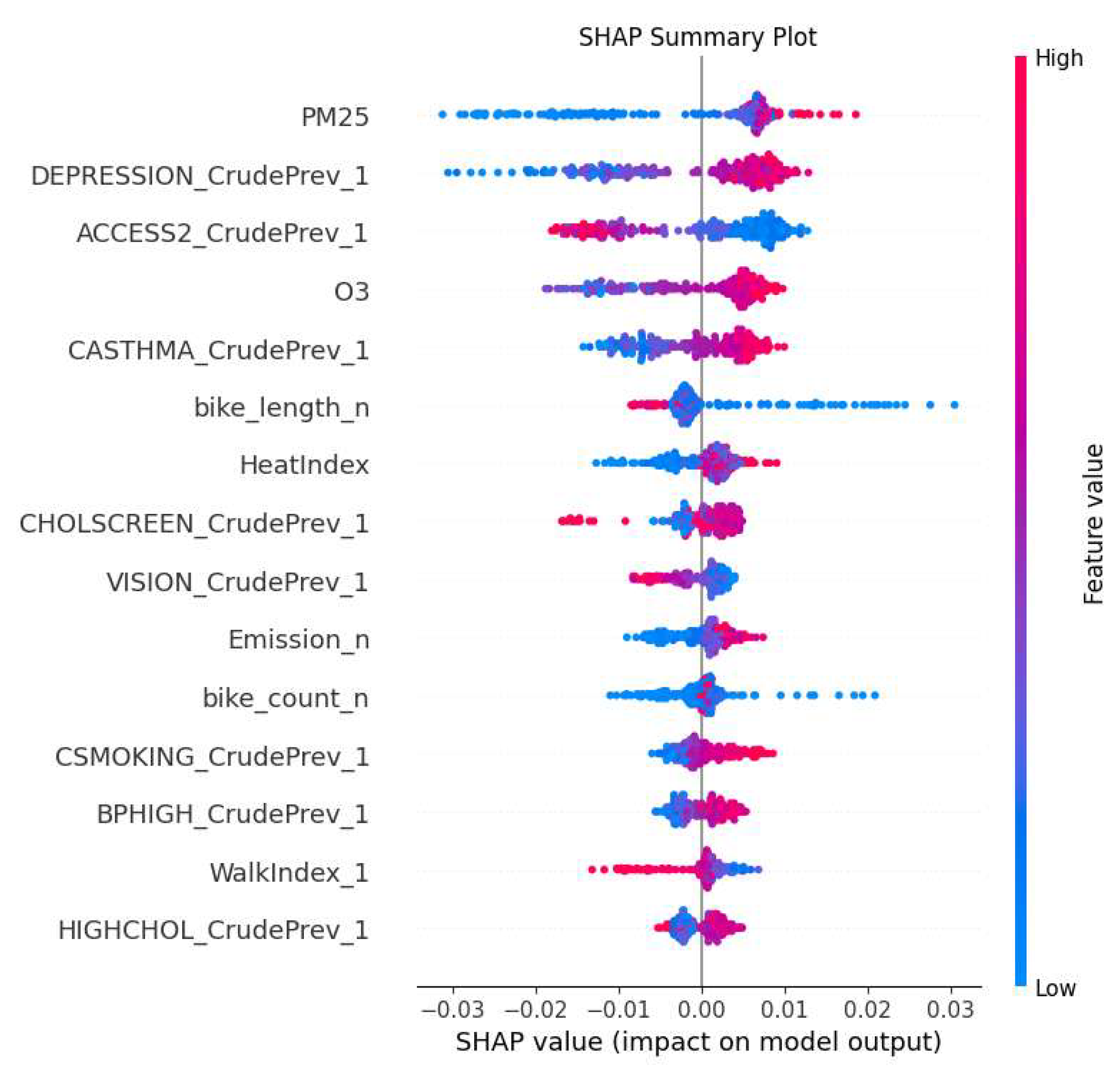
Figure 3.
Feature importance for Random Forest models on all types of cancers.
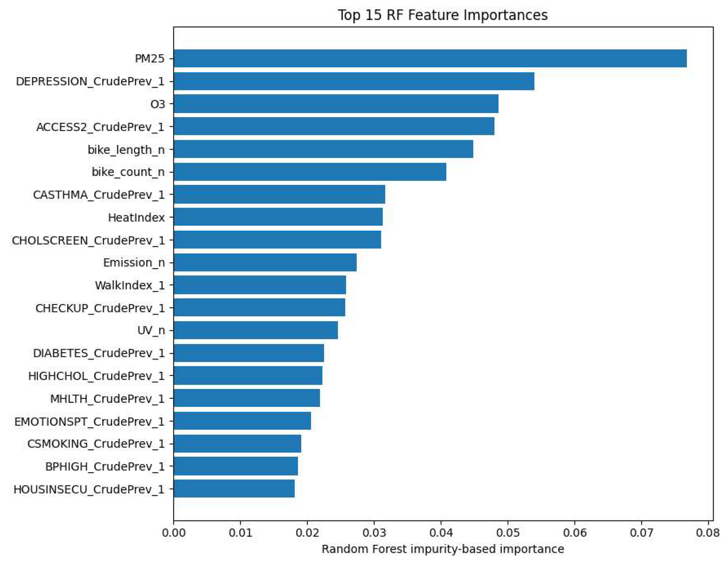
Figure 4.
The illustration of R2 value of all cancer types, skin cancer, colon cancer, and breast cancer analysis results.
Figure 4.
The illustration of R2 value of all cancer types, skin cancer, colon cancer, and breast cancer analysis results.
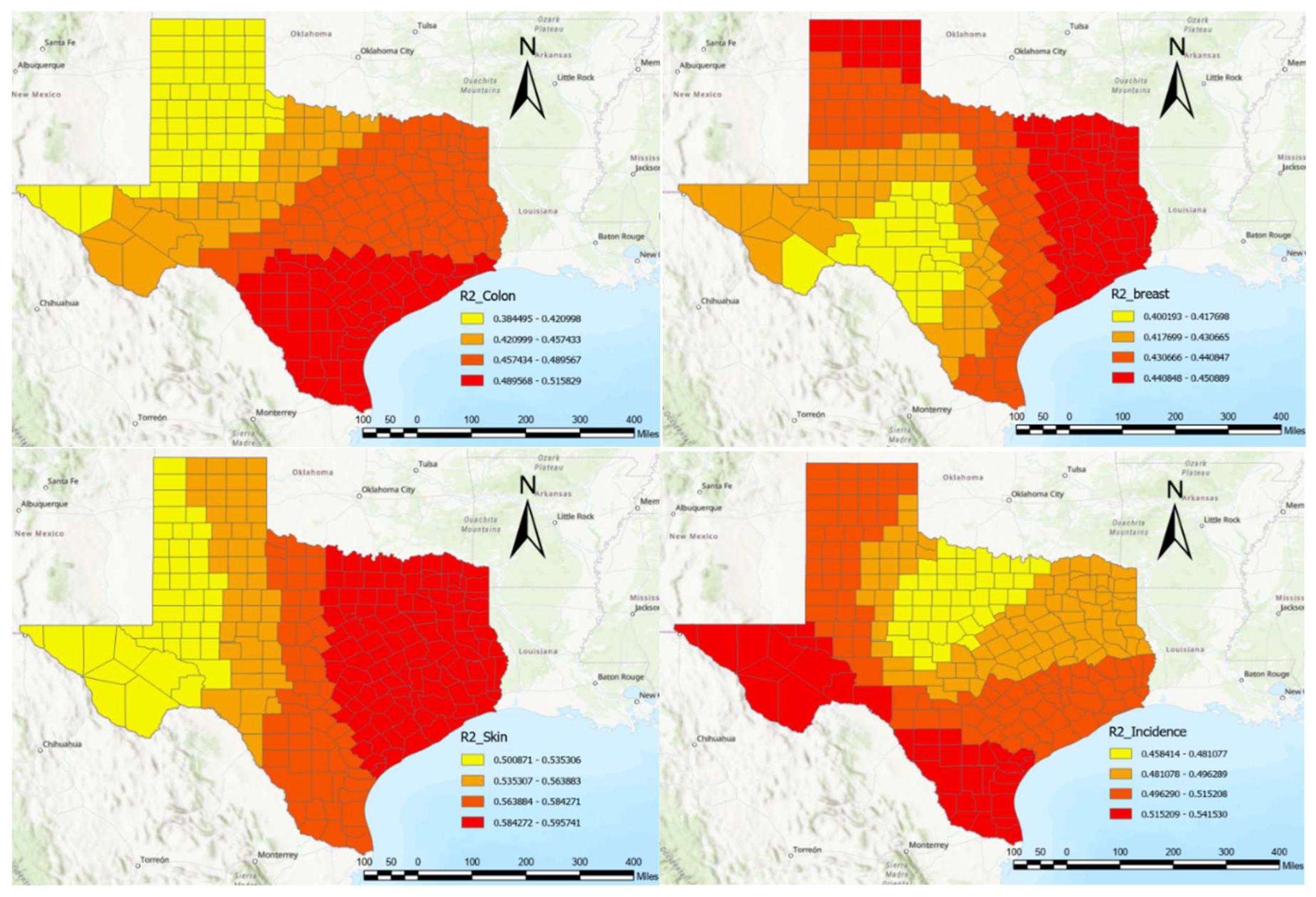
Figure 5.
The illustration of correlation coefficient value of No Leisure Time Activity variable to Colon Cancer incidences.
Figure 5.
The illustration of correlation coefficient value of No Leisure Time Activity variable to Colon Cancer incidences.
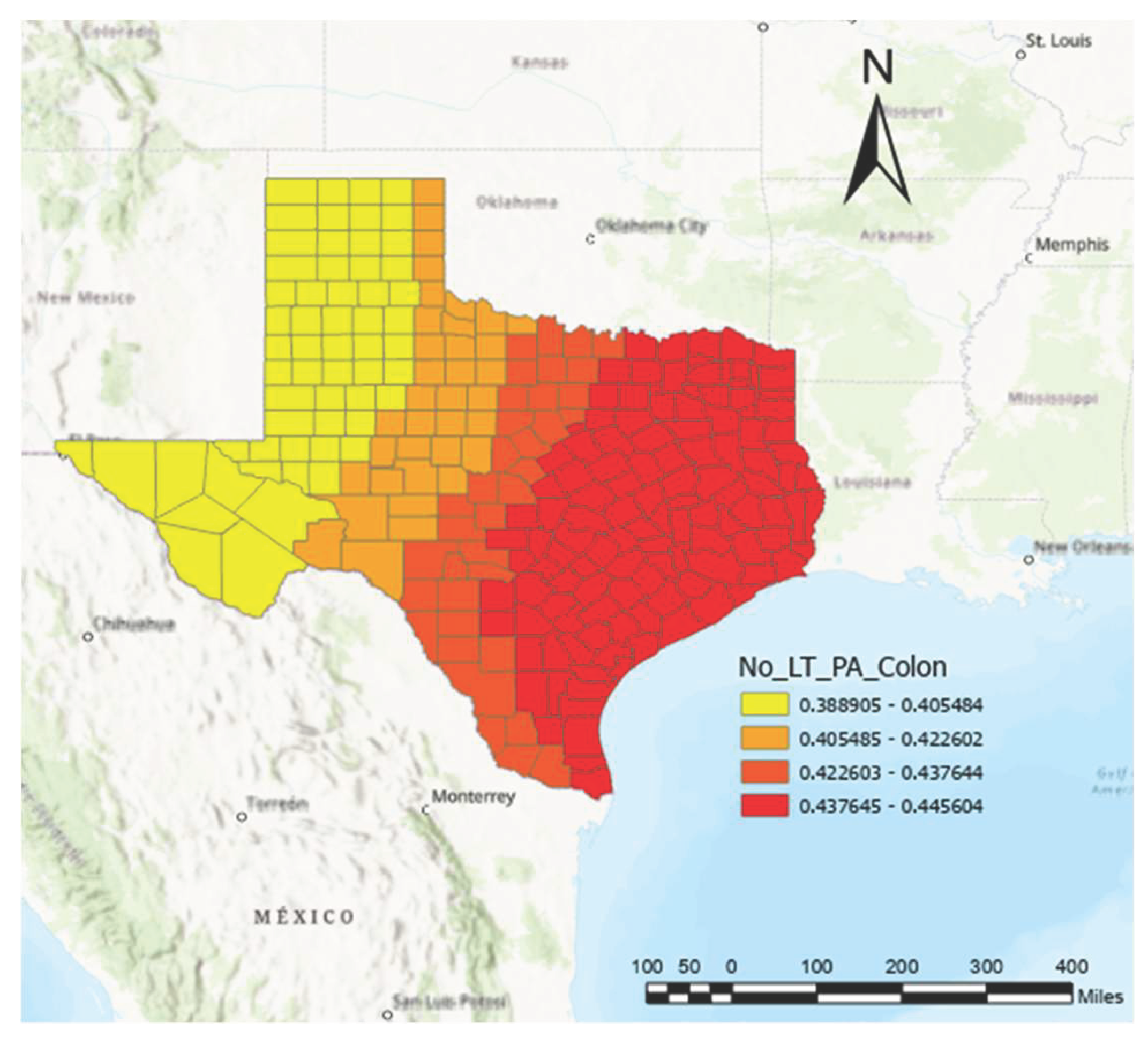
Table 1.
Attribute descriptions for variables used in the RF/SHAP and spatial regression analysis.
| Variable | Role | Base code | Description |
|---|---|---|---|
| ACCESS2_CrudePrev_1 | Predictor | ACCESS2 | County-level crude prevalence estimate for lack of health insurance among adults aged 18–64. |
| ARTHRITIS_CrudePrev_1 | Predictor | ARTHRITIS | County-level crude prevalence estimate for arthritis among adults. |
| BPHIGH_CrudePrev_1 | Predictor | BPHIGH | County-level crude prevalence estimate for adults ever told they had high blood pressure. |
| BPMED_CrudePrev_1 | Predictor | BPMED | County-level crude prevalence estimate for taking medication for high blood pressure among adults with hypertension. |
| CASTHMA_CrudePrev_1 | Predictor | CASTHMA | County-level crude prevalence estimate for current asthma among adults. |
| CHD_CrudePrev_1 | Predictor | CHD | County-level crude prevalence estimate for coronary heart disease among adults. |
| CHOLSCREEN_CrudePrev_1 | Predictor | CHOLSCREEN | County-level crude prevalence estimate for cholesterol screening among adults. |
| COPD_CrudePrev_1 | Predictor | COPD | County-level crude prevalence estimate for chronic obstructive pulmonary disease among adults. |
| OBESITY_CrudePrev_1 | Predictor | OBESITY | County-level crude prevalence estimate for obesity among adults. |
| GHLTH_CrudePrev_1 | Predictor | GHLTH | County-level crude prevalence estimate for fair or poor self-rated general health. |
| PHLTH_CrudePrev_1 | Predictor | PHLTH | County-level crude prevalence estimate for frequent physical distress. |
| DEPRESSION_CrudePrev_1 | Predictor | DEPRESSION | County-level crude prevalence estimate for adults ever diagnosed with depression. |
| CHECKUP_CrudePrev_1 | Predictor | CHECKUP | County-level crude prevalence estimate for having a routine medical checkup in the past year. |
| HIGHCHOL_CrudePrev_1 | Predictor | HIGHCHOL | County-level crude prevalence estimate for high cholesterol among screened adults. |
| DIABETES_CrudePrev_1 | Predictor | DIABETES | County-level crude prevalence estimate for diagnosed diabetes among adults. |
| STROKE_CrudePrev_1 | Predictor | STROKE | County-level crude prevalence estimate for adults ever diagnosed with stroke. |
| MHLTH_CrudePrev_1 | Predictor | MHLTH | County-level crude prevalence estimate for frequent mental distress. |
| SELFCARE_CrudePrev_1 | Predictor | SELFCARE | County-level crude prevalence estimate for self-care disability. |
| INDEPLIVE_CrudePrev_1 | Predictor | INDEPLIVE | County-level crude prevalence estimate for independent-living disability. |
| DISABILITY_CrudePrev_1 | Predictor | DISABILITY | County-level crude prevalence estimate for any disability. |
| VISION_CrudePrev_1 | Predictor | VISION | County-level crude prevalence estimate for vision disability. |
| COGNITION_CrudePrev_1 | Predictor | COGNITION | County-level crude prevalence estimate for cognitive disability. |
| SHUTUTILITY_CrudePrev_1 | Predictor | SHUTUTILITY | County-level crude prevalence estimate for risk of utility shutoff or utility insecurity. |
| LACKTRPT_CrudePrev_1 | Predictor | LACKTRPT | County-level crude prevalence estimate for lack of reliable transportation. |
| FOODINSECU_CrudePrev_1 | Predictor | FOODINSECU | County-level crude prevalence estimate for food insecurity. |
| HOUSINSECU_CrudePrev_1 | Predictor | HOUSINSECU | County-level crude prevalence estimate for housing insecurity. |
| EMOTIONSPT_CrudePrev_1 | Predictor | EMOTIONSPT | County-level crude prevalence estimate for lack of social and emotional support. |
| ISOLATION_CrudePrev_1 | Predictor | ISOLATION | County-level crude prevalence estimate for social isolation. |
| FOODSTAMP_CrudePrev_1 | Predictor | FOODSTAMP | County-level crude prevalence estimate for receiving SNAP or food stamp assistance. |
| Emission_n | Predictor | emission_n | Normalized county-level air-emission or pollution-related environmental indicator. |
| UV_n | Predictor | UV_n | Normalized county-level ultraviolet radiation exposure indicator. |
| Water_n | Predictor | Water_n | Normalized county-level water-related environmental indicator. |
| PM25 | Predictor | PM2.5 | County-level fine particulate matter exposure indicator used to represent air pollution. |
| O3 | Predictor | O3 | County-level ground-level ozone exposure indicator used to represent air pollution. |
| HeatIndex | Predictor | HeatIndex | County-level heat index indicator representing combined heat and humidity exposure. |
| bike_length_n | Predictor | Bike_length_n | Normalized county-level bicycle infrastructure or bicycle-network length indicator. |
| bike_count_n | Predictor | Bike_Count_n | Normalized county-level bicycle activity or bicycle-related feature count indicator. |
| WalkIndex_1 | Predictor | WalkIndex | County-level walkability index representing the relative walkability of the built environment. |
| No_LeisureTime_PA | Predictor | LPA | County-level proportion or prevalence of adults reporting no leisure-time physical activity. |
| Aerobic_PA | Predictor | Aerobic_PA | County-level proportion or prevalence of adults meeting aerobic physical activity recommendations. |
| CSMOKING_CrudePrev_1 | Predictor | CSMOKING | County-level crude prevalence estimate for current cigarette smoking among adults. |
| LPA_CrudePrev_1 | Predictor | LPA | County-level crude prevalence estimate for no leisure-time physical activity among adults. |
| ColorectalScreening | Predictor | COLON_SCREEN | County-level colorectal cancer screening prevalence or screening-compliance indicator. |
| DENTAL_CrudePrev_1 | Predictor | DENTAL | County-level crude prevalence estimate for visiting a dentist or dental clinic. |
| TEETHLOST_CrudePrev_1 | Predictor | TEETHLOST | County-level crude prevalence estimate for complete tooth loss among adults. |
| Incidence | Outcome | Incidence | Overall cancer incidence rate used as the all-site cancer outcome variable. |
| Age-Adjusted Rate_Breast_Normalized | Outcome | BreastCancer | Normalized age-adjusted breast cancer incidence rate. |
| Age-Adjusted Rate_Colon_Normalized | Outcome | ColonCancer | Normalized age-adjusted colon cancer incidence rate. |
| SkinCancer | Outcome | SkinCancer | Skin cancer incidence outcome variable used in the modeling analysis. |
| X_1 | Spatial coordinate | Longitude | County centroid longitude coordinate used for GWR and MGWR spatial modeling. |
| Y_1 | Spatial coordinate | Latitude | County centroid latitude coordinate used for GWR and MGWR spatial modeling. |
Disclaimer/Publisher’s Note: The statements, opinions and data contained in all publications are solely those of the individual author(s) and contributor(s) and not of MDPI and/or the editor(s). MDPI and/or the editor(s) disclaim responsibility for any injury to people or property resulting from any ideas, methods, instructions or products referred to in the content. |
© 2026 by the authors. Licensee MDPI, Basel, Switzerland. This article is an open access article distributed under the terms and conditions of the Creative Commons Attribution (CC BY) license (http://creativecommons.org/licenses/by/4.0/).
Copyright: This open access article is published under a Creative Commons CC BY 4.0 license, which permit the free download, distribution, and reuse, provided that the author and preprint are cited in any reuse.