

Submitted:
13 July 2026
Posted:
14 July 2026
You are already at the latest version
Abstract
The demand for user-friendly applications to support biologists in analyzing high-throughput proteomics data remains a pressing challenge. Given the complexity and the multiple intermediate steps involved, this process is time-consuming and often requires specialized computational skills. To simplify and accelerate the exploration of proteomics data, we present PiProteline, an R package designed to operate on high-dimensional data matrices assembled from the output of any search engine commonly used in bottom-up proteomics experiments. In addition to data preprocessing and descriptive statistics, PiProteline enables label-free quantitation, functional enrichment, and systems biology analyses. Notably, it supports both unweighted and weighted protein-protein interaction (PPI) network topological analyses for the identification of critical nodes, such as hubs and bottlenecks. By integrating multiple analytical approaches, PiProteline accelerates the selection of potentially relevant protein signatures, providing insights into the molecular mechanisms characterizing the investigated systems. This information facilitates the formulation of new hypotheses and the design of targeted experiments, ultimately reducing costs and advancing translational medicine. PiProteline is available as an open-source R package via GitHub (https://github.com/lomi95/PiProteline) and as a Shiny application (https://github.com/salehnhd/PiProteline-Shiny).
Keywords:
proteomics
; bioinformatics
; systems biology
; R package
1. Introduction
The study of biological systems through multiomic profiling has become an increasingly prevalent approach in modern biology [1].This strategy serves a dual purpose: it aims to elucidate the molecular mechanisms underlying the phenotypes and genotypes under investigation, while also functioning as a preliminary screening tool for the discovery of potential biomarkers or key regulatory molecules. Since proteins are the primary effectors of most biological functions, their comprehensive investigation is essential to achieving these goals and, consequently, to advancing precision medicine [2]. The foundation for this pursuit was laid by whole-genome sequencing, which catalyzed the development of high-throughput proteomic technologies based on mass spectrometry (MS) and liquid chromatography (LC)—milestones that have profoundly shaped the field [3]. Consequently, it is now possible to analyze the protein composition of complex biological samples—including cell lines and tissues—with remarkable speed, accuracy, and reproducibility, while maintaining high sensitivity and relatively low cost. Furthermore, recent methodological innovations, such as Data Independent Acquisition (DIA), have enabled increasingly deep proteomic coverage, allowing the qualitative and quantitative characterization of several thousand proteins per sample or analytical run [4].
In addition to the analytical phase, a typical proteomics pipeline workflow comprises several computational steps, including raw spectra interpretation, data preprocessing, protein quantitation, and functional evaluation [5]. Regarding raw spectra interpretation, both commercial and free-of-charge software are available [6]. Many of these tools are already integrated with utilities that provide a comprehensive package of results, including protein profiles, differentially expressed proteins, and enriched Gene Ontology (GO) terms and biological pathways. However, the variety of MS search engine algorithms, formats, statistics, and data filtering approaches makes post-protein identification data analysis challenging. Consequently, the evaluation of the same raw data through different computational pipelines can yield divergent results [7].
To simplify proteomics data exploration across multiple platforms and create tools that can be assembled into logical, customizable, and reproducible workflows, several R packages addressing specific needs have been released, including those for protein quantitation [8,9,10], statistical analysis [11], and functional assessment of multiomics data [12]. Packages that integrate all these functions, providing a more comprehensive set of results, have also been proposed [13,14].
Although the scientific community is actively addressing these challenges, the need for easy-to-use applications to support biologists in synthesizing proteomic data remains current. Indeed, this workflow, which involves multiple analysis steps, is time-consuming and often requires specific IT skills. To facilitate these activities, we present PiProteline. Developed as an R package and Shiny application, it operates on high-dimensional data matrices assembled from the output of any search engine software commonly used in bottom-up proteomics experiments. In addition to data preprocessing, such as cleaning and normalization, PiProteline enables descriptive statistics, differential expression analysis, and functional enrichment, accompanied by result visualization. Notably, it also supports both weighted and unweighted network analyses with automated selection of the corresponding hubs and bottlenecks [15,16].
2. Materials and Methods
2.1. PiProteline R Code
PiProteline runs on all major operating systems, and the released version is available via GitHub as an open-source R package (https://github.com/lomi95/PiProteline); the data used for testing PiProteline, and the corresponding outputs, including tables and graphs, are available. Full documentation is provided within the README.md files. For PiProteline R package development, key libraries include tidyverse for data manipulation and visualization [17], rbioapi for functional enrichment [18], and igraph v2.1.4 for graph analysis [19].
2.2. Shiny APP
A Shiny web application (https://github.com/salehnhd/PiProteline-Shiny) integrating PiProteline’s functionality was developed using RStudio v2025.9.0.387. The interface was built using shiny v1.11.1 [20], shinyWidgets v0.9.0 [21], DT v0.34.0 [22], and ggplot2 v3.5.2 [23].
2.3. Data Test
To test PiProteline’s functionality, we used a set of proteomic profiles obtained from the analysis of substantia nigra samples from healthy controls (C, n = 20), patients with Parkinson’s disease (PD, n = 20), and patients with Parkinson’s disease carrying a GBA1 mutation [24]. Specifically, spectral counts (SpCs) per identified protein were used as the quantitative parameter.
3. Results
3.1. PiProteline Workflow
PiProteline supports the output of any search engine software commonly used in bottom-up proteomics experiments, including MaxQuant, Proteome Discoverer, Spectrum Mill, and Skyline [6]. It works with data obtained from both data-dependent acquisition (DDA) and data-independent acquisition (DIA), adequately formatted as a high-dimensional data matrix m x n (Figure 1). The main PiProteline steps include data pre-processing, label-free differential expression, functional enrichment and network analysis (Figure 2). Compared to other similar R packages, network analysis represents a novel feature. In particular, it enables both unweighted and weighted network topological analyses with automated selection of critical nodes, such as hubs and bottlenecks [15], which are combined with differential expression analysis for the selection of the most putatively relevant proteins [16].
3.1.1. Pre-Processing
In a proteomics data matrix obtained by processing MS raw data through search engine software and a FASTA database, it is common to find protein isoforms corresponding to the same gene name. Since we refer to the gene name as the primary key for building protein-protein interaction (PPI) network models, PiProteline eliminates these redundant entries by retaining the maximum value (AU, i.e., SpC/Intensity/Peak Area) per sample (Figure 3A). After removing redundancies, the data may be normalized using different strategies, including total signal normalization, Z-score normalization, maximum signal normalization, row sigma normalization, unit vector normalization, min-max normalization, and logarithmic transformation [25], (Figure 3B). Finally, the data are filtered based on protein identification frequency (IF). A first dataset, referred to as datafull, contains all proteins. A second dataset, referred to as data100%, extracts for each group/condition only proteins found in all samples (IF=100% per group/condition). Finally, a dataset termed datashared is created by considering only proteins found in all samples across all conditions (IF=100% in all groups/conditions). These datasets are processed in subsequent steps. For convenience, we refer to lists of datasets rather than individual datasets, since filters are applied according to the studied conditions or groups (Figure 3C).
Before proceeding to the next steps, PiProteline performs exploratory data analysis to assess missing values, as well as the mean, minimum, and maximum protein abundances within the dataset, and the mean and standard deviation values for individual samples. Moreover, Spearman’s correlation between groups is calculated using the entire protein dataset.
3.1.2. Quantitative Analysis
PiProteline’s protein quantitation is based on a label-free strategy that exploits spectral counts (SpC), peak area, or intensity as quantitative parameters. When the data matrix contains more than six replicates per condition, multivariate ANOVA (MANOVA) and Benjamini-Hochberg correction are applied [26]. Differentially expressed proteins (DEPs) are extracted by processing the complete normalized data matrix (datafull), which is used both for comparing all groups simultaneously (when more than two groups/conditions are available) and in pairwise comparisons. In any case, fold change and Differential Average (DAve) index are calculated to establish the expression trend in pairwise comparisons [5].
Once DEPs are extracted, they serve as input for the Random Forest model [27], which calculates the distance between the groups/conditions analyzed. This distance allows reconstruction of a multidimensional scaling (MDS) plot, reducing the original dataset’s dimensionality and visually displaying the separation between groups/conditions and the amount of variance explained (Figure 4).
The features (DEPs) extracted are also used to build a volcano plot, where the x-axis represents the fold change (FC) and the y-axis displays . Both parameters can be filtered by setting appropriate thresholds (e.g., and ) to select DEPs with the desired level of significance (Figure 5).
Furthermore, protein expression variation in pairwise comparisons is evaluated through the DAve index, which is incorporated into the output files alongside other statistical parameters.
Specifically, fold change (FC) is defined as:
where is a default pseudocount ().
While, the Differential Average (DAve) index is defined as:
where and represent the quantitative parameter (expressed as arbitrary unit, AU, i.e., spectral count, peak area or intensity) of a given protein in two compared groups/conditions (X and Y). By convention, the DAve sign (+/-) indicates the expression trend, with positive DAve denoting proteins up-regulated in the first group/condition (X) and negative DAve denoting proteins up-regulated in the second group/condition (Y) [5].
3.2. Network Analysis
PiProteline enables network topological analysis through two different strategies: Unweighted Network Analysis (UNA) and Weighted Network Analysis (WNA). However, to obtain reliable results, it is not recommended to rely on WNA if fewer than 20–30 samples/profiles per group/condition are available [28]. By default, UNA takes as input the data100% dataset, which consists of proteins found in all samples of a given group/condition (IF=100%). Notably, the identification frequency (IF) threshold can be modified to consider a wider set of proteins. In contrast, WNA uses the datashared dataset, which includes proteins identified in all samples across all groups. In this case, the IF cannot be changed because WNA requires a data matrix without missing values.
For both UNA and WNA, protein-protein interactions (PPIs) models are reconstructed starting from STRING-db [29]. For UNA, an undirected and unweighted graph is reconstructed, while for WNA, an undirected graph is generated and subsequently weighted using a modified Spearman’s correlation score [16] calculated from the experimental data matrix (datashared).
After PPI graph reconstruction, the largest connected component is extracted and analyzed topologically. Disconnected or isolated nodes are removed. Centrality measures, including betweenness, centroid, and bridging, are calculated to identify critical nodes, such as hubs and bottlenecks [15,16]. Specifically, they are defined as:
- Hubs: Nodes with betweenness and centroid values greater than the 75th percentile.
- Bottlenecks: Nodes with betweenness and bridging values greater than the 75th percentile.
Hubs and bottlenecks are further classified into three categories (Table 1):
- NotSpecific: Nodes whose centralities meet the 75th percentile criteria in any group/condition.
- Specific: Nodes whose centralities meet the 75th percentile criteria in a group/condition but not in all others.
- Centrality Specific: Nodes whose centralities satisfy the 75th percentile criterion in one group/condition, while in all others no centralities exceed the threshold.
3.3. Functional Analysis
Functional enrichment analysis is performed using Gene Ontology (GO) terms and pathways from Reactome, KEGG, and WikiPathways databases as references. A single-profile enrichment considers the proteins found in each individual sample. Following the processing of all samples, a t x s data matrix is generated, where t represents the enriched term and s represents the sample in which it was enriched.The generic element reports the number of proteins in the j-th sample that allowed the enrichment of the i-th term. MANOVA is then applied to select GO terms and pathways that are differentially enriched among the considered groups/conditions (Figure 6A).
Functional enrichment is also performed using DEPs from quantitative analysis, and hubs and bottlenecks from network analysis. For protein quantitation, enrichment is conducted on DEPs extracted from each pairwise comparison. To simplify the output, PiProteline provides a table with exclusive differentially enriched terms (e.g., if a term is enriched from both up- and down-regulated proteins in X vs Y comparison, it is removed from the output) (Figure 6B).
Enrichment analysis is finally carried out using topologically relevant proteins extracted from network analysis. The enrichment is evaluated for both UNA and WNA outputs, as well as for each group/condition under study. As for DEPs, to provide group-specific information, pairwise comparisons are performed and an output table reporting exclusive terms is created.
To integrate quantitative and network analyses, the terms enriched in both steps are compared for each pairwise comparison. A list is generated distinguishing terms with consistent trends (e.g., in the X vs Y comparison, terms identified exclusively in X vs Y) and terms with opposing trend (e.g., terms enriched in X based on quantitative analysis but enriched in Y based on network analysis, or vice versa).
3.4. Summary Tables
To summarize the volume of information generated by PiProteline, different output tables are provided. They include:
- output_unfiltered_results: Contains all unfiltered results (i.e., Quantitative Analysis (all vs all), Quantitative Analysis (pairwise comparisons), UNA, WNA, Summary).
- output_significative_results: Contains all results filtered based on the thresholds set (i.e., Quantitative Analysis (all vs all), Quantitative Analysis (pairwise comparisons), UNA (NotSpecific, Specific, CentralitySpecific), WNA (NotSpecific, Specific, CentralitySpecific).
- output_enrichment: Includes single profile enrichment and enrichment from quantitative and network topology pairwise comparisons.
- output_enrichmentTrend: Includes tables reporting GO terms and pathways with the same or opposing trends from quantitative and network analysis.
The Summary table, included in the output_unfiltered_results file, encompasses all data processing steps. Notably, it also includes two additional columns:
- Total Significance Count: The number of analyses in which a given protein was found to be significant.
- Weighted Significance Score: A weighted score normalized based on the type of analysis in which a given protein was found to be significant.
The score is calculated as follows:
where:
- M = number of times a given protein was significant in pairwise quantitative comparisons (MANOVA)
- w = number of times a given protein was significant by WNA
- s = number of times a given protein was a “specific” critical node
- = number of times a given protein was a “centrality-specific” critical node
By sorting the Summary table by total significance count or weighted significance score, proteins that were found to be significant across multiple analyses can be quickly identified. Thus, this score provides an immediate overview of proteins that potentially represent promising targets for further investigation and targeted experiments.
4. Discussion and Conclusions
The PiProteline R package presented here aims to expedite a computational pipeline for comprehensive evaluation of high-throughput proteomics results following protein identification. It offers the advantage of automating complex and repetitive analyses, reducing human error, and improving overall workflow efficiency. In addition to streamlining these steps, PiProteline contributes to increased standardization, facilitating the comparison of results obtained from different studies, as well as from different analytical instruments and search engine software. Indeed, the intrinsic heterogeneity of proteomic workflows, arising from the combination of multiple analytical and computational tools, exacerbates the low reproducibility of results obtained even from the same raw data [7].
Overall, PiProteline is intended as a flexible and integrative tool for exploratory and comparative proteomic analysis. As an increasing number of studies rely on high-throughput proteomic data, and the volume of data produced continues to grow, the availability of tools that simplify and standardize data processing represents a competitive advantage, freeing up valuable time for subsequent investigations and facilitating future clinical applications [31]. For this purpose, we emphasize that, in addition to quantitative and functional analysis, PiProteline is the only tool that integrates weighted and unweighted network topology for the selection of hubs and bottlenecks [15,16]. This information, integrated with traditional quantitative analysis, represents a fundamental step in filtering the most potentially interesting molecules, thereby accelerating the discovery of markers through targeted experiments that reduce unnecessary costs and facilitate translational medicine [32].
PiProteline’s modularity and flexibility allow users to tailor each step to the specific characteristics of their dataset and objectives. In this regard, we note that, since PiProteline operates on a high-dimensional data matrix assembled from the output of any search engine software commonly used in bottom-up proteomics experiments, its potential applications are very broad [33]. Furthermore, the development of a Shiny application aims to facilitate and promote the use of PiProteline even for users without advanced bioinformatics skills and/or those primarily dedicated to other fundamental steps of the proteomic workflow, such as sample preparation or management of the analytical-instrumental phase.
From the perspective of future developments, the R environment facilitates the integration of new features, such as the implementation of existing steps or the addition of new ones customized for specific data types, including transcriptomics and metabolomics. These improvements could include new statistical models for quantitative analysis (both labeled and label-free), the use of signaling networks, and strategies for multiomics data integration [34]. Additionally, functional improvements to the Shiny application, including results visualization and sharing on a web server, will represent further steps towards making PiProteline increasingly easy to use for an even wider segment of the scientific community dedicated to the analysis of omics data.
Author Contributions
Conceptualization, A.L. and D.DS.; methodology, A.L., S.H., I.Y.; software, A.L. and S.H.; formal analysis, A.L., S.H., I.Y.; resources, PL.M. and D.DS; data curation, A.L. and S.H.; writing—original draft preparation, A.L., S.H., I.Y., PL.M and D.DS.; writing—review and editing, A.L., D.DS.; supervision, D.DS.; funding acquisition, PL.M. and D.DS. All authors have read and agreed to the published version of the manuscript.
Funding
This research was funded by Italian Ministry of University and Research (PRIN2022: 2022Z2TE5P (DDS) and PRIN2022: 2022LNHZAP (PLM)).
Institutional Review Board Statement
Not applicable.
Informed Consent Statement
Not applicable.
Data Availability Statement
The data used to generate the results are available (https://github.com/lomi95/PiProteline). The original dataset is publicly available from the study “Large-scale proteomics analysis of five brain regions from Parkinson’s disease patients with a GBA1 mutation” (DOI: https://doi.org/10.1038/s41531-024-00645-x). The PiProteline R package is available on GitHub (https://github.com/lomi95/PiProteline), as well as the corresponding Shiny web application (https://github.com/salehnhd/PiProteline-Shiny.
Acknowledgments
The authors thank the Italian node of the ELIXIR infrastructure, coordinated by the National Research Council (CNR) (ELIXIRxNextGenIT, PNRR, Prot.IR0000010)
Conflicts of Interest
The authors declare no conflicts of interest. The funders had no role in the design of the study; in the collection, analyses, or interpretation of data; in the writing of the manuscript; or in the decision to publish the results.
Abbreviations
The following abbreviations are used in this manuscript:
| AU | Arbitrary Unit |
| BP | Biological Process |
| C | Control |
| DAve | Differential Average |
| DDA | Data-Dependent Acquisition |
| DEP | Differentially Expressed Protein |
| DIA | Data-Independent Acquisition |
| FC | Fold Change |
| FDR | False Discovery Rate |
| GO | Gene Ontology |
| IF | Identification Frequency |
| KEGG | Kyoto Encyclopedia of Genes and Genomes |
| LC | Liquid Chromatography |
| MANOVA | Multivariate Analysis of Variance |
| MDS | Multidimensional Scaling |
| MS | Mass Spectrometry |
| PD | Parkinson’s Disease |
| PG | Parkinson’s Disease with GBA1 Mutation |
| PPI | Protein-Protein Interaction |
| SpC | Spectral Count |
| UNA | Unweighted Network Analysis |
| WNA | Weighted Network Analysis |
References
- Babu, M.; Snyder, M. Multi-Omics Profiling for Health. Molecular &Cellular Proteomics 2023, 22, 100561. [CrossRef]
- Jiang, Y.; Wang, J.; Sun, A.; Zhang, H.; Yu, X.; Qin, W.; Ying, W.; Li, Y.; Chang, C.; Wang, X.; et al. The coming era of proteomics-driven precision medicine. National Science Review 2025, 12. [CrossRef]
- Nilsson, T.; Mann, M.; Aebersold, R.; Yates, J.R.; Bairoch, A.; Bergeron, J.J. Mass spectrometry in high-throughput proteomics: Ready for the big time. Nature Methods 2010, 7, 681–685. [CrossRef]
- Mun, D.G.; Renuse, S.; Saraswat, M.; Madugundu, A.; Udainiya, S.; Kim, H.; Park, S.K.R.; Zhao, H.; Nirujogi, R.S.; Na, C.H.; et al. PASS-DIA: A Data-Independent Acquisition Approach for Discovery Studies. Analytical chemistry 2020, 92, 14466–14475. [CrossRef]
- Dario DiSilvestre, Francesca Brambilla, G.M.; Mauri, P. Computational Tools and Methods for the Study of Systemic Amyloidosis at the Clinical and Molecular Level. Methods in molecular biology (Clifton, N.J.) 2025, 2884, 369–387. [CrossRef]
- Halder, A.; Verma, A.; Biswas, D.; Srivastava, S. Recent advances in mass-spectrometry based proteomics software, tools and databases. Drug Discovery Today: Technologies 2021, 39, 69–79. [CrossRef]
- Bouyssié, D.; Altıner, P.; Capella-Gutierrez, S.; Fernández, J.M.; Hagemeijer, Y.P.; Horvatovich, P.; Hubálek, M.; Levander, F.; Mauri, P.; Palmblad, M.; et al. WOMBAT-P: Benchmarking Label-Free Proteomics Data Analysis Workflows. Journal of proteome research 2024, 23, 418–429. [CrossRef]
- Rosenberger, G.; Ludwig, C.; Röst, H.L.; Aebersold, R.; Malmström, L. aLFQ: an R-package for estimating absolute protein quantities from label-free LC-MS/MS proteomics data. Bioinformatics (Oxford, England) 2014, 30, 2511–2513. [CrossRef]
- Wolski, W.E.; Nanni, P.; Grossmann, J.; d’Errico, M.; Schlapbach, R.; Panse, C. prolfqua: A Comprehensive R-Package for Proteomics Differential Expression Analysis. Journal of proteome research 2023, 22, 1092–1104. [CrossRef]
- Ranathunge, C.; Patel, S.S.; Pinky, L.; Correll, V.L.; Chen, S.; Semmes, O.J.; Armstrong, R.K.; Combs, C.D.; Nyalwidhe, J.O. promor: a comprehensive R package for label-free proteomics data analysis and predictive modeling. Bioinformatics advances 2023, 3. [CrossRef]
- Welham, Z.; Déjean, S.; Cao, K.A.L. Multivariate Analysis with the R Package mixOmics. Methods in molecular biology (Clifton, N.J.) 2023, 2426, 333–359. [CrossRef]
- Danna, V.; Mitchell, H.; Anderson, L.; Godinez, I.; Gosline, S.J.; Teeguarden, J.; McDermott, J.E. leapR: An R Package for Multiomic Pathway Analysis. Journal of proteome research 2021, 20, 2116–2121. [CrossRef]
- Jones, J.; MacKrell, E.J.; Wang, T.Y.; Lomenick, B.; Roukes, M.L.; Chou, T.F. Tidyproteomics: an open-source R package and data object for quantitative proteomics post analysis and visualization. BMC Bioinformatics 2023, 24, 1–14. [CrossRef]
- Quast, J.P.; Schuster, D.; Picotti, P. protti: an R package for comprehensive data analysis of peptide- and protein-centric bottom-up proteomics data. Bioinformatics Advances 2022, 2. [CrossRef]
- Vella, D.; Zoppis, I.; Mauri, G.; Mauri, P.; Silvestre, D.D. From protein-protein interactions to protein co-expression networks: a new perspective to evaluate large-scale proteomic data. Eurasip Journal on Bioinformatics and Systems Biology 2017, 2017, 1–16. [CrossRef]
- Lomagno, A.; Yusuf, I.; Tosadori, G.; Bonanomi, D.; Mauri, P.L.; Silvestre, D.D. CoPPIs algorithm: a tool to unravel protein cooperative strategies in pathophysiological conditions. Briefings in bioinformatics 2025, 26. [CrossRef]
- Wickham, H. Easily Install and Load the ’Tidyverse’ [R package tidyverse version 2.0.0]. CRAN: Contributed Packages 2023. [CrossRef]
- Rezwani, M. User-Friendly R Interface to Biologic Web Services’ API [R package rbioapi version 0.8.2]. CRAN: Contributed Packages 2025. [CrossRef]
- Csárdi, G.; Nepusz, T.; Müller, K.; Horvát, S.; Traag, V.; Zanini, F.; Noom, D. igraph for R: R interface of the igraph library for graph theory and network analysis, 2026. [CrossRef]
- Chang, W.; Cheng, J.; Allaire, J.; Sievert, C.; Schloerke, B.; Xie, Y.; Allen, J.; McPherson, J.; Dipert, A.; Borges, B. Web Application Framework for R [R package shiny version 1.11.1]. CRAN: Contributed Packages 2025. [CrossRef]
- Perrier, V.; Meyer, F.; Granjon, D. Custom Inputs Widgets for Shiny [R package shinyWidgets version 0.9.0]. CRAN: Contributed Packages 2025. [CrossRef]
- Xie, Y.; Cheng, J.; Tan, X.; Aden-Buie, G. A Wrapper of the JavaScript Library ’DataTables’ [R package DT version 0.34.0]. CRAN: Contributed Packages 2025. [CrossRef]
- Wickham, H.; Chang, W.; Henry, L.; Pedersen, T.L.; Takahashi, K.; Wilke, C.; Woo, K.; Yutani, H.; Dunnington, D.; van den Brand, T. Create Elegant Data Visualisations Using the Grammar of Graphics [R package ggplot2 version 4.0.0]. CRAN: Contributed Packages 2025. [CrossRef]
- Blumenreich, S.; Nehushtan, T.; Kupervaser, M.; Shalit, T.; Gabashvili, A.; Joseph, T.; Milenkovic, I.; Hardy, J.; Futerman, A.H. Large-scale proteomics analysis of five brain regions from Parkinson’s disease patients with a GBA1 mutation. NPJ Parkinson’s Disease 2024, 10, 33. [CrossRef]
- Carvalho, P.C.; Hewel, J.; Barbosa, V.C.; Yates, J.R. Identifying differences in protein expression levels by spectral counting and feature selection. Genetics and molecular research : GMR 2008, 7, 342–356. [CrossRef]
- Buderer, N.M.; Brannan, G.D. Comparing the Means of Independent Groups: ANOVA, ANCOVA, MANOVA, and MANCOVA. StatPearls 2024.
- Hu, J.; Szymczak, S. A review on longitudinal data analysis with random forest. Briefings in Bioinformatics 2023, 24, 1–11. [CrossRef]
- Jack R. Fraenkel, Norman E. Wallen, H.H.R.P. How to design and evaluate research in education; McGraw-Hill Humanities/Social Sciences/Languages, 2011.
- Szklarczyk, D.; Nastou, K.; Koutrouli, M.; Kirsch, R.; Mehryary, F.; Hachilif, R.; Hu, D.; Peluso, M.E.; Huang, Q.; Fang, T.; et al. The STRING database in 2025: protein networks with directionality of regulation. Nucleic acids research 2025, 53, D730–D737. [CrossRef]
- Zhu, W.; Smith, J.W.; Huang, C.M. Mass spectrometry-based label-free quantitative proteomics. Journal of biomedicine & biotechnology 2010, 2010. [CrossRef]
- Guo, T.; Steen, J.A.; Mann, M. Mass-spectrometry-based proteomics: from single cells to clinical applications. Nature 2025 638:8052 2025, 638, 901–911. [CrossRef]
- and Alonso-Andrés, P.; Baldazzi, D.; Chen, Q.; Conde Moreno, E.; Crespo-Toro, L.; Donner, K.; Džubák, P.; Ekberg, S.; García Bermejo, M.L.; Gasparotto, D.; et al. Multi-omics Quality Assessment in Personalized Medicine Through European Infrastructure for Translational Medicine (EATRIS): An Overview. Phenomics 2025, 5, 311–325. [CrossRef]
- Vincent, A.T.; Charette, S.J. Who qualifies to be a bioinformatician? Frontiers in Genetics 2015, 6, 134173. [CrossRef]
- Dexter, A.; Thomas, S.A.; Steven, R.T.; Robinson, K.N.; Taylor, A.J.; Elia, E.A.; Nikula, C.; Campbell, A.D.; Panina, Y.; Najumudeen, A.K.; et al. A New Approach to Large Multiomics Data Integration. Analytical Chemistry 2025, 97, 20058–20067. [CrossRef]
Figure 1.
Overview of PiProteline input data structure. PiProteline accepts high-dimensional data matrices formatted as m x n where, rows m represent proteins and columns n represent individual samples. The input can be derived from the output of any search engine software commonly used in bottom-up proteomics experiments (e.g., MaxQuant, Proteome Discoverer, Spectrum Mill, Skyline) and supports data obtained from both data-dependent acquisition (DDA) and data-independent acquisition (DIA). The matrix contains quantitative values expressed as arbitrary units (AU), such as spectral counts (SpC), peak area, or intensity, depending on the quantification method employed [30].
Figure 1.
Overview of PiProteline input data structure. PiProteline accepts high-dimensional data matrices formatted as m x n where, rows m represent proteins and columns n represent individual samples. The input can be derived from the output of any search engine software commonly used in bottom-up proteomics experiments (e.g., MaxQuant, Proteome Discoverer, Spectrum Mill, Skyline) and supports data obtained from both data-dependent acquisition (DDA) and data-independent acquisition (DIA). The matrix contains quantitative values expressed as arbitrary units (AU), such as spectral counts (SpC), peak area, or intensity, depending on the quantification method employed [30].
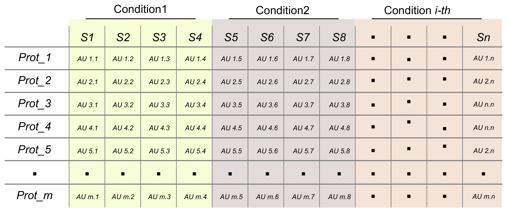
Figure 2.
PiProteline workflow flowchart. Diagram summarizing the main steps of PiProteline R package. These include data preprocessing, descriptive statistics, quantitative analysis, network analysis, and functional enrichment analysis. Differentially expressed proteins (DEPs) and topologically relevant nodes, such as hubs and bottlenecks, represent intermediate outputs that feed into subsequent analytical steps.
Figure 2.
PiProteline workflow flowchart. Diagram summarizing the main steps of PiProteline R package. These include data preprocessing, descriptive statistics, quantitative analysis, network analysis, and functional enrichment analysis. Differentially expressed proteins (DEPs) and topologically relevant nodes, such as hubs and bottlenecks, represent intermediate outputs that feed into subsequent analytical steps.
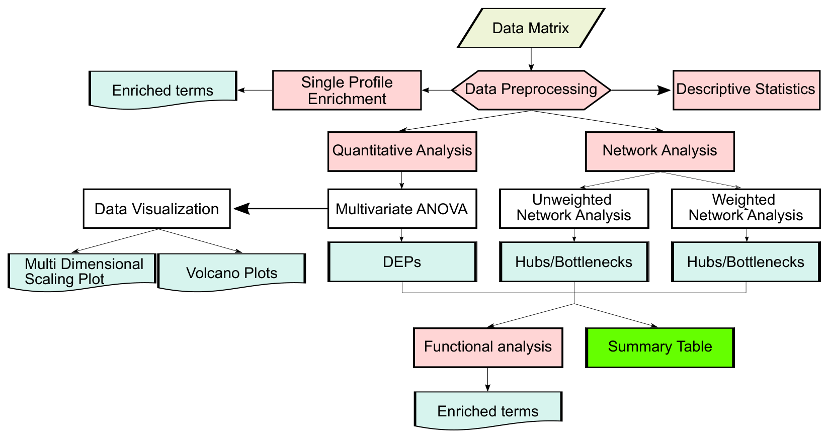
Figure 3.
Data preprocessing workflow. A) The original data matrix is processed to remove duplicate entries corresponding to protein isoforms by retaining the maximum abundance value per sample. B) Data normalization is performed using various strategies; total signal normalization is shown as an example, which transforms the data so that each sample (column) exhibits an equal sum of spectral counts (SpCs), intensity, or peak area. C) Three intermediate datasets, datafull, data100% and datashared, are generated based on identification frequency (IF) thresholds. datafull contains all identified proteins; data100% includes only proteins found in all samples within each group/condition (IF = 100% per group); and datashared comprises proteins identified in all samples across all experimental conditions (IF = 100% across all groups).
Figure 3.
Data preprocessing workflow. A) The original data matrix is processed to remove duplicate entries corresponding to protein isoforms by retaining the maximum abundance value per sample. B) Data normalization is performed using various strategies; total signal normalization is shown as an example, which transforms the data so that each sample (column) exhibits an equal sum of spectral counts (SpCs), intensity, or peak area. C) Three intermediate datasets, datafull, data100% and datashared, are generated based on identification frequency (IF) thresholds. datafull contains all identified proteins; data100% includes only proteins found in all samples within each group/condition (IF = 100% per group); and datashared comprises proteins identified in all samples across all experimental conditions (IF = 100% across all groups).
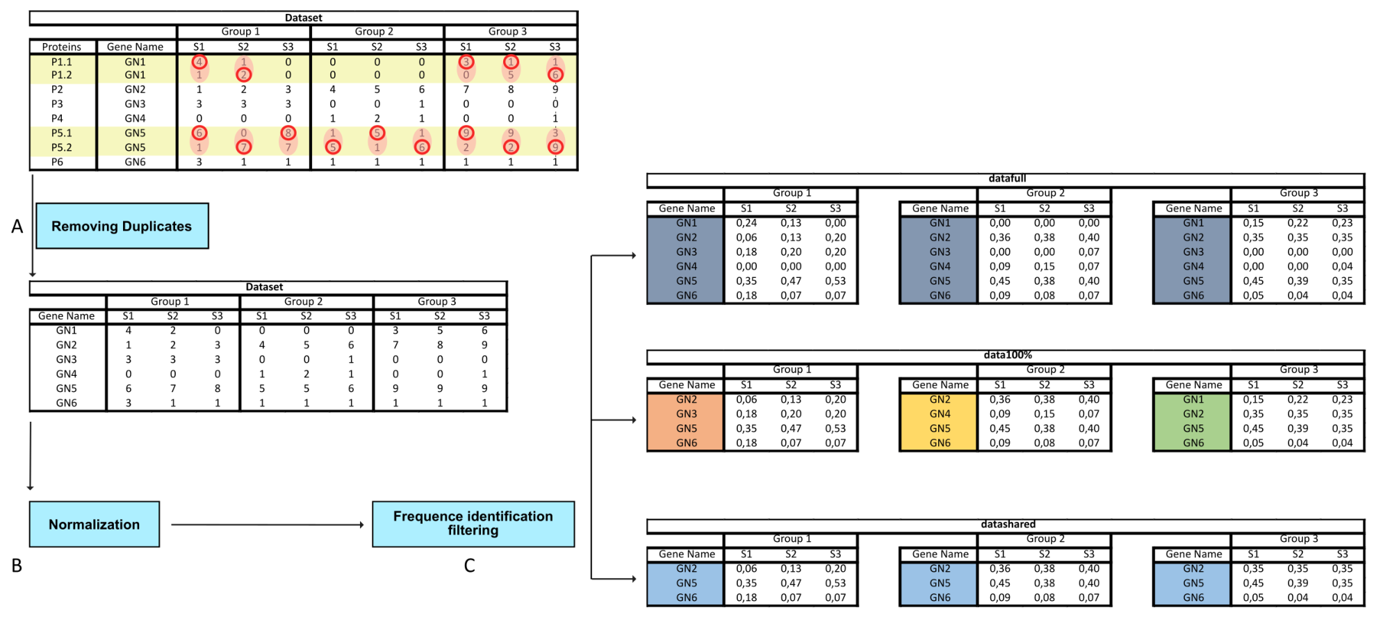
Figure 4.
Multidimensional scaling (MDS) plot. Using the results of the MANOVA analysis, PiProteline generates an MDS plot to rapidly assess how well the characterized profiles, as well as the differentially expressed proteins, discriminate between the groups/conditions under study (C, PD, PG). Each point represents an individual sample, and distances between points reflect their pairwise dissimilarities. The first two dimensions (MDS1 and MDS2) account for the major variance, clearly highlighting the separation between the experimental groups/conditions.
Figure 4.
Multidimensional scaling (MDS) plot. Using the results of the MANOVA analysis, PiProteline generates an MDS plot to rapidly assess how well the characterized profiles, as well as the differentially expressed proteins, discriminate between the groups/conditions under study (C, PD, PG). Each point represents an individual sample, and distances between points reflect their pairwise dissimilarities. The first two dimensions (MDS1 and MDS2) account for the major variance, clearly highlighting the separation between the experimental groups/conditions.
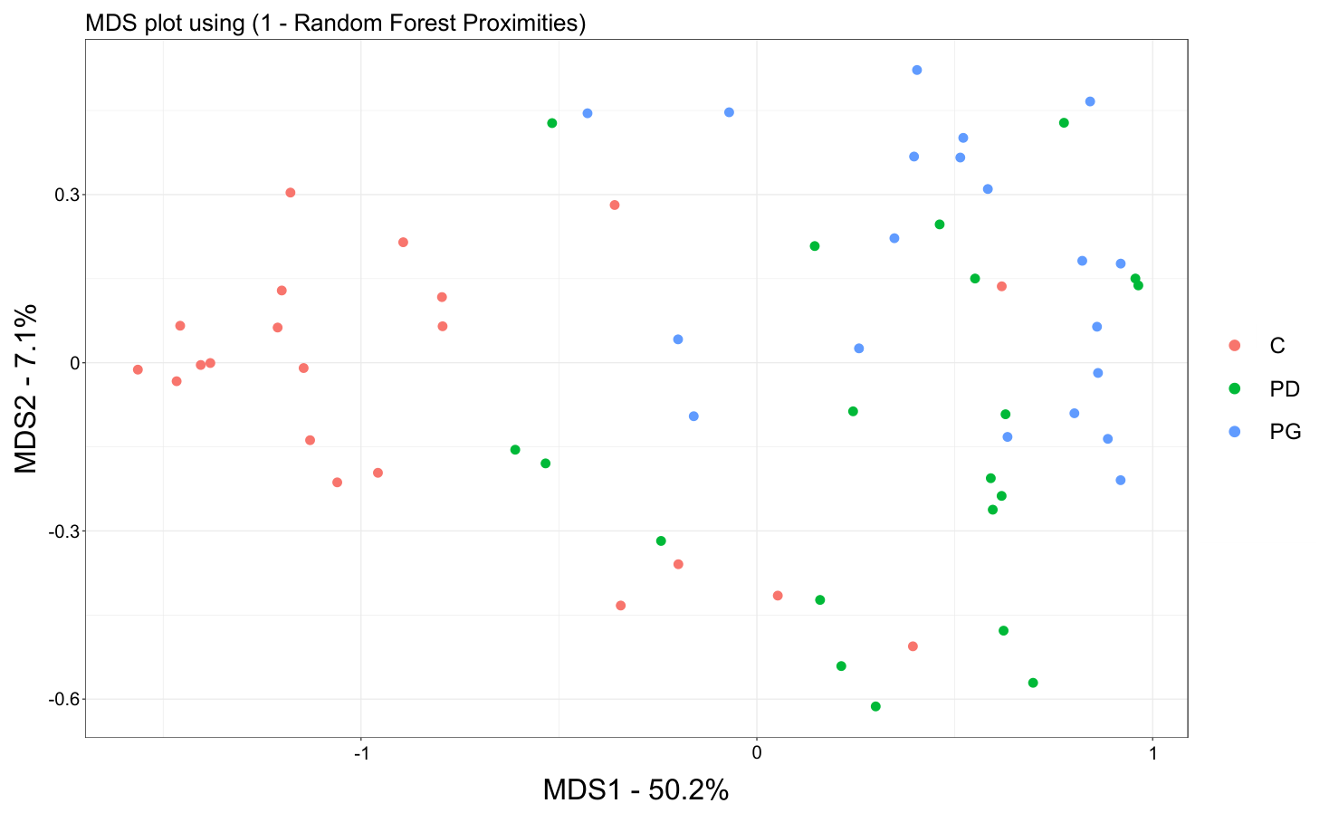
Figure 5.
Volcano Plot. Representative volcano plot from the comparison between control (C) and Parkinson’s disease (PD) groups. The x-axis represents the fold change (FC), while the y-axis displays the . Proteins that pass the significance thresholds (|FC| and adj.p-value) are highlighted in red (up-regulated in C) or blue (down-regulated in C), respectively.
Figure 5.
Volcano Plot. Representative volcano plot from the comparison between control (C) and Parkinson’s disease (PD) groups. The x-axis represents the fold change (FC), while the y-axis displays the . Proteins that pass the significance thresholds (|FC| and adj.p-value) are highlighted in red (up-regulated in C) or blue (down-regulated in C), respectively.
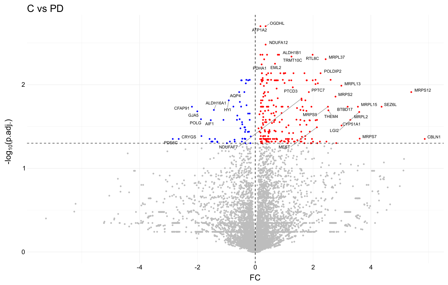
Figure 6.
Functional enrichment analysis. A) Example of biological processes (BP) enriched using the single-profile enrichment strategy. BP terms are arranged in a tree structure according to the number of shared proteins, while the corresponding bars are proportional to the number of proteins (normalized 0–100) identified for a given BP in each color-coded group/condition. B) Example of a bar plot showing the most enriched BPs (exclusive) in pairwise comparisons (using DEPs or hubs and bottlenecks). The x-axis reports the ratio of proteins within the set, and bar color indicates the false discovery rate (FDR), where darker blue shades correspond to more significant terms.
Figure 6.
Functional enrichment analysis. A) Example of biological processes (BP) enriched using the single-profile enrichment strategy. BP terms are arranged in a tree structure according to the number of shared proteins, while the corresponding bars are proportional to the number of proteins (normalized 0–100) identified for a given BP in each color-coded group/condition. B) Example of a bar plot showing the most enriched BPs (exclusive) in pairwise comparisons (using DEPs or hubs and bottlenecks). The x-axis reports the ratio of proteins within the set, and bar color indicates the false discovery rate (FDR), where darker blue shades correspond to more significant terms.
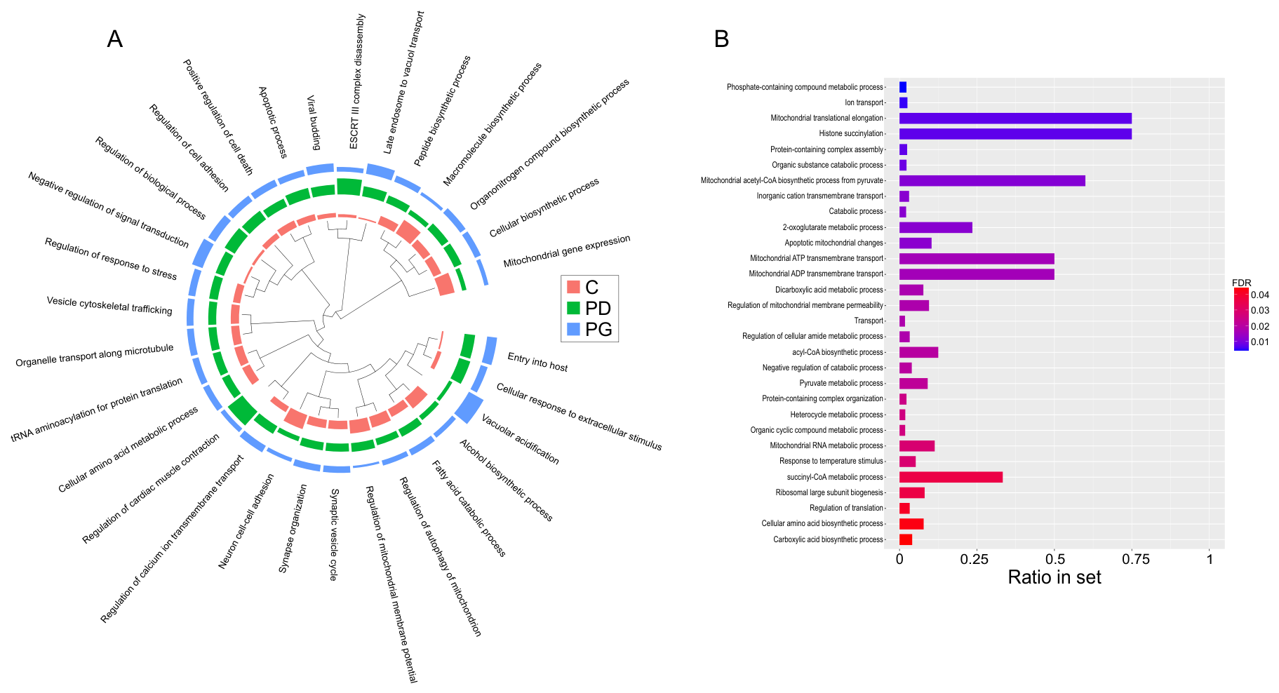

Table 1.
Classification of hub proteins based on network centrality measures. The table reports whether each protein exceeds the 75th percentile threshold for Betweenness and Centroid centrality in groups G1 and G2. Based on these metrics, proteins are classified as non-specific hubs, specific hubs, centrality specific hubs, or not hubs. The same classification applies to bottlenecks when considering betweenness and bridging centralities.
Table 1.
Classification of hub proteins based on network centrality measures. The table reports whether each protein exceeds the 75th percentile threshold for Betweenness and Centroid centrality in groups G1 and G2. Based on these metrics, proteins are classified as non-specific hubs, specific hubs, centrality specific hubs, or not hubs. The same classification applies to bottlenecks when considering betweenness and bridging centralities.
| Proteins | Betweenness over 75th percentile in G1 |
Centroid over 75th percentile in G1 |
Betweenness over 75th percentile in G2 |
Centroid over 75th percentile in G2 |
G1 Hub type |
|---|---|---|---|---|---|
| P1 | yes | yes | yes | yes | non-specific hub |
| P2 | yes | yes | yes | no | specific hub |
| P3 | yes | yes | no | no | centrality specific hub |
| P4 | yes | no | no | no | not hub |
Disclaimer/Publisher’s Note: The statements, opinions and data contained in all publications are solely those of the individual author(s) and contributor(s) and not of MDPI and/or the editor(s). MDPI and/or the editor(s) disclaim responsibility for any injury to people or property resulting from any ideas, methods, instructions or products referred to in the content. |
© 2026 by the authors. Licensee MDPI, Basel, Switzerland. This article is an open access article distributed under the terms and conditions of the Creative Commons Attribution (CC BY) license (http://creativecommons.org/licenses/by/4.0/).
Copyright: This open access article is published under a Creative Commons CC BY 4.0 license, which permit the free download, distribution, and reuse, provided that the author and preprint are cited in any reuse.


