
Submitted:
21 July 2026
Posted:
22 July 2026
You are already at the latest version
Abstract
Corn serves as one of China’s core staple crops which guarantees national grain security, yet frequent pest infestation severely cuts crop yields. Conventional crop protection measures suffer from low operating efficiency and inevitable environmental contamination, meanwhile existing mainstream detection algorithms are restricted by insufficient identification precision and high computational overhead. Targeting the above drawbacks, this research develops an improved RMS-YOLOv11 detection framework to achieve high-precision identification of corn pest individuals. The RFB component is embedded into the backbone’s feature extraction terminal of native YOLOv11 to strengthen feature extraction capacity for tiny pest targets; MobileNetV2 lightweight architecture is introduced to reduce model computational overhead; the original standard Conv layer is replaced with self-designed Conv-SWS module to balance multi-scale feature enhancement for targets with different sizes. Quantitative experimental outcomes reveal that the proposed RMS-YOLOv11 achieves 90% detection precision, 83% recall, 89.1% mAP@50, 65.5% mAP@75 and 59.3% mAP@50-95. These five indicators are separately raised by 3.1%, 4%, 4.5%, 2.4% and 3.6% compared with vanilla YOLOv11, and the proposed framework achieves better overall detection metrics against Faster-RCNN, SSD and other mainstream YOLO variants. Grad-CAM thermal visualization results verify that the optimized network can precisely lock the actual pest area and remedy the original network’s deficiency of inadequate feature attention toward small-size targets. The presented detection scheme supplies reliable technical support for field corn pest prevention and control and bears practical significance to safeguard domestic corn production safety.
Keywords:
YOLOv11
; corn pests
; object detection
; detection accuracy
1. Introduction
As a critical staple food resource in China, corn had a planting area hitting 671 million mu alongside an annual output of 589.83 billion jin by 2024. Apart from human daily consumption, corn also acts as fundamental raw material for livestock feed and deep industrial processing, occupying an irreplaceable position in domestic food security guarantee system. Pests such as corn borer and cotton borer larva would bring drastic yield decline to corn planting [1], while timely pest inspection can grasp disaster development trend to arrange targeted prevention and lower economic losses. Traditional pest management mainly depends on artificial field inspection and chemical pesticide spraying, which comes with low working efficiency and severe ecological pollution problems, creating urgent demand for eco-friendly and high-efficiency automated pest detection technologies.
With the continuous progress of sensing and wireless communication techniques, field pest monitoring gradually evolves toward automatic and remote management modes. Installing pheromone-based intelligent trapping devices in farmland can finish automatic image acquisition and transmit picture data to remote monitoring terminals via wireless signal; certain wireless sensor equipment can reach 93% detection accuracy to realize unattended field monitoring and cut manual cost [2]. Nevertheless, acquired pest images still rely heavily on manual classification and statistics, limiting overall inspection efficiency. Advancements in computer science push classic machine learning algorithms including SVM and random forest into pest identification domains. Relevant scholars adopted machine learning frameworks to complete farmland pest monitoring tasks [3], and another research obtained 89.1% identification accuracy for olive fruit fly with random forest algorithm [4]. Still, such traditional learning methods require manually customized feature engineering, resulting in weaker robustness and generalization performance under complex field surroundings compared with deep learning-based solutions.
Deep learning technology gradually dominates current pest detection research, getting rid of manual feature design constraints and enabling autonomous extraction of high-level semantic information from pest images. Existing deep-learning-based pest detectors fall into two mainstream categories: two-stage detection algorithms represented by Faster-RCNN and Mask-RCNN, and single-stage frameworks centered on YOLO and SSD families.
Multiple previous studies optimized two-stage detection architectures for agricultural pest scenarios: Chen et al. put forward an anchor-free rotating two-stage detection network AF-R2PN, lifting AP value by 2.3% against horizontal detection benchmarks [5]; Wang et al. combined improved lightweight UNet with Mask-RCNN core ideas to implement pest semantic segmentation and boost detailed feature processing performance [6]; Mu et al. constructed edge-computing oriented two-stage detector for micro pest identification with outstanding F1 metric [7]. Other researchers also applied improved RCNN and SVM hybrid structures to improve pest classification precision [8,9,10,11]. Even though these two-stage models acquire decent detection precision, redundant network structure leads to slow inference speed and limits field deployment potential. In contrast, single-stage detectors skip region proposal generation steps to cut computational overhead and show potential for deployment on field hardware.
YOLO series algorithms stand out among single-stage detection networks with balanced precision and inference efficiency, and their lightweight variants can be deployed directly on embedded hardware and mobile terminals. A large number of existing literatures continuously optimize different YOLO versions toward agricultural pest identification: Liu refined YOLOv3 via image pyramid to raise tomato pest detection precision and speed [12]; Pang substituted conventional NMS with Diou-NMS to upgrade YOLOv4 and reached 92.86% mAP with 12.22 ms single-image detection latency [13]; Li added attention block and optimized loss function on YOLOv5 to get 96.51% average precision [14]; successive improvements on YOLOv7/YOLOv8/YOLOv10/YOLO11 also achieved prominent promotion on pest detection indicators [15,16,17,18,19,20]. The verified superiority of YOLO algorithms greatly facilitates the development of intelligent agricultural pest detection.
Against the above research background, this paper designs a lightweight high-precision detection network oriented to complex field corn pest scenarios, with four core research objectives: first, construct a standardized multi-category corn pest dataset with sufficient sample volume; second, improve original YOLOv11 via RFB, MobileNetV2 and Conv-SWS three modules to strengthen small-target detection and realize network lightweight; third, validate model effectiveness and generalization through comprehensive contrast and ablation experiments; fourth, supply feasible intelligent detection solutions for smart agricultural corn pest monitoring scenarios.
2. Materials and Methods
2.1. Dataset
All 4,547 field images of corn pests used in this study were collected from 2023 to 2024, and all model training, comparison and generalization verification experiments were conducted from 2025 to 2026.The corn pest dataset adopted in this study contains 4,547 field-shot images covering nine typical corn pest species. All raw images were captured under complex natural field environments with variable illumination, leaf occlusion, dense tiny pest clusters and mixed pest coexistence scenarios. All samples were randomly split into training, validation and test subsets following a fixed 7:2:1 ratio. This article supplements Table 1, quantifying the names of each type of pest and the exact total number of labelled boxes for that category. Significant unbalanced distribution of annotated objects across classes exists, which is naturally caused by inconsistent pest population density in actual corn fields. During the training phase, online data augmentation strategies including random scaling and rotation are applied to alleviate the negative impact of class imbalance on model training.Figure 1a displays category name and sample graph of nine pests while Figure 1b describes sample quantity distribution for each pest type.
Most images in the dataset contain multi-target scenes: a single image may simultaneously contain multiple individuals of the same pest species or mixed individuals of different pest taxa. No multi-target samples are discarded during dataset construction, so the dataset can fully restore the complex overlapping and occlusion conditions of real farmland, which helps improve the multi-target detection robustness of the model.
Complete Dataset Annotation Workflow:
(1)Image pre-filtering: Excessively blurred, overexposed and distorted images were manually eliminated, retaining 4,547 valid field images for subsequent annotation. All reserved images were unified to a consistent resolution standard, and invalid low-quality samples were excluded.
(2)Initial manual labeling: The whole labeling work was undertaken by three postgraduate students with basic digital image processing capabilities. All annotators received systematic pre-training on morphological discrimination of nine corn pests, mastering the differentiation standards between target pests and background interference such as crop leaves, soil and weeds. The LabelImg annotation tool was used to draw bounding boxes for all visible pest individuals and export YOLO-format TXT label files.
(3)Inter-annotator cross verification: To evaluate labeling consistency, 20% of all images were randomly selected as a verification subset, and re-labeled independently by all three annotators. Two core consistency metrics were calculated: average bounding box IoU between different annotators reached 0.92, and the category label agreement rate was 96.4%. All samples with large box position deviation or conflicting category judgments were marked for subsequent expert review to eliminate subjective labeling bias.
(4)Full expert secondary validation: Two professional plant protection experts from the College of Agriculture conducted full-image inspection on all annotated samples. With reference to standard pest specimen atlases, the experts corrected misclassified pest labels, missing pest bounding boxes and false annotations on background impurities. Confusing juvenile larvae and morphologically similar pest individuals were uniformly re-calibrated to guarantee taxonomic accuracy of all labels.
(5)Final format quality inspection: The authors conducted a full check of matching relations between images and annotation files. Empty label files without any targets were deleted, and formatting errors including out-of-bounds coordinate values and duplicate overlapping bounding boxes were fixed, generating the final standardized dataset for model training and testing.
2.2. RMS-YOLO
YOLO algorithm is recognized as classic single-stage detection architecture for real-time target identification, and updated YOLOv11 further optimizes network structure with better lightweight property and multi-scene adaptability, hence this paper selects YOLOv11 as baseline network. The original YOLOv11 has obvious defects in practical application: insufficient feature extraction capacity for small-size pest targets, excessive computational complexity, bulky model volume and unsatisfactory detection accuracy. Aiming at these drawbacks, this research completes targeted network optimization to build RMS-YOLOv11, and Figure 2 and Figure 3 separately present structural layout of primitive YOLOv11 and improved RMS-YOLOv11:
(1) Embed RFB module into the tail of YOLOv11 backbone feature extraction branch. Multi-branch convolution plus dilated convolution inside RFB expands network receptive field under the premise of controlling parameter quantity and enhances feature extraction ability for tiny pest objects;
(2) Introduce MobileNetV2 containing inverted residual and linear bottleneck structure alongside global average pooling design. Such lightweight design cuts total parameters and calculation cost effectively, and helps reduce computational burden for edge terminal deployment;
(3) Replace native standard Conv layer with self-developed Conv-SWS module. Featured slicing and adaptive enhancement operations help the network capture feature information of both large and small targets to realize balanced multi-scale identification performance.
2.2.1. RFB
Even though YOLO series gains wide usage in object detection tasks, its native feature extraction structure still needs further optimization for practical application. Plenty of existing researches proposed various feature enhancement modules to fix such defects: Liu teams built joint feature extraction unit for infrared ship inspection [21], another research introduced global feature fusion block to lift overall feature extraction performance [22], Mamba-based dual-branch structure and dense connection plus attention hybrid modules are also verified effective for feature optimization [23,24]. This work embeds RFB component at backbone output end to boost small-target feature learning capacity, and Figure 4 displays internal construction of RFB module.
RFB is composed of multi-branch ordinary convolution and dilated convolution two parts. For multi-branch part, 1 × 1 convolution firstly compresses channel dimension and aggregates shallow-layer feature information, followed by multi-size convolution to collect local detail features; another round of 1 × 1 convolution without activation unifies output channel dimension of each branch. Dilated convolution expands receptive field range without increasing parameter number and retains high-resolution feature data. The subsequent feature fusion operation combines two-branch output to acquire final RFB feature mAP.
Given an input feature tensor
where C denotes the number of channels, and represent the height and width of the feature mAP, respectively. First, 1 × 1 convolution is used for channel compression and feature integration:
where and are the weight and bias of the 1 × 1 convolution kernel, σ is the activation function, and ∗ denotes the standard convolution operation. Multi-branch multi-scale convolution is then performed to capture local details at different scales:
The multi-branch features are concatenated and dimensionally aligned using 1 × 1 convolution without activation:
where denotes channel-wise concatenation.Dilated convolution with dilation rate r is defined as:
which expands the receptive field to k + (k − 1) (r − 1) for kernel size k without increasing parameters. Finally, the multi-branch features and dilated convolution features are fused to obtain the RFB output:
The model proposed in this paper significantly enhances the network’s feature extraction and perception capabilities for small targets by integrating the multi-branch structure and dilated convolution characteristics of RFB.
2.2.2. MobileNetV2
Classical convolution networks like ResNet and VGG own excellent identification capability but suffer from parameter redundancy and huge computational overhead, limiting their deployment on resource-limited mobile embedded devices. MobileNet family is proposed to construct low-latency lightweight network, MobileNetV1 relies on depthwise separable convolution to shrink model size yet brings partial precision loss after lightweight processing [25]; MobileNetV3 upgrades feature dimension transformation mode and introduces SE attention to improve detection performance [26]. Different from above variants, this paper chooses MobileNetV2 as lightweight backbone, which adopts depth separable convolution, inverse residual unit and linear bottleneck design: it expands feature channel to obtain abundant high-dimensional semantic information first and reduces dimension with linear activation to avoid low-dimensional feature loss, finally outputs results after global average pooling. Such design drastically cuts calculation load and realizes lightweight deployment without severe precision drop, and Figure 5 shows MobileNetV2 internal structure.
2.2.3. Conv-SWS
Convolution unit is the core feature extraction component of YOLO network, but built-in standard Conv exists fixed receptive field and uniform feature weight distribution defects, making it hard to adapt multi-scale pest detection under complex farmland background and causing low feature utilization efficiency. Many scholars optimized convolution structure for detection promotion: SPDConv, SD-Conv and improved Swin-based convolution all prove effective for feature loss reduction [27,28,29]. Combined with SimAM attention mechanism, this research constructs Conv-SWS convolution module via feature slicing optimization.
The original global SimAM calculates pixel difference relying on full feature mAP statistics, leading small targets with similar feature value to global average to be ignored as background information. The slicing operation in Conv-SWS divides feature mAP into multiple local blocks and calculates attention weight based on block-level pixel statistics: small pest targets own larger difference against block mean value to obtain higher enhancement weight, while large-size targets keep stable feature response after feature fusion. The specific segmentation process is shown in Figure 6.
Given an input feature mAP
the feature mAP is uniformly sliced into N × N local blocks:
where each block is
For each block , the energy function of each pixel (x,y) is calculated as:
where and are the channel-wise mean and standard deviation of the block (i,j), and λ is a small constant to avoid division by zero.
The attention weight is obtained by:
Small targets have larger energy values and obtain higher weights, while large targets maintain stable recognition.
First, standard convolution extracts basic features:
Then, element-wise weighting is performed with sliced attention:
where denotes element-wise multiplication.
Finally, batch normalization is applied to obtain the output of Conv-SWS:
This mechanism balances the feature enhancement of large and small targets and improves multi-scale detection performance.
3. Results
3.1. Experimental Environment and Training Configuration
The experimental environment and training configuration parameters used in this paper are shown in Table 2 and Table 3, respectively.
All experimental training and testing tasks are finished on Ubuntu22.04 operating system with Intel Xeon Platinum 8358P CPU and RTX3090 GPU, CUDA12.1 is equipped for hardware acceleration while Pytorch2.1.0 and Python3.10 form experimental software framework. Model training selects SGD optimizer, setting weight decay as 0.0005, momentum coefficient 0.937, initial learning rate 0.001 and batch size 32 with total 220 training epochs; dataset partitioning follows fixed 7:2:1 train-val-test split rule, precision, recall, mAP@50, mAP@75 and mAP@50-95 serve as unified evaluation metrics for all comparison experiments.
All experiments adopt a fixed input image size of 640 × 640 pixels, and low-quality images with resolution lower than 320 × 320 are eliminated during preprocessing. Online data augmentation is applied during training with fixed probabilities: horizontal flip p=0.5, ±15° random rotation p=0.4, random center crop p=0.3, and 0.7–1.3× random scaling p=0.4; vertical flip, random brightness and noise augmentation are not used in this study.
For model inference and evaluation, a unified confidence threshold of 0.25 is adopted to filter low-confidence predictions, and the NMS IoU threshold is set to 0.65. Consistent with COCO evaluation standards, mAP@50 uses an IoU threshold of 0.5, mAP@75 uses 0.75, and mAP@50-95 averages results over IoU thresholds ranging from 0.50 to 0.95 with a step of 0.05. The anchor boxes are generated via k-means clustering (k=9) on the training set, matched with positive samples when IoU ≥ 0.5. An early stopping strategy with a patience of 30 epochs is activated; training terminates early if the validation mAP@50 shows no improvement for 30 consecutive epochs, and the checkpoint with the highest validation mAP@50 is retained.
All comparative, ablation and cross-model experiments were repeated three times independently with identical hyperparameters. We adopted paired t-test to conduct statistical significance analysis on Precision, Recall and mAP@0.50-0.95 between the baseline YOLOv11 and the proposed RMS-YOLOv11. The 95% confidence interval (CI) of each metric was calculated to quantify the fluctuation range of experimental results, which provides statistical evidence for the performance gaps observed between models.
3.2. Measurement Indicators
Five quantitative indicators including Precision, Recall, mAP@50, mAP@75 and mAP@50-95 are selected to measure network detection performance. The methods for calculating these metrics are detailed in formulas (1)–(4).Precision and Recall reflect single-category target identification correctness via TP/FP/FN statistical calculation; AP equals integral of PR curve for single pest class, and mAP means average AP value across all categories. mAP@50 and mAP@75 adopt IoU threshold 0.5 and 0.75 separately while mAP@50-95 averages results under multi-IoU thresholds to evaluate model comprehensive generalization capacity. All computational formulas of indicators keep consistent with original definition, nine pest categories correspond to n = 9 in mAP calculation.
3.3. Ablation Experiment
This study first established the baseline model of YOLOv11, and then quantitatively analyzed its impact on various model indicators by introducing the three innovation points proposed in this paper (denoted as B for RFB, M for MobileNetV2, and S for Conv_SWS) to measure its significance. Table 4 presents the experimental data of the ablation experiment, and Figure 7 shows the P-R curve of the ablation experiment.
Ablation test takes vanilla YOLOv11 as baseline, separately adding RFB (R), MobileNetV2 (M), Conv-SWS (S) single module, dual-module combination and three-module integration to explore each component’s independent and synergistic optimization effect, concrete experimental data are listed in Table 4 and P-R curve is displayed in Figure 7. Experimental statistics indicate single module can bring limited performance gain, dual-module combination achieves obvious indicator improvement and three components used simultaneously yields the most balanced overall detection performance: final precision reaches 90%, recall 83%, mAP@50 89.1%, mAP@75 65.5%, mAP@50-95 59.3%, verifying three modules own complementary optimization characteristic.
Paired t-test results show that all performance indicators of RMS-YOLOv11 are significantly higher than the vanilla YOLOv11 at the 95% confidence level (p < 0.05), which statistically verifies the effectiveness of the three proposed modules.
3.4. Comparison of Similar Improvements
3.4.1. Comparative Experiment with RFB
In this subsection, the impact of similar improvements to RFB on the model will be explored, including EMCA_attention [30], BSAM [31], MSAM, EMA_attention [32], and SimAM. The results are shown in Table 5.
As can be seen from the experimental data of each group in Table 5, the overall performance of the baseline M+S model is moderate. After introducing improvements such as EMCA, BSAM, MSAM, EMA, and SimAM, the performance of the models has its own advantages and disadvantages: EMA_attention and SimAM have increased the accuracy rate to 88.4%, which is superior to other attention modules; BSAM has slightly improved in some indicators, but the overall improvement is limited. The remaining improvement plans only saw a slight increase in a few indicators, and some even declined. The proposed method achieves competitive results across all evaluation metrics, with a precision of 90%, and the remaining metrics being 83%, 89.1%, 65.5%, and 59.3%, surpassing the baselines and various attention-enhanced models. The results indicate that the method proposed in this paper achieves good outcomes across multiple dimensions, has clear advantages, and maintains more stable overall performance. Paired t-test analysis at the 95% confidence level (p < 0.05) shows that our integrated module achieves moderately improved overall detection metrics compared with other similar attention modules tested, and random training fluctuations have limited impact on the comparative results.
3.4.2. Comparative Experiment of MobileNetV2
In this subsection, the influence of different network structures will be explored. The comparison structures are MobileNetV3 [33], MobileNetV4, and StarNet [34]. The experimental results are shown in Table 6.
From the data comparison in Table 6, it can be seen that the accuracy rate of R + S as the baseline model reaches 89.4%, and its overall performance is superior to its improved versions combined with networks such as MobileNetV3, MobileNetV4, and StarNet. All the indicators of the latter have declined to varying degrees, among which the StarNet-related combination has the most significant decline. The accuracy rate is as low as 82.3%. The method proposed in this paper performs well, with an accuracy rate of 90%, an improvement of 0.6% compared to the baseline R + S, and achieves 83%, 89.1%, 65.5%, and 59.3% respectively in the other four indicators, outperforms most comparative lightweight backbones on comprehensive indicators. This indicates that the method proposed in this paper has achieved a comprehensive improvement in all dimensional indicators while maintaining high core accuracy, verifying its effectiveness. Statistical results of paired t-test (95% CI, p < 0.05) illustrate that the MobileNetV2 backbone adopted in this work yields mild performance advantages over MobileNetV3, MobileNetV4 and StarNet under the same experimental setup.
3.4.3. Comparative Experiments of Conv_SWS
In this subsection, the impact of different improvements to Conv on the model will be explored, including AKConv, DSConv [35], DynamicConv [36], DynamicBnAct and LDConv [37]. The results are shown in Table 7.
As can be seen from the comparison of various indicators in Table 7, after introducing different convolution and modules respectively on the basis of R + M, the overall performance has been improved to varying degrees. Among them, R + M + DynamicConv and R + M + DynamicBnAct performed outstandingly, with an accuracy rate reaching 89.7%, outperforming improved methods such as AKConv, DSConv, and LDConv. The method proposed in this paper demonstrates overall better performance, achieving an accuracy of 90%, while matching or surpassing other improved schemes on other reference metrics; compared with other improvement modules, Ours maintains high values while ensuring stability, without noticeable performance fluctuations, achieves balanced and stable performance compared with other convolution improvement modules, which to some extent validates the effectiveness and superiority of the proposed method. The paired t-test at 95% confidence interval (p < 0.05) suggests that the proposed Conv-SWS module brings modest balanced performance gains relative to other optimized convolution units.
3.5. Error Analysis
The comparison of the two normalized confusion matrices shows that the overall performance of the second model is better. Only Spodoptera frugiperda remains unchanged, but the precision rates of most pest categories have significantly improved. The misjudgment distribution of background categories is more reasonable, and the overall classification accuracy and consistency are significantly better than the first one. Among them, Figure 8 refers to the confusion matrix of YOLOv11, and Figure 9 refers to the confusion matrix of RMS-YOLOv11.
3.6. Comparison with Other Models
To evaluate the performance of the YOLO model in the task of corn pest detection, this study benchmarked it against nine mainstream object detection networks. The constructed control system covers representative works of both two-stage and single-stage detectors, including Faster-RCNN, SSD, RT-DETR, and the v5, v6, v8, v9m, v10m and v11 of the YOLO series. The detailed quantitative comparison results are presented in Table 8.
It can be seen from the comparison of various indicators in Table 8 that Faster-RCNN performs outstandingly in recall rate, but its precision rate and mAP are relatively low. The indicators of SSD and RT-DETR are relatively balanced and are generally at a medium level. The YOLO series has a significant overall accuracy advantage. Among them, YOLOv8 and YOLOv13 have relatively high precision rates, while YOLOv9m and YOLOv11 perform better in detection at high IoU thresholds. However, there is still room for improvement in terms of comprehensive indicators. The method proposed in this paper (Ours) shows the best performance in terms of precision, mAP@50, mAP@75 and mAP@50-95, which are 90%, 89.1%, 65.5% and 59.3% respectively. Only the recall rate is slightly lower than that of faster-rCNN. Overall, this method gains favorable comprehensive detection accuracy and multi-scale robustness compared with mainstream detectors and presents competitive detection capacity. Paired t-test statistics with a 95% confidence threshold (p < 0.05) demonstrate that our model obtains mild performance advantages over most compared two-stage and single-stage detectors on core evaluation metrics.
3.7. Model Feasibility Analysis
Heat mAPs serve as essential tools for the visual analysis of deep learning models, exemplified by Grad-CAM type heat mAPs. These visualizations enable the verification of whether a model has effectively learned relevant target features, rather than being influenced by extraneous factors such as background and texture. They facilitate the rapid identification of model deficiencies, particularly in instances of misjudgments or missed detections, by revealing whether the model is focusing on inappropriate areas. Additionally, heat mAPs contribute to the optimization of network architecture, refinement of dataset annotations, and removal of noisy samples, thereby enhancing the model’s interpretability. This approach addresses the black box problem inherent in deep learning and provides an intuitive foundation for model tuning and experimental analysis.
In this paper, the Grad-CAM method is adopted to compare YOLOv11 with RMS-YOLOv11. The specific test results are shown in Figure 10.
Figure 10 presents a comparison of the heat mAP visualizations for the original corn pest samples, YOLOv11, and RMS-YOLOv11. The heat mAP generated by YOLOv11 exhibits scattered areas of concern, indicating inadequate feature capture for small targets and weakly characteristic pests. In contrast, the thermal mAP produced by RMS-YOLOv11 demonstrates significant improvements, allowing for a more precise and comprehensive focus on the target pest areas. The feature response is more concentrated, and the positioning accuracy is enhanced. This advancement moderately enhances the model’s ability to detect and locate corn pests in complex environments, thereby validating the feasibility and effectiveness of the proposed improved strategy.
3.8. Model Generalization Capability Verification Experiment
The generalization ability of a model determines whether it can work stably and reliably on new data that has never been seen before, and it is the core indicator for measuring the practicality of a model. Strong generalization ability means that the model will not overfit the training data, and can effectively deal with noise, distribution differences and complex changes in real scenarios, avoiding failure in practical applications. Conversely, models with poor generalization only perform well in the training set, but their accuracy drops sharply after implementation, lacking practical value. Good generalization ability is directly related to the robustness, deployment effect and long-term availability of the model, and it is the key for algorithms to move from the laboratory to engineering applications. In this experiment, a rice pest dataset and a tomato disease dataset were selected to verify the generalisation ability of RMS-YOLOv11.
Two training strategies are adopted for rice pest and tomato disease datasets: training from scratch and transfer learning initialized with weights pre-trained on the maize pest dataset. For transfer learning, the backbone layers are frozen for the first 50 epochs, followed by full-network fine-tuning with a reduced initial learning rate of 0.0005, while all other hyperparameters remain consistent with the maize pest experiment.
3.8.1. Rice Pests
The dataset utilized in this section of the experiment comprises 4573 samples, encompassing 11 common types of rice pests. These samples are partitioned into a training set, a validation set, and a test set in a ratio of 7:2:1. The parameters of the experimental environment and training configuration are consistent with those established in the previous experiment. The results of the experiment are presented in Table 9 and Table 10.
Experiments validate the cross-task adaptability of RMS-YOLOv11 for rice pest detection. As shown in Table 9 and Table 10, RMS-YOLOv11 achieves competitive detection results on the rice pest dataset, with overall P, R, mAP@50, mAP@75 and mAP@50-95 of 86.6%, 85.1%, 90.8%, 83.3% and 76.5%, respectively. The proposed method yields consistent metric improvements over the original YOLOv11, showing favorable adaptability to diverse pest detection tasks under different agricultural scenarios.
3.8.2. Tomato Disease
The dataset used in this experiment consists of 3046 images, including five common types of tomato diseases, and is divided into training, validation, and test sets in a 7:2:1 ratio. The experimental environment and training configuration parameters are the same as in previous experiments. The experimental results are shown in Table 11 and Table 12.
Further experiments verify the cross-task applicability of RMS-YOLOv11 for tomato disease identification. As summarized in Table 11 and Table 12, the proposed model obtains P, R, mAP@50, mAP@75 and mAP@50-95 values of 80.7%, 74.8%, 84.0%, 76.2% and 70.9%, respectively. Compared with vanilla YOLOv11, RMS-YOLOv11 achieves steady performance gains in tomato disease recognition, demonstrating reliable detection capacity and practical application potential for agricultural disease identification tasks.
Obvious domain gaps exist across the three agricultural datasets, including differences in target morphology, background texture, lighting conditions and target scale distribution. Although RMS-YOLOv11 achieves steady performance gains across the three datasets, such results merely demonstrate limited cross-task adaptability, and the model still lacks robust cross-domain generalization for completely different agricultural scenes.
3.9. Missed Detection Inspection
Missed detection refers to the phenomenon where the YOLO model does not output a detection box for the actual existing target in the image during reasoning, resulting in the target not being recognized. It is one of the core errors in object detection. The causes include the target being too small, severe occlusion, blurred features, and an excessively high confidence threshold, etc. Missed detections directly reflect the model’s ability to recall the target. The higher the missed detection rate, the worse the model’s practicality. By analyzing the characteristics of the missed detection targets, the data set can be optimized, the anchor frames adjusted, the network structure and loss function improved, the model’s detection ability for difficult samples enhanced, and the integrity and reliability of the detection system ensured. In this experiment, RMS-YOLOV11 was applied to the task of corn pest detection to verify and analyze the missed detection situation of the model. The test results are shown in Figure 11.
Figure 11 illustrates that YOLOv11 exhibits notable missed detections, particularly for small targets such as peach aphids and grubs, as well as for densely clustered targets that are not fully identified. Additionally, the confidence levels for some detected targets are relatively low. In contrast, RMS-YOLOv11 significantly reduces missed detections, more completely frames targets, has higher confidence, and has improved detection capability for dense and small pests, demonstrating its superiority in agricultural pest identification scenarios.
3.10. Deploy
We developed a complete master-slave embedded intelligent pest monitoring terminal and carried out systematic field machine tests. The hardware platform takes Raspberry Pi 4B as the main controller and GD32F103 as slave chips, equipped with a 12 MP CSI camera, multi-environment sensors, 4G communication module and touch human-machine interaction screen (Figure 12: Internal assembly structure of the integrated monitoring equipment; Figure 13: Overall exterior of the pest monitoring station). Multi-thread software scheduling based on LVGL separates sensor sampling, local display, model inference and cloud transmission tasks, supporting automatic, manual and rain-induced sleep working modes. Figure 14 shows the main touchscreen homepage with functional entries for equipment status, captured images and system information, while Figure 15 presents the touch interface under manual operation mode, where users can manually activate insect trapping, photographing and all execution components via on-screen virtual buttons. The lightweight RMS-YOLOv11 model can run real-time inference locally on Raspberry Pi without cloud GPU support. Sensor data and pest recognition results are uploaded to the cloud via MQTT and HTTP protocols, realizing remote equipment control and long-term pest trend analysis. The complete set of hardware and field test data constitutes experimental evidence, which to a certain extent verifies the real-time inference capability and field practical value of the proposed model.
4. Conclusions
To enable timely and accurate corn pest detection, this paper proposes RMS-YOLOv11 integrated with RFB, MobileNetV2 and Conv-SWS modules. RFB expands receptive fields to improve small-target detection. MobileNetV2 reduces model parameters and computation for efficient inference. Conv-SWS strengthens multi-scale pest feature representation.
On our self-built dataset, the model achieves 90% precision, 83% recall, 89.1% mAP@50, 65.5% mAP@75 and 59.3% mAP@50-95. Statistical analysis with paired t-test (p < 0.05, 95% CI) confirms that RMS-YOLOv11 obtains statistically significant performance gains over vanilla YOLOv11, Faster-RCNN, SSD and other mainstream YOLO variants on all core evaluation metrics. Compared with these models, RMS-YOLOv11 gains higher precision and mAP values and shows evident improvements for tiny and multi-scale pest targets in complex field scenes.
The proposed RMS-YOLOv11 achieves accurate corn pest detection suitable for field application scenarios. It reduces reliance on manual inspection and excessive pesticide use, effectively cutting labor and chemical control costs. This technology helps timely pest control and minimizes yield losses, bringing considerable economic benefits to corn cultivation. Meanwhile, it supports the development of eco-friendly and intelligent plant protection in modern agriculture.
Corn pest species are diverse and full data collection remains challenging. In future research, we will focus on major harmful pests, expand dataset categories and further optimize the model to adapt to field pest control demands.
Author Contributions
Conceptualization, methodology design, software development and original draft preparation, M.D.; investigation and quantitative analysis, Y.W.; validation and data curation, J.L.; visualization and project administration, Y.N.; writing—review and editing, supervision and funding acquisition, Y.L. All authors have read and agreed to the published version of the manuscript.
Funding
This research was supported by the following projects: (1) Natural Science Foundation of Heilongjiang Province: Research on Smart Irrigation System (No. JJ2025XQ0050); (2) “Double First-Class” Discipline Collaborative Innovation Achievement Project of Heilongjiang Province: R&D of Intelligent Integrated Irrigation Head (No. LJGXCG2024-F06); (3) “Double First-Class” Discipline Collaborative Innovation Achievement Project of Heilongjiang Province: Research and Development of Intelligent Irrigation Controller (No. LJGXCG2023-063).
Data Availability Statement
The data presented in this study are available on request from the corresponding author due to the confidentiality of the field monitoring equipment prototype developed in this research.
Conflicts of Interest
Author Yong Liu was employed by Heilongjiang East Water Saving Equipment Company. The remaining authors declare that the research was conducted in the absence of any commercial or financial relationships that could be construed as a potential conflict of interest.
References
- Li, X.; Liu, Y.; Pei, Z.; Tong, G.; Yue, J.; Li, J.; Dai, W.; Xu, H.; Shang, D.; Ban, L. The Efficiency of Pest Control Options against Two Major Sweet Corn Ear Pests in China. Insects 2023, 14(12), 929. [Google Scholar] [CrossRef] [PubMed]
- Rustia, D.J.A.; Lin, C.E.; Chung, J.Y.; Zhuang, Y.J.; Hsu, J.C.; Lin, T.T. Application of an image and environmental sensor network for automated greenhouse insect pest monitoring. J. Asia-Pac. Entomol. 2020, 23(1), 17–28. [Google Scholar] [CrossRef]
- Chithambarathanu, M.; Jeyakumar, M.K. Survey on crop pest detection using deep learning and machine learning approaches. Multimed. Tools Appl. 2023, 82(27), 42277–42310. [Google Scholar] [CrossRef] [PubMed]
- Molina-Rotger, M.; Morán, A.; Miranda, M.A.; Alorda-Ladaria, B. Remote fruit fly detection using computer vision and machine learning-based electronic trap. Front. Plant Sci. 2023, 14. [Google Scholar] [CrossRef] [PubMed]
- Chen, T.J.; Chen, H.B.; Du, J.M.; Wang, R.J.; Zhang, M.; Zhang, W. TSAF-Net: a rotated two-stage Cnaphalocrocis medinalis damage detection method based on anchor-free arbitrary-oriented proposal network. Pest Manag. Sci. 2024, 80(9), 4604–4616. [Google Scholar] [CrossRef] [PubMed]
- Wang, F.K.; Huang, Y.Q.; Huang, Z.C.; Shen, H.; Huang, C.; Qiao, X.; Qian, W.Q. MRUNet: A two-stage segmentation model for small insect targets in complex environments. J. Integr. Agric. 2023, 22(4), 1117–1130. [Google Scholar] [CrossRef]
- Mu, J.L.; Sun, L.L.; Ma, B.; Liu, R.F.; Liu, S.X.; Hu, X.L.; Zhang, H.J.; Wang, J.X. TFEMRNet: A Two-Stage Multi-Feature Fusion Model for Efficient Small Pest Detection on Edge Platforms. Agriengineering 2024, 6(4), 4688–4703. [Google Scholar] [CrossRef]
- Huang, H.S.; Deng, J.Z.; Lan, Y.B.; Yang, A.; Deng, X.L.; Zhang, L.; Wen, S.; Jiang, Y.; Suo, G.Y.; Chen, P.C. A two-stage classification approach for the detection of spider mite- infested cotton using UAV multispectral imagery. Remote Sens. Lett. 2018, 9(10), 933–941. [Google Scholar] [CrossRef]
- Wu, X.C.; Liu, Y.L.; Xing, M.J.; Yang, C.; Hong, S.Y. Image segmentation for pest detection of crop leaves by improvement of regional convolutional neural network. Sci. Rep. 2024, 14(1). [Google Scholar] [CrossRef] [PubMed]
- Deng, F.M.; Mao, W.; Zeng, Z.Q.; Zeng, H.; Wei, B.Q. Multiple Diseases and Pests Detection Based on Federated Learning and Improved Faster R-CNN. IEEE Trans. Instrum. Meas. 2022, 17. [Google Scholar] [CrossRef]
- Li, K.R.; Duan, L.J.; Deng, Y.J.; Liu, J.L.; Long, C.F.; Zhu, X.H. Pest Detection Based on Lightweight Locality-Aware Faster R-CNN. Agronomy-Basel 2024, 14(10). [Google Scholar] [CrossRef]
- Liu, J.; Wang, X.W. Tomato Diseases and Pests Detection Based on Improved Yolo V3 Convolutional Neural Network. Front. Plant Sci. 2020, 11. [Google Scholar] [CrossRef] [PubMed]
- Pang, H.T.; Zhang, Y.T.; Cai, W.M.; Li, B.; Song, R.Y. A real-time object detection model for orchard pests based on improved YOLOv4 algorithm. Sci. Rep. 2022, 12(1). [Google Scholar] [CrossRef] [PubMed]
- Li, K.S.; Wang, J.C.; Jalil, H.; Wang, H. A fast and lightweight detection algorithm for passion fruit pests based on improved YOLOv5. Comput. Electron. Agric. 2023, 204. [Google Scholar] [CrossRef]
- Yang, Z.J.; Feng, H.L.; Ruan, Y.P.; Weng, X. Tea Tree Pest Detection Algorithm Based on Improved Yolov7-Tiny. Agriculture-Basel 2023, 13(5). [Google Scholar] [CrossRef]
- Gan, X.; Cao, S.K.; Wang, J.; Wang, Y.; Hou, X. YOLOv8-DBW: An Improved YOLOv8-Based Algorithm for Maize Leaf Diseases and Pests Detection. Sensors 2025, 25(15). [Google Scholar] [CrossRef] [PubMed]
- Zhang, L.J.; Ding, G.C.; Li, C.R.; Li, D.M. DCF-Yolov8: An Improved Algorithm for Aggregating Low-Level Features to Detect Agricultural Pests and Diseases. Agronomy-Basel 2023, 13(8). [Google Scholar] [CrossRef]
- Yuan, W.X.; Lan, L.F.; Xu, J.Y.; Sun, T.T.; Wang, X.H.; Wang, Q.M.; Hu, J.N.; Wang, B.J. Smart Agricultural Pest Detection Using I-YOLOv10-SC: An Improved Object Detection Framework. Agronomy-Basel 2025, 15(1). [Google Scholar] [CrossRef]
- Tian, Y.N.; Wang, S.H.; Li, E.; Yang, G.D.; Liang, Z.Z.; Tan, M. MD-YOLO: Multi-scale Dense YOLO for small target pest detection. Comput. Electron. Agric. 2023, 213. [Google Scholar] [CrossRef]
- Qiang, J.; Zhao, L.; Wang, H.M.; Xu, T.Q.; Jia, Q.H.; Sun, L.X. YOLO-PEST: a novel rice pest detection approach based on YOLOv5s. Plant Methods 2025, 21(1). [Google Scholar] [CrossRef] [PubMed]
- Liu, Y.J.; Li, C.F.; Fu, G.H. PJ-YOLO: Prior-Knowledge and Joint-Feature-Extraction Based YOLO for Infrared Ship Detection. J. Mar. Sci. Eng. 2025, 13(2). [Google Scholar] [CrossRef]
- Liu, Y.B.; Cheng, X.; Xu, N.; Wang, L.Y.; Wang, X.; Zhong, X. MFAE-YOLO: Multifeature Attention-Enhanced Network for Remote Sensing Images Object Detection. Ieee Trans. Geosci. Remote Sens. 2025, 63. [Google Scholar] [CrossRef]
- Feng, J.J.; Yan, S.L.; Sang, H.R.; Chen, H.; Xu, S.Q.; Cai, N.; Zhou, Y.H. SSOD-YOLO: Mamba-Driven Feature Extraction With Adaptive Feature Enhancement for Small-Object Detection in Space. Ieee Aerosp. Electron. Syst. Mag. 2026, 41(3), 46–64. [Google Scholar] [CrossRef]
- Tian, Y.N.; Wang, S.H.; Li, E.; Yang, G.D.; Liang, Z.Z.; Tan, M. MD-YOLO: Multi-scale Dense YOLO for small target pest detection. Comput. Electron. Agric. 2023, 213. [Google Scholar] [CrossRef]
- Zhang, C.; Yang, T.; Yang, J. Image Recognition of Wind Turbine Blade Defects Using Attention-Based MobileNetv1-YOLOv4 and Transfer Learning. Sensors 2022, 22(16). [Google Scholar] [CrossRef] [PubMed]
- Duan, Z.L.; Liu, H.Y. Improving Network Structure for Efficient Classification Network Based on MobileNetV3. Ieee Access 2025, 13, 191296–191308. [Google Scholar] [CrossRef]
- Gu, Z.C.; Zhu, K.; You, S.T. YOLO-SSFS: A Method Combining SPD-Conv/STDL/IM-FPN/SIoU for Outdoor Small Target Vehicle Detection. Electronics 2023, 12(18). [Google Scholar] [CrossRef]
- Zhu, J.X.; Qin, C.; Choi, D. YOLO-SDLUWD: YOLOv7-based small target detection network for infrared images in complex backgrounds. Digit. Commun. Netw. 2025, 11(2), 269–279. [Google Scholar] [CrossRef]
- Chen, X.; Liu, T.; Han, K.; Jin, X.J.; Wang, J.X.; Kong, X.T.; Yu, J.L. TSP-yolo-based deep learning method for monitoring cabbage seedling emergence. Eur. J. Agron. 2024, 157. [Google Scholar] [CrossRef]
- Wang, Q.; Wu, B.; Zhu, P.; Li, P.; Zuo, W.; Hu, Q. ECA-Net: Efficient Channel Attention for Deep Convolutional Neural Networks. 2020 IEEE/CVF Conference on Computer Vision and Pattern Recognition (CVPR), Seattle, WA, USA, 2020; pp. 11531–11539. [Google Scholar] [CrossRef]
- Zhu, L.; Wang, X.; Ke, Z.; Zhang, W.; Lau, R. BiFormer: Vision Transformer with Bi-Level Routing Attention. 2023 IEEE/CVF Conference on Computer Vision and Pattern Recognition (CVPR), Vancouver, BC, Canada, 2023; pp. 10323–10333. [Google Scholar] [CrossRef]
- Ouyang, D.; et al. Efficient Multi-Scale Attention Module with Cross-Spatial Learning. ICASSP 2023—2023 IEEE International Conference on Acoustics, Speech and Signal Processing (ICASSP), Rhodes Island, Greece, 2023; pp. 1–5. [Google Scholar] [CrossRef]
- Howard, A.; et al. Searching for MobileNetV3. 2019 IEEE/CVF International Conference on Computer Vision (ICCV), Seoul, Korea (South), 2019; pp. 1314–1324. [Google Scholar] [CrossRef]
- Ma, X.; Dai, X.; Bai, Y.; Wang, Y.; Fu, Y. Rewrite the Stars. 2024 IEEE/CVF Conference on Computer Vision and Pattern Recognition (CVPR), Seattle, WA, USA, 2024; pp. 5694–5703. [Google Scholar] [CrossRef]
- Nascimento, M. G. D.; Prisacariu, V.; Fawcett, R. DSConv: Efficient Convolution Operator. 2019 IEEE/CVF International Conference on Computer Vision (ICCV), Seoul, Korea (South), 2019; pp. 5147–5156. [Google Scholar] [CrossRef]
- Han, K.; Wang, Y.; Guo, J.; Wu, E. ParameterNet: Parameters are All You Need for Large-Scale Visual Pretraining of Mobile Networks. 2024 IEEE/CVF Conference on Computer Vision and Pattern Recognition (CVPR), Seattle, WA, USA, 2024; pp. 15751–15761. [Google Scholar] [CrossRef]
- Zhang, X.; Song, Y.Z.; Song, T.T.; Yang, D.G.; Ye, Y.C.; Zhou, J.; Zhang, L.M. LDConv: Linear deformable convolution for improving convolutional neural networks. Image Vis. Comput. 2024, 149. [Google Scholar] [CrossRef]
- Wang, L.H.; Shi, W.P.; Tang, Y.H.; Liu, Z.Z.; He, X.K.; Xiao, H.Y.; Yang, Y. Transfer Learning-Based Lightweight SSD Model for Detection of Pests in Citrus. Agronomy-Basel 2023, 13(7). [Google Scholar] [CrossRef]
Figure 1.
(a) shows the images and names of all pest categories, while (b) presents the corresponding sample distribution.
Figure 1.
(a) shows the images and names of all pest categories, while (b) presents the corresponding sample distribution.
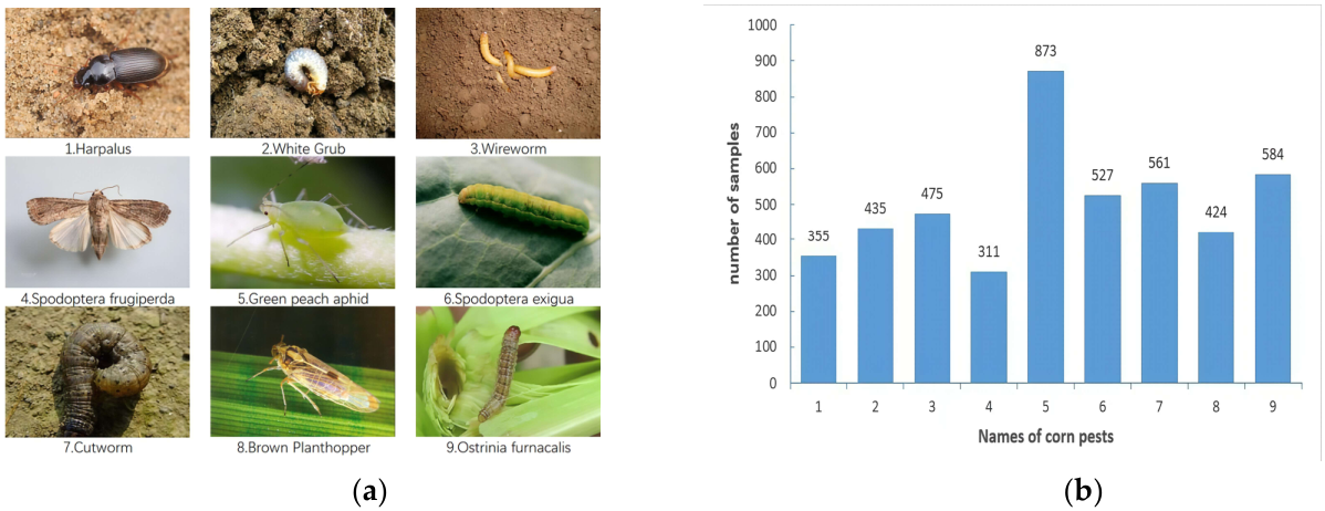
Figure 2.
YOLOv11 model architecture.
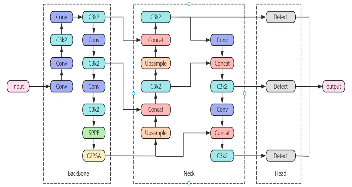
Figure 3.
RMC-YOLOv11 model architecture.
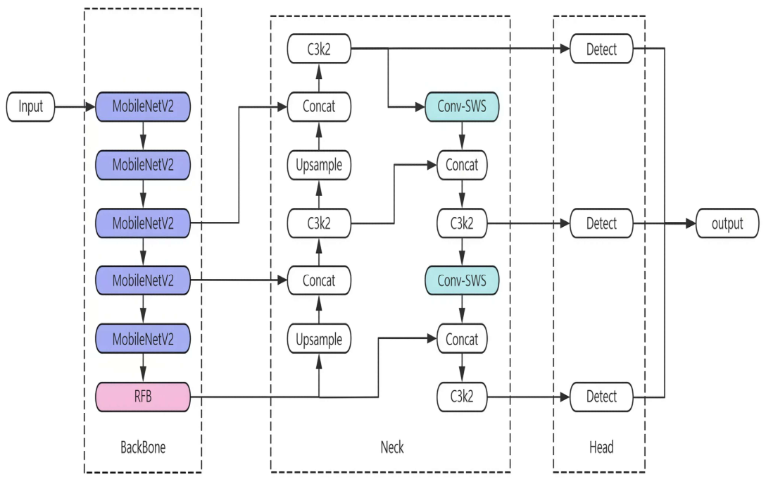
Figure 4.
RFB structure.
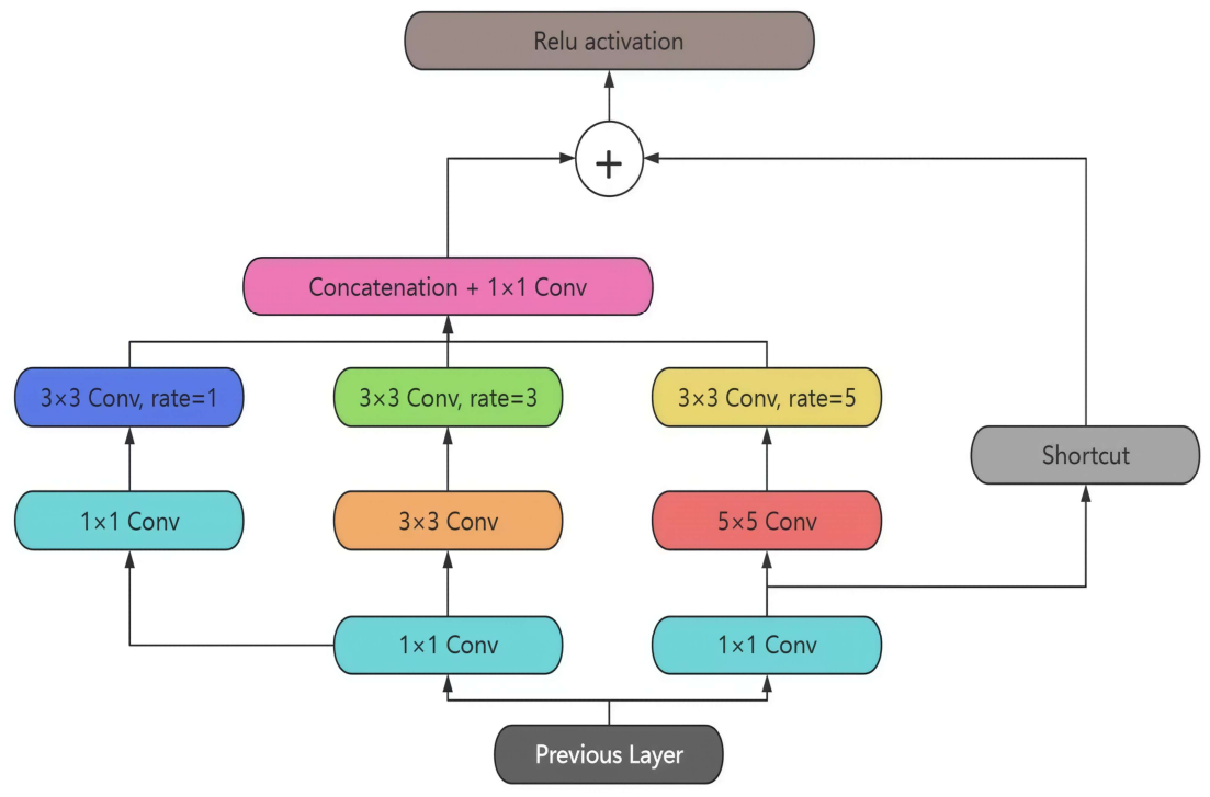
Figure 5.
Structure diagram of MobileNetV2.
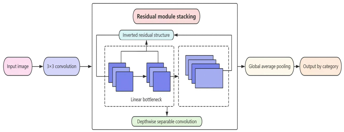
Figure 6.
shows the slicing process diagram.
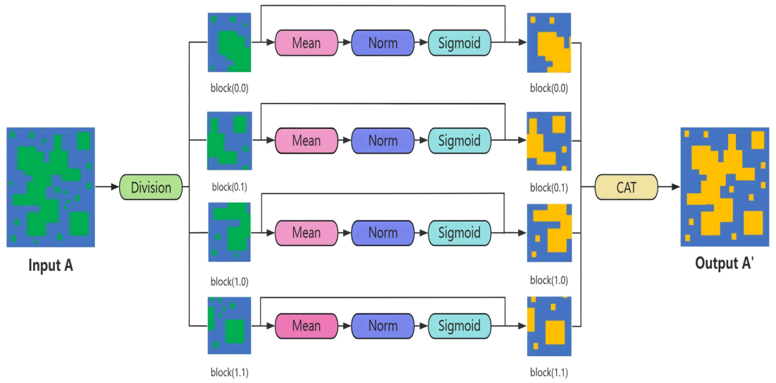
Figure 7.
The P-R curve graph of the ablation experiment.
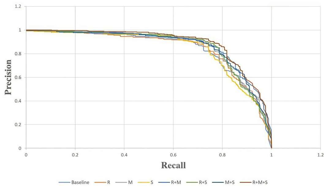
Figure 8.
The confusion matrix of YOLOv11.
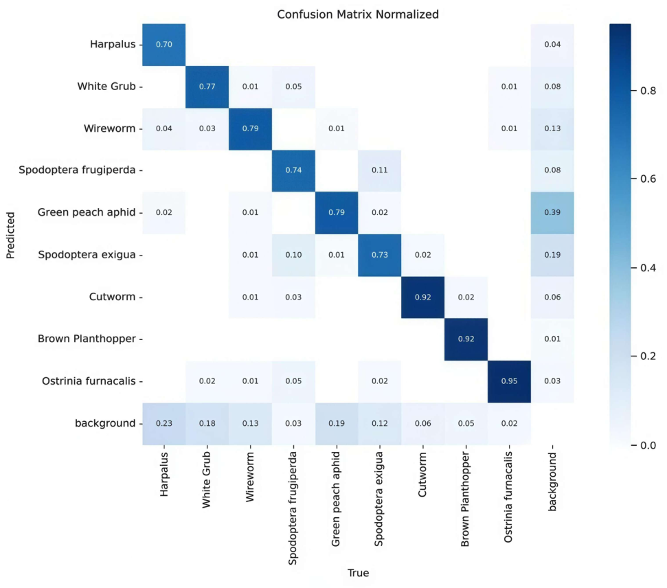
Figure 9.
The confusion matrix of RMS-YOLOv11.
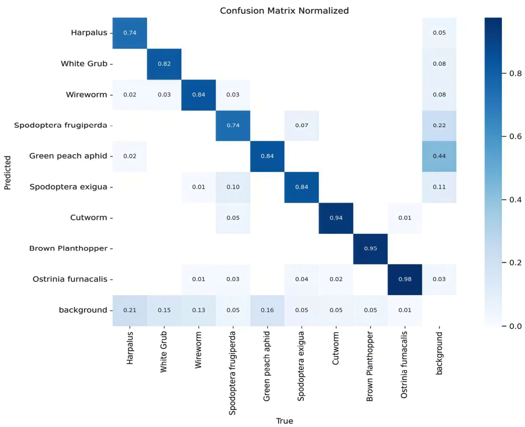
Figure 10.
Heat mAP of the model.
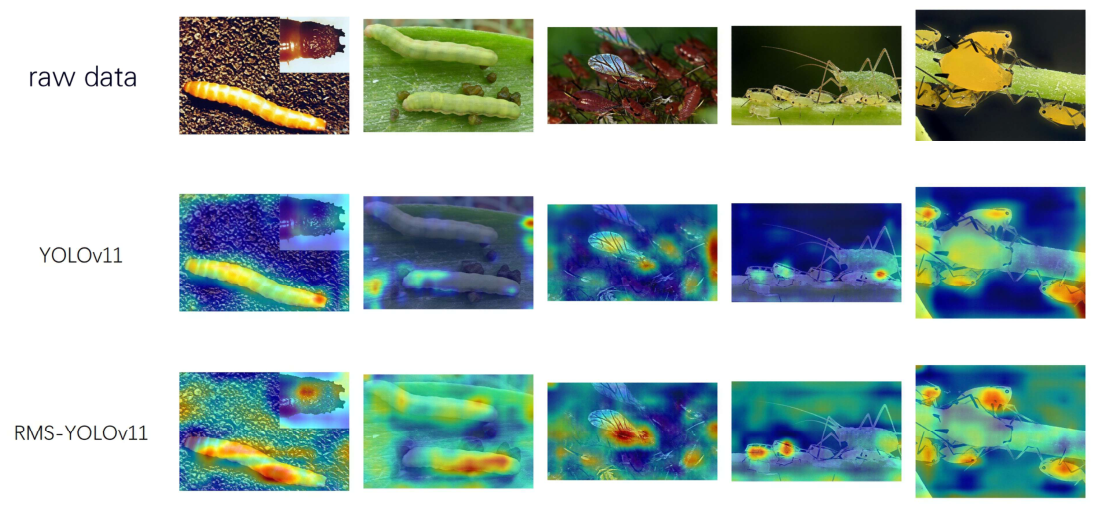
Figure 11.
Results of missed detections.
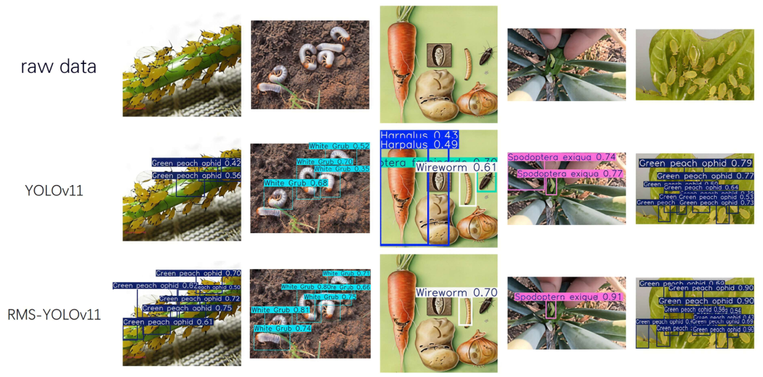
Figure 12.
Internal assembly structure of intelligent pest monitoring station.
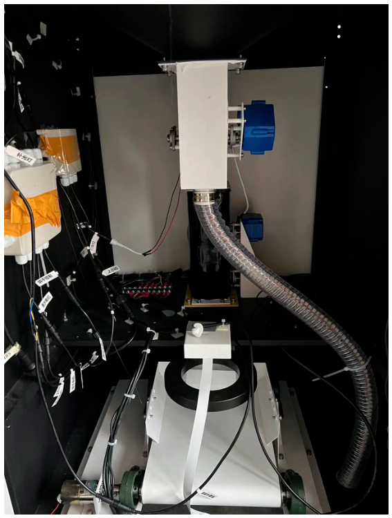
Figure 13.
Overall physical appearance of the monitoring terminal.
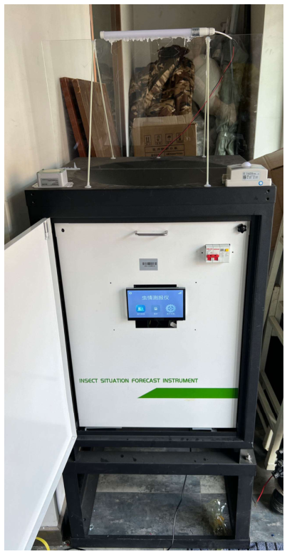
Figure 14.
Main touch screen home interface of the device.
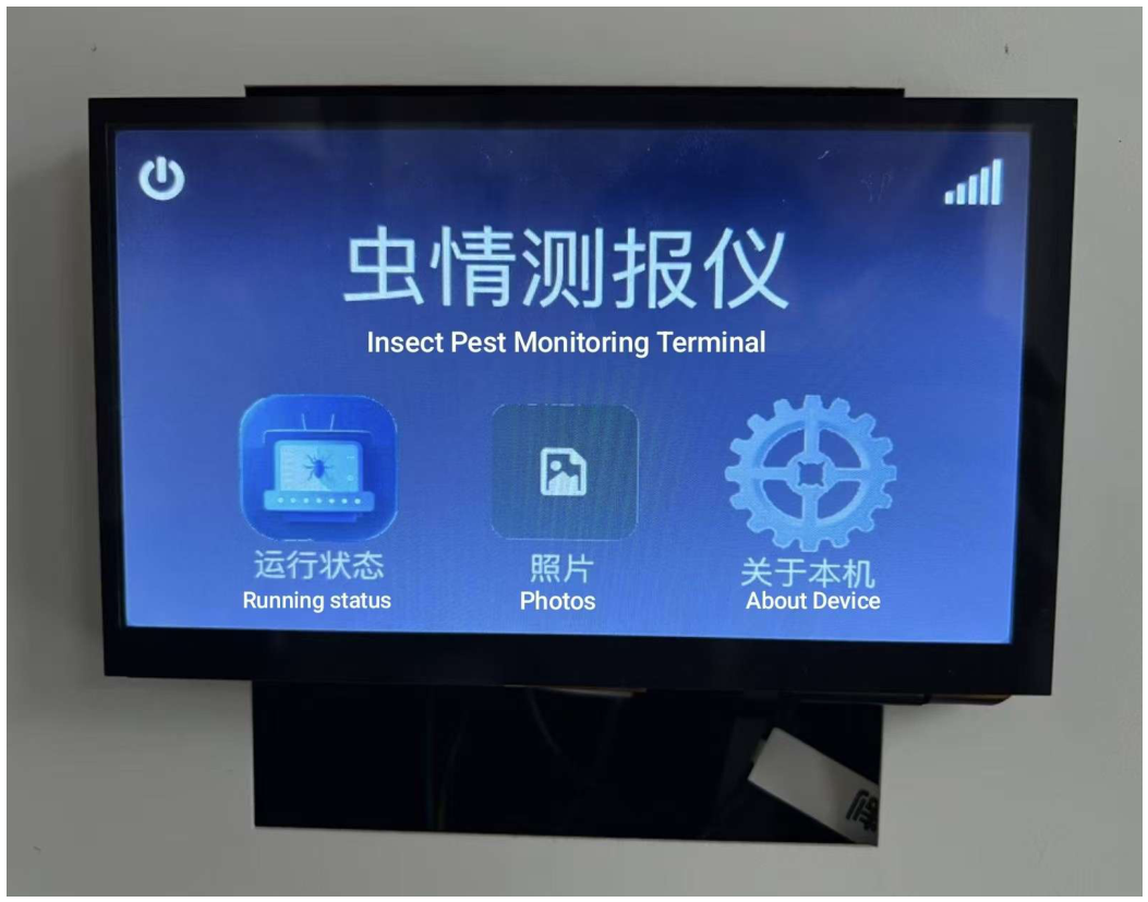
Figure 15.
Touchscreen interface under manual working mode.
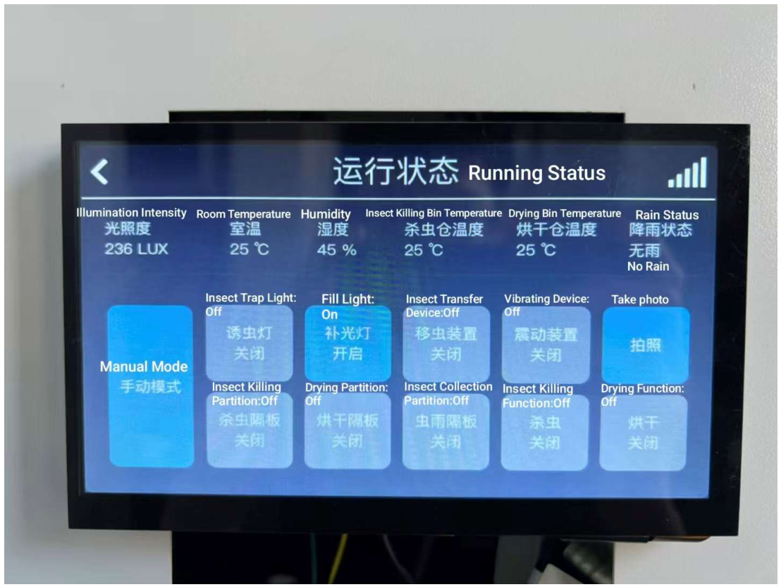

Table 1.
The exact number of annotations for each type of target.
| Names of corn pests | Number of annotation boxes |
| 1 | 402 |
| 2 | 676 |
| 3 | 661 |
| 4 | 358 |
| 5 | 1400 |
| 6 | 566 |
| 7 | 600 |
| 8 | 507 |
| 9 | 596 |
Table 2.
Experimental Environment.
| Item | Setup |
|---|---|
| OS | Ubuntu22.04 |
| CPU | Intel(R) Xeon(R) Platinum 8358P |
| GPU | NVIDIA GeForce RTX3090 |
| GPU acclerator | CUDA12.1 |
| Deep learning frame | Pytorch 2.1.0 |
| Scipting language | Python 3.10 |
Table 3.
Training Configuration.
| Setting | Value |
|---|---|
| Weight decay | 0.0005 |
| Momentum factor | 0.937 |
| learning rate | 0.001 |
| Batch | 32 |
| epochs | 220 |
| Optimizer | SGD |
Table 4.
Ablation experiment data.
| R | M | S | P | R | mAP@50 | mAP@75 | mAP@50-95 |
|---|---|---|---|---|---|---|---|
| 0.869 | 0.79 | 0.846 | 0.631 | 0.557 | |||
| √ | 0.857 | 0.803 | 0.846 | 0.609 | 0.551 | ||
| √ | 0.882 | 0.819 | 0.862 | 0.632 | 0.566 | ||
| √ | 0.881 | 0.793 | 0.845 | 0.603 | 0.552 | ||
| √ | √ | 0.868 | 0.832 | 0.878 | 0.658 | 0.587 | |
| √ | √ | 0.894 | 0.781 | 0.865 | 0.644 | 0.576 | |
| √ | √ | 0.867 | 0.822 | 0.866 | 0.64 | 0.573 | |
| √ | √ | √ | 0.9 | 0.83 | 0.891 | 0.655 | 0.593 |
Table 5.
Experimental results on similar improvements of RFB.
| Name | P | R | mAP@50 | mAP@75 | mAP@50-95 |
|---|---|---|---|---|---|
| M + S | 0.867 | 0.822 | 0.866 | 0.64 | 0.573 |
| M + S + EMCA_attention | 0.867 | 0.826 | 0.874 | 0.623 | 0.563 |
| M + S + BSAM | 0.851 | 0.845 | 0.866 | 0.665 | 0.582 |
| M + S + MSAM | 0.874 | 0.81 | 0.856 | 0.643 | 0.576 |
| M + S + EMA_attention | 0.884 | 0.812 | 0.872 | 0.642 | 0.573 |
| M + S + SimAM | 0.884 | 0.795 | 0.859 | 0.632 | 0.567 |
| Ours | 0.9 | 0.83 | 0.891 | 0.655 | 0.593 |
Table 6.
Experimental Results of Different Structures.
| Name | P | R | mAP@50 | mAP@75 | mAP@50-95 |
|---|---|---|---|---|---|
| R + S | 0.894 | 0.781 | 0.865 | 0.644 | 0.576 |
| R + S + MobileNetV3 | 0.861 | 0.795 | 0.845 | 0.621 | 0.558 |
| R + S + MobileNetV4 | 0.865 | 0.771 | 0.839 | 0.6 | 0.551 |
| R + S + StarNet | 0.858 | 0.746 | 0.811 | 0.571 | 0.519 |
| Ours | 0.9 | 0.83 | 0.891 | 0.655 | 0.593 |
Table 7.
Experimental Results on different improvements of Conv.
| Name | P | R | mAP@50 | mAP@75 | mAP@50-95 |
|---|---|---|---|---|---|
| R + M | 0.868 | 0.832 | 0.878 | 0.658 | 0.587 |
| R + M + AKConv | 0.88 | 0.83 | 0.88 | 0.652 | 0.593 |
| R + M + DSConv | 0.892 | 0.807 | 0.879 | 0.655 | 0.581 |
| R + M + DynamicConv | 0.897 | 0.814 | 0.875 | 0.631 | 0.588 |
| R + M + DynamicBnAct | 0.897 | 0.812 | 0.873 | 0.642 | 0.576 |
| R + M + LDConv | 0.88 | 0.83 | 0.88 | 0.652 | 0.593 |
| Ours | 0.9 | 0.83 | 0.891 | 0.655 | 0.593 |
Table 8.
Experimental Data of Different Networks.
| Name | P | R | mAP@50 | mAP@75 | mAP@50-95 |
|---|---|---|---|---|---|
| Faster-RCNN | 0.621 | 0.891 | 0.878 | 0.472 | 0.489 |
| SSD | 0.808 | 0.809 | 0.858 | 0.544 | 0.515 |
| RT-DETR | 0.87 | 0.768 | 0.793 | 0.554 | 0.517 |
| YOLOv5 | 0.853 | 0.797 | 0.844 | 0.584 | 0.538 |
| YOLOv6 | 0.824 | 0.758 | 0.812 | 0.544 | 0.509 |
| YOLOv8 | 0.874 | 0.801 | 0.863 | 0.608 | 0.552 |
| YOLOv9m | 0.853 | 0.797 | 0.85 | 0.617 | 0.571 |
| YOLOv10m | 0.868 | 0.785 | 0.847 | 0.593 | 0.557 |
| YOLOv11 | 0.869 | 0.79 | 0.846 | 0.631 | 0.557 |
| Ours | 0.9 | 0.83 | 0.891 | 0.655 | 0.593 |
Table 9.
Results of YOLOv11 on the rice pest dataset.
| Class | P | R | mAP@50 | mAP@75 | mAP@50-95 |
|---|---|---|---|---|---|
| all | 0.84 | 0.784 | 0.846 | 0.774 | 0.704 |
| Curculionidae | 0.899 | 0.709 | 0.786 | 0.7 | 0.664 |
| Delphacidae | 0.811 | 0.822 | 0.862 | 0.766 | 0.73 |
| Cicadellidae | 0.829 | 0.546 | 0.703 | 0.569 | 0.503 |
| Phlaeothripidae | 0.88 | 0.513 | 0.701 | 0.446 | 0.455 |
| Cecidomyiidae | 0.915 | 0.955 | 0.968 | 0.941 | 0.837 |
| Hesperiidae | 0.964 | 0.974 | 0.993 | 0.972 | 0.855 |
| Crambidae | 0.9 | 0.982 | 0.949 | 0.918 | 0.817 |
| Chloropidae | 0.772 | 0.706 | 0.789 | 0.77 | 0.707 |
| Ephydridae | 0.838 | 0.857 | 0.89 | 0.84 | 0.743 |
| Noctuidae | 0.834 | 0.619 | 0.778 | 0.712 | 0.669 |
| Thripidae | 0.599 | 0.938 | 0.891 | 0.878 | 0.76 |
Table 10.
Results of RMS-YOLOv11 on the rice pest dataset.
| Class | P | R | mAP@50 | mAP@75 | mAP@50-95 |
|---|---|---|---|---|---|
| all | 0.866 | 0.851 | 0.908 | 0.833 | 0.765 |
| Curculionidae | 0.911 | 0.762 | 0.848 | 0.772 | 0.715 |
| Delphacidae | 0.835 | 0.87 | 0.89 | 0.839 | 0.79 |
| Cicadellidae | 0.845 | 0.624 | 0.789 | 0.634 | 0.579 |
| Phlaeothripidae | 0.788 | 0.592 | 0.747 | 0.534 | 0.501 |
| Cecidomyiidae | 0.951 | 1 | 0.995 | 0.952 | 0.853 |
| Hesperiidae | 0.95 | 1 | 0.989 | 0.972 | 0.857 |
| Crambidae | 0.86 | 0.984 | 0.965 | 0.92 | 0.839 |
| Chloropidae | 0.932 | 0.806 | 0.91 | 0.801 | 0.755 |
| Ephydridae | 0.855 | 1 | 0.974 | 0.934 | 0.864 |
| Noctuidae | 1 | 0.751 | 0.953 | 0.902 | 0.848 |
| Thripidae | 0.597 | 0.971 | 0.928 | 0.901 | 0.811 |
Table 11.
Results of YOLOv11 on the tomato disease dataset.
| Class | P | R | mAP@50 | mAP@75 | mAP@50-95 |
|---|---|---|---|---|---|
| all | 0.766 | 0.734 | 0.788 | 0.709 | 0.67 |
| Early Blight | 0.728 | 0.689 | 0.726 | 0.684 | 0.613 |
| Healthy | 0.738 | 0.657 | 0.775 | 0.741 | 0.686 |
| Late Blight | 0.707 | 0.737 | 0.722 | 0.634 | 0.619 |
| Leaf Miner | 0.801 | 0.875 | 0.894 | 0.768 | 0.736 |
| Leaf Mold | 0.855 | 0.711 | 0.821 | 0.718 | 0.694 |
Table 12.
Results of RMS-YOLOv11 on the tomato disease dataset.
| Class | P | R | mAP@50 | mAP@75 | mAP@50-95 |
|---|---|---|---|---|---|
| all | 0.807 | 0.748 | 0.84 | 0.762 | 0.709 |
| Early Blight | 0.866 | 0.717 | 0.869 | 0.798 | 0.727 |
| Healthy | 0.736 | 0.681 | 0.768 | 0.728 | 0.668 |
| Late Blight | 0.762 | 0.757 | 0.82 | 0.715 | 0.658 |
| Leaf Miner | 0.823 | 0.844 | 0.909 | 0.823 | 0.766 |
| Leaf Mold | 0.849 | 0.743 | 0.835 | 0.765 | 0.726 |
Disclaimer/Publisher’s Note: The statements, opinions and data contained in all publications are solely those of the individual author(s) and contributor(s) and not of MDPI and/or the editor(s). MDPI and/or the editor(s) disclaim responsibility for any injury to people or property resulting from any ideas, methods, instructions or products referred to in the content. |
© 2026 by the authors. Licensee MDPI, Basel, Switzerland. This article is an open access article distributed under the terms and conditions of the Creative Commons Attribution (CC BY) license (http://creativecommons.org/licenses/by/4.0/).
Copyright: This open access article is published under a Creative Commons CC BY 4.0 license, which permit the free download, distribution, and reuse, provided that the author and preprint are cited in any reuse.


