
Submitted:
13 July 2026
Posted:
14 July 2026
You are already at the latest version
Abstract
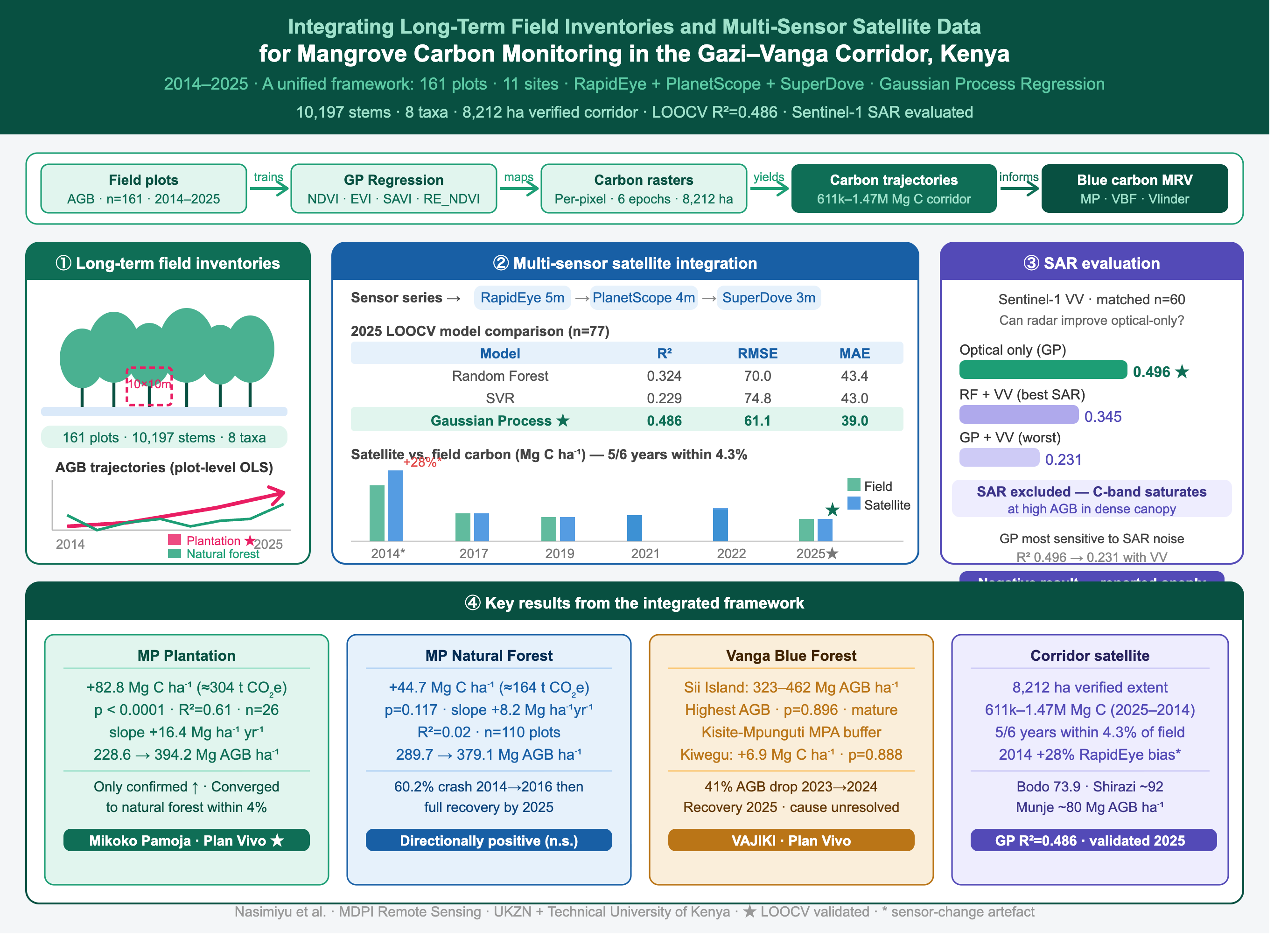
Community-based blue carbon projects generate long-term monitoring records that are rarely harmonized across sites or linked to validated satellite carbon frameworks, limiting landscape-scale assessment. This study integrated eleven years of permanent-plot inventories with multi-sensor satellite imagery across the 8,212 ha Gazi–Vanga mangrove corridor, Kenya. A unified species-specific allometric framework was applied to 10,197 trees across 161 plots (2014–2025), and Gaussian Process Regression was trained on RapidEye, PlanetScope, and SuperDove satellite imagery to produce corridor-wide carbon-density estimates. The restoration plantation at Gazi Bay showed the only statistically confirmed AGB increase (+16.4 Mg ha⁻¹ yr⁻¹; p < 0.0001; ≈304 t CO₂e ha⁻¹ over eleven years); other strata showed directionally positive but non-significant trends. Sii Island consistently maintained the highest biomass (324–462 Mg ha⁻¹), and first-inventory baselines were established for Bodo (73.9 ± 9.4 Mg ha⁻¹), Shirazi (79.7–104.3 Mg ha⁻¹), and Munje (59.9–100.2 Mg ha⁻¹). The satellite framework achieved R² = 0.486 (RMSE = 61.1 Mg C ha⁻¹; n = 77) and agreed closely with field means in five of six mapped years; a 28.1% divergence in 2014 coincided with a sensor transition. Sentinel-1 C-band SAR did not improve upon optical-only predictions. Community monitoring archives can be harmonized and integrated with Earth observation data to support cost-effective, landscape-scale blue carbon assessment in community-managed mangrove ecosystems.
Keywords:
mangroves
; blue carbon
; above-ground biomass
; community-based monitoring
; gaussian process regression
; remote sensing
; PlanetScope
; carbon accounting
; East Africa
1. Introduction
Mangrove forests are among the most carbon-dense and ecologically valuable ecosystems on Earth. Their carbon stocks, stored in above-ground biomass (AGB), below-ground roots, and deep sediment deposits, frequently exceed those of many tropical terrestrial forests and contribute significantly to long-term climate change mitigation [1,2]. Beyond carbon sequestration, mangroves provide a wide range of ecosystem services, including coastal protection, fisheries support, biodiversity conservation, and water purification, while sustaining the livelihoods of millions of coastal residents worldwide [3]. Despite their ecological and socioeconomic importance, global mangrove extent declined by approximately 5,000 km2 between 1996 and 2002 [4,5]. Recent global assessments indicate that many mangrove regions remain threatened by climate change, sea-level rise, and ongoing land-use pressures [6]. Along the Kenyan coastline, mangrove losses have been linked to timber harvesting, settlement expansion, and conversion to alternative land uses [7].
In response to these pressures, community-based blue carbon initiatives have emerged as a promising mechanism for linking mangrove conservation with climate-change mitigation and local livelihood enhancement. By generating carbon credits from mangrove conservation and restoration activities, such projects create financial incentives for ecosystem stewardship while supporting community development [8,9]. Demonstrating the effectiveness of these initiatives requires robust monitoring systems capable of quantifying carbon stocks and detecting changes through time across heterogeneous mangrove landscapes.
Kenya’s southern coast hosts two of the most influential community-managed blue carbon projects globally. Mikoko Pamoja (MP), established in Gazi Bay in 2013, was the first community-led mangrove carbon project to sell certified carbon credits under the Plan Vivo Standard [10]. Further south, Vanga Blue Forest (VBF) was validated under the Plan Vivo Standard in 2019 and became operational in 2020 under the VAJIKI Community Forest Association, covering a transboundary mangrove system extending from Shimoni, Kenya, towards northern Tanzania [11]. Together, these projects have generated more than a decade of field-based monitoring data through periodic forest inventories undertaken for monitoring, reporting, and verification (MRV) purposes. Such long-term datasets are rare for community-managed mangrove ecosystems and provide a valuable opportunity to evaluate carbon outcomes over time.
Remote sensing has become an increasingly important tool for mangrove monitoring and biomass estimation. At the global scale, the Global Mangrove Watch time series, derived from L-band SAR data across eleven epochs from 1996 to 2020, established a long-term baseline for tracking mangrove extent and change [12]. Along the Kenyan coast, previous studies have used optical imagery, vegetation indices, and field-validated allometric approaches to assess mangrove structural characteristics and estimate biomass [13,14]. More broadly, advances in Earth observation have enabled increasingly accurate estimation of forest biomass and carbon stocks using optical, radar, and LiDAR data, with the latest generation of PlanetScope SuperDove sensors providing enhanced spectral capabilities ,particularly the red-edge band, that substantially improve discrimination of mangrove structure compared to earlier four-band configurations [15]. However, biomass mapping remains subject to uncertainty arising from field measurements, allometric equations, sampling design, sensor characteristics, and statistical modelling approaches [16,17,18]. Remote sensing tools can help identify and efficiently quantify above-ground mangrove carbon stocks, yet accurately monitoring mangrove forests and their carbon storage capacity remains important for informing practitioners and policymakers interested in blue carbon conservation and crediting [19]. Maintaining strong links between field observations and satellite-derived products is therefore essential for reliable carbon assessment and reporting [20].
Despite the availability of long-term monitoring records, a significant knowledge gap remains. The monitoring archives of MP and VBF have been maintained independently and have never been harmonized and analyzed as a single monitoring record across the Gazi–Vanga mangrove corridor. Furthermore, while remote sensing has been applied to mangrove biomass estimation at individual sites and time periods, no study has continuously linked the long-term field inventories from both projects to a validated satellite carbon-monitoring framework. Consequently, long-term carbon trajectories across the corridor remain poorly understood, and the extent to which satellite observations can independently corroborate field-based carbon estimates has not been established.
Addressing this gap is important for both scientific and practical reasons. Harmonizing existing monitoring archives can recover valuable information on long-term biomass dynamics without the cost of establishing new monitoring networks. Remote sensing offers a transparent, replicable, and cost-effective approach for monitoring blue carbon ecosystems across large spatial and temporal scales [20].When combined with field observations, satellite monitoring provides a scalable means of assessing carbon density across heterogeneous mangrove landscapes, identifying areas with high restoration potential, detecting unusual biomass changes, and extending carbon estimates beyond sampled plots. Remote sensing is also well suited to tracking ecosystem dynamics and structural changes associated with carbon cycling that are difficult to capture through field measurements alone [21]. Despite the increasing importance of blue carbon ecosystems, remote-sensing studies of mangrove carbon stocks remain geographically uneven, with substantial knowledge gaps persisting across many major mangrove regions [19].
The novelty of this study lies in the integration of long-term community monitoring records and Earth observation data within a single analytical framework. To our knowledge, this is the first study to (i) harmonize more than a decade of monitoring data from two certified blue carbon projects in East Africa, (ii) analyze biomass dynamics at the scale of the Gazi–Vanga mangrove corridor, (iii) validate multi-sensor satellite-derived carbon estimates using the accumulated field archive, and (iv) extend carbon assessment to community-managed mangrove stands outside existing blue carbon project boundaries. To address these objectives, we first harmonize eleven years of Gazi Bay inventory data (2014–2025) and six years of VBF inventory data (2019–2025) using a unified species-specific allometric framework and evaluate temporal trends in AGB at the plot level. Second, we conduct a corridor-wide field inventory in 2025 covering both certified project areas and non-enrolled community forests to quantify contemporary carbon stocks across the Gazi–Vanga ecosystem. Third, we develop and validate a multi-sensor satellite monitoring framework using RapidEye, PlanetScope, and SuperDove imagery integrated through Gaussian Process Regression. Finally, we evaluate the contribution of Sentinel-1 C-band synthetic aperture radar (SAR) data to carbon-density prediction and assess its value for community-based mangrove carbon monitoring. Together, these analyses provide a field-validated assessment of mangrove carbon dynamics across one of the most important community-managed blue carbon landscapes in East Africa.
2. Materials and Methods
2.1. Study Area
The study spans the Gazi–Vanga mangrove corridor on Kenya’s southern coast, Kwale County (4°25′–4°40′S, 39°30′–39°35′E; Figure 1), part of a continuous mangrove system reaching across the border to Tanga, Tanzania. It includes two community-managed blue carbon sites, MP at Gazi Bay and VBF, about 60 km apart, plus the Bodo site under the Papariko project and the unaffiliated communities of Funzi, Shirazi and Munje.Gazi Bay, is approximately 50 km south of Mombasa in Msambweni District, supports a fishing population of 6,733 people in 1,081 households (115 persons/km2 over 58.3 km2; KNBS, 2019), with 1,000–1,600 mm annual rainfall, 19–34 °C temperatures, and freshwater input from the Mkurumudzi River, which rises in the Shimba Hills. Vanga, is approximately 100 km south of Mombasa in Lungalunga District near the Tanzanian border, spans the villages of Vanga, Jimbo, and Kiwegu (24,616 people, 4,563 households; 214 persons/km2 over 114.9 km2; [22,23]) with rainfall exceeding 1,000 mm/year, mean temperatures near 26 °C, and freshwater from the Umba River, originating in Tanzania’s Usambara Mountains [24,25].
Mikoko Pamoja, established in 2013 under the Plan Vivo Standard, was the world’s first community-based mangrove carbon project, covering 117 ha of natural forest and 10 ha of reforestation. VBF followed in 2019, also under Plan Vivo, at larger scale (450 ha natural forest, 5.25 ha plantation). Both generate revenue through avoided-deforestation and reforestation credits, reinvested in water, education, and health services [11,26].
Stands across the corridor are dominated by Rhizophora mucronata and Ceriops tagal, with Bruguiera gymnorrhiza, Sonneratia alba, Avicennia marina, Xylocarpus granatum, X. moluccensis, Lumnitzera racemosa, and Heritiera littoralis at varying densities [7,27]. Composition and structure differ markedly between natural and restored stands at Gazi, and between the managed Kiwegu network and Sii Island at Vanga, motivating a stratified design in which natural forest, plantation, and reference stands are monitored separately rather than pooled.
2.2. Data Collection
Plot monitoring was carried out using a 10 m × 10 m plot design (100 m2), consistent with the protocol of Kauffman and Donato [28] and previously applied at Gazi Bay and other coastal sites in Kenya and Tanzania [25,29]. At Gazi Bay, MP established and re-measured natural forest plots (MP1–MP10 , RMP1–RMP10; n = 20 in 2014 and 2017, reduced to n = 10 from 2020 onward following an internal protocol revision) and restoration plantation plots (PMP1–PMP10; n = 10 in 2017, n = 5 from 2022 onward). Plantation plots were randomly relocated at each survey round rather than permanently marked, because the spatial heterogeneity of restoration success across the plantation which varies substantially by treatment and microhabitat [30] makes fixed plots unrepresentative of the stratum as a whole. At Vanga, VAJIKI community maintained permanent plots across two strata: the Kiwegu village network (VPMP1–VPMP15 n = 11 per round) and the Sii Island stand (n = 4). A restoration site at Bazo and Makombe was established and first measured in 2024. In 2025, the lead author conducted a corridor-wide census re-surveying Gazi Bay and a subset of Vanga strata (Jimbo, Majoreni, and VBF Kiwegu), and extending coverage to community mangrove stands not previously inventoried: Bodo across seven village strata (n=10 plots total; plot allocation was constrained by tidal access windows across a spatially fragmented landscape), Shirazi (n=4), and Munje (n=6). This was designed to sample both certified project areas and adjacent non-enrolled stands, ensuring that the satellite model calibration dataset captured the full range of structural conditions present across the corridor, and to quantify above-ground carbon stock across the full Gazi–Vanga ecosystem. Table 1 summarizes the complete plot network by site, survey year, and stratum type and Figure 2 shows the field-satellite carbon monitoring workflow.
2.2.1. Mangrove Inventory and Plot Network
At each survey, all live mangrove stems with diameter at breast height (DBH) ≥2.5 cm were measured and identified to species within each 10 m × 10 m plot. DBH was recorded at 1.3 m above ground following standard forestry convention; for Rhizophora species, whose elevated prop roots make this point inaccessible, DBH was instead recorded 30 cm above the highest prop root, following Komiyama, et al. [31] and Kauffman and Donato [28]. The 2.5 cm minimum stem diameter aligns with the threshold used in prior Kenyan coastal mangrove inventories, including at Gazi Bay and across restoration sites in Kenya and Tanzania [29], ensuring comparability across survey years and sites. Across all years and sites, 10,197 individual tree records were compiled into a single species-coded dataset. In the Vanga 2021 and 2024 censuses, the field team used a measuring tape to record stem circumference directly rather than DBH; DBH was derived as circumference/π, an algebraically exact conversion that introduces no additional uncertainty beyond that of the original tape measurement (Table 1 and Table 4).
2.3. Data Analysis
2.3.1. Allometric Estimation and Field Carbon Calculation
Individual tree AGB was estimated using the pan-tropical mangrove allometric equation of Komiyama, Poungparn and Kato [31];
where D is DBH (cm) and ρ is species-specific wood density (g cm−3).
AGB = 0.251ρD2.46
Wood density values followed Komiyama, Poungparn and Kato [31] as shown in Table 2 from Njana, et al. [32] an East African determination, since Komiyama, Poungparn and Kato [31] measured the congener A. alba. Lumnitzera racemosa, present in <0.5% of records, used a flagged proxy value (0.700, cross-species hardwood-mangrove mean) given the absence of an East African-specific source; this affects a negligible AGB fraction and is noted as a limitation for future site-specific sampling for Gazi Bay species [33].
Plot-level AGB (Mg ha−1) was summed from individual trees within each 100 m2 plot and scaled to 1 ha. Stratum-level AGB per survey year is reported as the across-plot mean and median ± SE; single-plot strata lack an estimable SE and are flagged. Temporal trends in each of the four strata (Gazi Bay natural forest and plantation; Vanga Kiwegu network and Sii Island) were tested by OLS regression of plot-level AGB against survey date, rather than of stratum means, to preserve plot-to-plot variability and avoid artificially inflating precision. AGB was converted to carbon stock using the mangrove-specific carbon fraction of 0.50 (Kauffman and Donato, 2012; Eq 2) and to CO2-equivalent using the molecular-weight ratio 3.67 (Eq 3), consistent with MP and VBF Plan Vivo accounting.
Carbon = AGB × CF
CO2e = Carbon × 3.67
Inter-observer error is a relevant uncertainty source, as Gazi plots were measured across five epochs and Vanga plots across five to eight rounds, with the 2025 census conducted independently. Re-measurement by different observers typically introduces 3–8% systematic DBH error in mangroves [29,34], which propagates to ~12% error per stem and ~8–10% at plot level given the DBH2·46 scaling. This likely contributes to the large plot-to-plot SEs observed (20–84 Mg ha−1), alongside genuine ecological heterogeneity; disentangling the two would require replicate measurements by multiple observers, recommended as a future quality-assurance step [35] .
2.4. Satellite-Data Acquisition and Pre-Processing
Multi-sensor optical imagery was used to cover the Gazi–Vanga corridor across the full 2014–2025 study period, as no single sensor provided continuous coverage at high spatial resolution throughout the eleven-year monitoring window. RapidEye (5 m resolution, 5-band including red-edge) provided the 2014 baseline; PlanetScope (3–4 m, 4-band) covered 2017, 2019, and 2021; and SuperDove (3 m, 8-band including red-edge) covered 2022 and 2025. All imagery was atmospherically corrected to surface reflectance prior to index derivation, since raw sensor digital numbers are not directly comparable across dates or platforms and must first be converted to a physically meaningful reflectance scale. Four spectral vegetation indices were then computed from each annual satellite composite as candidate predictors of field-measured carbon density (AGB × 0.50 carbon fraction; Table 3, Equations 4–7). The indices were selected to capture complementary aspects of mangrove canopy condition: standard chlorophyll-related greenness (NDVI), atmospheric and soil-background noise correction with improved sensitivity in high-biomass closed canopy (EVI), soil background correction relevant to degraded stand edges (SAVI), and red-edge wavelength sensitivity in sensors that provide a red-edge band, specifically RapidEye and SuperDove (RE_NDVI). These indices were used to extend field-plot above-ground carbon estimates across the full 8,212 ha corridor extent, following a workflow of image preprocessing, vegetation index derivation, and integration with field-based ground truthing for carbon stock estimation.
2.5. Carbon Estimation and Trajectory
Earlier approaches to satellite-based mangrove carbon estimation typically relied on a single vegetation index regressed directly against field AGB. A multi-algorithm machine-learning approach was adopted instead, allowing multiple spectral predictors to be combined and compared formally rather than assuming a single index is sufficient. Because field sample sizes varied substantially across years (n = 15–77), only 2025 provided a sample large enough to support a statistically meaningful comparison of competing regression algorithms via leave-one-out cross-validation (LOOCV). LOOCV was chosen over held-out validation because it makes maximum use of the available sample, which is critical when n is small, and produces an unbiased estimate of generalization error without reducing the training set. Three algorithm classes were evaluated: Random Forest [37] , a non-parametric ensemble method robust to non-linearity and outliers; Support Vector Regression [38] which performs well in high-dimensional, small-sample settings; and Gaussian Process Regression [39], a kernel-based Bayesian method that provides probabilistic predictions and naturally quantifies predictive uncertainty. Predictor variables were standardized prior to model fitting using z-score normalization to minimize differences arising from varying index scales. The best-performing algorithm under LOOCV was adopted as the model class for all survey years and refit independently on each year’s own field plots before being applied pixel-by-pixel across the verified corridor boundary. Models for years other than 2025 were not independently cross-validated and their corridor-wide estimates are therefore treated as descriptive characterizations rather than validated predictions.
2.6. Sentinel-1 SAR Evaluation
Sentinel-1 VV backscatter was evaluated as an additional predictor for 2025 to test whether radar-derived structural information could improve upon optical indices alone. SAR backscatter is sensitive to canopy geometry and woody biomass at low-to-moderate density but is predicted to saturate at higher biomass levels in dense canopy forest, because the radar signal cannot penetrate to the lower canopy and woody stems [18].Because SAR coverage was available for only a subset of 2025 plots, the evaluation was restricted to a matched sample of n = 60 plots with both optical and SAR data, allowing a like-for-like comparison against the optical-only baseline. All three algorithms (Random Forest, Support Vector Regression, Gaussian Process Regression) were tested on this matched sample under four feature sets: optical indices alone, optical plus VV in decibel scale, optical plus VV in linear power scale, and optical plus both VV representations combined. SAR was retained in the final model only if the best SAR-inclusive combination, for any algorithm, improved on the optical-only baseline; if not, SAR was excluded and the negative result reported as a methodologically useful finding for community monitoring programmes considering radar integration (Section 3.4).
2.7. Corridor Area Verification
The corridor-wide study area boundary was derived from an existing mangrove extent shapefile comprising 36 polygon features. Because several of the largest features overlapped one another, the naive sum of individual polygon areas overstated the true extent; the non-overlapping area was therefore established independently via vector-geometry union calculation in ArcGIS software and cross-checked against raster-pixel masking for each of the six satellite epochs, both converging on 8,212 ha. This verified value, rather than the naive polygon sum, is used for all corridor-wide area and total-carbon figures in this study. The audit was performed before model application, so that the same boundary was applied consistently across all years and could not itself introduce apparent differences between years.
2.8. Field–Satellite Comparison (Plausibility Check)
For each year, the satellite-derived corridor-wide mean carbon density was compared against that year’s field-plot mean, extrapolated to the 8,212-ha study area, as a plausibility check. This comparison is explicitly not a validation: extrapolating 15–77 plot means carries substantial uncertainty of its own (field-plot standard deviations of 62–86 Mg C ha−1 across years), and the satellite model carries its own prediction uncertainty, quantified by the leave-one-out RMSE reported in Section 3.3. Both sides of the comparison therefore carry errors of comparable magnitude, and close agreement should be read as mutual plausibility support rather than independent ground-truthing of either estimate.
3. Results
3.1. Harmonized AGB Trajectories and Carbon Stocks: Gazi Bay and Vanga Blue Forest
Across the monitored strata, above-ground biomass trajectories ranged from stable and high-biomass at Sii Island to strongly recovering at the Gazi Bay restoration plantation. Statistically significant biomass accumulation was detected only in the Gazi Bay restoration plantation, whereas the adjacent natural forest, both Vanga strata, and the satellite-derived corridor-wide carbon-density series exhibited directionally positive but statistically non-significant trends, reflecting substantial interannual variability and plot-to-plot heterogeneity at current sample sizes. The sections below describe each stratum in turn before the corridor-wide 2025 baselines and the satellite carbon framework are presented.
The final harmonized dataset comprised 10,197 individually measured stems across 161 plots, 11 sites, and six survey epochs spanning 2014 to 2025, representing eight canonical mangrove taxa (Table 1). Four strata in Gazi Bay natural forest, Gazi Bay restoration plantation, Vanga Kiwegu network, and Vanga Sii Island contributed multi-year trajectory data. Seven additional strata contributed 2025 baseline measurements only. The Gazi Bay natural forest showed marked AGB variation across the monitoring period (Table 4). Mean AGB was 289.7 Mg ha−1 (median 257.5; n = 14 plots) at the 2014 baseline, fell to 115.3 Mg ha−1 (median 75.3; n=10) by 2016, a reduction of 60.2% that is the largest single-epoch decline observed in any stratum and then rose progressively through three quarterly rounds in 2017 (mean 146.5, 208.6, and 223.0 Mg ha−1) and continued increasing, with a secondary dip to 190.1 Mg ha−1 in April 2021, to reach a peak of 379.1 Mg ha−1 (median 304.8; n=10) in 2025. Despite this visually compelling recovery trajectory, plot-level ordinary least-squares regression of AGB against survey date across all rounds revealed no statistically significant trend (slope = +8.2 Mg ha−1 yr−1, p=0.117, R2=0.02).The non-significance reflects the substantial and real plot-to-plot variability within each survey round (standard errors of 20–84 Mg ha−1) rather than an absence of biological change, and should be understood as a statement about statistical certainty at current sample sizes rather than about the underlying ecological trajectory.

Table 4.
Above-ground biomass (AGB) at Gazi Bay, Kwale County, Kenya, by survey year: (a) natural forest stratum, permanent plots (MP1–MP10 / RMP1–RMP10).
Table 4.
Above-ground biomass (AGB) at Gazi Bay, Kwale County, Kenya, by survey year: (a) natural forest stratum, permanent plots (MP1–MP10 / RMP1–RMP10).
| Year | n | Mean (Mg/ha) | Median (Mg/ha) |
| 2014 | 14 | 289.7 | 257.5 |
| 2016 | 10 | 115.3 | 75.3 |
| 2017-04 | 10 | 146.5 | 142.6 |
| 2017-08 | 10 | 208.6 | 118.7 |
| 2017-11 | 20 | 223.0 | 187.7 |
| 2020 | 10 | 269.6 | 269.3 |
| 2021-04 | 10 | 190.1 | 166.0 |
| 2022-05 | 15 | 234.5 | 218.7 |
| 2022-09 | 10 | 243.5 | 128.4 |
| 2025 | 10 | 379.1 | 304.8 |
The restoration plantation showed a contrasting pattern (Table 5). Mean AGB was 228.6 Mg ha−1 (median 212.5; n=6 randomly relocated plots) at the 2014 baseline, was effectively unchanged in November 2017 (199.3 Mg ha−1; n=10), and then rose to 317.7 Mg ha−1 in September 2022 (n=5) and 394.2 Mg ha−1 (median 391.9; n=5) in 2025, an endpoint-to-endpoint gain of 165.6 Mg ha−1 over eleven years. Plot-level regression across the three available epochs (2014, 2022, 2025) detected a statistically significant positive trend (slope = +16.4 Mg ha−1 yr−1, p < 0.0001, R2=0.61), making the restoration plantation the only one of the four main strata in this study with a statistically confirmed AGB increase over time. By 2025, the mean AGB of the plantation (394.2 Mg ha−1) and natural forest (379.1 Mg ha−1) had converged to within 4%.
3.1.2. Vanga Blue Forest: Kiwegu Network and Sii Island
The Kiwegu village network showed a non-monotonic pattern across five survey epochs (Table 6). Mean AGB rose from 103.1 Mg ha−1 at the 2019 baseline (n=11 plots) to a peak of 123.9 Mg ha−1 in May 2023, fell sharply to 72.9 Mg ha−1 (median 67.0) in May 2024, a reduction of 41.2% from the preceding year and recovered to 116.8 Mg ha−1 (median 126.2) in 2025. Plot count was identical at n=11 in each of the 2023, 2024, and 2025 rounds. Despite this pronounced interannual variation, plot-level ordinary least-squares regression across the four complete rounds found no statistically significant temporal trend (slope = −0.9 Mg ha−1 yr−1, p = 0.888, R2 < 0.01). The Sii Island stratum showed the highest mean AGB of any stratum in this study at every survey round, ranging from 323.6 to 462.2 Mg ha−1 across eight rounds spanning 2019 to 2025 (Table 7). Plot-level regression likewise found no statistically significant trend across this period (p = 0.896).
3.1.3. Carbon Stock Conversion and Net Gains
At the most recent survey, every stratum’s estimated above-ground carbon stock exceeded its baseline value (Figure 3). Gazi Bay restoration plantation showed the largest absolute gain: 82.8 Mg C ha−1 (approximately 304 t CO2e ha−1) from 2014 to 2025, the only endpoint-to-endpoint gain that was also confirmed by a statistically significant temporal trend (p<0.0001). The Gazi Bay natural forest gained 44.7 Mg C ha−1 (approximately 164 t CO2e ha−1) over the same period; the trend underlying this gain was not statistically significant (p=0.117). At Vanga, the Kiwegu network gained 6.9 Mg C ha−1 (approximately 25 t CO2e ha−1) and Sii Island gained 2.0 Mg C ha−1 (approximately 7 t CO2e ha−1) from 2019 to 2025; neither trend was statistically significant (p = 0.888 and p = 0.896, respectively). The four strata’s net carbon gains are shown in Figure 3b alongside their trajectories over time.
3.2. Corridor-Wide Carbon Stock: Enrolled and Non-Enrolled Stands
Of the 161 plots measured in the 2025 corridor-wide census, 30 were located at community mangrove stands without a prior structural inventory covering both non-enrolled communities and additional Vanga strata reported here as first-time carbon stock measurements for those areas (Table 8). The Bodo area-wide mean AGB, pooling all seven village strata (n = 10 plots), was 73.9 ± 9.4 Mg ha−1. Within-area variation was substantial: individual village stratum means ranged from 13.7 Mg ha−1 at Uwanja wa Shule to 102.8 Mg ha−1 at Chupaani. At Shirazi, the two sampled villages showed means of 79.7 ± 7.9 Mg ha−1 (KwaEdimundI) and 104.3 ± 24.9 Mg ha−1 (Kwaghafuru). At Munje, means were 59.9 ± 18.8 Mg ha−1 (Kwa makata; n = 4) and 100.2 ± 32.0 Mg ha−1 (Mkawatsi; n = 2). These values are broadly comparable to the Bodo area mean and to the lower end of the Vanga Kiwegu network range (103.1–123.9 Mg ha−1 across non-anomalous rounds). Among the additional 2025 Vanga strata, Majoreni had the lowest mean AGB (39.8 ± 13.3 Mg ha−1; n = 6), followed by Jimbo (57.9 ± 11.3 Mg ha−1; n = 10) and the separately recorded VBF Kiwegu stratum (78.8 ± 20.2 Mg ha−1; n = 9). When these three strata were combined with the 2025 Sii Island survey (n = 6), the VBF-wide pooled mean was 116.5 ± 23.8 Mg ha−1 across 31 plots.
3.3. Satellite Carbon Monitoring Framework
Gaussian Process Regression outperformed Random Forest and Support Vector Regression under leave-one-out cross-validation for 2025 (n = 77; Table 9) and was applied as the model class across the full time series. The 2025 Gaussian Process Regression model explained 48.6% of variance in plot-level carbon density (R2 = 0.486, RMSE = 61.1 Mg C ha−1, n = 77; Figure 4, right panel). Satellite-derived corridor-wide mean carbon density ranged from 74.5 Mg C ha−1 in 2025 to 178.6 Mg C ha−1 in 2014, corresponding to total carbon stocks of 611,659 and 1,466,389 Mg C, respectively, across the 8,212-ha corridor extent (Table 10). In five of six years (2017, 2019, 2021, 2022, 2025), satellite-derived mean carbon density was within 4.3% of the corresponding field-plot mean, with differences ranging from −4.3% to −0.1% (mean absolute difference 1.9%; Figure 4, left panel). The largest divergence occurred in 2014, where the satellite estimate (178.6 Mg C ha−1) exceeded the field-plot mean (139.4 ± 70.2 Mg C ha−1) by 28.1%; this year had the smallest field sample (n = 16) and was the only epoch using RapidEye imagery.
Corridor-wide spatial distributions of satellite-derived carbon density are shown in Figure 5, Figure 6, Figure 7 and Figure 8 for each year. The maps reveal spatially heterogeneous carbon density within the corridor, consistent with the aggregate means in Table 10. The spatial footprint of high carbon density is largest in 2025 and smallest in 2014. The 2014 map (RapidEye) shows a visually distinct pattern from the five PlanetScope/SuperDove years, with higher predicted density across much of the corridor interior, consistent with the sensor-related divergence. For 2025 (Figure 8) stands in Gazi blue carbon project, Sii Island, creek margins, highest density, as verified in section 3.3.
3.4. Sentinel-1 SAR Evaluation
Optical indices alone achieved the highest performance of any combination tested (R2 = 0.496, Gaussian Process Regression). Every SAR-inclusive combination performed worse than this optical-only baseline, regardless of algorithm or VV representation. Gaussian Process Regression, the best-performing algorithm on optical indices alone, showed the largest decline in performance when SAR was added (R2 falling from 0.496 to 0.231–0.299 across the three SAR-inclusive feature sets), a substantially steeper drop than Random Forest (0.349 to 0.336–0.345) or Support Vector Regression (0.303 to 0.285–0.300). Random Forest with VV in linear power scale was therefore the best-performing SAR-inclusive combination overall (R2 = 0.345), but this result remained below the optical-only baseline achieved by Gaussian Process Regression. SAR was excluded from the final model on this basis.
Table 11.
Leave-one-out cross-validation comparison of optical-only and SAR-inclusive feature sets across three machine learning algorithms, 2025 matched sample (n = 60).
Table 11.
Leave-one-out cross-validation comparison of optical-only and SAR-inclusive feature sets across three machine learning algorithms, 2025 matched sample (n = 60).
| Feature set | Model | R2 | RMSE (Mg C ha−1) | MAE (Mg C ha−1) |
|---|---|---|---|---|
| Optical only (n=60 matched sample) | Gaussian Process Regression | 0.496 | 61.6 | 38.8 |
| Optical only (n=60 matched sample) | Random Forest | 0.349 | 70.0 | 42.5 |
| Optical only (n=60 matched sample) | Support Vector Regression | 0.303 | 72.5 | 42.4 |
| Optical + VV (dB) | Random Forest | 0.336 | 70.7 | 42.3 |
| Optical + VV (dB) | Support Vector Regression | 0.300 | 72.6 | 40.8 |
| Optical + VV (dB) | Gaussian Process Regression | 0.299 | 72.7 | 44.1 |
| Optical + VV (linear power) | Random Forest | 0.345 | 70.3 | 42.3 |
| Optical + VV (linear power) | Support Vector Regression | 0.296 | 72.8 | 41.0 |
| Optical + VV (linear power) | Gaussian Process Regression | 0.231 | 76.1 | 52.5 |
| Optical + VV (dB and power) | Random Forest | 0.339 | 70.5 | 42.2 |
| Optical + VV (dB and power) | Support Vector Regression | 0.285 | 73.4 | 41.0 |
| Optical + VV (dB and power) | Gaussian Process Regression | 0.283 | 73.5 | 50.6 |
4. Discussion
4.1. Harmonized AGB Trajectories and Carbon Stock Change
4.1.1. Gazi Bay: Restoration Plantation and Natural Forest
The principal finding of this study is that eleven years of community-monitored field data, harmonized using a single species-specific allometric framework, demonstrate a statistically significant increase in AGB within the Gazi Bay restoration plantation (+16.4 Mg ha−1 yr−1, p < 0.0001). This was the only statistically significant trend detected among the four principal strata examined. In contrast, the adjacent natural forest, both Vanga strata, and the satellite-derived corridor-wide carbon-density estimates exhibited directionally positive trajectories that were not statistically significant at the current sample sizes. The observed rate of 16.4 Mg ha−1 yr−1 substantially exceeds the accumulation rate of 8.9 Mg ha−1 yr−1 recorded for the same Rhizophora mucronata plantation stand at Gazi Bay when it was 12 years old [40],consistent with continued and accelerating biomass accumulation in a maturing stand well beyond the period covered by that earlier structural assessment. This trajectory also falls within the broader range of biomass accumulation rates documented for tropical mangrove restoration plantations globally, which vary widely depending on stand age, species, and site conditions [41]
Several complementary ecological processes may contribute to the plantation’s confirmed increase. Continued growth of the original Rhizophora mucronata cohort, whose survival varies according to microsite conditions and protection measures [30], is likely accompanied by natural recruitment of additional mangrove species into the stand, consistent with the broader species assemblages reported across the Gazi–Vanga corridor [27].Seedling establishment and forest expansion in mangrove ecosystems are strongly influenced by hydrodynamic thresholds that regulate propagule retention and survival [42]. Moreover, studies have shown that natural recruitment can become a major driver of biomass recovery in restored mangroves once suitable hydrological conditions are re-established, complementing or even exceeding the contribution of active planting efforts [41,43].
The convergence of plantation and natural-forest mean AGB to within approximately 4% by 2025 (394.2 versus 379.1 Mg ha−1) represents a notable and management-relevant outcome. This result suggests that the restored stand has attained an above-ground carbon storage level comparable to that of the adjacent reference forest. However, this similarity applies only to AGB and should not be interpreted as evidence of complete ecological equivalence. Important ecosystem attributes including species composition, structural complexity, faunal assemblages, nutrient dynamics, and soil-carbon development, may continue to differ substantially between restored and natural forests, even where above-ground carbon stocks converge [43,44].
The natural forest trajectory includes a pronounced decline from 289.7 Mg ha−1 at the 2014 baseline to 115.3 Mg ha−1 in 2016, representing a 60.2% reduction within a single monitoring interval and the largest decline observed in any stratum in this study (Section 3.1). Biomass subsequently increased over the following decade. As with the later decline observed within the Kiwegu network (Section 4.1.2), the available plot data do not permit attribution of this reduction to a specific cause. Potential drivers include storm impacts, extreme tidal events, disease, localized mortality, or other disturbance processes. Nevertheless, the observed decline and subsequent recovery are consistent with growing evidence that mangrove ecosystems often experience episodic disturbance–recovery dynamics rather than continuous monotonic change. Mangrove carbon stocks may decline sharply following disturbance events but recover substantially over subsequent years, depending on disturbance severity, stand age, and hydrological conditions [45]. Interpreting any single survey year in isolation therefore risks mistaking a transient disturbance signal for a long-term change in ecosystem carbon storage.
The non-significant trend observed in the natural forest (p = 0.117) likely reflects substantial within-stratum variability relative to the available sample size. Standard errors ranged from approximately 20 to 84 Mg ha−1 among survey rounds, indicating considerable plot-to-plot heterogeneity. Such variability is characteristic of naturally regenerating and structurally complex forest systems, where localized mortality, recruitment, and growth processes can dominate short-term temporal variation [46,47]. Consequently, the absence of statistical significance should not be interpreted as evidence of ecological stability or lack of biomass change. Rather, it reflects the current statistical power of the monitoring design. Expansion of the plot network or continued long-term monitoring would improve the ability to distinguish directional ecological change from background spatial variability.
4.1.2. Disturbance and Recovery in the Kiwegu Network
The 41% decline in AGB observed within the Kiwegu village network between May 2023 and May 2024, followed by recovery to near-2023 levels in 2025, represents the most ecologically significant anomaly in the dataset. This pattern is inconsistent with gradual degradation and instead suggests an acute disturbance event followed by rapid recovery. Although the underlying driver cannot be identified from the plot data alone, potential causes include storm impacts, extreme tidal inundation, disease outbreaks, or localized mortality events. The subsequent recovery indicates that the ecological conditions necessary for regeneration remained largely intact. Mangrove establishment and post-disturbance recovery are strongly influenced by tidal hydrodynamics, sediment stability, and propagule dispersal processes, which regulate seedling recruitment and survival [42,48]. Recent studies demonstrate that hydrological rehabilitation and associated community-based restoration actions can recover most of the ecosystem carbon stocks lost after disturbance, particularly when tidal connectivity and sediment conditions remain favorable, highlighting the inherent resilience of these ecosystems [49] Such disturbance-recovery dynamics reinforce the importance of long-term monitoring, as interpretations based on a single survey year may misrepresent temporary declines as persistent losses in ecosystem carbon stocks.
4.1.3. Sii Island as a High-Carbon Reference Stand
Sii Island consistently exhibited the highest above ground carbon of any stratum throughout the monitoring period, ranging from 323.6 to 462.2 Mg ha−1 across the eight survey rounds. These values substantially exceeded those recorded in the Gazi Bay natural forest and the non-enrolled community-managed stands and fall within the upper range of biomass reported for mangrove ecosystems globally [50].Despite its high biomass, no significant temporal trend was detected (p = 0.896), indicating remarkable stability over the six-year observation period. The absence of a significant trend is consistent with a mature stand approaching structural equilibrium, where biomass gains through tree growth are broadly balanced by mortality and natural turnover; biomass and carbon storage in mature mangroves exhibit relatively static and stable characteristics at interannual scales compared to more dynamic ecosystem processes such as gross primary production (Adame et al., 2024). Under such conditions, net changes in AGB between survey rounds are expected to be small relative to the spatial variability captured by the current sampling design, a pattern consistently observed in old-growth mangrove stands where forest age is the primary determinant of biomass accumulation and where mature stands show limited further change [51,52]. The long-term stability observed at Sii Island therefore suggests the presence of a persistent carbon reservoir that continues to maintain high biomass while exhibiting relatively limited interannual variation.
Sii Island’s location within the buffer zone of the Kisite–Mpunguti Marine Protected Area (Section 2.1) may contribute to its sustained high biomass by limiting anthropogenic disturbance and supporting natural ecosystem processes. Beyond carbon storage, high-biomass mangrove forests provide a wide range of ecosystem services, including shoreline stabilization, coastal protection, nursery habitat for fisheries, biodiversity conservation, and support for local livelihoods [53,54].Recent global assessments further emphasize the importance of intact mangrove ecosystems for climate regulation, coastal resilience, and biodiversity conservation. These broader ecological functions suggest that the value of Sii Island extends well beyond its carbon stock alone and reinforce its importance as a conservation asset within the Gazi–Vanga corridor [55].
From a monitoring perspective, the high and stable above ground carbon observed at Sii Island makes it a valuable reference site for future satellite-based model calibration and validation. As one of the highest-biomass stands within the corridor, it represents the upper range of carbon densities that remote-sensing models must predict. Dense mangrove forests are particularly useful for evaluating potential optical-sensor saturation effects, a well-recognized limitation of biomass estimation in high-carbon ecosystems. Such stands therefore provide an important benchmark for assessing uncertainty and prediction bias in satellite-derived biomass and carbon-density products [56,57].
4.2. Corridor-Wide Carbon Stocks
The 2025 baseline carbon stocks recorded at Bodo (73.9 ± 9.4 Mg ha−1), Shirazi (79.7–104.3 Mg ha−1), and Munje (59.9–100.2 Mg ha−1) occupy an intermediate position between the lowest-biomass Vanga stratum (Majoreni, 39.8 Mg ha−1) and the high-biomass reference stands of Gazi Bay and Sii Island. These values are broadly comparable to the lower end of the Kiwegu village-network range (103.1–123.9 Mg ha−1 across non-anomalous survey rounds) and fall within the range previously reported for community-managed mangrove forests along the Kenyan coast.[29], these results indicate that substantial carbon stocks are present across the wider Gazi–Vanga corridor, although considerable variation exists among sites and management contexts.
The nearly sevenfold variation observed among Bodo strata (13.7–102.8 Mg ha−1) highlights pronounced spatial heterogeneity in above-ground carbon stocks and has important implications for project baseline development. In particular, the exceptionally low biomass recorded at Uwanja wa Shule (13.7 Mg ha−1) may reflect a relatively young regenerating stand, a previously disturbed area, or a site with a history of clearance. Regardless of the underlying cause, this contrast demonstrates that neighboring mangrove stands can differ substantially in carbon-storage capacity despite occurring within the same community landscape. This heterogeneity presents a challenge for blue-carbon accounting. Aggregating all village strata into a single mean value (73.9 Mg ha−1) simplifies reporting but may obscure ecologically meaningful differences among stands. Where carbon stocks vary substantially between strata, the use of a single area-wide baseline may influence estimates of additionality and carbon benefits, particularly if future restoration or conservation interventions are concentrated within specific portions of the landscape rather than applied uniformly across the site [58,59].Consequently, stratified approaches to baseline development may provide a more accurate representation of carbon dynamics and project outcomes in heterogeneous mangrove systems.
For Shirazi and Munje, the observed carbon stocks are comparable to those of the less-degraded Bodo strata and suggest that ecological conditions are sufficient to support future blue-carbon initiatives. The main constraints to project development therefore appear likely to be institutional rather than biophysical. Successful blue-carbon projects require not only adequate carbon stocks but also long-term governance structures, community participation, monitoring capacity, and transparent benefit-sharing mechanisms [60,61]. The experiences of Mikoko Pamoja and Vanga Blue Forest demonstrate that the establishment of community forest associations, sustained local engagement, and robust monitoring frameworks are critical prerequisites for project registration and long-term success [10,62]. Consequently, future expansion of blue-carbon initiatives within the corridor may depend as much on strengthening local institutional capacity as on the carbon sequestration potential of the mangrove resource itself.
4.3. Satellite Carbon Monitoring Framework
The 2025 Gaussian Process Regression model explained 48.6% of variance in plot-level carbon density (R2 = 0.486, RMSE = 61.1 Mg C ha−1, n = 77). This level of performance is broadly consistent with that reported in optical remote-sensing studies of mangrove biomass and carbon estimation, where prediction accuracy is often constrained by species heterogeneity, structural complexity, and environmental variability within mangrove ecosystems [63,64] model therefore provides a useful basis for corridor-scale carbon monitoring while acknowledging that a substantial proportion of local-scale variation remains unexplained. The moderate explanatory power is also consistent with the well-documented saturation of optical vegetation indices in dense mangrove canopies. As AGB increases, spectral responses in visible and near-infrared wavelengths become progressively less sensitive to additional biomass accumulation, reducing the ability of optical sensors to discriminate among high-biomass stands [18,65].This limitation may explain why Sii Island, the highest-AGB stratum in the monitoring network, is likely to be underestimated by the satellite model despite being correctly identified as a high-carbon-density area within the corridor-wide maps. Consequently, the mapped outputs should be interpreted primarily as indicators of relative spatial patterns in carbon density rather than precise estimates at the upper end of the biomass gradient.
Despite these limitations, the framework produced corridor-wide carbon-density estimates that were generally consistent with independent field measurements. In five of the six analyzed years, the satellite-derived mean carbon density differed by less than 4.3% from the corresponding field-plot mean (Section 3.3). The notable exception was 2014, when the satellite-derived estimate differed from the field-based mean by 28.1%, coinciding with the smallest field sample size (n = 16) and the only year in which RapidEye imagery was used. The sensor systems differ in spectral-band configuration, spectral response functions, radiometric characteristics, spatial resolution, and image-processing workflows, all of which are known to influence vegetation indices and biomass predictions derived from optical remote-sensing data. Baloloy, et al. [66] directly demonstrated that RapidEye, PlanetScope, and Sentinel-2 produce measurably different biomass prediction performance for mangroves, while radiometric consistency between successive PlanetScope generations is a recognized challenge in multi-temporal analyses [67].
As a result, the apparent difference between the 2014 estimate and subsequent years cannot currently be separated confidently from potential sensor-related bias. Before interpreting the 2014–2025 trajectory as evidence of ecological change, future work should quantify cross-sensor effects through formal harmonization procedures, such as extracting RapidEye reflectance values at the 2014 field-plot locations and comparing them with a contemporaneous reference sensor. Such harmonization approaches are increasingly recommended for long-term monitoring frameworks that combine data from multiple sensor [12,20].
The corridor-wide spatial patterns reported in Section 3.3 are broadly consistent with the aggregate annual means presented in Table 5 and with the sensor-related divergence discussed above. However, site-specific spatial interpretations have been deliberately avoided because these observations have not been independently validated against the source raster outputs. This cautious approach is consistent with broader recommendations from the remote-sensing biomass literature, which emphasize rigorous model validation, uncertainty assessment, and careful interpretation of spatial products derived from satellite-based biomass and carbon estimates [18,19].
4.4. SAR Evaluation and Implications
The inclusion of Sentinel-1 VV backscatter did not improve carbon-density prediction relative to optical predictors alone. Using the matched dataset (n = 60), the best SAR-inclusive model achieved an R2 of 0.345, compared with an R2 of 0.496 for the optical-only model (Section 3.4). This finding suggests that optical vegetation indices captured a greater proportion of the variation in mangrove carbon density than the Sentinel-1 VV signal within the Gazi–Vanga corridor. Similar limitations have been reported in forest and mangrove biomass studies, where the sensitivity of remotely sensed predictors, including radar backscatter, may decline at higher biomass levels because of signal saturation and increasing canopy complexity [18,65,68].
The effect of SAR integration was not uniform across modelling approaches. Gaussian Process Regression (GPR), which produced the highest predictive accuracy using optical variables alone, exhibited the largest decline in performance following the inclusion of VV backscatter, with R2 decreasing from 0.496 to 0.231–0.299 depending on the VV representation used. In contrast, Random Forest showed only a marginal reduction (0.349 to 0.336–0.345), while Support Vector Regression decreased from 0.303 to 0.285–0.300. A plausible explanation lies in the differing characteristics of the modelling algorithms. GPR is particularly well suited to small ecological datasets because it models smooth, nonlinear relationships through kernel-based covariance functions without requiring large training samples and has been demonstrated to be among the most competitive machine learning algorithms for predicting vegetation biophysical variables precisely when sample sizes are small [39,69]. The superior performance of the optical-only GPR model therefore suggests that variation in carbon density across the corridor was effectively captured by the optical predictors alone, and that adding VV backscatter increased model complexity without improving predictive accuracy.
By comparison, Random Forest and Support Vector Regression appeared more robust to the inclusion of VV backscatter. Random Forest reduces the influence of less informative predictors through recursive tree construction, while Support Vector Regression constrains model fitting through regularization and support-vector selection [37,38]. Consequently, the effect of SAR integration depended not only on the characteristics of the radar signal but also on how individual modelling frameworks utilized the available predictor set. These results suggest that SAR-inclusion decisions for small-sample community monitoring programmes should be tested independently for each candidate algorithm rather than assumed to generalize across model classes.
Taken together, the optical predictors contained most of the information required to model carbon-density variation across the Gazi–Vanga corridor. Increasing the number of input datasets did not improve predictive performance, underscoring that for community-scale mangrove carbon monitoring, model performance depends on both the relevance of predictor variables and the modelling approach used. Improvements in field sampling density, temporal consistency, and optical-model calibration are therefore likely to yield greater gains in prediction accuracy than the inclusion of Sentinel-1 VV backscatter.
Future work should investigate L-band SAR missions such as ALOS-4 PALSAR-3, GEDI-derived canopy height and structure metrics, or airborne LiDAR can overcome the saturation limitations observed with Sentinel-1 C-band data in this study. L-band radar penetrates more deeply into dense mangrove canopy than C-band and saturates at higher biomass levels, making it a theoretically more promising complement to optical monitoring in high-biomass settings such as the Gazi Bay natural forest and Sii Island stands.
4.5. Strengths and Limitations
A major strength of this study is the harmonization of more than a decade of permanent-plot monitoring data from two certified blue carbon projects using a consistent species-specific allometric framework [31]. This provided a rare opportunity to examine long-term AGB dynamics across the Gazi–Vanga mangrove corridor using a common analytical approach. The 2025 inventory (n = 77 plots) represents the largest single-year field survey conducted across the corridor and provided the calibration dataset for the satellite carbon-monitoring framework. The use of plot-level data for formal statistical testing of biomass change, rather than reliance on stratum means, allowed robust distinction of significant trends from natural variability and reduced the risk of overstating conclusions, an approach consistent with current best practice for error-propagation-aware biomass estimation [70].
Several limitations should be considered when interpreting the results. First, the satellite-derived carbon-density estimates were formally validated only for 2025. Consequently, the 2014–2022 maps should be interpreted as descriptive representations of spatial carbon patterns rather than fully validated carbon products. Interpretation of temporal trends is further complicated by the unresolved sensor difference between the 2014 RapidEye imagery and the PlanetScope/SuperDove imagery used in subsequent years (Section 4.3). More broadly, uncertainty in satellite-based biomass mapping can accumulate from multiple sources, including field measurements, allometric equations, sampling design, and remote-sensing model error, with sampling error often identified as the dominant contributor at the site level [17,70]. Transparency about these uncertainty sources is essential for reliable carbon monitoring and verification frameworks [71].
Finally, the random-relocation plot design used in the Gazi Bay plantation was suitable for estimating stand-level biomass but did not allow repeated measurement of individual trees. As a result, while the observed increase in plantation AGB is statistically supported, the relative contributions of tree growth, recruitment, and mortality cannot be determined from the available data. Permanent plot networks with individually tagged stems would resolve this limitation and are recommended as a priority for any future expansion of the monitoring programme, as individual-tree tracking is increasingly recognized as the irreplaceable ground-level foundation for detecting biomass change over time [72,73].
5. Conclusions
This study combined long-term community monitoring data and satellite observations to assess AGB and carbon dynamics across the Gazi–Vanga mangrove corridor. Using a harmonized allometric framework, the analysis showed that the Gazi Bay restoration plantation was the only stratum with a statistically significant increase in AGB over the monitoring period (+16.4 Mg ha−1 yr−1, p < 0.0001). In contrast, the natural forest and Vanga strata showed generally positive but non-significant trends, reflecting substantial spatial variability among plots. The 2025 field inventory established new carbon baselines for Bodo, Shirazi, and Munje and confirmed Sii Island as the highest-carbon stand within the corridor. The large variation observed among sites highlights the importance of stratified carbon assessments and demonstrates that substantial carbon stocks extend beyond the currently certified blue carbon project areas.
The satellite monitoring framework successfully mapped carbon density across the corridor and produced estimates that closely matched field measurements in most years. However, differences between the 2014 RapidEye imagery and the PlanetScope/SuperDove imagery used in later years introduce uncertainty that currently limits interpretation of long-term satellite trends. The satellite products should therefore be viewed as a valuable complement to field monitoring rather than a replacement for it. The inclusion of Sentinel-1 VV backscatter did not improve model performance relative to optical predictors alone. The best-performing model was an optical-only Gaussian Process Regression model, indicating that freely available optical imagery can provide a practical and cost-effective basis for corridor-scale mangrove carbon monitoring in this region.
Overall, the study demonstrates that community-based field monitoring, combined with satellite observations and robust statistical analysis, can support landscape-scale carbon assessment in mangrove ecosystems. The framework developed here provides a practical approach for expanding carbon monitoring across community-managed blue carbon initiatives along the East African coast. The proposed framework is scalable and transferable beyond this corridor, offering an integrated approach for combining community-based field monitoring with Earth observation to support long-term blue carbon monitoring, carbon-credit verification, and mangrove conservation across tropical coastal ecosystems.
Supplementary Materials
The following supporting information can be downloaded at the website of this paper posted on Preprints.org, Figure S1: title;.
Author Contributions
Conceptualization, B.L.N.; methodology, B.L.N.; software, B.L.N.; formal analysis, B.L.N.; investigation, B.L.N.; data curation, B.L.N.; writing—original draft preparation, B.L.N.; writing—review and editing, B.L.N.; visualization, B.L.N.; project administration, B.L.N.; resources, R.N.M. (satellite imagery), R.N.M. (revising); supervision, M.G, R.N.M. All authors have read and agreed to the published version of the manuscript.
Funding
This research received no external funding.
Data Availability Statement
Field inventory data from Mikoko Pamoja and Vanga Blue Forest are held by the respective communities and available upon reasonable request subject to community forest association approval.
Acknowledgments
The authors thank the communities and field teams of Mikoko Pamoja (Gazi Bay), the VAJIKI Community Forest Association and Vanga Blue Forest, and the Bodo, Shirazi, and Munje communities for their partnership in field data collection spanning more than a decade of monitoring. Historical permanent-plot monitoring data were provided by Mikoko Pamoja and Vanga Blue Forest. Satellite imagery used in the remote sensing and vegetation index analysis components of this study was sourced from the Wageningen University & Research (WUR) Planet Lab repository; we thank WUR for providing access to Planet Dove and RapidEye surface reflectance imagery, which made the multi-temporal carbon density mapping possible. The authors also thank Professor Mark Huxham (Edinburgh Napier University) for his long-term contributions to the Gazi Bay forest monitoring dataset that underpins this study, Dr James G. Kairo (Kenya Marine and Fisheries Research Institute, KMFRI) for his advisory role throughout this research.
Conflicts of Interest
The authors declare no conflict of interest.
References
- Donato, D.C.; Kauffman, J.B.; Murdiyarso, D.; Kurnianto, S.; Stidham, M.; Kanninen, M. Mangroves among the most carbon-rich forests in the tropics. Nat. Geosci. 2011, 4, 293–297. [Google Scholar] [CrossRef]
- Alongi, D.M. Carbon sequestration in mangrove forests. Carbon Manag. 2014, 3, 313–322. [Google Scholar] [CrossRef]
- Getzner, M.; Islam, M.S. Ecosystem Services of Mangrove Forests: Results of a Meta-Analysis of Economic Values. Int. J. Env. Res. Public Health 2020, 17. [Google Scholar] [CrossRef] [PubMed]
- Ju, C.; Fu, D.; Lyne, V.; Xiao, H.; Su, F.; Yu, H. Global Declines in Mangrove Area and Carbon-Stock From 1985 to 2020. Geophys. Res. Lett. 2025, 52. [Google Scholar] [CrossRef]
- Hamilton, S.E.; Casey, D. Creation of a high spatio-temporal resolution global database of continuous mangrove forest cover for the 21st century (CGMFC-21). Glob. Ecol. Biogeogr. 2016, 25, 729–738. [Google Scholar] [CrossRef]
- Leal, M.; Spalding, M.D. 2024. [CrossRef]
- Kirui, B.K. Importance and Dynamics of the Mangroves in Kenya. In Kenya: A Natural Outlook - Geo-Environmental Resources and Hazards; Developments in Earth Surface Processes, 2013; pp. 193–198. [Google Scholar]
- Wylie, L.; Sutton-Grier, A.E.; Moore, A. Keys to successful blue carbon projects: Lessons learned from global case studies. Mar. Policy 2016, 65, 76–84. [Google Scholar] [CrossRef]
- Friess, D.A.; Yando, E.S.; Abuchahla, G.M.O.; Adams, J.B.; Cannicci, S.; Canty, S.W.J.; Cavanaugh, K.C.; Connolly, R.M.; Cormier, N.; Dahdouh-Guebas, F.; et al. Mangroves give cause for conservation optimism, for now. Curr. Biol. 2020, 30, R153–R154. [Google Scholar] [CrossRef] [PubMed]
- Huxham, M.; Emerton, L.; Kairo, J.; Munyi, F.; Abdirizak, H.; Muriuki, T.; Nunan, F.; Briers, R.A. Applying Climate Compatible Development and economic valuation to coastal management: A case study of Kenya’s mangrove forests. J. Env. Manag. 2015, 157, 168–181. [Google Scholar] [CrossRef] [PubMed]
- Blue Forest, Vanga. Vanga Blue For. Proj. Des. Doc. (PDD) 2018. [CrossRef]
- Bunting, P.; Rosenqvist, A.; Hilarides, L.; Lucas, R.M.; Thomas, N.; Tadono, T.; Worthington, T.A.; Spalding, M.; Murray, N.J.; Rebelo, L.-M. Global Mangrove Extent Change 1996–2020: Global Mangrove Watch Version 3.0. Remote Sens. 2022, 14. [Google Scholar] [CrossRef]
- Cohen, R.; Kaino, J.; Okello, J.A.; Bosire, J.O.; Kairo, J.G.; Huxham, M.; Mencuccini, M. Propagating uncertainty to estimates of above-ground biomass for Kenyan mangroves: A scaling procedure from tree to landscape level. For. Ecol. Manag. 2013, 310, 968–982. [Google Scholar] [CrossRef]
- Mungai, F.; Kairo, J.; Mironga, J.; Kirui, B.; Mangora, M.; Koedam, N. Mangrove cover and cover change analysis in the transboundary area of Kenya and Tanzania during 1986–2016. J. Indian Ocean Reg. 2019, 15, 157–176. [Google Scholar] [CrossRef]
- Purnamasari, E.; Kamal, M.; Wicaksono, P. Comparison of vegetation indices for estimating above-ground mangrove carbon stocks using PlanetScope image. Reg. Stud. Mar. Sci. 2021, 44. [Google Scholar] [CrossRef]
- Réjou-Méchain, M.; Barbier, N.; Couteron, P.; Ploton, P.; Vincent, G.; Herold, M.; Mermoz, S.; Saatchi, S.; Chave, J.; de Boissieu, F.; et al. Upscaling Forest Biomass from Field to Satellite Measurements: Sources of Errors and Ways to Reduce Them. Surv. Geophys. 2019, 40, 881–911. [Google Scholar] [CrossRef]
- Araza, A.; de Bruin, S.; Herold, M.; Quegan, S.; Labriere, N.; Rodriguez-Veiga, P.; Avitabile, V.; Santoro, M.; Mitchard, E.T.A.; Ryan, C.M.; et al. A comprehensive framework for assessing the accuracy and uncertainty of global above-ground biomass maps. Remote Sens. Environ. 2022, 272. [Google Scholar] [CrossRef]
- Tian, L.; Wu, X.; Tao, Y.; Li, M.; Qian, C.; Liao, L.; Fu, W. Review of Remote Sensing-Based Methods for Forest Aboveground Biomass Estimation: Progress, Challenges, and Prospects. Forests 2023, 14. [Google Scholar] [CrossRef]
- Dutta Roy, A.; Pitumpe Arachchige, P.S.; Watt, M.S.; Kale, A.; Davies, M.; Heng, J.E.; Daneil, R.; Galgamuwa, G.A.P.; Moussa, L.G.; Timsina, K.; et al. Remote sensing-based mangrove blue carbon assessment in the Asia-Pacific: A systematic review. Sci. Total Env. 2024, 938, 173270. [Google Scholar] [CrossRef] [PubMed]
- Malerba, M.E.; Duarte de Paula Costa, M.; Friess, D.A.; Schuster, L.; Young, M.A.; Lagomasino, D.; Serrano, O.; Hickey, S.M.; York, P.H.; Rasheed, M.; et al. Remote sensing for cost-effective blue carbon accounting. Earth-Sci. Rev. 2023, 238. [Google Scholar] [CrossRef]
- Araya-Lopez, R.; de Paula Costa, M.D.; Wartman, M.; Macreadie, P.I. Trends in the application of remote sensing in blue carbon science. Ecol. Evol. 2023, 13, e10559. [Google Scholar] [CrossRef] [PubMed]
- KNBS. 2019 Kenya population and Housing Census Volume. 2019, doi:978-9966-102-11-9.
- KBS Certification Services Ltd. Papariko - Restoration of Degraded Mangrove Areas in Kenya. 2024. [Google Scholar]
- Hamza, A.J.; Esteves, L.S.; Cvitanović, M. Changes in Mangrove Cover and Exposure to Coastal Hazards in Kenya. Land 2022, 11. [Google Scholar] [CrossRef]
- Bosire, J.O.; Kaino, J.J.; Olagoke, A.O.; Mwihaki, L.M.; Ogendi, G.M.; Kairo, J.G.; Berger, U.; Macharia, D. Mangroves in peril: unprecedented degradation rates of peri-urban mangroves in Kenya. Biogeosciences 2014, 11, 2623–2634. [Google Scholar] [CrossRef]
- Pamoja, Mikoko. Mangrove Conserv. Community Benefit 2020. [CrossRef]
- Gillikin, D.P.; Verheyden, A. A Field Guide To Kenyan Mangroves 2020. [CrossRef]
- Kauffman, J.B.; Donato, D.C. Protocols for the measurement, monitoring, and reporting of structure, biomass and carbon stocks in mangrove forests 2012. [CrossRef]
- Kairo, J.G.; Bosire, J.; Langat, J.; Kirui, B.; Koedam, N. Allometry and biomass distribution in replanted mangrove plantations at Gazi Bay, Kenya. Aquat. Conserv. Mar. Freshw. Ecosyst. 2009, 19. [Google Scholar] [CrossRef]
- Kinya, G.; Kairo, J.G.; Nyoike, R.N.; Nguu, J.G.; Githinji, B.K.; Githaiga, M.N. Eco-Engineering Mangrove Restoration at Gazi Bay, Kenya. Diversity 2024, 16. [Google Scholar] [CrossRef]
- Komiyama, A.; Poungparn, S.; Kato, S. Common allometric equations for estimating the tree weight of mangroves. J. Trop. Ecol. 2005, 21, 471–477. [Google Scholar] [CrossRef]
- Njana, M.A.; Meilby, H.; Eid, T.; Zahabu, E.; Malimbwi, R.E. Importance of tree basic density in biomass estimation and associated uncertainties: a case of three mangrove species in Tanzania. Ann. For. Sci. 2016, 73, 1073–1087. [Google Scholar] [CrossRef]
- Gillerot, L.; Vlaminck, E.; De Ryck, D. J. R.; Mwasaru, D. M.; Beeckman, H.; Koedam, N. Inter- and intraspecific variation in mangrove carbon fraction and wood specific gravity in Gazi Bay, Kenya. Ecosphere 2018, 9(6), e02306. [Google Scholar] [CrossRef]
- Komiyama, A.; Ong, J.E.; Poungparn, S. Allometry, biomass, and productivity of mangrove forests: A review. Aquat. Bot. 2008, 89, 128–137. [Google Scholar] [CrossRef]
- Wicaksono, P.; Danoedoro, P.; Hartono; Nehren, U. Mangrove biomass carbon stock mapping of the Karimunjawa Islands using multispectral remote sensing. Int. J. Remote Sens. 2015, 37, 26–52. [Google Scholar] [CrossRef]
- Pham, T.D.; Xia, J.; Ha, N.T.; Bui, D.T.; Le, N.N.; Tekeuchi, W. A Review of Remote Sensing Approaches for Monitoring Blue Carbon Ecosystems: Mangroves, Seagrassesand Salt Marshes during 2010(-)2018. Sensors 2019, 19. [Google Scholar] [CrossRef] [PubMed]
- Breiman, L. Random forests. Mach. Learn. 2001, 45, 5–32. [Google Scholar] [CrossRef]
- Vapnik, V.N. The Nature of Statistical Learning Theory, 2 ed.; Springer New York, NY, 2013. [Google Scholar]
- Rasmussen, C.E.; Williams, C.K.I. Gaussian Processes for Machine Learning . 2006. [Google Scholar] [CrossRef] [PubMed]
- Kairo, J.G.; Lang’at, J.K.S.; Dahdouh-Guebas, F.; Bosire, J.; Karachi, M. Structural development and productivity of replanted mangrove plantations in Kenya. For. Ecol. Manag. 2008, 255, 2670–2677. [Google Scholar] [CrossRef]
- Bourgeois, C.F.; MacKenzie, R.A.; Sharma, S.; Bhomia, R.K.; Johnson, N.G.; Rovai, A.S.; Worthington, T.A.; Krauss, K.W.; Analuddin, K.; Bukoski, J.J.; et al. Four decades of data indicate that planted mangroves stored up to 75% of the carbon stocks found in intact mature stands. Sci. Adv. 2024, 10. [Google Scholar] [CrossRef] [PubMed]
- Gijsman, R.; Horstman, E.M.; Swales, A.; Balke, T.; Willemsen, P.W.J.M.; van der Wal, D.; Wijnberg, K.M. Biophysical Modeling of Mangrove Seedling Establishment and Survival Across an Elevation Gradient With Forest Zones. J. Geophys. Res. Earth Surf. 2024, 129. [Google Scholar] [CrossRef]
- Beeston, M.; Cameron, C.; Hagger, V.; Howard, J.; Lovelock, C.; Sippo, J.; Tonneijk, F.; van Bijsterveldt, C.; van Eijk, P. (Eds.) Best practice guidelines for mangrove restoration; 2023. [Google Scholar]
- Sitthi, A.; Pimple, U.; Piponiot, C.; Gond, V. Assessing the effectiveness of mangrove rehabilitation using above-ground biomass and structural diversity. Sci. Rep. 2025, 15, 7839. [Google Scholar] [CrossRef] [PubMed]
- Reed, D.; Chavez, S.; Castaneda-Moya, E.; Oberbauer, S.F.; Troxler, T.; Malone, S. Resilience to Hurricanes Is High in Mangrove Blue Carbon Forests. Glob. Chang Biol. 2025, 31, e70124. [Google Scholar] [CrossRef] [PubMed]
- Anderson-Teixeira, K.J.; Herrmann, V.; Rollinson, C.R.; Gonzalez, B.; Gonzalez-Akre, E.B.; Pederson, N.; Alexander, M.R.; Allen, C.D.; Alfaro-Sanchez, R.; Awada, T.; et al. Joint effects of climate, tree size, and year on annual tree growth derived from tree-ring records of ten globally distributed forests. Glob. Chang Biol. 2022, 28, 245–266. [Google Scholar] [CrossRef] [PubMed]
- Condit, R.; Pérez, R.; Lao, S.; Aguilar, S.; Hubbell, S.P. Demographic trends and climate over 35 years in the Barro Colorado 50 ha plot. For. Ecosyst. 2017, 4. [Google Scholar] [CrossRef]
- Restrepo, V.B.; Castañeda-Moya, E.; Kominoski, J.S.; Solohin, E. Multiple factors explain species-specific regeneration of mangrove seedlings and saplings after a major hurricane. Ecosphere 2025, 16. [Google Scholar] [CrossRef]
- Song, S.; Ding, Y.; Li, W.; Meng, Y.; Zhou, J.; Gou, R.; Zhang, C.; Ye, S.; Saintilan, N.; Krauss, K.W.; et al. Mangrove reforestation provides greater blue carbon benefit than afforestation for mitigating global climate change. Nat. Commun. 2023, 14, 756. [Google Scholar] [CrossRef] [PubMed]
- Alongi, D.M. Global Significance of Mangrove Blue Carbon in Climate Change Mitigation (Version 1). Sci 2020, 2. [Google Scholar] [CrossRef]
- Panda, M.; Dash, B.R.; Sahu, S.C. Ecosystem carbon stock variation along forest stand ages: insight from eastern coast mangrove ecosystem of India. Ecol. Process. 2025, 14. [Google Scholar] [CrossRef]
- Conroy, B.M.; Hamylton, S.M.; Kelleway, J.J.; Asbridge, E.F.; Woodroffe, C.D.; Rogers, K. Mangrove above-ground biomass and production are related to forest age at Low Isles, Great Barrier Reef. Ecology and Evolution,. Mangrove Above-Ground Biomass and Production Are Related to Forest Age at Low Isles, Great Barrier Reef. Ecol. Evol. 2025, 2025, 15. [Google Scholar] [CrossRef] [PubMed]
- Lang’at, J.K.; Kirui, B.K.; Skov, M.W.; Kairo, J.G.; Mencuccini, M.; Huxham, M. Species mixing boosts root yield in mangrove trees. Oecologia 2013, 172, 271–278. [Google Scholar] [CrossRef] [PubMed]
- Barbier, E.B.; Hacker, S.D.; Kennedy, C.; Koch, E.W.; Stier, A.C.; Silliman, B.R. The value of estuarine and coastal ecosystem services. Ecol. Monogr. 2011, 8, 169–193. [Google Scholar] [CrossRef]
- Paraseth, P.; Khanal, A.; Banerjee, K. Comparative analysis of machine learning biomass models against global remote sensing products using ground validation. Spat. Inf. Res. 2026, 34. [Google Scholar] [CrossRef]
- Beselly, S.M.; van Der Wegen, M.; Reyns, J.; Grueters, U.; Dijkstra, J.T.; Roelvink, D. Strategic mangrove restoration increases carbon stock capacity. Commun. Earth Environ. 2025, 6. [Google Scholar] [CrossRef]
- Song, W.; Hou, Y.; Zhu, W.; Fan, Y.; Xu, H.; Cai, C.; Li, G.; Huang, L. Enhancement effects of mangrove restoration on blue carbon storage in Qinzhou Bay. Front. For. Glob. Change 2024, 7. [Google Scholar] [CrossRef]
- Yanai, R.D.; Wayson, C.; Lee, D.; Espejo, A.B.; Campbell, J.L.; Green, M.B.; Zukswert, J.M.; Yoffe, S.B.; Aukema, J.E.; Lister, A.J.; et al. Improving uncertainty in forest carbon accounting for REDD+ mitigation efforts. Environ. Res. Lett. 2020, 15. [Google Scholar] [CrossRef]
- Badgley, G.; Freeman, J.; Hamman, J.J.; Haya, B.; Trugman, A.T.; Anderegg, W.R.L.; Cullenward, D. Systematic over-crediting in California’s forest carbon offsets program. Glob. Chang Biol. 2022, 28, 1433–1445. [Google Scholar] [CrossRef] [PubMed]
- Karpowicz, D.A.; Mohan, M.; Watt, M.S.; Montenegro, J.F.; King, S.A.L.; Selvam, P.P.; Nithyanandan, M.; Robyn, B.; Ali, T.; Abdullah, M.M.; et al. Mangrove-Based Carbon Market Projects: 15 Considerations for Engaging and Supporting Local Communities. Diversity 2024, 16. [Google Scholar] [CrossRef]
- Beeston, M.; Tsunusi, H.J.; Diazgranados, M.-C.; Wodehouse, D.; Francis, E.; Huxham, M.; Baker, A.; Murray, L.S.; Howard, J.; Simpson, S.; et al. High Quality Blue carbon; ORRAA, 2024. [Google Scholar]
- Dencer-Brown, A.M.; Shilland, R.; Friess, D.; Herr, D.; Benson, L.; Berry, N.J.; Cifuentes-Jara, M.; Colas, P.; Damayanti, E.; Garcia, E.L.; et al. Integrating blue: How do we make nationally determined contributions work for both blue carbon and local coastal communities? Ambio 2022, 51, 1978–1993. [Google Scholar] [CrossRef] [PubMed]
- Pham, T.D.; Le, N.N.; Ha, N.T.; Nguyen, L.V.; Xia, J.; Yokoya, N.; To, T.T.; Trinh, H.X.; Kieu, L.Q.; Takeuchi, W. Estimating Mangrove Above-Ground Biomass Using Extreme Gradient Boosting Decision Trees Algorithm with Fused Sentinel-2 and ALOS-2 PALSAR-2 Data in Can Gio Biosphere Reserve, Vietnam. Remote Sens. 2020, 12. [Google Scholar] [CrossRef]
- Pham, T.D.; Yokoya, N.; Xia, J.; Ha, N.T.; Le, N.N.; Nguyen, T.T.T.; Dao, T.H.; Vu, T.T.P.; Pham, T.D.; Takeuchi, W. Comparison of Machine Learning Methods for Estimating Mangrove Above-Ground Biomass Using Multiple Source Remote Sensing Data in the Red River Delta Biosphere Reserve, Vietnam. Remote Sens. 2020, 12. [Google Scholar] [CrossRef]
- Wicaksono, P. Mangrove above-ground carbon stock mapping of multi-resolution passive remote-sensing systems. Int. J. Remote Sens. 2017, 38, 1551–1578. [Google Scholar] [CrossRef]
- Baloloy, A.B.; Blanco, A.C.; Candido, C.G.; Argamosa, R.J.L.; Dumalag, J.B.L.C.; Dimapilis, L.L.C.; Paringit, E.C. Estimation of Mangrove Forest Aboveground Biomass Using Multispectral Bands, Vegetation Indices and Biophysical Variables Derived from Optical Satellite Imageries: Rapideye, Planetscope and Sentinel-2. ISPRS Ann. Photogramm. Remote Sens. Spat. Inf. Sci. 2018, IV-3, 29–36. [Google Scholar] [CrossRef]
- Houborg, R.; McCabe, M.F. A Cubesat enabled Spatio-Temporal Enhancement Method (CESTEM) utilizing Planet, Landsat and MODIS data. Remote Sens. Environ. 2018, 209, 211–226. [Google Scholar] [CrossRef]
- Zhang, J.; Lu, Z.; Zhou, J.; Qin, G.; Bai, Y.; Sanders, C.J.; Macreadie, P.I.; Yuan, J.; Huang, X.; Wang, F. Getting the best of carbon bang for mangrove restoration buck. Nat. Commun. 2025, 16, 1297. [Google Scholar] [CrossRef] [PubMed]
- Kovacs, D.D.; De Clerck, E.; Verrelst, J. PyEOGPR: A Python package for vegetation trait mapping with Gaussian Process Regression on Earth observation cloud platforms. Ecol. Inf. 2025, 92, 103497. [Google Scholar] [CrossRef] [PubMed]
- Roxburgh, S.H.; Paul, K.I. Comprehensive propagation of errors for the prediction of woody biomass. Methods Ecol. Evol. 2024, 16, 197–214. [Google Scholar] [CrossRef]
- Van Dam, B.; Helfer, V.; Kaiser, D.; Sinemus, E.; Staneva, J.; Zimmer, M. Towards a fair, reliable, and practical verification framework for Blue Carbon-based CDR. Environ. Res. Lett. 2024, 19. [Google Scholar] [CrossRef]
- Sullivan, M.J.; Talbot, J.; Lewis, S.L.; Phillips, O.L.; Qie, L.; Begne, S.K.; Chave, J.; Cuni-Sanchez, A.; Hubau, W.; Lopez-Gonzalez, G.; et al. Diversity and carbon storage across the tropical forest biome. Sci. Rep. 2017, 7, 39102. [Google Scholar] [CrossRef] [PubMed]
- Baker, T.R.; Vicuña Miñano, E.; Banda-R, K.; del Castillo Torres, D.; Farfan-Rios, W.; Lawson, I.T.; Loja Alemán, E.; Pallqui Camacho, N.; Silman, M.R.; Roucoux, K.H.; et al. From plots to policy: How to ensure long-term forest plot data supports environmental management in intact tropical forest landscapes. Plants People Planet 2020, 3, 229–237. [Google Scholar] [CrossRef]
Figure 1.
Study area with study sites, Gazi–Vanga corridor, Kwale County, Kenya.
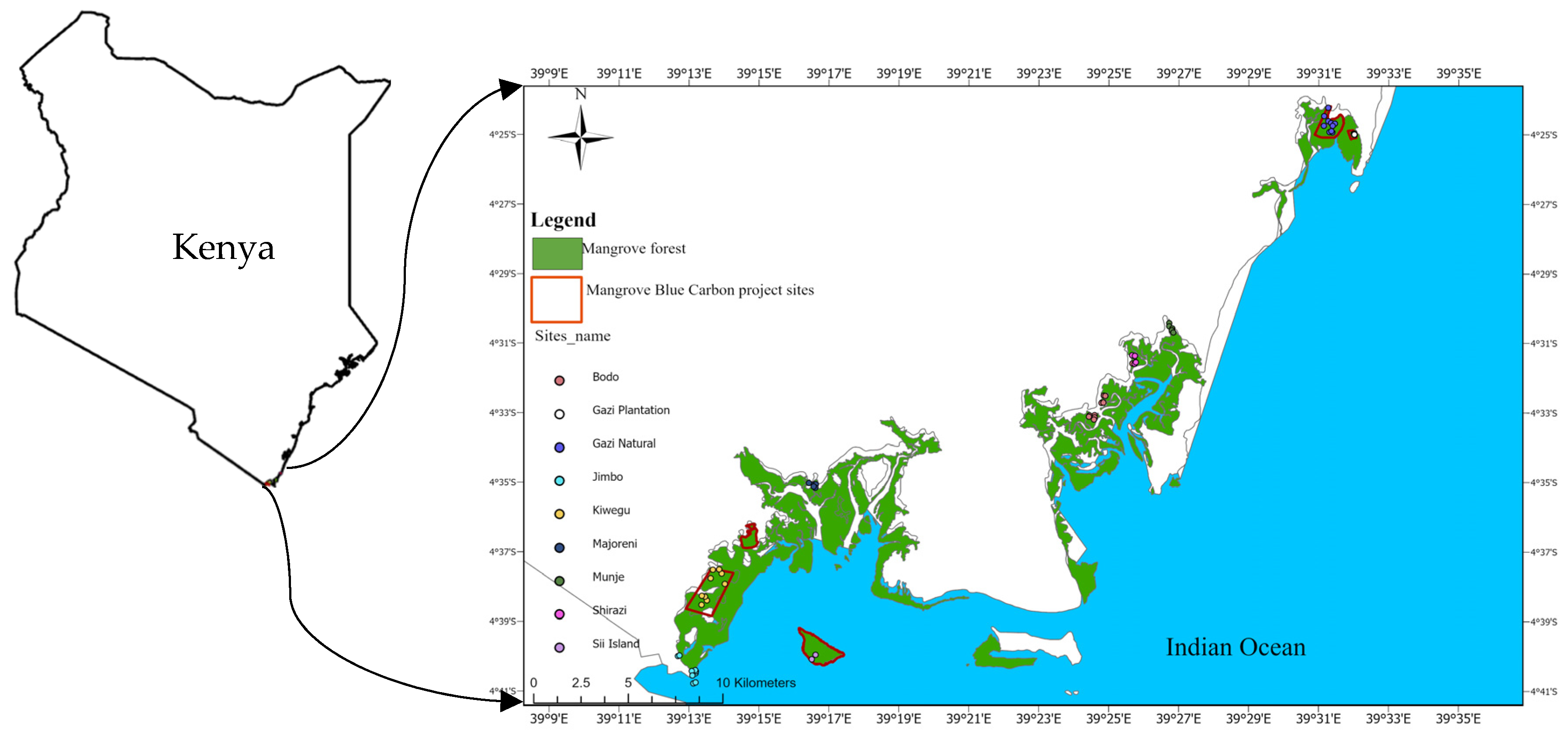
Figure 2.
Field-satellite carbon monitoring workflow. Field plot data (step 1-2) and satellite imagery (step 3b-5) are processed in parallel; only the 2025 model (step 5) is independently cross-validated. Step 6 compares the two independently derived estimates as a plausibility check, not a validation.
Figure 2.
Field-satellite carbon monitoring workflow. Field plot data (step 1-2) and satellite imagery (step 3b-5) are processed in parallel; only the 2025 model (step 5) is independently cross-validated. Step 6 compares the two independently derived estimates as a plausibility check, not a validation.
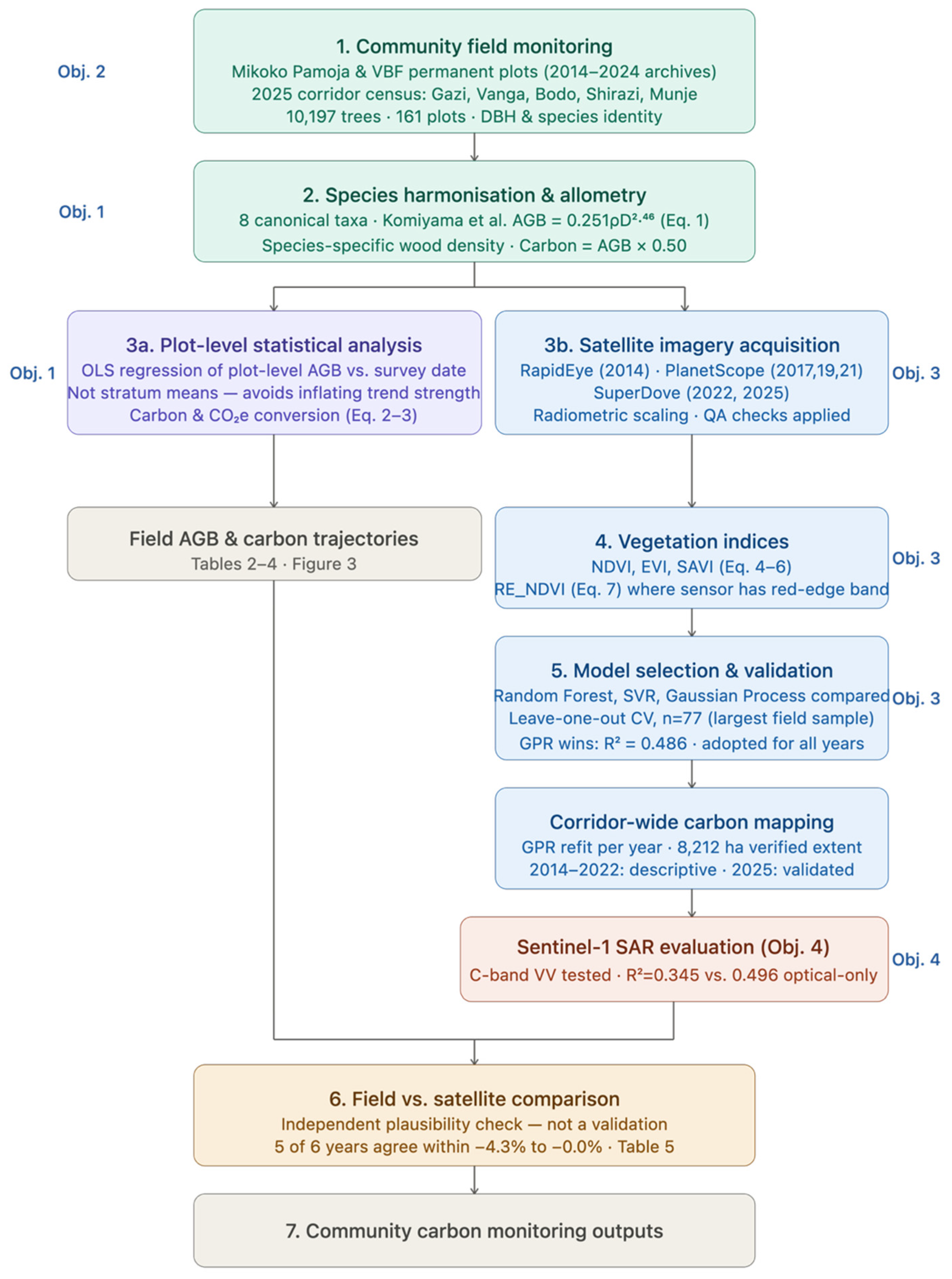
Figure 3.
Above-ground carbon stock trajectories and net gains, Gazi–Vanga mangrove corridor, Kenya, 2014–2025. (a) Stratum-mean carbon stock (Mg C ha−1) over time, derived from mean AGB values in Table 2 and Table 3 and a carbon fraction of 0.50.(b) Net carbon gain from each stratum’s baseline survey to its most recent survey.
Figure 3.
Above-ground carbon stock trajectories and net gains, Gazi–Vanga mangrove corridor, Kenya, 2014–2025. (a) Stratum-mean carbon stock (Mg C ha−1) over time, derived from mean AGB values in Table 2 and Table 3 and a carbon fraction of 0.50.(b) Net carbon gain from each stratum’s baseline survey to its most recent survey.
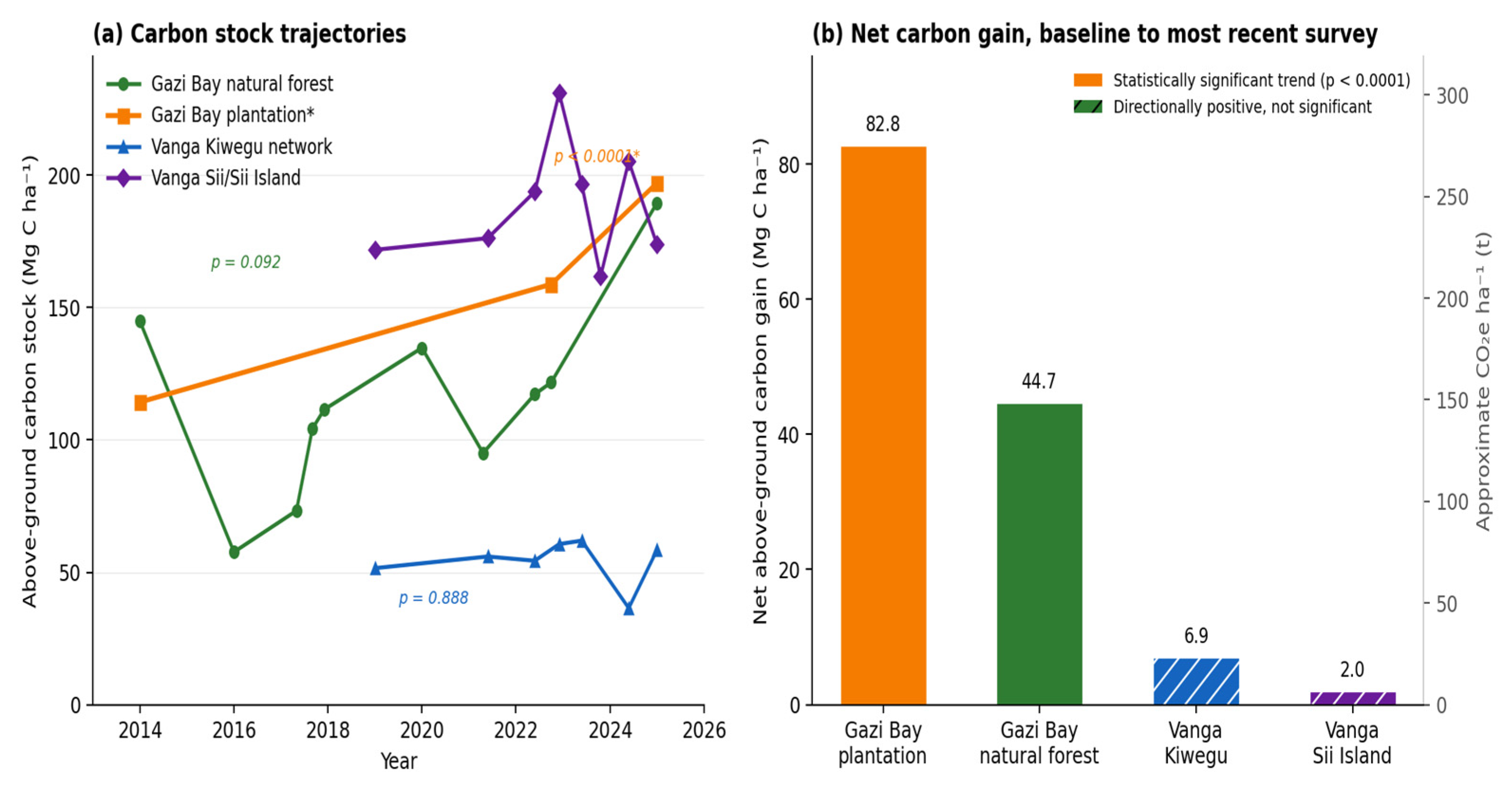
Figure 4.
Satellite-field carbon density comparison for the Gazi–Vanga corridor, Kenya, 2014–2025. Left panel: corridor-wide mean carbon density (Mg C ha−1) estimated from satellite imagery.
Figure 4.
Satellite-field carbon density comparison for the Gazi–Vanga corridor, Kenya, 2014–2025. Left panel: corridor-wide mean carbon density (Mg C ha−1) estimated from satellite imagery.
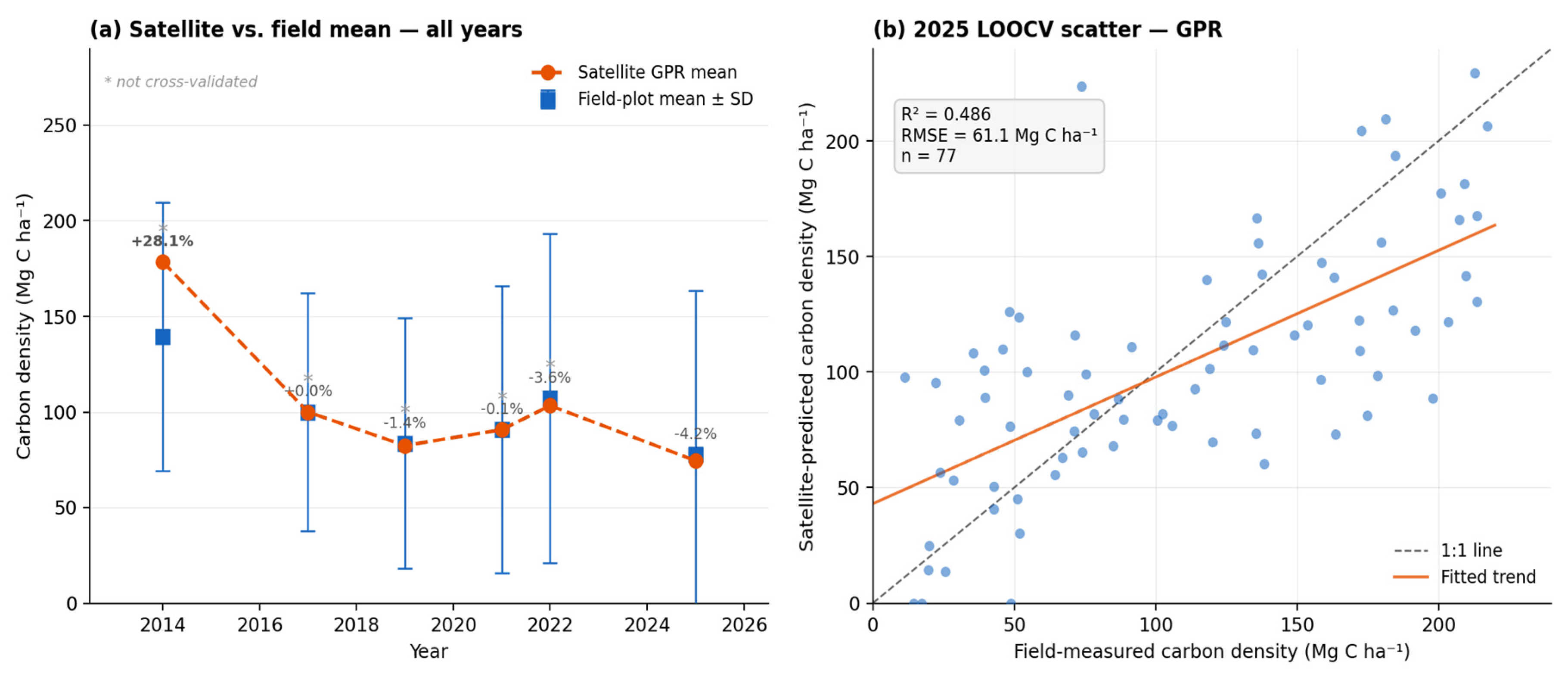
Figure 5.
Satellite-derived above-ground carbon density across the Gazi–Vanga corridor (8,212 ha), 2014, RapidEye, 5 m, n = 16 plots in Gazi Bay. Not validated.
Figure 5.
Satellite-derived above-ground carbon density across the Gazi–Vanga corridor (8,212 ha), 2014, RapidEye, 5 m, n = 16 plots in Gazi Bay. Not validated.
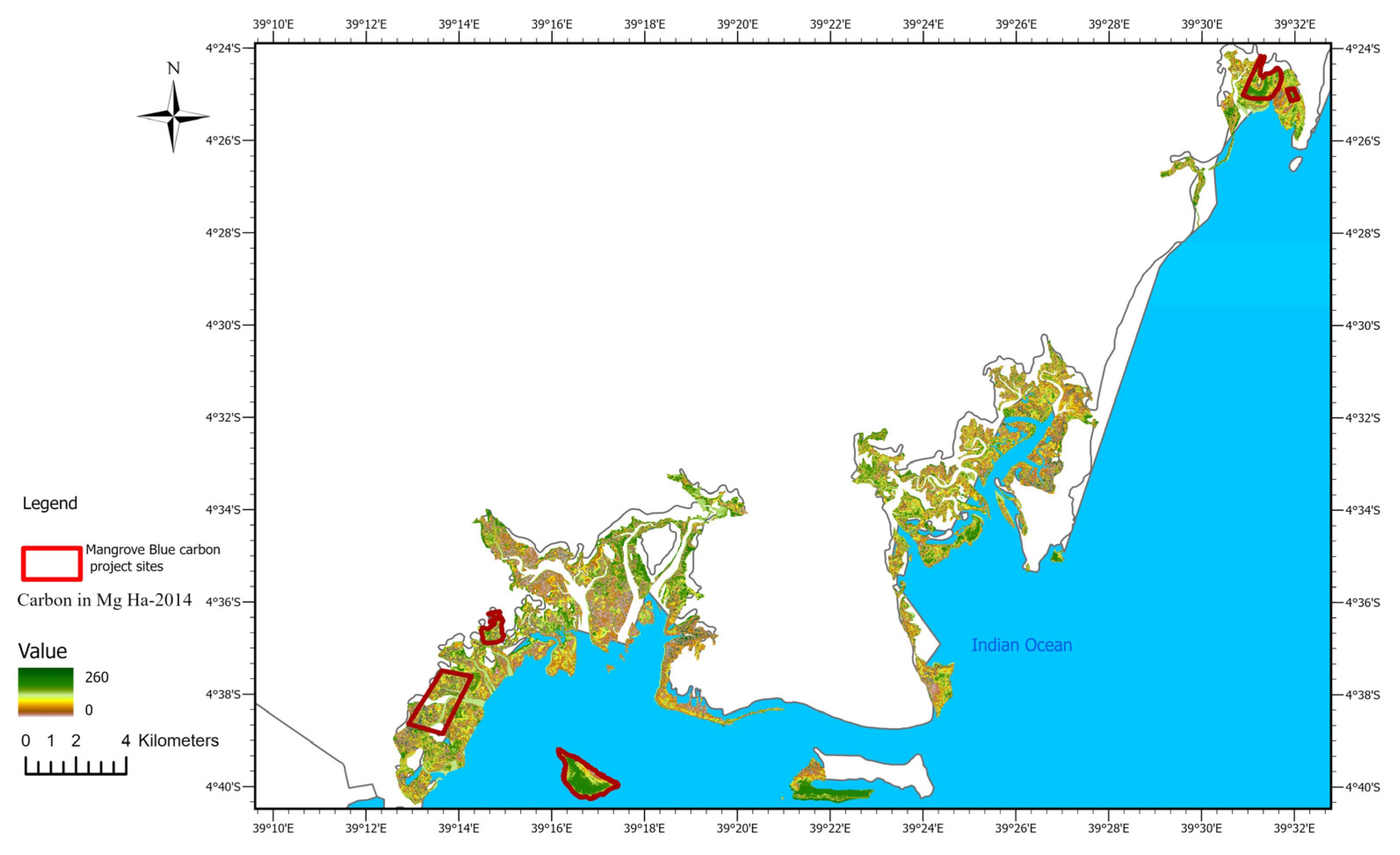
Figure 6.
Satellite-derived above-ground carbon density across the Gazi–Vanga corridor (8,212 ha), 2019, PlanetScope, 3–4 m, n = 15 plots. Not validated.
Figure 6.
Satellite-derived above-ground carbon density across the Gazi–Vanga corridor (8,212 ha), 2019, PlanetScope, 3–4 m, n = 15 plots. Not validated.
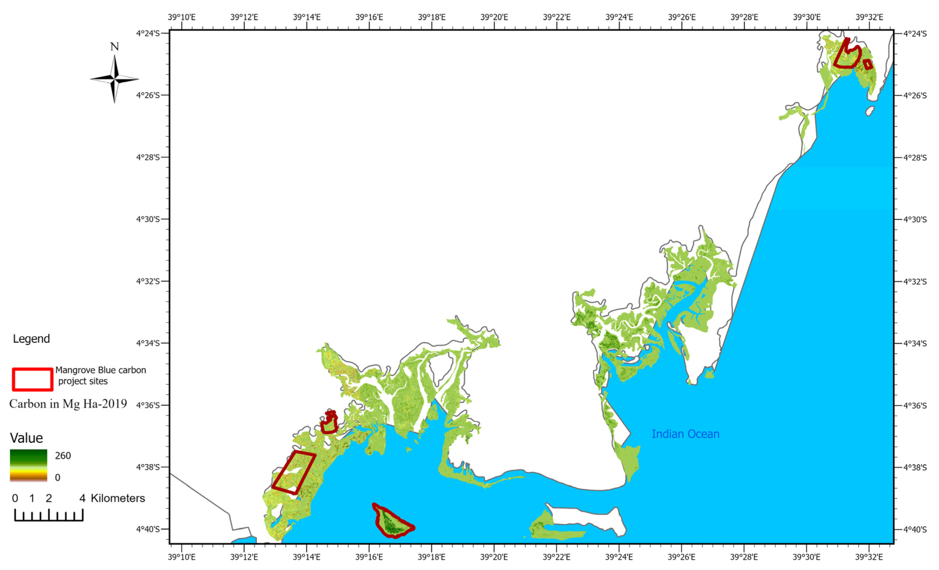
Figure 7.
Satellite-derived above-ground carbon density across the Gazi–Vanga corridor (8,212 ha), 2022, SuperDove, 3 m, n = 55 plots. Not validated.
Figure 7.
Satellite-derived above-ground carbon density across the Gazi–Vanga corridor (8,212 ha), 2022, SuperDove, 3 m, n = 55 plots. Not validated.
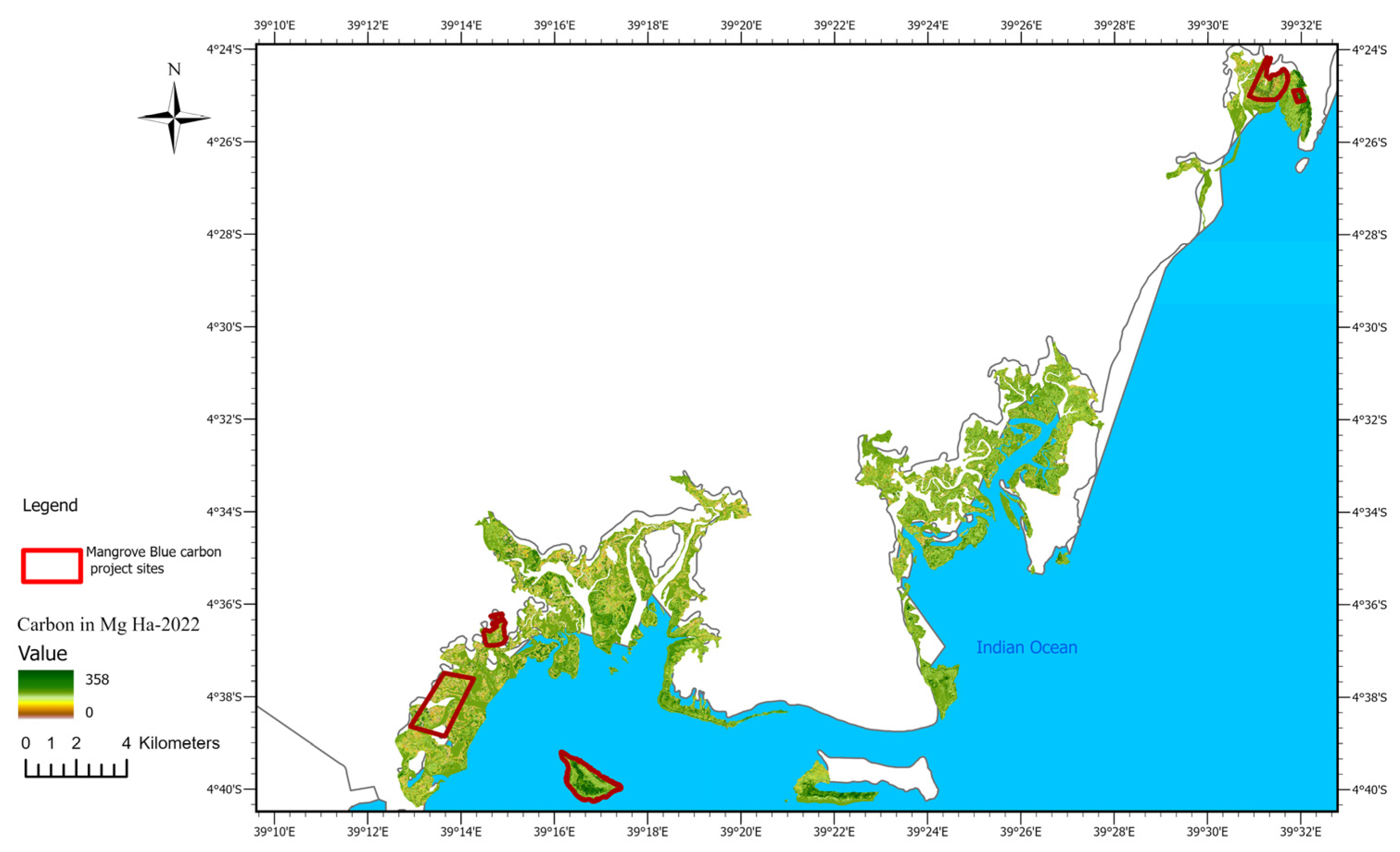
Figure 8.
Satellite-derived above-ground carbon density across the Gazi–Vanga corridor (8,212 ha), 2025, Super Dove, 3 m, n = 77 plots. Validated (R2 = 0.486).
Figure 8.
Satellite-derived above-ground carbon density across the Gazi–Vanga corridor (8,212 ha), 2025, Super Dove, 3 m, n = 77 plots. Validated (R2 = 0.486).
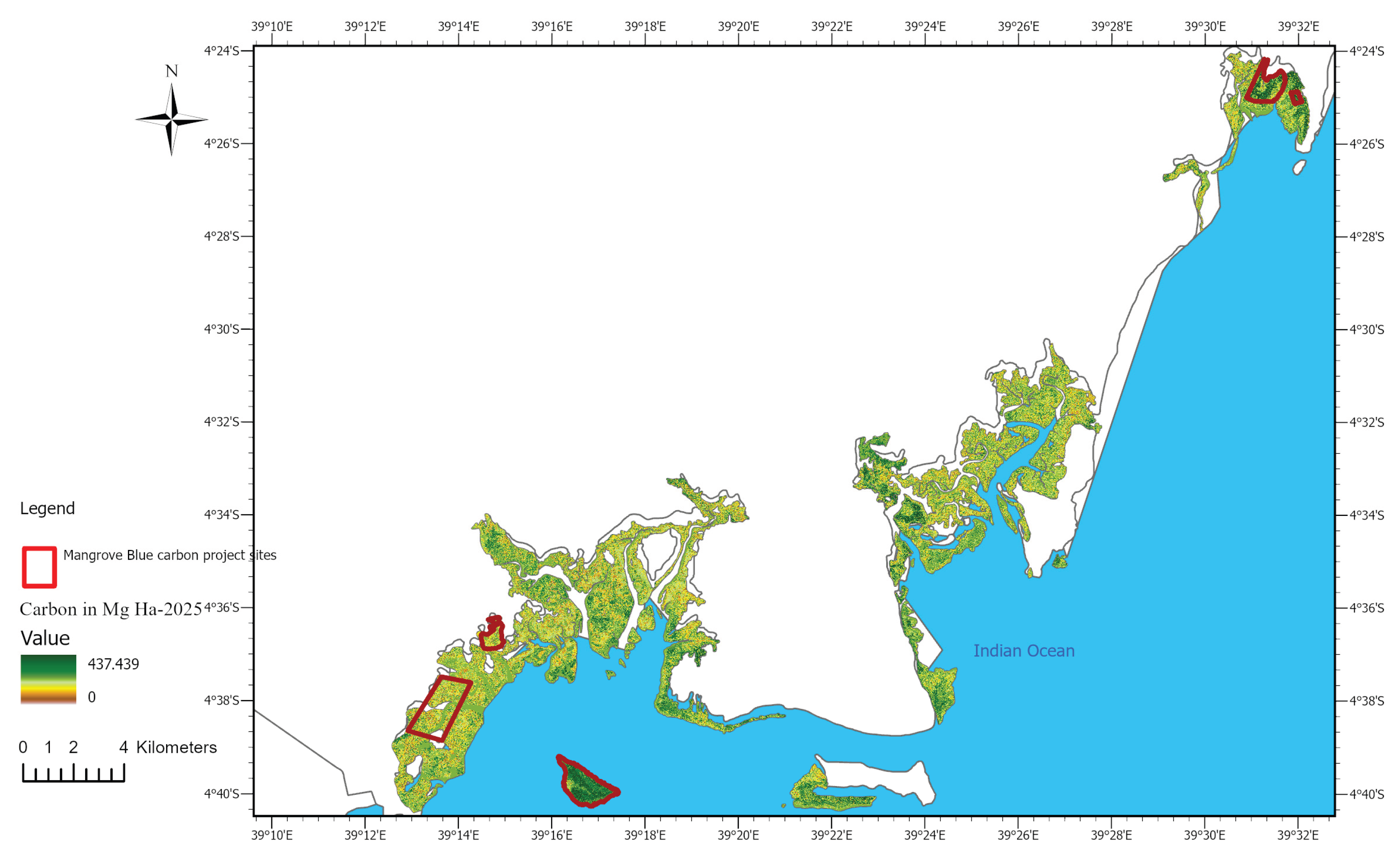
Table 1.
Plot network, survey years, and trajectory type across the study corridor. Kiwegu village plots, monitored under this grouping since 2019. Recorded separately in the 2025 field data directly under the VBF project’s own Kiwegu’ stratum labels.
Table 1.
Plot network, survey years, and trajectory type across the study corridor. Kiwegu village plots, monitored under this grouping since 2019. Recorded separately in the 2025 field data directly under the VBF project’s own Kiwegu’ stratum labels.
| Site | Stratum | n plots | Survey years | Trajectory type |
|---|---|---|---|---|
| Gazi Bay | Natural forest | 20/20/10/10/10 | 2014, 2017, 2020, 2022, 2025 | 5-epoch trajectory |
| Gazi Bay | Restoration plantation | 10/5/5 | 2017, 2022, 2025 | 3-epoch trajectory |
| Vanga | Kiwegu network | 11 (each yr) | 2019, 2021, 2023, 2024, 2025 | 5-epoch trajectory |
| Vanga | Sii Island | 4/4/4/4/6 | 2019, 2021, 2023, 2024, 2025 | 5-epoch trajectory |
| Vanga | Jimbo | 10 | 2025 | 2025 |
| Vanga | Majoreni | 6 | 2025 | 2025 |
| Vanga | Kiwegu (VBF stratum) | 9 | 2025 | 2025 |
| Vanga | Afforestation (Bazo/Makombe) | 4 | 2024 | Single epoch (new site) |
| Bodo | 7 village strata | 10 total | 2025 | 2025 |
| Shirazi | Kwaghafuru; KwaEdimundI | 4 total | 2025 | 2025 |
| Munje | Kwa makata; Mkawatsi | 6 total | 2025 | 2025 |
Table 2.
Allometric parameters and wood densities for eight mangrove species recorded in the Gazi–Vanga corridor, Kenya. AGB estimated using AGB = 0.251ρD2·46 (Komiyama et al., 2005); n = stems in harmonized dataset; ρ = wood density (g cm−3).
Table 2.
Allometric parameters and wood densities for eight mangrove species recorded in the Gazi–Vanga corridor, Kenya. AGB estimated using AGB = 0.251ρD2·46 (Komiyama et al., 2005); n = stems in harmonized dataset; ρ = wood density (g cm−3).
| Species | ρ (g cm−3) | AGB equation (kg) | n stems | % | ρ source |
|---|---|---|---|---|---|
| Rhizophora mucronata | 0.701 | 0.251 × 0.701 × DBH2·46 | ~5,800 | ~57 | (a) |
| Ceriops tagal | 0.746 | 0.251 × 0.746 × DBH2·46 | ~2,400 | ~24 | (a) |
| Bruguiera gymnorrhiza | 0.699 | 0.251 × 0.699 × DBH2·46 | ~800 | ~8 | (a) |
| Sonneratia alba | 0.475 | 0.251 × 0.475 × DBH2·46 | ~350 | ~3 | (a) |
| Avicennia marina | 0.650 | 0.251 × 0.650 × DBH2·46 | ~500 | ~5 | (b) proxy |
| Xylocarpus granatum | 0.528 | 0.251 × 0.528 × DBH2·46 | ~270 | ~3 | (a) |
| Xylocarpus moluccensis | 0.531 | 0.251 × 0.531 × DBH2·46 | ~70 | <1 | (a) |
| Lumnitzera racemosa | 0.700 | 0.251 × 0.700 × DBH2·46 | ~7 | <0.1 | (c) flagged proxy |
Table 3.
Spectral vegetation indices used as predictors in the Gaussian Process Regression model.
| Index | Formula | Sensors | Rationale for inclusion |
|---|---|---|---|
| NDVI | NDVI = (NIR − Red) / (NIR + Red) (Eq. 4) | All (2014–2025) | Standard chlorophyll-related canopy greenness; widely applied in mangrove biomass mapping [35,36]. |
| EVI | EVI = 2.5 × (NIR − Red) / (NIR + 6×Red − 7.5×Blue + 1) (Eq. 5) | All (2014–2025) | Atmospheric and soil-background noise correction; improved sensitivity in high-biomass closed canopy; best-performing index in [35] for mangrove AGC. |
| SAVI | SAVI = 1.5 × (NIR − Red) / (NIR + Red + 0.5) (Eq. 6) | All (2014–2025) | Soil background correction at canopy edges and in degraded stands; relevant for heterogeneous Bodo and Munje strata. |
| RE_NDVI | RE_NDVI = (NIR − RedEdge) / (NIR + RedEdge) (Eq. 7) | RapidEye (2014); SuperDove (2022, 2025) only | Red-edge sensitive to canopy structure and chlorophyll at wavelengths where standard red-band indices saturate in dense closed-canopy mangrove [35,36]. |
1 Computed from annual surface-reflectance composites. 2 RE_NDVI available for RapidEye and SuperDove only; not available for 4-band PlanetScope (2017, 2019, 2021). 3 EVI coefficients: G = 2.5, C1 = 6, C2 = 7.5, L = 1. NIR = near-infrared; RE = red-edge; ρ = surface reflectance in subscripted band; Mg C ha−1 = megagrams of carbon per hectare.
Table 5.
restoration plantation stratum, plots randomly relocated at each survey round (PMP1–PMP10).
Table 5.
restoration plantation stratum, plots randomly relocated at each survey round (PMP1–PMP10).
| Year | n | Mean (Mg/ha) | Median (Mg/ha) |
|---|---|---|---|
| 2014 | 6 | 228.6 | 212.5 |
| 2017-11 | 10 | 199.3 | 206.1 |
| 2022-09 | 5 | 317.7 | 305.8 |
| 2025 | 5 | 394.2 | 391.9 |
Table 6.
AGB at Vanga Blue Forest, Kwale County, Kenya, by survey year: (a) Kiwegu village network (permanent plots VPMP1–VPMP15 across six villages).
Table 6.
AGB at Vanga Blue Forest, Kwale County, Kenya, by survey year: (a) Kiwegu village network (permanent plots VPMP1–VPMP15 across six villages).
| Year | n | Mean (Mg/ha) | Median (Mg/ha) |
| 2019 | 11 | 103.1 | 105.2 |
| 2021-05 | 11 | 111.9 | 98.3 |
| 2022-05 | 11 | 108.7 | 118.1 |
| 2022-11 | 11 | 121.3 | 119.6 |
| 2023-05 | 11 | 123.9 | 120.2 |
| 2024-05 | 11 | 72.9 | 67.0 |
| 2025 | 11 | 116.8 | 126.2 |
Table 7.
AGB at Vanga Blue Forest, Kwale County, Kenya, by survey year: Sii Island stratum (permanent plots).
Table 7.
AGB at Vanga Blue Forest, Kwale County, Kenya, by survey year: Sii Island stratum (permanent plots).
| Year | n | Mean (Mg/ha) | Median (Mg/ha) |
| 2019 | 4 | 343.7 | 342.9 |
| 2021-05 | 4 | 352.5 | 350.2 |
| 2022-05 | 4 | 387.7 | 364.3 |
| 2022-11 | 4 | 462.2 | 378.2 |
| 2023-05 | 4 | 393.3 | 371.5 |
| 2023-10 | 5 | 323.6 | 230.0 |
| 2024-05 | 4 | 410.7 | 385.3 |
| 2025 | 6 | 347.7 | 312.8 |
Table 8.
(AGB) at sites surveyed for the first time in 2025, Gazi–Vanga corridor, Kenya.
| Area | Stratum | n | AGB (Mg/ha) | SE |
| Bodo | Ali Asa | 2 | 60.4 | 0.8 |
| Bodo | Chupaani | 1 | 102.8 | n/a |
| Bodo | Kimeku | 2 | 85.7 | 1.6 |
| Bodo | Kwa Kea | 1 | 98.6 | n/a |
| Bodo | Kwa Mbwea | 2 | 66.3 | 27.0 |
| Bodo | Kwa Mphiya | 1 | 99.2 | n/a |
| Bodo | Uwanja wa Shule | 1 | 13.7 | n/a |
| Bodo (area mean) | all strata pooled | 10 | 73.9 | 9.4 |
| Shirazi | KwaEdimundI | 2 | 79.7 | 7.9 |
| Shirazi | Kwaghafuru | 2 | 104.3 | 24.9 |
| Munje | Kwa makata | 4 | 59.9 | 18.8 |
| Munje | Mkawatsi | 2 | 100.2 | 32.0 |
| Vanga | Jimbo | 10 | 57.9 | 11.3 |
| Vanga | Majoreni | 6 | 39.8 | 13.3 |
| Vanga | Kiwegu (VBF stratum) ‡ | 9 | 78.8 | 20.2 |
| Vanga (area mean) | Jimbo+Majoreni+Kiwegu‡+ SiiI sl. | 31 | 116.5 | 23.8 |
Table 9.
Leave-one-out cross-validation comparison of three machine learning algorithms, 2025 (n = 77).
Table 9.
Leave-one-out cross-validation comparison of three machine learning algorithms, 2025 (n = 77).
| Model | n | R2 | RMSE (Mg C ha−1) | MAE (Mg C ha−1) |
| Random Forest | 77 | 0.324 | 70.0 | 43.4 |
| Support Vector Regression | 77 | 0.229 | 74.8 | 43.0 |
| Gaussian Process Regression | 77 | 0.486 | 61.1 | 39.0 |
Table 10.
Satellite-derived and field-extrapolated above-ground carbon density across the 8,212 ha Gazi–Vanga corridor by year, sensor, and validation status (Gaussian Process Regression; 2025 formally validated: R2 = 0.486, RMSE = 61.1 Mg C ha−1; all other years are descriptive estimates).
Table 10.
Satellite-derived and field-extrapolated above-ground carbon density across the 8,212 ha Gazi–Vanga corridor by year, sensor, and validation status (Gaussian Process Regression; 2025 formally validated: R2 = 0.486, RMSE = 61.1 Mg C ha−1; all other years are descriptive estimates).
| Year | n | Validation | Satellite mean (Mg C/ha) | Field mean (Mg C/ha) | Diff. | Satellite total (Mg C) | Field-extrap total (Mg C) |
|---|---|---|---|---|---|---|---|
| 2014 | 16 | Not validated | 178.6 | 139.4 ± 70.2 | +28.1% | 1,466,389 | 1,144,419 |
| 2017 | 50 | Not validated | 100.0 | 100.0 ± 62.4 | −0.0% | 821,424 | 821,485 |
| 2019 | 15 | Not validated | 82.4 | 83.6 ± 65.6 | −1.4% | 676,869 | 686,768 |
| 2021 | 25 | Not validated | 90.7 | 90.8 ± 75.0 | −0.1% | 745,058 | 746,022 |
| 2022 | 55 | Not validated | 103.3 | 107.2 ± 86.2 | −3.7% | 847,931 | 880,208 |
| 2025 | 77 | Validated, R2=0.486 | 74.5 | 77.8 ± 85.8 | −4.3% | 611,659 | 639,178 |
Disclaimer/Publisher’s Note: The statements, opinions and data contained in all publications are solely those of the individual author(s) and contributor(s) and not of MDPI and/or the editor(s). MDPI and/or the editor(s) disclaim responsibility for any injury to people or property resulting from any ideas, methods, instructions or products referred to in the content. |
© 2026 by the authors. Licensee MDPI, Basel, Switzerland. This article is an open access article distributed under the terms and conditions of the Creative Commons Attribution (CC BY) license (http://creativecommons.org/licenses/by/4.0/).
Copyright: This open access article is published under a Creative Commons CC BY 4.0 license, which permit the free download, distribution, and reuse, provided that the author and preprint are cited in any reuse.


