A Reproducible COMSOL Multiphysics Workflow for Coupled Vibroacoustic Simulation of Electric-Vehicle Gearboxes under Manufacturing, Assembly, and Operating Variability

1. Introduction

The tonal character of electric-vehicle drivetrains has shifted gearbox noise from a secondary masking problem to a primary design constraint. The absence of dominant combustion noise exposes gear-mesh orders, sidebands, bearing-related modulation, and structural resonances over a broad operating range. Reliable prediction therefore requires more than a stand-alone tooth-contact or housing finite element calculation. The excitation, transmission path, and radiating structure must be represented in a connected numerical chain.

A conventional workflow is often distributed among several specialized tools. Gear macro- and microgeometry are evaluated by tooth-contact analysis; dynamic forces are computed in a torsional or multibody model; housing vibration is obtained in a structural finite element model; and the resulting surface motion is transferred to an acoustic solver. This separation is technically effective, but it creates recurring problems in research practice: parameter definitions are duplicated, coordinate systems are not always traceable, interpolation between meshes can obscure energy transfer, and uncertainty introduced by manufacturing and assembly is difficult to propagate consistently.

COMSOL Multiphysics offers a different integration strategy. Its documented gear-pair features include gear elasticity, transmission error, backlash, and friction; rotor formulations can be connected to bearings and flexible foundations; structural interfaces support static, modal, transient, and frequency-response studies; and the Acoustics Module provides both finite-element and boundary-element formulations for radiated sound [1,2,3,4]. The same model can also contain parametric sweeps and application-level methods. This makes COMSOL attractive as an integration environment even when detailed tooth-contact quantities originate in an external LTCA or measurement workflow.

The objective of this paper is not to claim that a general-purpose multiphysics package replaces every specialized gearbox tool. Instead, it defines a transparent division of tasks: tooth-contact solvers or measurement processing generate the local excitation descriptors, while COMSOL propagates those descriptors through the rotor-bearing-housing system and into the acoustic field. The paper contributes (i) a hierarchical model-fidelity strategy, (ii) a step-by-step COMSOL implementation sequence, (iii) a variability-aware parameter architecture, (iv) a verification and experimental-validation protocol, and (v) a fully specified reduced-order benchmark that can be reproduced independently and used to check the COMSOL model before proprietary geometry is introduced.

The proposed framework is intended for electric-vehicle parallel-axis or planetary gearboxes, but the same structure is applicable to other geared power-transmission systems. The implementation is based on COMSOL Multiphysics 6.4 and the corresponding module documentation [1,2,3,4,5,6].

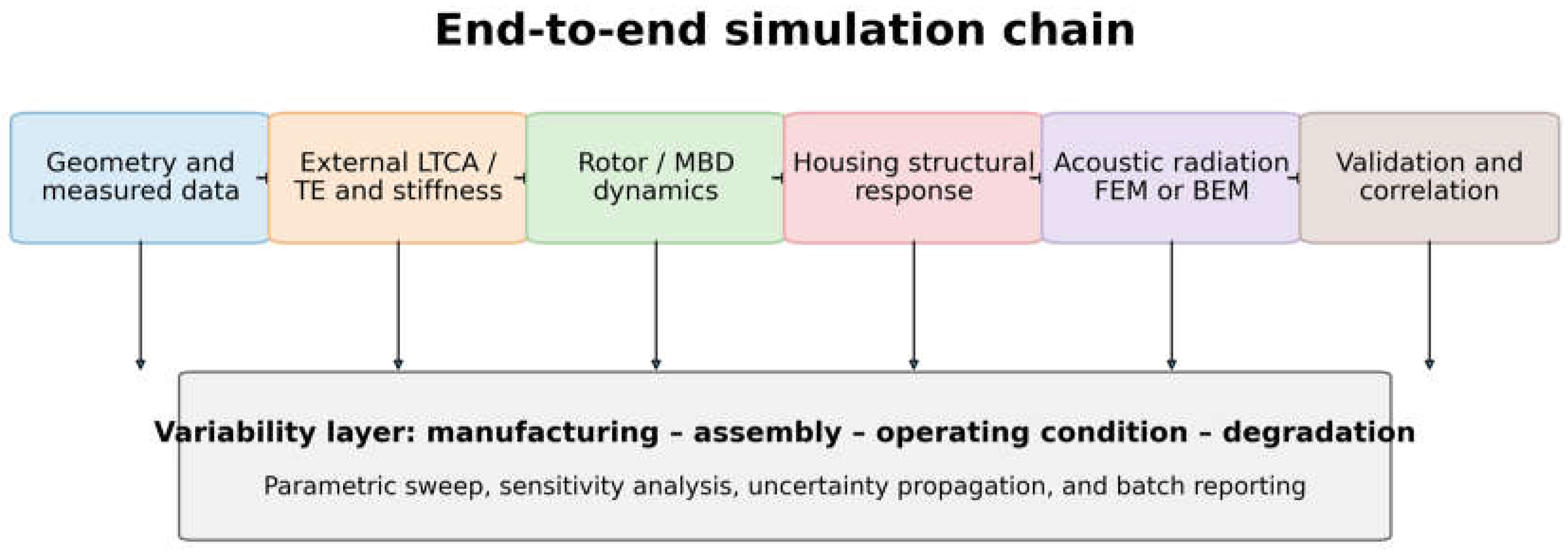
Figure 1. End-to-end variability-aware simulation chain proposed for COMSOL-based gearbox vibroacoustics.

Figure 1. End-to-end variability-aware simulation chain proposed for COMSOL-based gearbox vibroacoustics.

2. Scope, Model Boundaries, and Main Contributions

The workflow covers structure-borne excitation generated by gear meshing and transmitted through shafts, bearings, joints, and the housing to the surrounding acoustic medium. It is designed around a baseline/recommended/advanced hierarchy rather than a single mandatory model. This is important because the appropriate level of detail depends on the research question. A housing-design screening study does not require the same tooth-level detail as a study of backlash-induced rattle or tooth-to-tooth manufacturing variability.

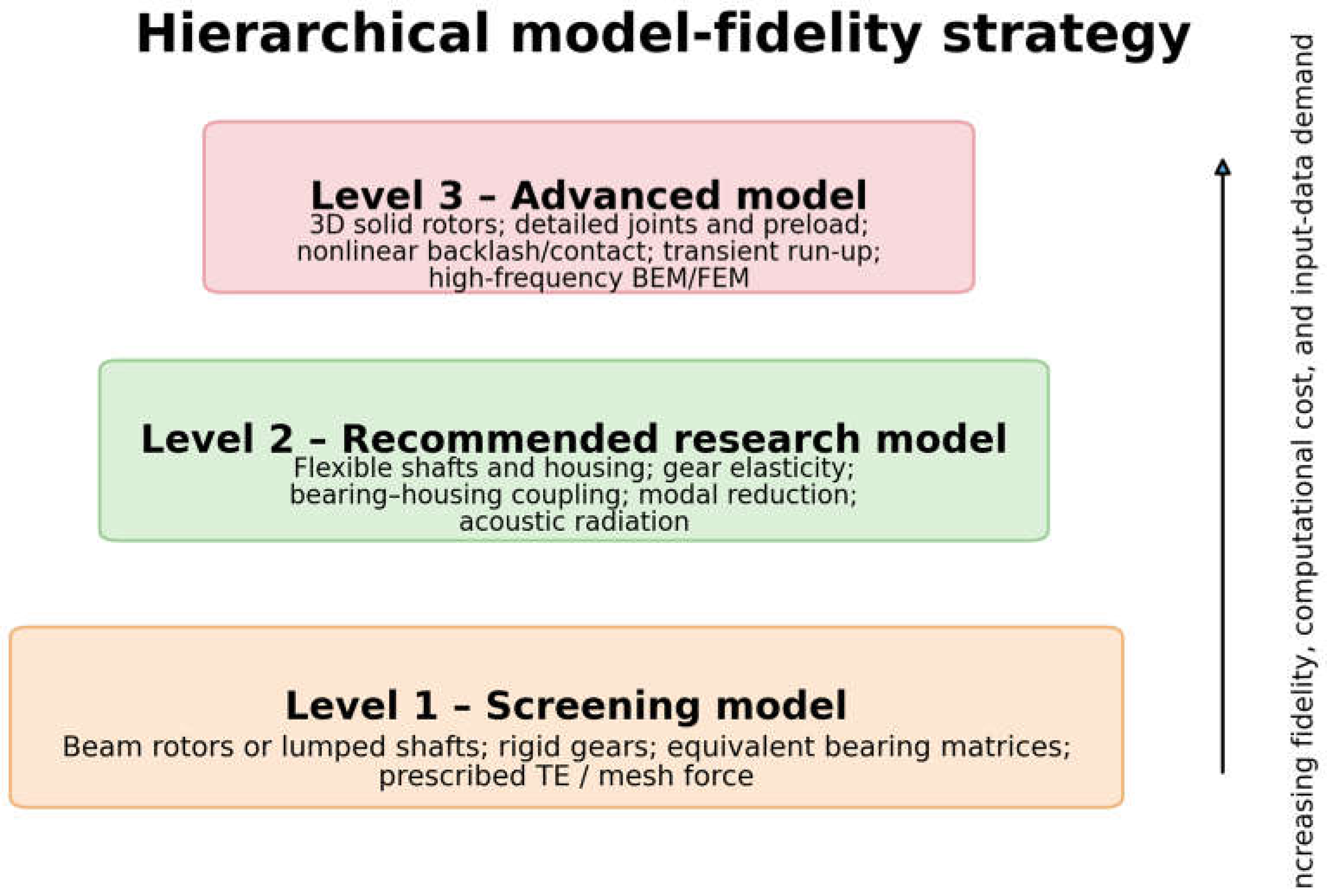
The baseline model uses prescribed harmonic forces or TE functions and equivalent support properties. The recommended model adds periodic mesh stiffness, flexible shafts and housing, bearing-foundation coupling, and a frequency-domain radiation model. The advanced model adds nonlinear backlash, transient contact events, speed ramps, three-dimensional solid rotor formulations, and high-frequency acoustic treatment. Each higher level should only be accepted when it changes a target output by more than the predefined engineering tolerance.

The reviewed COMSOL guides document parameterized gear geometries and gear-pair properties, but they do not document direct import of measured CMM flank maps or a native tooth-indexed topography field into the gear-pair contact formulation. Consequently, measured surface data should be reduced externally to functions that the system model can use: quasi-static TE, mesh stiffness, mesh damping, contact ratio, runout, phase, or equivalent force histories. A custom contact formulation is possible in principle, but it is outside the baseline workflow and must be verified separately.

Table 1. Main methodological contributions of the proposed workflow.

Contribution	Purpose	Primary output
Unified model architecture	Connects excitation, rotor-bearing dynamics, housing vibration, and acoustics in one parameter structure.	Traceable data flow and consistent coordinate systems
Fidelity hierarchy	Prevents unnecessary model complexity and supports staged verification.	Level 1, Level 2, and Level 3 model definitions
External LTCA/measurement bridge	Introduces microgeometry and measured variability without claiming undocumented direct topography contact.	TE, k_m, c_m, runout, and force functions
Verification and validation protocol	Separates numerical convergence, subsystem checks, and experimental correlation.	Mesh error, MAC, FRF error, SPL error
Automation and reporting structure	Enables reproducible parametric studies and consistent export.	Parameter manifests, result tables, and batch reports

Table 1. Main methodological contributions of the proposed workflow.

Contribution	Purpose	Primary output
Unified model architecture	Connects excitation, rotor-bearing dynamics, housing vibration, and acoustics in one parameter structure.	Traceable data flow and consistent coordinate systems
Fidelity hierarchy	Prevents unnecessary model complexity and supports staged verification.	Level 1, Level 2, and Level 3 model definitions
External LTCA/measurement bridge	Introduces microgeometry and measured variability without claiming undocumented direct topography contact.	TE, k_m, c_m, runout, and force functions
Verification and validation protocol	Separates numerical convergence, subsystem checks, and experimental correlation.	Mesh error, MAC, FRF error, SPL error
Automation and reporting structure	Enables reproducible parametric studies and consistent export.	Parameter manifests, result tables, and batch reports

Figure 2. Hierarchical model-fidelity strategy for screening, recommended research, and advanced nonlinear analyses.

Figure 2. Hierarchical model-fidelity strategy for screening, recommended research, and advanced nonlinear analyses.

3. Theoretical Framework

3.1. Gear-Mesh Excitation

For a gear pair with pinion tooth count z_p and rotational speed n_p in revolutions per minute, the fundamental gear-mesh frequency is

f_m = z_p n_p / 60 = z_g n_g / 60 (1)

Harmonics of f_m and modulation by shaft-order, runout, eccentricity, and load variation form the primary deterministic excitation set. In a frequency-domain model, each order can be solved directly. In a transient model, the same information is represented as an angle- or time-dependent function.

A practical representation of static transmission error is a Fourier or tabulated periodic function:

e(phi) = e_0 + sum[h=1..H] E_h cos(h phi + psi_h) (2)

where phi is the mesh-cycle angle. The mesh stiffness can be represented similarly:

k_m(phi) = k_bar [1 + sum[h=1..H] kappa_h cos(h phi + chi_h)] (3)

The equivalent mesh force acting along the line of action is then written in a compact form as

F_m = k_m(phi) g(delta - e) + c_m d[g(delta - e)]/dt (4)

where delta is the relative displacement projected onto the line of action and g(.) is the backlash function. For a linear whine analysis, g(x)=x and the equations may be linearized around the loaded operating point. For rattle or loss of contact, g(.) must retain the dead-zone nonlinearity and the solution is time dependent. COMSOL gear-pair nodes provide documented inputs for mesh stiffness, mesh damping, contact ratio, static TE, backlash, and friction [2,3].

3.2. Rotor-Bearing-Housing Dynamics

The assembled structural system can be expressed as

M q_ddot + C q_dot + K q = B_m F_m + F_ext (5)

where M, C, and K are the global mass, damping, and stiffness matrices and B_m maps the mesh force to the selected gear degrees of freedom. The matrices include shaft bending and torsion, housing flexibility, joint and foundation properties, and bearing coupling. In a harmonic analysis at angular frequency omega, the complex response follows

[-omega^2 M + i omega C + K] q_hat = F_hat (6)

The rotor model can be constructed with Beam Rotor, Solid Rotor, Solid Rotor in a fixed frame, or Multibody Dynamics. Beam formulations are efficient for early system studies. Solid-rotor formulations are appropriate when shaft geometry, local flexibility, or rotating-frame effects are central. COMSOL requires the rotation axis and base point to be defined for solid-rotor models. In the rotating frame, centrifugal, Coriolis, and Euler contributions are introduced through the Rotating Frame feature [2].

Rolling bearings may be represented by equivalent matrices, detailed built-in roller-bearing formulations, or calibrated foundation properties. The documented radial roller-bearing models include common ball and roller bearing families, clearance, preload, race and roller material properties, and fixed, moving, flexible, or squeeze-film-damper foundations [2,3]. Connecting a bearing foundation to an Attachment or a rigid/flexible housing domain provides a direct rotor-to-stator coupling path.

3.3. Structural-Acoustic Coupling

The linear pressure-acoustics field in a homogeneous fluid is governed in the frequency domain by the Helmholtz equation. In one common form,

nabla . (1/rho_f nabla p) + omega^2 p/(rho_f c_f^2) = 0 (7)

At the fluid-solid boundary, acoustic pressure produces a normal traction on the structure and structural normal acceleration excites the fluid. COMSOL's Acoustic-Solid Interaction, Frequency Domain interface adds Pressure Acoustics, Solid Mechanics, and the Acoustic-Structure Boundary coupling in one predefined configuration [4]. The coupled boundary relations can be summarized as

t_s = -p n, partial(p)/partial(n) = rho_f omega^2 u_n (8)

with the sign depending on the adopted harmonic convention. The sound pressure level at a receiver is

L_p = 20 log10(|p_rms| / p_ref), p_ref = 20 microPa (9)

For exterior radiation, a finite air domain terminated by a PML or radiation condition can be used. Alternatively, the Pressure Acoustics, Boundary Elements interface represents the infinite exterior domain using only boundary meshes. The latter is attractive for gearbox radiation because the surrounding air volume does not need to be volume meshed, although BEM matrices are dense and solver memory must be considered [4].

4. COMSOL Model Architecture

4.1. Required Modules and Their Roles

Table 2. Mapping of research tasks to COMSOL modules and interfaces.

Task	COMSOL interface or module	Implementation note
CAD preparation	CAD Import Module	Import STEP, Parasolid, ACIS, or native formats; repair, defeature, and retain NVH-relevant ribs, covers, bearing seats, and mounting regions.
Gear and drivetrain kinematics	Multibody Dynamics Module	Rigid/flexible parts, gear pairs, joints, attachments, gear elasticity, TE, backlash, and friction.
Rotating shafts and bearings	Rotordynamics Module	Beam Rotor or Solid Rotor; bearing types, preload, clearance, flexible foundations, misalignment, and speed-dependent studies.
Housing vibration	Structural Mechanics Module	Solid, shell, or mixed model; prestress, eigenfrequency, frequency response, transient response, and CMS.
Airborne radiation	Acoustics Module	Acoustic-Solid Interaction, Pressure Acoustics FEM, exterior-field evaluation, or Pressure Acoustics BEM.
Automation and deployment	Application Builder / model methods	Parameter checks, batch execution, predefined plots, tables, and report export.

Table 2. Mapping of research tasks to COMSOL modules and interfaces.

Task	COMSOL interface or module	Implementation note
CAD preparation	CAD Import Module	Import STEP, Parasolid, ACIS, or native formats; repair, defeature, and retain NVH-relevant ribs, covers, bearing seats, and mounting regions.
Gear and drivetrain kinematics	Multibody Dynamics Module	Rigid/flexible parts, gear pairs, joints, attachments, gear elasticity, TE, backlash, and friction.
Rotating shafts and bearings	Rotordynamics Module	Beam Rotor or Solid Rotor; bearing types, preload, clearance, flexible foundations, misalignment, and speed-dependent studies.
Housing vibration	Structural Mechanics Module	Solid, shell, or mixed model; prestress, eigenfrequency, frequency response, transient response, and CMS.
Airborne radiation	Acoustics Module	Acoustic-Solid Interaction, Pressure Acoustics FEM, exterior-field evaluation, or Pressure Acoustics BEM.
Automation and deployment	Application Builder / model methods	Parameter checks, batch execution, predefined plots, tables, and report export.

4.2. Data Hierarchy and Parameter Naming

The model should be parameter driven from the beginning. Geometry dimensions, operating conditions, material data, bearing properties, excitation descriptors, and solver controls should not be entered as isolated numbers in physics nodes. They should be declared in Global Definitions or imported from version-controlled parameter files. A consistent prefix convention reduces ambiguity: geo_ for geometry, mat_ for materials, op_ for operating conditions, gr_ for gear data, brg_ for bearings, hsg_ for housing, ac_ for acoustics, and sol_ for solver controls.

Table 3. Minimum input-data structure for a traceable model.

Parameter group	Examples	Preferred source
Gear macrogeometry	z, module, pressure angle, helix angle, face width, center distance	Design model or verified gear calculation
Mesh excitation	e(phi), k_m(phi), c_m, contact ratio, phase, runout	LTCA, measurement processing, or calibrated analytical model
Operating condition	Input speed, torque, temperature, direction of rotation	Test plan or duty cycle
Bearings	Type, clearance, preload, geometry, stiffness/damping, misalignment	Supplier data, detailed bearing model, or identification
Housing and joints	Material, wall thickness, bolt preload, mount stiffness, damping	CAD/BOM, material test, EMA calibration
Acoustic domain	Fluid density, sound speed, receiver coordinates, frequency range	Test environment and ambient conditions
Variability	Distribution, tolerance, correlation, sample identifier	CMM, process capability, assembly data, or engineering assumption

Table 3. Minimum input-data structure for a traceable model.

Parameter group	Examples	Preferred source
Gear macrogeometry	z, module, pressure angle, helix angle, face width, center distance	Design model or verified gear calculation
Mesh excitation	e(phi), k_m(phi), c_m, contact ratio, phase, runout	LTCA, measurement processing, or calibrated analytical model
Operating condition	Input speed, torque, temperature, direction of rotation	Test plan or duty cycle
Bearings	Type, clearance, preload, geometry, stiffness/damping, misalignment	Supplier data, detailed bearing model, or identification
Housing and joints	Material, wall thickness, bolt preload, mount stiffness, damping	CAD/BOM, material test, EMA calibration
Acoustic domain	Fluid density, sound speed, receiver coordinates, frequency range	Test environment and ambient conditions
Variability	Distribution, tolerance, correlation, sample identifier	CMM, process capability, assembly data, or engineering assumption

4.3. Geometry Representation

The housing should retain features that influence modal density, local stiffness, or radiation efficiency. Bearing seats, cover interfaces, ribs, mounting lugs, large fillets, and plate-like panels are normally retained. Small cosmetic holes, logos, tiny chamfers, and manufacturing details that do not influence stiffness or mass may be removed. Geometry simplification must be documented by mass-property and modal comparisons.

Three representation options are recommended. A full-solid housing is robust at low and medium frequencies but can become expensive. A midsurface shell model is efficient for thin cast or sheet-like regions but requires careful treatment of intersections, joints, and local bearing seats. A mixed solid-shell model often offers the best compromise: bearing seats and thick bosses remain solid, while broad covers and walls are represented by shells. The CAD Import Module provides tools for import, repair, defeaturing, interference detection, and face replacement [5].

4.4. Model-Fidelity Levels

Table 4. Recommended hierarchy of model fidelity.

Feature	Level 1: baseline	Level 2: recommended	Level 3: advanced
Gear excitation	Harmonic mesh force or TE order set	Periodic TE and mesh stiffness from LTCA	Tooth-indexed or transient excitation; nonlinear contact representation
Shafts	Beam or lumped torsional elements	Beam or flexible 3D shafts	Solid rotor with local geometry and rotating-frame effects
Bearings	Equivalent linear matrices	Built-in bearing or identified nonlinear tangent properties	Clearance, preload, misalignment, nonlinear contact, thermal dependence
Housing	Rigid or reduced flexibility	Flexible housing, calibrated damping	Detailed joints, bolt preload, local contact and nonlinear material where needed
Acoustics	Prescribed normal velocity or simplified radiation metric	Frequency-domain FEM or BEM radiation	Coupled transient/high-frequency treatment and detailed environment
Variability	One-factor sweep	Designed multivariable sweep	Stochastic sampling, correlated tolerances, surrogate or optimization loop

Table 4. Recommended hierarchy of model fidelity.

Feature	Level 1: baseline	Level 2: recommended	Level 3: advanced
Gear excitation	Harmonic mesh force or TE order set	Periodic TE and mesh stiffness from LTCA	Tooth-indexed or transient excitation; nonlinear contact representation
Shafts	Beam or lumped torsional elements	Beam or flexible 3D shafts	Solid rotor with local geometry and rotating-frame effects
Bearings	Equivalent linear matrices	Built-in bearing or identified nonlinear tangent properties	Clearance, preload, misalignment, nonlinear contact, thermal dependence
Housing	Rigid or reduced flexibility	Flexible housing, calibrated damping	Detailed joints, bolt preload, local contact and nonlinear material where needed
Acoustics	Prescribed normal velocity or simplified radiation metric	Frequency-domain FEM or BEM radiation	Coupled transient/high-frequency treatment and detailed environment
Variability	One-factor sweep	Designed multivariable sweep	Stochastic sampling, correlated tolerances, surrogate or optimization loop

5. Step-by-Step COMSOL Implementation

5.1. Create the Parameterized Model Skeleton

• Start a 3D model and define all global parameters before physics assignment. Include speed, torque, gear geometry, bearing identifiers, housing material, temperature, acoustic frequency limits, and result-file identifiers.
• Create interpolation or analytic functions for TE, mesh stiffness, mesh damping, and any measured force history. Use a normalized mesh angle as the independent variable and enforce periodic continuity at the ends of the interval.
• Create named selections for each shaft, gear, bearing seat, housing component, mount, joint interface, acoustic coupling surface, and receiver set. Selection names should remain stable when the CAD is updated.
• Record the software version, module licenses, geometry revision, and parameter-file hash in a model information node or an exported manifest.

5.2. Import, repair, and verify the geometry

• Import the CAD assembly or the reduced housing geometry. Use assembly mode when relative part motion or interface pairs are required; use union mode when a conforming solid connection is intended.
• Run geometry checks and remove small faces, short edges, and irrelevant holes that would force local over-refinement. Resolve interferences before meshing.
• Compare CAD and COMSOL mass, center of gravity, and principal inertia. Any simplification error should be reported relative to the accepted tolerance.
• Create an explicit acoustic exterior domain for FEM, or define the infinite void and radiating boundaries for BEM.

5.3. Define Gears and Mesh Excitation

In the Multibody Dynamics or Solid Rotor interface, define the gear domains and their axes. Add a Gear Pair node and select the pinion and wheel. Enable the required subfeatures: Gear Elasticity, Transmission Error, Backlash, and Friction. The documented Gear Elasticity node accepts mesh stiffness, mesh damping, and contact ratio, while the Transmission Error node introduces static TE in the rotational constraint [2,3].

• For a constant-stiffness screening run, use the mean loaded mesh stiffness and a harmonic TE amplitude at the GMF.
• For the recommended model, map the periodic LTCA stiffness and TE to the gear phase. Verify the phase convention by comparing the predicted static mesh-force waveform with the external solver output.
• For a planetary stage, define one mesh relation per sun-planet and ring-planet contact and preserve the planet phasing. The system should be checked for equal load sharing before variability is introduced.
• Do not interpret the gear geometry generator as a substitute for LTCA. Its role is geometry creation and system-level pairing; local contact compliance and microgeometry effects should be supplied by validated inputs when they are central to the study.

5.4. Build the Rotor and Bearing Subsystem

Select Beam Rotor for rapid system studies or Solid Rotor when three-dimensional shaft flexibility and rotating-frame terms are required. The axis of rotation must be defined consistently with the gear axes. For each bearing, choose one of three approaches: an equivalent stiffness/damping matrix, a built-in radial roller-bearing model, or a detailed user-defined force law.

• Use equivalent matrices when frequency-dependent bearing coefficients are available from a dedicated bearing solver. Interpolate the coefficients with load, speed, or frequency if the study range is wide.
• Use built-in radial roller-bearing formulations when geometry, clearance, preload, and material data are available and the Hertzian load distribution is part of the research question.
• Connect the bearing foundation to the housing through an Attachment or flexible foundation. A fixed foundation is acceptable only for subsystem verification, not for final housing-radiation prediction.
• Include misalignment and preload as explicit parameters rather than hidden calibration constants.

5.5. Define the Flexible Housing and Joints

Assign material density, elastic constants, and damping to the housing. Damping may be represented by Rayleigh coefficients, a modal loss factor, viscous terms, or a calibrated frequency-dependent model. The chosen representation must be consistent with the study type: loss-factor damping is convenient in frequency-domain analysis, whereas viscous or Rayleigh forms are needed in transient calculations.

• Represent mounting points by measured or identified translational and rotational stiffnesses when the test fixture is not perfectly rigid.
• Include cover joints and major bolted interfaces if they influence target modes. Bolt pretension can be solved in the stationary step and carried into a prestressed eigenfrequency or frequency-response analysis.
• Use CMS for large flexible substructures when repeated MBD or parametric runs would otherwise be prohibitive. Retain interface degrees of freedom at bearing seats, mounts, and force-input locations.
• Check that bearing reaction forces transferred into the housing equal the rotor-side reactions within numerical tolerance.

5.6. Add the Acoustic Model

For an enclosed cavity, add Pressure Acoustics to the internal air domain and couple all wetted structural boundaries. For exterior radiation, choose between FEM and BEM. The FEM route is straightforward when a bounded fluid region or nearby reflecting geometry is important. The BEM route is efficient for a gearbox radiating into an effectively unbounded fluid because only the radiating surfaces need to be meshed.

• With the predefined Acoustic-Solid Interaction, Frequency Domain interface, verify that the coupling selection contains all intended fluid-solid boundaries and excludes internal structural interfaces.
• For FEM radiation, place the PML or radiation boundary far enough from the source to avoid near-field truncation effects and verify the result by increasing the domain size.
• For BEM radiation, define the exterior infinite void, assign constant fluid properties to the corresponding pressure-acoustics selection, and verify the surface normals.
• Create receiver points or grids matching the microphone layout. Store both complex pressure and derived SPL, not only plotted images.

Table 5. Recommended Model Builder sequence and implementation checks.

Sequence	Model Builder node or action	Key check
1	Global Definitions > Parameters and Functions	Units, periodicity, naming convention, source file
2	Geometry > Import / Repair / Defeature	Mass and inertia; no unresolved interferences
3	Definitions > Named Selections / Coordinate Systems	Stable selections and correct gear/bearing axes
4	Rotordynamics or Multibody Dynamics > Gears / Gear Pair	Pair compatibility and line-of-action direction
5	Gear Pair > Gear Elasticity / Transmission Error / Backlash / Friction	Phase, units, sign convention, loaded contact state
6	Bearings > Radial Roller Bearing or equivalent support	Foundation coupling, preload, clearance, local orientation
7	Solid Mechanics > Materials / Joints / Damping / Constraints	Mount realism and housing modal correlation
8	Acoustics > Pressure Acoustics or BEM	Exterior-domain definition and fluid properties
9	Multiphysics > Acoustic-Structure Boundary	Correct coupled boundary set
10	Studies and Solvers	Sequential reuse of preload and modal solutions
11	Results > Derived Values / Tables / Export	Machine-readable output with case identifiers

Table 5. Recommended Model Builder sequence and implementation checks.

Sequence	Model Builder node or action	Key check
1	Global Definitions > Parameters and Functions	Units, periodicity, naming convention, source file
2	Geometry > Import / Repair / Defeature	Mass and inertia; no unresolved interferences
3	Definitions > Named Selections / Coordinate Systems	Stable selections and correct gear/bearing axes
4	Rotordynamics or Multibody Dynamics > Gears / Gear Pair	Pair compatibility and line-of-action direction
5	Gear Pair > Gear Elasticity / Transmission Error / Backlash / Friction	Phase, units, sign convention, loaded contact state
6	Bearings > Radial Roller Bearing or equivalent support	Foundation coupling, preload, clearance, local orientation
7	Solid Mechanics > Materials / Joints / Damping / Constraints	Mount realism and housing modal correlation
8	Acoustics > Pressure Acoustics or BEM	Exterior-domain definition and fluid properties
9	Multiphysics > Acoustic-Structure Boundary	Correct coupled boundary set
10	Studies and Solvers	Sequential reuse of preload and modal solutions
11	Results > Derived Values / Tables / Export	Machine-readable output with case identifiers

6. Study Sequence and Solver Strategy

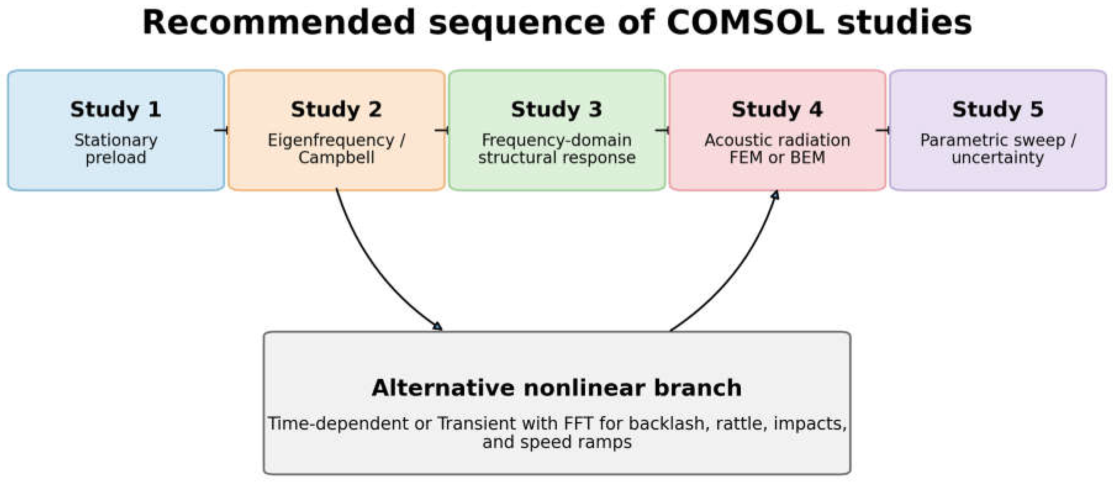
Figure 3. Recommended sequence of COMSOL studies, including the alternative nonlinear transient branch.

Figure 3. Recommended sequence of COMSOL studies, including the alternative nonlinear transient branch.

6.1. Study 1: Stationary Preload and Operating Equilibrium

The stationary study establishes gravity, torque, bearing preload, mount deformation, bolt pretension, and the loaded mesh state. It is also the natural point for verifying reaction-force balance. When nonlinear bearing or contact relations are used, load should be ramped with an auxiliary sweep or continuation strategy. The converged state is stored for subsequent prestressed modal or harmonic analysis.

6.2. Study 2: Eigenfrequency and Speed-Dependent Modal Analysis

The eigenfrequency study identifies shaft, housing, cover, and coupled rotor-stator modes. A speed sweep may be used to construct a Campbell diagram when gyroscopic or rotating-frame effects are significant. Modal classification should separate predominantly torsional, bending, bearing-seat, housing-panel, and global mounting modes. The target is not merely a list of frequencies; the mode shapes and modal participation at gear and bearing locations determine whether a resonance is relevant to the NVH path.

6.3. Study 3: Frequency-Domain Structural Response

Gear whine is most efficiently evaluated in the frequency domain. The load set consists of GMF harmonics, shaft orders, and sideband components derived from TE, mesh-force, or bearing-reaction spectra. A direct solution is suitable for small or medium models. Modal superposition or CMS is preferred for repeated sweeps when the response remains linear. The frequency grid must resolve narrow resonances and the order lines generated by the speed grid.

Two sweep strategies are useful. In a frequency sweep, the operating condition is fixed while frequency is varied. In an order-tracked operating sweep, frequency is defined from speed and tooth count so that every solution corresponds to a physical operating point. The second strategy is preferable when producing speed-frequency maps or comparing with run-up measurements.

6.4. Study 4: Acoustic Radiation

The structural surface velocity or acceleration is coupled to the acoustic field at the same frequencies. For one-way radiation, the structural solution can be reused as a prescribed normal velocity or acceleration. For fully coupled ASI, the acoustic pressure also loads the structure. One-way coupling is usually adequate for stiff metallic housings radiating into air, but the assumption should be checked when the surrounding fluid is dense, the structure is light, or an enclosed cavity strongly modifies the dynamics.

6.5. Alternative Transient Branch

Backlash, tooth impacts, intermittent contact, torque reversals, and rattle require a time-dependent model. The time step must resolve the highest relevant mesh harmonic and the shortest expected contact event. A speed ramp can be introduced through the prescribed angular velocity or torque. Spectra are obtained from a transient-with-FFT workflow or exported time histories. Windowing, sampling frequency, and record length must match the experimental processing chain.

6.6. Solver Recommendations

Table 6. Solver strategy by analysis type.

Problem type	Recommended approach	Main numerical risk
Linear modal screening	Eigenfrequency solver; simplified supports first, then calibrated supports	Rigid-body modes, overconstraint, inconsistent mass
Linear harmonic NVH	Direct solver for moderate size; modal/CMS reduction for repeated sweeps	Insufficient modal basis, poor damping calibration
Large coupled ASI FEM	Segregated or iterative strategy with suitable preconditioning	Memory use and convergence near dense modal regions
Exterior BEM radiation	Boundary-element acoustic formulation; direct or iterative solver depending size	Dense matrices and surface-mesh quality
Nonlinear backlash/rattle	Implicit time integration with gradual load initialization	Contact chatter, inconsistent initial conditions, too-large time steps
Large parametric campaign	Parametric Sweep with stored case identifiers; batch/cluster execution where available	Uncontrolled file size and incomplete metadata

Table 6. Solver strategy by analysis type.

Problem type	Recommended approach	Main numerical risk
Linear modal screening	Eigenfrequency solver; simplified supports first, then calibrated supports	Rigid-body modes, overconstraint, inconsistent mass
Linear harmonic NVH	Direct solver for moderate size; modal/CMS reduction for repeated sweeps	Insufficient modal basis, poor damping calibration
Large coupled ASI FEM	Segregated or iterative strategy with suitable preconditioning	Memory use and convergence near dense modal regions
Exterior BEM radiation	Boundary-element acoustic formulation; direct or iterative solver depending size	Dense matrices and surface-mesh quality
Nonlinear backlash/rattle	Implicit time integration with gradual load initialization	Contact chatter, inconsistent initial conditions, too-large time steps
Large parametric campaign	Parametric Sweep with stored case identifiers; batch/cluster execution where available	Uncontrolled file size and incomplete metadata

7. Variability-Aware Simulation Design

The purpose of variability analysis is not to create a large number of arbitrary runs. Each parameter must represent a physical source, a measurable tolerance, or a documented uncertainty. The parameter set is divided into manufacturing, assembly, operating, and degradation groups. This structure is aligned with simulation-ready gearbox NVH frameworks and allows the same input to be used in screening, sensitivity analysis, and stochastic propagation.

Table 7. Variability classes and their COMSOL representation.

Variability class	Representative parameters	Recommended model representation
Manufacturing	Profile and lead modification, pitch error, runout, tooth-to-tooth TE, housing wall thickness, material scatter	External LTCA or measured-data reduction; parameterized geometry only where remeshing is justified
Assembly	Bearing preload, clearance, center-distance error, shaft misalignment, mount stiffness, bolt preload	Bearing and joint parameters; local coordinate or foundation variations
Operating	Speed, torque, temperature, direction, lubricant state	Parametric sweep; temperature-dependent materials and bearing coefficients
Degradation	Wear-induced TE, stiffness loss, bearing clearance growth, joint loosening	State-indexed parameter sets or time-evolving functions

Table 7. Variability classes and their COMSOL representation.

Variability class	Representative parameters	Recommended model representation
Manufacturing	Profile and lead modification, pitch error, runout, tooth-to-tooth TE, housing wall thickness, material scatter	External LTCA or measured-data reduction; parameterized geometry only where remeshing is justified
Assembly	Bearing preload, clearance, center-distance error, shaft misalignment, mount stiffness, bolt preload	Bearing and joint parameters; local coordinate or foundation variations
Operating	Speed, torque, temperature, direction, lubricant state	Parametric sweep; temperature-dependent materials and bearing coefficients
Degradation	Wear-induced TE, stiffness loss, bearing clearance growth, joint loosening	State-indexed parameter sets or time-evolving functions

A staged design is recommended. First, perform one-factor sweeps to detect modeling mistakes and nonphysical trends. Second, use a screening design to rank variables. Third, apply a response-surface, Latin hypercube, or Monte Carlo design only to the influential subset. Correlated inputs should be preserved; for example, profile modification, TE amplitude, and mesh stiffness should not be sampled independently when they originate from the same measured flank geometry.

The minimum exported result vector for every case should contain the case ID, complete parameter vector, convergence status, reaction-force balance, selected modal frequencies, bearing-seat vibration, radiating-surface velocity, receiver SPL, sound power, and dominant order amplitudes. Failed cases must remain in the database with an error code rather than being silently discarded.

7.1. Automation with Parametric Sweep and Application Builder

COMSOL supports parametric studies through Parametric Sweep nodes and auxiliary sweeps. Auxiliary continuation is useful for nonlinear load ramping, while Parametric Sweep is preferable when geometry or multiple operating parameters are varied [1]. Application Builder can expose only the required inputs, enforce bounds, execute a predefined study sequence, and generate standardized reports [6]. For research reproducibility, the application layer should not hide the underlying model; it should formalize the run protocol and metadata capture.

• Read a parameter table with one row per simulation case.
• Validate units and allowed ranges before solving.
• Set the global case identifier and output directory.
• Run stationary, modal, structural frequency-domain, and acoustic studies in sequence.
• Evaluate predefined derived values and export tables without manual plot reading.
• Write a manifest containing model version, parameter file, timestamp, solver status, and output file names.

8. Numerical Verification and Experimental Validation

8.1. Numerical Verification

Verification asks whether the equations are being solved consistently, independent of whether the model represents the physical gearbox. The following checks are mandatory before experimental calibration.

Table 8. Numerical verification checks and recommended acceptance criteria.

Verification item	Procedure	Recommended acceptance criterion
Mass and inertia	Compare imported/simplified model with CAD or measured values.	Relative difference <= 1% for mass and <= 2% for principal inertias.
Static equilibrium	Sum applied and reaction forces/moments.	Force and moment residual <= 0.1% of the largest applied resultant.
Mesh convergence	Refine structural hot spots and acoustic wavelength mesh.	Selected eigenfrequencies change <= 1%; structural response <= 2%; SPL <= 1 dB.
Modal basis convergence	Increase retained modes or CMS basis.	Target-band displacement/velocity changes <= 1% after basis enrichment.
Frequency-grid convergence	Refine around resonances and order crossings.	Peak frequency changes <= 0.5% and peak level <= 1 dB after refinement.
Energy consistency	Compare input power, dissipated power, structural flux, and acoustic power.	Unexplained difference between input, dissipated, and radiated power <= 3%.
Interface force balance	Compare rotor bearing reactions and housing interface loads.	Equal-and-opposite interface resultants agree within 0.5%.
BEM/FEM radiation cross-check	Run selected frequencies with both formulations.	Receiver SPL agrees within 1.5 dB and radiated power within 10% at selected frequencies.

Table 8. Numerical verification checks and recommended acceptance criteria.

Verification item	Procedure	Recommended acceptance criterion
Mass and inertia	Compare imported/simplified model with CAD or measured values.	Relative difference <= 1% for mass and <= 2% for principal inertias.
Static equilibrium	Sum applied and reaction forces/moments.	Force and moment residual <= 0.1% of the largest applied resultant.
Mesh convergence	Refine structural hot spots and acoustic wavelength mesh.	Selected eigenfrequencies change <= 1%; structural response <= 2%; SPL <= 1 dB.
Modal basis convergence	Increase retained modes or CMS basis.	Target-band displacement/velocity changes <= 1% after basis enrichment.
Frequency-grid convergence	Refine around resonances and order crossings.	Peak frequency changes <= 0.5% and peak level <= 1 dB after refinement.
Energy consistency	Compare input power, dissipated power, structural flux, and acoustic power.	Unexplained difference between input, dissipated, and radiated power <= 3%.
Interface force balance	Compare rotor bearing reactions and housing interface loads.	Equal-and-opposite interface resultants agree within 0.5%.
BEM/FEM radiation cross-check	Run selected frequencies with both formulations.	Receiver SPL agrees within 1.5 dB and radiated power within 10% at selected frequencies.

8.2. Modal Validation

EMA provides the first experimental anchor because it isolates the structural transmission path before operational excitation is considered. Numerical and experimental frequencies are paired using mode-shape similarity and physical interpretation. The modal assurance criterion is

MAC(phi_a, phi_b) = |phi_a^H phi_b|^2 / [(phi_a^H phi_a)(phi_b^H phi_b)] (10)

Frequency error alone is insufficient: a high-frequency match with an incorrect mode shape can produce misleading confidence. The calibration sequence should prioritize boundary conditions and joint stiffness, then material properties, then damping. Parameters directly derived from manufacturing measurements should not be adjusted merely to improve a modal fit.

8.3. Operational Vibration and Acoustic Validation

Operational validation should use synchronized tachometer, vibration, and microphone data. The same speed, torque, temperature, mounting condition, and signal-processing settings must be used in simulation and test. Comparison quantities include housing acceleration at bearing seats and panel centers, complex FRFs where available, GMF order amplitude, sideband spacing, receiver SPL, directivity, and radiated sound power.

Table 9. Proposed experimental validation matrix.

Simulation output	Measurement	Comparison metric
Natural frequencies and mode shapes	Impact-hammer or shaker EMA	Frequency error and MAC
Bearing-seat FRF	Force-to-acceleration FRF	Magnitude/phase error and resonance alignment
Operational housing acceleration	Tachometer-synchronous accelerometers	Order amplitude and sideband structure
Receiver pressure spectrum	Microphones at matched coordinates	SPL error by frequency/order
Directivity	Microphone arc or array	Angular pattern and lobe orientation
Sound power	Measurement surface or intensity method	Band or order sound-power difference

Table 9. Proposed experimental validation matrix.

Simulation output	Measurement	Comparison metric
Natural frequencies and mode shapes	Impact-hammer or shaker EMA	Frequency error and MAC
Bearing-seat FRF	Force-to-acceleration FRF	Magnitude/phase error and resonance alignment
Operational housing acceleration	Tachometer-synchronous accelerometers	Order amplitude and sideband structure
Receiver pressure spectrum	Microphones at matched coordinates	SPL error by frequency/order
Directivity	Microphone arc or array	Angular pattern and lobe orientation
Sound power	Measurement surface or intensity method	Band or order sound-power difference

9. Worked Numerical Benchmark

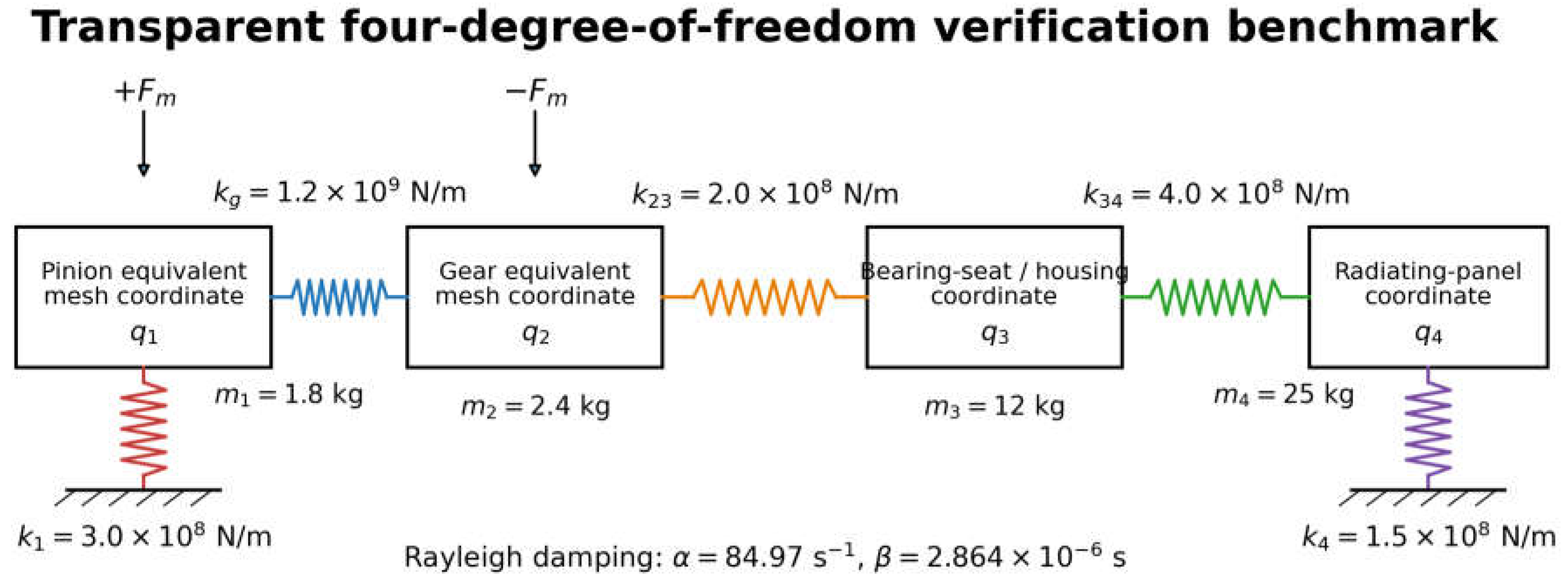
To make the workflow executable without relying on confidential gearbox geometry, a transparent four-degree-of-freedom benchmark was defined. It represents the line-of-action motion of the pinion and gear, the bearing-seat/housing coordinate, and one dominant radiating-panel coordinate. The benchmark is intentionally simple enough to solve directly from the matrix equations in Section 3, while every parameter can also be entered in COMSOL using the Lumped Mechanical System, Multibody Dynamics, or a reduced structural model. It is therefore an independent verification target rather than a substitute for a detailed finite-element gearbox.

9.1. Benchmark Definition and Reproducibility

The pinion has 23 teeth and the gear has 67 teeth. At the nominal pinion speed of 3000 rpm, the fundamental gear-mesh frequency is 1150 Hz. A peak line-of-action harmonic force of 100 N is applied as equal-and-opposite forces to the two gear coordinates. The four masses and five stiffnesses are listed in Table 10. Rayleigh damping was fitted to 2% modal damping at the first and third modes, giving alpha = 84.97 s^-1 and beta = 2.864 x 10^-6 s. These data fully determine the linear structural benchmark.

Figure 4. Four-degree-of-freedom benchmark used as an independent verification target for the COMSOL implementation.

Figure 4. Four-degree-of-freedom benchmark used as an independent verification target for the COMSOL implementation.

9.2. Modal Characteristics and Model-Reduction Verification

The undamped natural frequencies are 415.9, 1163.3, 1807.1, and 5737.3 Hz. The second mode lies only 1.16% above the nominal gear-mesh frequency and therefore controls the 3000-rpm response. Direct complex-frequency solution and mass-normalized modal superposition were compared at the nominal order. Retaining the first two modes gives a panel-displacement error of 0.233%; retaining the first three modes reduces the error to 0.0024%. At 2300 Hz, however, the three-mode error rises to 3.52%, demonstrating why a reduced basis must extend beyond the highest requested response frequency. This benchmark provides a practical acceptance test for a COMSOL modal or CMS model: the direct and reduced solutions should agree within the criteria in Table 8 before a large parameter campaign is started.

9.3. Speed Sweep and Structural Response

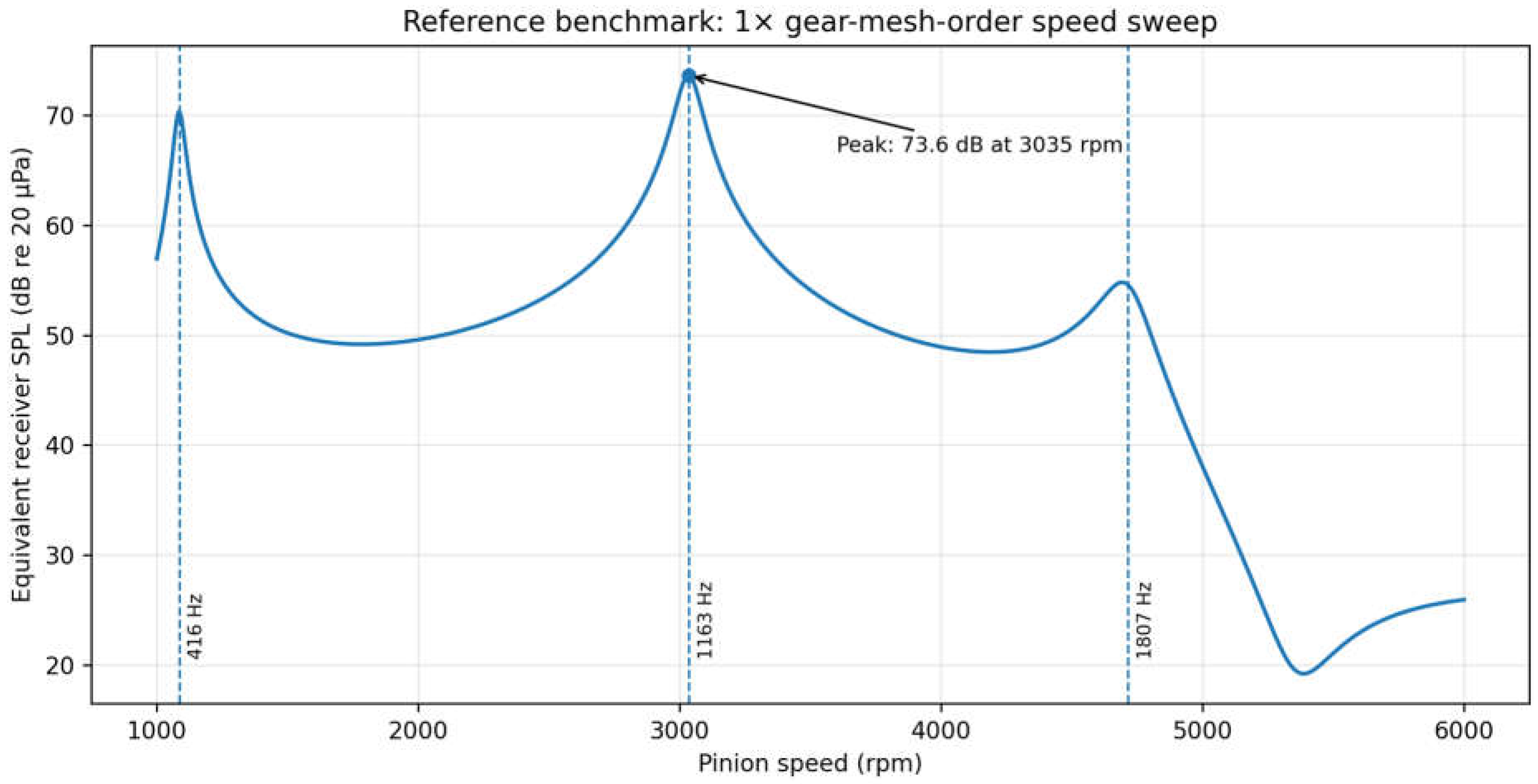
At 3000 rpm, the calculated panel displacement, velocity, and acceleration amplitudes are 1.391 x 10^-7 m, 1.005 x 10^-3 m/s, and 7.265 m/s^2, respectively. A pinion-speed sweep from 1000 to 6000 rpm was evaluated with the excitation locked to the fundamental gear-mesh order. The largest response occurs at 3035 rpm, where the order crosses the 1163.3-Hz mode. The result is a narrow resonance peak rather than a monotonic increase with speed. In the corresponding COMSOL model, this curve is obtained with a Parametric Sweep over rotational speed or with a Transient with FFT study when the run-up and modulation history must be preserved.

Figure 5. Equivalent receiver level for the 1 x gear-mesh-order speed sweep of the reference benchmark. Dashed lines indicate the first three structural modes.

Figure 5. Equivalent receiver level for the 1 x gear-mesh-order speed sweep of the reference benchmark. Dashed lines indicate the first three structural modes.

9.4. Acoustic Interpretation

For the benchmark only, the panel is treated as a compact baffled radiator to create a transparent acoustic cross-check. The root-mean-square pressure at distance r is estimated from p_rms = rho c k S |v_n| /(2 pi r sqrt(2)), where k is the acoustic wavenumber and v_n is the peak panel velocity. This approximation gives 71.95 dB re 20 microPa at 3000 rpm and 73.63 dB at the 3035-rpm resonance. These values are not presented as a replacement for the Acoustic-Solid Interaction or Pressure Acoustics, Boundary Elements solution. Their purpose is to detect unit, amplitude, phase, and postprocessing errors before the complete fluid domain is solved. In a detailed model, panel velocity is spatially distributed, radiation efficiency is mode dependent, and near-field and enclosure effects require FEM, BEM, or a coupled FEM-BEM formulation.

Table 11. Numerical results of the reference benchmark.

Result	Numerical value	Interpretation
Natural frequencies	415.9, 1163.3, 1807.1, 5737.3 Hz	The second mode governs the nominal GMF response.
Nominal GMF	1150 Hz at 3000 rpm	1.16% below the second mode.
Panel response at 3000 rpm	u = 1.391 x 10^-7 m; v = 1.005 x 10^-3 m/s; a = 7.265 m/s^2	Direct complex-frequency solution with 100 N peak mesh force.
Equivalent receiver level	71.95 dB at 3000 rpm	Transparent compact-radiator cross-check.
Speed-sweep maximum	73.63 dB at 3035 rpm (1163.4 Hz GMF)	Order crossing with the second structural mode.
Modal-superposition error	0.233% with 2 modes; 0.0024% with 3 modes at 1150 Hz	Confirms convergence of the reduced basis at the nominal order.
Monte Carlo statistics	Mean 68.21 dB; standard deviation 4.29 dB; median 68.46 dB	3000 samples at 3000 rpm.
95% variability interval	59.76-75.56 dB	Shows strong resonance-detuning asymmetry.

Table 11. Numerical results of the reference benchmark.

Result	Numerical value	Interpretation
Natural frequencies	415.9, 1163.3, 1807.1, 5737.3 Hz	The second mode governs the nominal GMF response.
Nominal GMF	1150 Hz at 3000 rpm	1.16% below the second mode.
Panel response at 3000 rpm	u = 1.391 x 10^-7 m; v = 1.005 x 10^-3 m/s; a = 7.265 m/s^2	Direct complex-frequency solution with 100 N peak mesh force.
Equivalent receiver level	71.95 dB at 3000 rpm	Transparent compact-radiator cross-check.
Speed-sweep maximum	73.63 dB at 3035 rpm (1163.4 Hz GMF)	Order crossing with the second structural mode.
Modal-superposition error	0.233% with 2 modes; 0.0024% with 3 modes at 1150 Hz	Confirms convergence of the reduced basis at the nominal order.
Monte Carlo statistics	Mean 68.21 dB; standard deviation 4.29 dB; median 68.46 dB	3000 samples at 3000 rpm.
95% variability interval	59.76-75.56 dB	Shows strong resonance-detuning asymmetry.

9.5. Variability and Sensitivity

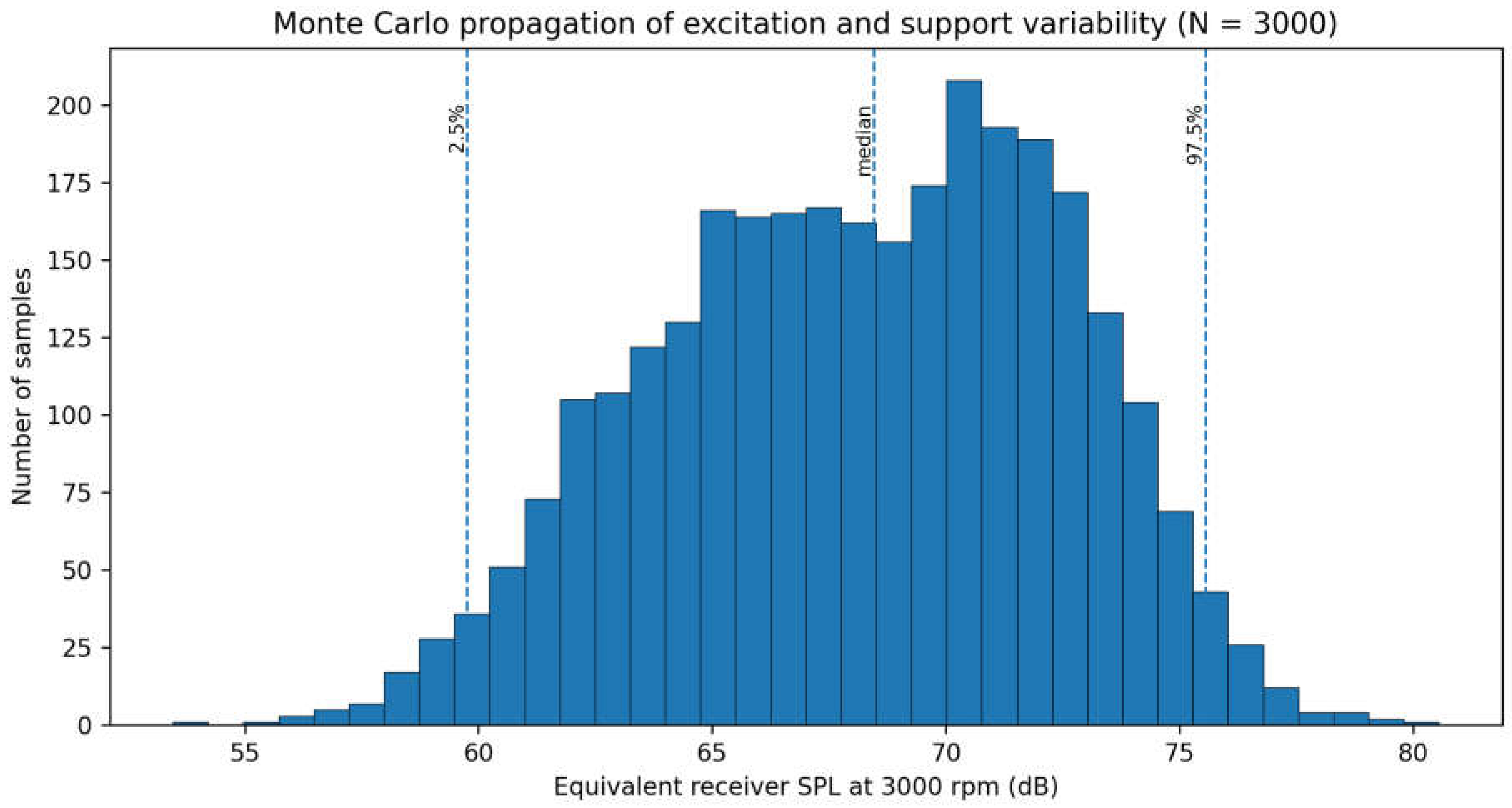
A 3000-sample Monte Carlo calculation was performed at 3000 rpm with independent normal variations in mesh-force amplitude (10% standard deviation), bearing-path stiffness k23 (10%), housing-to-panel stiffness k34 (8%), mount stiffness k4 (10%), and damping scale (20%). All samples were constrained to positive physical values. The resulting equivalent receiver level has a mean of 68.21 dB, a median of 68.46 dB, a standard deviation of 4.29 dB, and a central 95% interval of 59.76-75.56 dB. The distribution is asymmetric because small stiffness changes move the nominal operating point away from or toward the nearby mode.

Figure 6. Distribution of the equivalent receiver level after propagation of excitation, stiffness, mount, and damping variability.

Figure 6. Distribution of the equivalent receiver level after propagation of excitation, stiffness, mount, and damping variability.

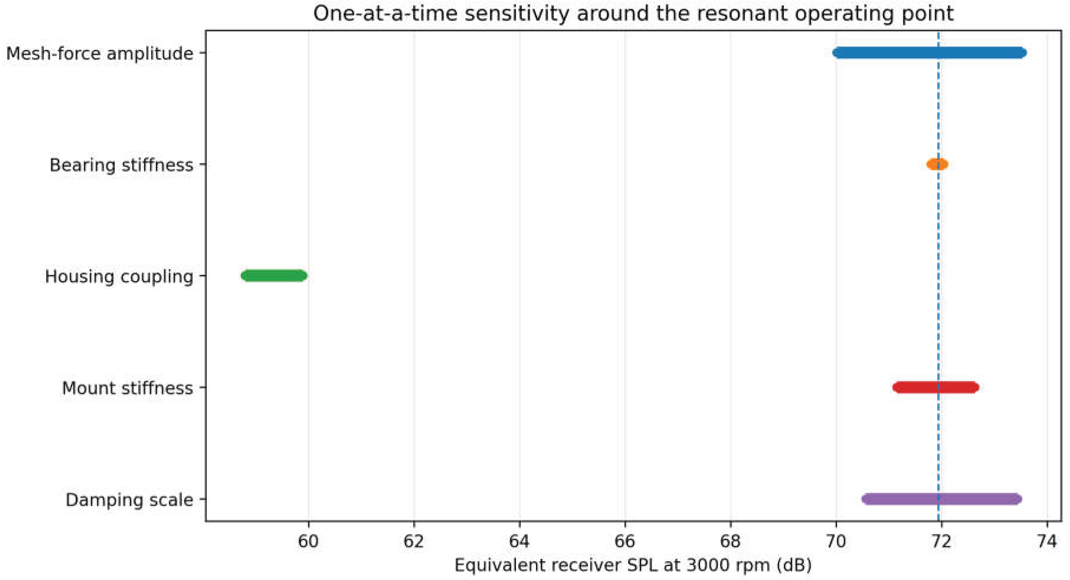
One-at-a-time variations confirm the resonance-dominated behavior. A +/-20% force change produces 70.01-73.53 dB, while a +/-25% damping-scale change produces 70.56-73.45 dB. The same +/-20% variation in k34 reduces the response to approximately 58.8-59.9 dB because both perturbations detune the nominal order from the second mode. Variations of k23 and k4 are smaller at this operating point. Spearman rank coefficients from the Monte Carlo set are -0.312 for k34, 0.198 for mesh-force amplitude, -0.165 for damping scale, 0.045 for k23, and -0.012 for k4. Consequently, the benchmark is transfer-path and resonance dominated rather than excitation dominated. This is precisely the distinction that a variability-aware COMSOL workflow must retain: reducing TE does not guarantee lower sound if the structural path moves closer to an order crossing.

Figure 7. One-at-a-time sensitivity ranges around the nominal 3000-rpm operating point. The dashed line is the nominal level.

Figure 7. One-at-a-time sensitivity ranges around the nominal 3000-rpm operating point. The dashed line is the nominal level.

10. Discussion

The main strength of the proposed workflow is the explicit separation between local tooth-contact information and system-level multiphysics propagation. COMSOL provides the documented mechanisms needed for the latter: gear-pair elasticity, TE, backlash and friction; rotor and bearing formulations; flexible structural models; and acoustic-structure coupling. Detailed LTCA and measured topography remain external inputs unless a custom contact formulation is developed. This division prevents the common error of assigning a level of tooth-contact fidelity that the system model does not actually contain.

The hierarchical strategy also addresses computational cost. A fully detailed solid-rotor and exterior-acoustic model is not necessary for every design question. Screening with a reduced-order drivetrain can identify critical orders and operating regions. The housing and acoustic models can then be refined only where the sensitivity is high. CMS and modal superposition are particularly valuable when hundreds of operating and variability cases are required.

The most important calibration parameter is often damping, but damping must not be used as a universal correction for geometry, support, or bearing errors. Structural damping should be identified from modal decay or FRFs; bearing and joint damping should be tied to the corresponding interfaces; and acoustic losses should be handled separately. A model that matches one receiver SPL through excessive global damping can still predict incorrect transfer paths and design trends.

The framework is deliberately compatible with manufacturing measurement data. CMM flank maps can be processed outside COMSOL to produce tooth-indexed TE, runout, and stiffness descriptors. Housing thickness measurements can update geometric parameters, while bearing preload or clearance can be represented directly. This allows the same COMSOL model to act as a common propagation layer for nominal, measured, and degraded states.

The numerical benchmark closes the methods chain without claiming validation of a proprietary gearbox. It demonstrates three conclusions that remain relevant in a detailed COMSOL model: the retained modal basis must extend beyond the response band; an order crossing can dominate the acoustic response; and manufacturing or assembly variability can reduce or increase noise primarily by detuning structural modes. The benchmark is intentionally low order, so its compact-radiator pressure estimate and lumped coordinates are verification devices rather than design predictions. Quantitative conclusions for a specific gearbox require its measured or verified geometry, bearing data, damping, excitation functions, and experimental correlation, but the implementation and acceptance criteria are complete and directly reusable.

10.1. Documented Limitations and Mitigation Measures

Table 12. Main limitations and mitigation measures.

Limitation	Consequence	Mitigation
No documented direct CMM flank-map import into the gear-pair contact law	Measured topography cannot be claimed as native tooth contact.	Reduce data externally to TE, stiffness, runout, phase, or equivalent force functions; document the reduction.
Gear-pair model is system level	Local tooth-root/contact stresses and microcontact may not be resolved.	Use LTCA/contact FE externally when those outputs are required.
Bearing data are uncertain and operating-point dependent	Resonance and transfer-path predictions can shift.	Use supplier/detailed-model coefficients, preload/clearance sweeps, and experimental identification.
Damping is difficult to predict	Peak amplitudes can be inaccurate even when modes are correct.	Calibrate by subsystem and frequency band; report the damping model.
High-frequency acoustic models are expensive	Large FEM domains or dense BEM matrices.	Use modal reduction, BEM for unbounded exterior radiation, and frequency-band partitioning.
Nonlinear transient runs are sensitive to initialization	Contact chatter and solver failure.	Use a stationary loaded state, gradual ramps, time-step convergence, and explicit failure logging.

Table 12. Main limitations and mitigation measures.

Limitation	Consequence	Mitigation
No documented direct CMM flank-map import into the gear-pair contact law	Measured topography cannot be claimed as native tooth contact.	Reduce data externally to TE, stiffness, runout, phase, or equivalent force functions; document the reduction.
Gear-pair model is system level	Local tooth-root/contact stresses and microcontact may not be resolved.	Use LTCA/contact FE externally when those outputs are required.
Bearing data are uncertain and operating-point dependent	Resonance and transfer-path predictions can shift.	Use supplier/detailed-model coefficients, preload/clearance sweeps, and experimental identification.
Damping is difficult to predict	Peak amplitudes can be inaccurate even when modes are correct.	Calibrate by subsystem and frequency band; report the damping model.
High-frequency acoustic models are expensive	Large FEM domains or dense BEM matrices.	Use modal reduction, BEM for unbounded exterior radiation, and frequency-band partitioning.
Nonlinear transient runs are sensitive to initialization	Contact chatter and solver failure.	Use a stationary loaded state, gradual ramps, time-step convergence, and explicit failure logging.

11. Conclusions

A reproducible COMSOL Multiphysics workflow has been formulated for gearbox vibroacoustic simulation from gear-mesh excitation to radiated sound. The approach combines external LTCA or measurement-derived excitation with COMSOL rotor, multibody, structural, and acoustic models. Baseline, recommended, and advanced fidelity levels match computational effort to the research question, while fixed verification criteria prevent large parametric campaigns from being built on an unconverged model.

The recommended implementation uses periodic TE and mesh-stiffness inputs, flexible shaft-bearing-housing coupling, prestressed modal and frequency-response studies, and FEM or BEM acoustic radiation. Nonlinear time-domain analysis is reserved for backlash, rattle, impacts, and speed transients. Parametric sweeps and application-level methods provide the execution layer for manufacturing, assembly, operating, and degradation variability.

The workflow establishes clear evidence boundaries. The reviewed COMSOL documentation supports gear elasticity, TE, backlash, friction, bearing and foundation models, flexible structures, and acoustic-structure interaction. Direct measured flank-topography contact is not documented and should therefore be introduced through a verified external reduction or a separately validated custom formulation. This distinction is essential for credible research claims.

The completed benchmark confirms the numerical logic of the workflow. At the nominal 1150-Hz gear-mesh order, three-mode superposition agrees with the direct solution within 0.003%, and the speed sweep identifies a 73.63-dB resonance peak at 3035 rpm. The 59.76-75.56-dB 95% variability interval shows that structural detuning can dominate the effect of excitation amplitude. The resulting article therefore provides both a complete COMSOL implementation protocol and a quantitative verification case that can be transferred to measured electric-vehicle gearbox models.

References

- COMSOL AB. Structural Mechanics Module User's Guide; Version 6.4; COMSOL AB.: Stockholm, Sweden, 2025. [Google Scholar]
- COMSOL AB. Rotordynamics Module User's Guide; Version 6.4; COMSOL AB.: Stockholm, Sweden, 2025. [Google Scholar]
- COMSOL AB. Multibody Dynamics Module User's Guide; Version 6.4; COMSOL AB.: Stockholm, Sweden, 2025. [Google Scholar]
- COMSOL AB. Acoustics Module User's Guide; Version 6.4; COMSOL AB.: Stockholm, Sweden, 2025. [Google Scholar]
- COMSOL AB. CAD Import Module User's Guide; Version 6.4; COMSOL AB.: Stockholm, Sweden, 2025. [Google Scholar]
- COMSOL AB. Introduction to Application Builder; Version 6.4; COMSOL AB.: Stockholm, Sweden, 2025. [Google Scholar]
- Smith, J.D. Gear Noise and Vibration, 2nd ed.; Marcel Dekker: New York, NY, USA, 2003. [Google Scholar]
- Litvin, F.L.; Fuentes, A. Gear Geometry and Applied Theory, 2nd ed.; Cambridge University Press: Cambridge, UK, 2004. [Google Scholar]
- Harris, T.A.; Kotzalas, M.N. Rolling Bearing Analysis, 5th ed.; CRC Press: Boca Raton, FL, USA, 2006. [Google Scholar]
- Fahy, F.; Gardonio, P. Sound and Structural Vibration: Radiation, Transmission and Response, 2nd ed.; Academic Press: Oxford, UK, 2007. [Google Scholar]
- Ewins, D.J. Modal Testing: Theory, Practice and Application, 2nd ed.; Research Studies Press: Baldock, UK, 2000. [Google Scholar]