Pricing Portfolios of Compute Capacity Contracts: Cross-Issuer Dependence and Segment Classification

1. Introduction

Multi-issuer compute capacity portfolios are quoted at institutional scale, the input-capacity counterpart to output-side inference-token futures (Xing [1]). Cleared compute-future indices reference multi-issuer deliverer pools rather than single names (e.g., CME Group and Silicon Data [2]; Intercontinental Exchange [3]; Architect Financial Technologies [4]); secondary-market reservation venues list contracts from heterogeneous issuers side-by-side (e.g., Compute Exchange [5]; Compute Exchange [6]); and multi-billion-dollar wholesale capacity transfers, syndicated infrastructure-backed financing, and lender collateral pools mix heterogeneous issuer types inside the same exposure book (e.g., xAI [7]; Core Scientific, Inc. [8]; Hut 8 Corp. [9]; Applied Digital Corporation [10]; CoreWeave, Inc. [11]; S&P Global Market Intelligence [12]). In each of these activities the relevant risk-management object is not a single contract $F_i^g(t,T)$ but a portfolio $\mathsf{\Pi }(t,T)={\sum }_i{w}_i{F}_i^g(t,T)$: the cleared indices settle a default-free, issuer-pooled rate, while marking or financing such a book turns on the joint distribution of issuer survival, recovery, and operational loss. One thesis organizes the paper: the cluster of co-exposed issuers is that book’s systematic, unhedgeable core—it does not diversify across names, a commodity index does not hedge it, and it closes only as credit instruments span it—so it must be priced, classified, and capital-held, not assumed away.

The single-issuer framework of Cao and Huang [13] prices each contract through a survival-conditional commodity forward coupled to a cause-conditional credit branch, with closed-form survival under affine intensity and a Föllmer–Schweizer local-risk-minimizing hedge. A portfolio is materially harder than a single name, because several cross-issuer dynamics absent from that model act at once: discrete common-shock clustering, a self-exciting funding-cascade contagion, cross-architecture substitution and its bistable lock-in, continuous factor co-movement, and an endogenous, wrong-way recovery. Each enters the price through a different term and in a different direction, so it is the joint distribution—not the marginals—that governs the basket. The paper’s main effort is to understand how: to fold all of these into a single tractable pricing equation and read off, for each dynamic, the term it drives, its direction, and whether a hedge removes it (§2, Table 1).

These dynamics sit against established but separate literatures. Factor-copula and common-factor credit models (Li [14]; Vasicek [15]; Duffie and Gârleanu [16]) capture continuous dependence but, being doubly stochastic, produce no simultaneous defaults; genuine clustering needs a discrete channel, which we build from Marshall–Olkin common shocks (Marshall and Olkin [17]; Lindskog and McNeil [18]) and self-exciting contagion (Errais et al. [19]), drawing on reinsurance retrocession and financial-network contagion (Eisenberg and Noe [20]; Glasserman and Young [21]; Cox and Pedersen [22])—a factor-contagion-with-Marshall–Olkin combination with a portfolio-credit precedent in Choe et al. [23], and default clustering studied dynamically by Karlis et al. [24] and Smug et al. [25]. Tradeability ranges from liquid tokens to non-transferable reservations within one book, so we price under the Föllmer–Schweizer / minimal-martingale tradition (Biagini and Cretarola [26]) through a three-mode segment map, the unhedgeable cross-issuer cluster risk falling into the residual; in Quantitative Finance the same incomplete-markets machinery prices liquid index options (Augustyniak et al. [27]) and, by utility indifference, options on illiquid assets through liquid proxies (Halperin and Itkin [28]), while emerging-asset hedging under basis risk has been treated for cryptocurrencies (Liu et al. [29]). Good-deal bounds themselves have priced incomplete-market and emerging-asset risk before—weather derivatives (Kanamura and Ōhashi [30]) and, in the closely related instantaneous-Sharpe-ratio form, longevity (Bayraktar et al. [31])—but, to our knowledge, neither within Quantitative Finance nor for a multi-issuer portfolio whose unhedgeable residual is cross-issuer cluster risk, the cell this paper occupies. Recent valuation-adjustment work flags portfolio-level cross-dependence as open (Sakuma [32]).

Our contribution answers that gap on the hedging side. Today’s market hedges the two outer layers—the delivery leg through the cleared futures, the single-name credit of the investment-grade nodes through CDS—but not the cross-issuer cluster core between them, which no traded index spans; we design the instruments that span it—a compute-CDS index, correlation tranches, a contagion-count swap, an architecture-share swap, and a proxy for the unspanned “keystone” counterparty (§8)—each laying off one channel. Hedging effectiveness is the no-arbitrage band each instrument removes, which a cluster-basis good-deal bound (Cochrane and Saá-Requejo [33]; Theorem 1) makes precise; the same bound fixes the irreducible floor—the loss carried by a node no contract references—so the market completes only up to its keystone. The construction holds for any basket of defaultable claims exposed to common shocks no traded index spans, with compute capacity the timely instance and two documented clusters—a realized 2022 mining-pivot cohort and the prospective NVIDIA–OpenAI–Oracle financing loop—calibrating the suite. It is integrative rather than foundational: affine intensities, Marshall–Olkin and self-exciting shocks, the minimal-martingale hedge, and the good-deal bound are established theory, composed on a new asset class into one closed-form pricer and the instrument suite it implies. Because the cluster instruments do not yet trade, effectiveness is model-implied, as befits a market still forming.

Our contribution answers that gap. When a basket’s tradeable hedges span only continuous and index risk, the cross-issuer cluster channel is wholly unhedgeable; when credit instruments span part of it, the residual contracts to a cluster-basis term that lower-bounds the no-arbitrage band and vanishes only in a fully-spanned, architecture-diversified limit (Theorem 1), the surviving correlation redistributed across tranches rather than hedged—a good-deal bound (Cochrane and Saá-Requejo [33]) and the formal counterpart of the correlation sensitivity that structured-finance pricing turns on (Coval et al. [34]). The bound holds for any basket of defaultable claims exposed to common shocks no traded index spans; compute capacity is the asset class that makes it concrete and timely. The affine construction that delivers it is closed-form throughout, carrying those dynamics in a single transform. The contribution is integrative rather than foundational: the ingredients—affine intensities, Marshall–Olkin and self-exciting cluster shocks, the minimal-martingale hedge, the good-deal bound—are established theory, and the work is to show that they compose, on a new and economically distinctive asset class, into one closed-form pricer whose unhedgeable residual carries an explicit, attained bound. Read in reverse, that bound is a design brief: it implies a suite of cluster-hedge instruments—an index, correlation tranches, a contagion-count swap, an architecture-share swap, and a keystone proxy—whose model-implied effectiveness is the band each removes (§8). The value is a tractable, calibratable framework for a market that postdates the tools it is built from—not a new result within any one of them, and not specific to compute. §2 sets up the pricing equation and the rest of the paper follows, with the two worked examples where it bites; results are stated with proof sketches.

2. The Joint Single-Period Setup

We work under a pricing measure $\tilde{\mathbb{Q}}$ equivalent to the physical measure $\mathbb{P}$, taken to be the minimal martingale measure of Föllmer and Schweizer [35] extended to defaultable claims by Biagini and Cretarola [26]. For a single issuer i supplying grade g, Cao and Huang [13] derives the forward price observed at t for delivery at T as

$$F_i^g(t,T)=S_i(t,T)G_i^g(t,T)e^{-{\mathsf{\Gamma }}_i(t,T)}+L_i^{\mathrm{recovery}}(t,T)-L_i^{\mathrm{op}}(t,T),$$

(1)

where $S_i$ is the survival probability of the terminal stopping time ${\tau }_i^{\mathrm{term}}$, $G_i^g$ is the survival-conditional commodity forward (with cost-of-carry exponential carrying the tradeability friction $u_i$ and the technology-depreciation drift ${\eta }_i^g$), $e^{-{\mathsf{\Gamma }}_i}$ the spot–credit correction (Cao and Huang [13] §6), $L_i^{\mathrm{recovery}}$ is the expected cause-conditional recovery (recovery-of-face-value reference), and $L_i^{\mathrm{op}}$ is the expected operational loss accumulated over the survival period. The present paper conditions on (1) as a per-issuer building block and extends to portfolios. Each $F_i^g$ is taken to be the joint spot–credit transform of Cao and Huang [13] §6, not the conditionally-independent product $S_i·G_i^g$: survival and delivered value co-move through the shared factors $X^{\mathrm{supply}}$ and $X^{\mathrm{macro}}$. That correction is second-order for investment-grade names but first-order in the high-intensity cluster regime priced here, where it no longer cancels across the delivery and recovery legs (§9); its cross-issuer extension is §5.

• The joint contract object.

A multi-issuer portfolio is the linear combination

$$\mathsf{\Pi }(t,T)={\displaystyle \sum _{i=1}^N}{w}_i{F}_i^g(t,T),$$

(2)

with ${\left\{w_i\right\}}_{i=1}^N$ a deterministic weight vector set by the basket product (equal, dollar, or notional weight). The joint claim $\mathsf{\Pi }(T,T)$ at delivery is not the sum of independent payoffs: cross-issuer dependence enters through several couplings developed in §4–§3, so pricing the basket requires the full joint distribution of $({\tau }_1^{\mathrm{term}},\dots ,{\tau }_N^{\mathrm{term}})$, of cause-conditional recoveries ${\left\{R_i^{\left(\kappa \right)}\right\}}_{i,\kappa }$, and of operational-loss compounders ${\left\{N_i^{\mathrm{op}}\right\}}_i$ under $\tilde{\mathbb{Q}}$.

The pricing equation itself does not change. Substituting the per-issuer building block (1) into (2) and annotating each term by the dynamics that drive it,

$$\mathsf{\Pi }(t,T)={\displaystyle \sum _{i=1}^N}{w}_i[\underset{\begin{array}{c}\mathrm{joint}\mathrm{survival}\text{:}\\ \mathrm{cluster}+\mathrm{contagion}\end{array}}{\underbrace{S_i}}\underset{\begin{array}{c}\mathrm{depreciation}\text{:}\\ \mathrm{obsolescence}+\mathrm{arch}.\end{array}}{\underbrace{G_i^g}}\underset{\begin{array}{c}\mathrm{spot}-\mathrm{credit}\\ \left(\mathrm{wrong}\text{-}\mathrm{way}\right)\end{array}}{\underbrace{e^{-{\mathsf{\Gamma }}_i}}}+\underset{\begin{array}{c}\mathrm{endogenous}\\ \mathrm{fire}-\mathrm{sale}\end{array}}{\underbrace{L_i^{\mathrm{recovery}}}}-\underset{\mathrm{op}.\mathrm{loss}}{\underbrace{L_i^{\mathrm{op}}}}],$$

(3)

the basket price keeps the single-issuer form unchanged. The contribution is not the equation but the content of its terms: five distinct dynamics, each previewed in §1, drive the values of $S_i$, $G_i^g$, and $R_i$, and one affine transform (§5) keeps all five in a single closed form. Table 1 maps each dynamic to the term it enters and the direction it pushes. The equation is the container; the five dynamics are the work, and the rest of the paper develops them in four steps: the dynamics that fill the terms (§§4–3), the affine transform that assembles them into the closed form (§5), the decomposition and hedging of the resulting risk down to the good-deal bound and the instrument suite it implies (§§6, 7 and 8), and two cluster examples calibrating the whole (§§9 and 10).

We organize issuers into a seven-type taxonomy (A–E2; Table A11), building on Cao and Huang [13], to structure the calibration; it carries type-conditional common-shock exposure loadings (§4) and the tradeability-based segment classification developed next.

• Segment classification by tradeability.

Tradeability varies sharply across these types, and with it the interpretation of the fair value (Cao and Huang [13] §3). The classification is operational: each row of Table A11 reflects how a participant in that segment should use the pricing output.

Definition 1

(Pricing mode). A compute capacity contract is classified into one of three pricing modes:

• (I) Arbitrage-enforced. Tradeability friction $u_i<\infty$, the spot underlying is tradeable, and a replicating strategy exists. Cash-and-carry bounds bind with small frictions, and observed mispricings invite arbitrage.
• (II) Minimal-martingale-measure (MMM) pricing. The spot underlying is not freely tradeable (forwards without secondary-market depth, or bilateral OTC without standardized transferability), so cash-and-carry chains only partially close. The contract is priced under the MMM $\tilde{\mathbb{Q}}$, with an unhedgeable residual borne by the holder that widens the no-arbitrage band (the Föllmer–Schweizer decomposition of §6.2).
• (III) Indicative pricing. $u_i\to \infty$ (non-transferable reservations, account-locked AI-lab credits) and the cash-and-carry chain breaks at the holding step. The per-issuer pricing equation (1) delivers what the contract would trade at under counterfactual tradeability; the output is useful for opportunity-cost benchmarking, internal valuation, and bilateral negotiation but not arbitrage-enforced.

Table A11, in Appendix A, instantiates this classification for the mid-2026 contract landscape—each issuer type mapped to its tradeability $u_i$ and pricing mode.

The practitioner deliverable is an explicit pricing-mode label on every contract: a risk officer marking mixed reservations knows which positions are arbitrage-disciplined, which need an MMM-band adjustment, and which are indicative-only, a distinction no single-issuer or segment-uniform treatment delivers.

3. Architecture: Substitution and Lock-in

The next two sections supply the five dynamics of Table 1—the two risk channels behind the price (3). We take the architecture channel first: the demand-side logic behind the delivered value $G_i^g$, and the slower, deeper driver of the two, since the workload-share dynamics developed here shape the collateral and demand on which the credit-side funding cascade of §4 rests. It has two parts: a slow substitution dynamic among competing hardware families, and the bistable lock-in that makes a tip out of an incumbent stack—not gradual drift—the systematic risk.

3.1. Substitution Dynamics

Cross-issuer dependence (§4) governs how issuers co-move and co-fail within an architecture family; cross-architecture substitution operates across families, on a slower timescale but with longer reach over multi-year tenors. Let $\mathcal{A}$ be the set of architecture families (NVIDIA datacenter GPU, Google TPU, AWS Trainium, Huawei Ascend, AMD Instinct, custom ASIC) and $s_a\left(t\right)\in [0,1]$ the workload share of $a\in \mathcal{A}$, with ${\sum }_a{s}_a\left(t\right)=1$. Shares evolve through a stochastic replicator dynamic with ecosystem increasing returns (Fisher and Pry [36]; Hofbauer and Sigmund [37]). Each family carries a fitness $f_a$ (a reallocation rate, units $1/$time) that rises with its own share $s_a$ at rate $\gamma \ge 0$, the strength of ecosystem increasing returns:

$$f_a\left(t\right)=\gamma s_a\left(t\right)+{\alpha }_a+{\beta }^{\mathrm{mig}}\left(\mathsf{\Delta }{\psi }_a\left(t\right)-{\phi }_a\right),$$

(4)

and the workload shares $s_a$ follow the replicator on the simplex,

$$d{s}_a=s_a\left(f_a\left(t\right)-\overline{f}\left(t\right)\right)dt,\overline{f}\left(t\right)={\sum }_{b\in \mathcal{A}}{s}_b{f}_b\left(t\right),$$

(5)

which preserves ${\sum }_a{s}_a=1$ by construction and, for two families (a against the field), reduces to the logistic $d{s}_a=s_a(1-s_a)(f_a-f_{a^{*}})dt$. The fitness collects the increasing-returns $\gamma$—the installed-base network externality of Katz and Shapiro [38], by which a family’s tooling, optimized kernels, and developer base grow with its own share; ${\alpha }_a$, an intrinsic, history-dependent asymmetry; ${\beta }^{\mathrm{mig}}>0$, the buyer migration sensitivity (the selection intensity, units $1/$time, converting a dimensionless merit gap into a reallocation rate); and two demand primitives.

Merit. ${\psi }_a\left(t\right)$ is the log perf-per-watt of family a’s current frontier, $\mathsf{\Delta }{\psi }_a\left(t\right)={\psi }_a\left(t\right)-{\psi }_{a^{*}}\left(t\right)$ its advantage over the dominant stack $a^{*}$. This is the cross-architecture face of the single-issuer perf-per-watt clock: Cao and Huang [13] §4 anchors within-family obsolescence to perf-per-watt against one exogenous frontier (the depth D); here that frontier is disaggregated into competing, family-specific frontiers, so the two depreciation channels share a clock—${\eta }_g^{\mathrm{life}}$ (aging below one’s own frontier, depth D) and ${\eta }_g^{\mathrm{arch}}$ (the gap between frontiers, $\mathsf{\Delta }{\psi }_a$).

Friction. ${\phi }_a\ge 0$ is the workload-porting cost onto family a (kernel re-tuning, precision and format changes, operational integration), a one-time cost amortized over the deployment horizon in perf-per-watt-equivalent units, with ${\phi }_{a^{*}}=0$ for the incumbent.

Frontier randomness. A competitor’s next-generation part may leapfrog on perf-per-watt, so the relative frontier is a $\tilde{\mathbb{Q}}$-diffusion,

$$d\mathsf{\Delta }{\psi }_a\left(t\right)={\mu }_{a}dt+{\sigma }_{a}d{W}_a^{\psi }\left(t\right),$$

(6)

making $(s_a,\mathsf{\Delta }{\psi }_a)$ a coupled system in which $s_a$ is random through $f_a$. Because no instrument pays on workload share, the cross-architecture share component is unhedgeable and orthogonal to the tradeable spot; the minimal martingale measure leaves its drift unchanged, so (5)–(6) hold under both $\mathbb{P}$ and $\tilde{\mathbb{Q}}$, and ${\eta }_g^{\mathrm{arch}}$ accordingly lands in the Föllmer–Schweizer residual $L^{FS}$ of §6.2.

Increasing returns and lock-in. Above a critical $\gamma$ the deterministic skeleton of (5) is bistable: an interior unstable equilibrium (a tipping point) separates basins toward $s_a\to 0$ (locked out) and $s_a\to 1$ (locked in), so the CUDA moat is an emergent lock-in basin (Arthur [39]), not an imposed drift, and the frontier shocks (6) carry the tail risk—a leapfrog large enough to cross the basin boundary tips the market. Empirically NVIDIA holds $\sim 80$–$85\%$ of training compute (from $\sim 95\%$ in 2020), compressing at $\sim 2.5$ pp/yr—a high-share basin eroding slowly, the signature of large $\gamma$. Equations (4)–(6) are a structural form, with $(\gamma ,{\alpha }_a,{\beta }^{\mathrm{mig}},{\phi }_a,{\mu }_a,{\sigma }_a)$ calibrated from observed migration rates and roadmap volatility.

• Integration into the pricing equation.

Substitution enters the per-issuer price (1) through both branches, introducing no new pricing primitive. Demand side: for a contract on a grade in family $a\left(i\right)$, anticipated share erosion of $a\left(i\right)$ over $[t,T]$ adds a cross-architecture component to the technology-depreciation drift in the cost-of-carry exponent of $G_i^g$,

$${\eta }_i^g(t,T)={\eta }_g^{\mathrm{life}}\left({\zeta }_t\right)+{\eta }_g^{\mathrm{arch}}(a\left(i\right);t,T),{\eta }_g^{\mathrm{arch}}(a\left(i\right);t,T)=max\left\{0,-{\displaystyle \frac{1}{T-t}}{\mathbb{E}}^{\tilde{\mathbb{Q}}}\left[ln\frac{s_{a\left(i\right)}\left(T\right)}{s_{a\left(i\right)}\left(t\right)}|{\mathcal{F}}_t\right]\right\},$$

(7)

the within-architecture lifecycle drift ${\eta }_g^{\mathrm{life}}\left({\zeta }_t\right)$ of Cao and Huang [13] §4 plus the average expected log-share decline of family $a\left(i\right)$ implied by (5): a losing family ($s_{a\left(i\right)}$ falling) raises ${\eta }_i^g$, depressing $G_i^g$ and hence $F_i^g$ by a tenor-growing migration premium. Supply side: for an issuer concentrated in a losing family, share erosion degrades revenue and hardware-collateral value, elevating the bankruptcy intensity ${\lambda }_i^{\left(\mathrm{bk}\right)}$ by an architecture-stress term increasing in family $a\left(i\right)$’s share loss, with loading ${\beta }_i^{\mathrm{arch}}\ge 0$ largest for single-stack neoclouds (Type B) and direct operators (Type E2) and near zero for diversified hyperscalers (Type C); the lower $S_i$ propagates to $F_i^g$. Cluster side: architecture stress also raises the funding-cascade arrival itself, not only the per-issuer hazard—a family losing share weakens the demand and collateral its same-family funding cluster rests on. Because that coupling lives inside the cluster’s arrival intensity, we fold it directly into the funding-cascade definition of §4, where it enters as the ${\theta }^{\mathrm{fc}}$ term of (15) and, through buffer erosion, arms the cascade’s branching-process criticality (the co-tipping of §4).

• Systematic exposure and tenor scope.

Because $s_a\left(t\right)$ is shared by every issuer on family a, it is a slow systematic driver: same-family issuers co-move through the common ${\eta }_g^{\mathrm{arch}}\left(a\left(i\right)\right)$ of (7) and through correlated ${\beta }_i^{\mathrm{arch}}$ loadings, so architecture concentration is a cross-sectional basket exposure complementary to the common-shock dependence of §4. Because the dynamics are bistable, this systematic risk is not gradual drift but the possibility of a tip out of the incumbent basin—the cross-architecture shock priced in the circular-financing cohort of §10. Within-architecture lifecycle dominates at the 1–3-year tenors currently traded; the cross-architecture term ${\eta }_g^{\mathrm{arch}}\left(a\left(i\right)\right)$ becomes material only beyond $\sim 4$-year tenors and for high-substitutability workloads (inference more portable than training).

3.2. Lock-in: Bifurcation, First-Passage Tipping, and Co-Tipping

The bistability asserted in §3.1 is not a metaphor: the replicator (5) is a one-dimensional gradient flow, so the moat, the tip, and the funding-cascade coupling are the equilibria, the saddle-node, and the cross-channel feedback of an explicit potential. Making it quantitative fixes the tenor at which architecture risk becomes material, supplies a calibrated tip-timing law for the cross-architecture shock priced in §10, and turns the wrong-way coupling ${\theta }^{\mathrm{fc}}$ of (15) into a co-tipping of two near-critical systems. The analysis stays subordinate to the pricing: every quantity below feeds the migration drift ${\eta }_g^{\mathrm{arch}}$ (7) and the good-deal band (33).

• The lock-in is a double-well.

Track the incumbent share $s\equiv s_{a^{*}}$ against the challenger field. The fitness gap (4) is $f_{a^{*}}-f_a=\gamma (2s-1)+m$ (using $\mathsf{\Delta }{\psi }_{a^{*}}={\phi }_{a^{*}}=0$ for the incumbent and $s_a=1-s$), where

$$m\equiv ({\alpha }_{a^{*}}-{\alpha }_a)-{\beta }^{\mathrm{mig}}\left(\mathsf{\Delta }{\psi }_a-{\phi }_a\right)$$

(8)

is the net incumbent advantage—intrinsic asymmetry less the challenger’s porting-adjusted merit edge. The two-family reduction of (5) is the logistic

$$ds=s(1-s)(f_{a^{*}}-f_a)dt=s(1-s)\left[\gamma (2s-1)+m\right]dt\equiv -U^{\prime }\left(s\right)dt,$$

a one-dimensional gradient flow (plus the frontier noise below). Here

$$U^{\prime }\left(s\right)=-s(1-s)\left[\gamma (2s-1)+m\right]=2\gamma s^3-(3\gamma -m)s^2-(m-\gamma )s,$$

which integrates to the quartic double-well potential

$$U\left(s\right)={\displaystyle \frac{\gamma }{2}}{s}^4-{\displaystyle \frac{3\gamma -m}{3}}{s}^3-{\displaystyle \frac{m-\gamma }{2}}{s}^2,$$

(9)

carrying wells at $s=0$ (locked out) and $s=1$ (locked in) separated by an unstable tipping barrier at

$$s^{*}=\frac{1}{2}-{\displaystyle \frac{m}{2\gamma }}.$$

(10)

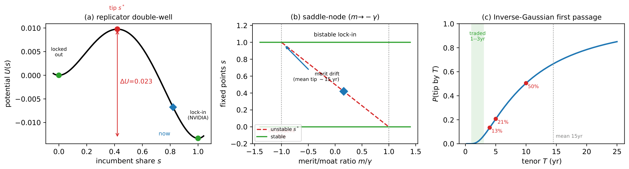
The CUDA moat of §3 is thus literally the basin of the $s=1$ well; the barrier lies below $\frac{1}{2}$ when the incumbent leads ($m>0$), and the incumbent at $s_0\approx 0.82$ sits well inside its basin (Figure 1(a)). Crucially m is not static: as the challenger frontier $\mathsf{\Delta }{\psi }_a$ closes (6), m falls, so the merit gap is a slow downward drift on the whole landscape that walks the operating point toward $s^{*}$.

• Two routes to a tip.

The barrier annihilates when $\left|m\right|=\gamma$: a saddle-node bifurcation at which the unstable point (10) merges with a well and the dynamics go monostable. A challenger whose porting-adjusted merit edge exceeds the lock-in strength, ${\beta }^{\mathrm{mig}}(\mathsf{\Delta }{\psi }_a-{\phi }_a)-({\alpha }_{a^{*}}-{\alpha }_a)>\gamma$, therefore tips the market deterministically—the slow-domino route. What makes the timing stochastic is not noise on the share—the replicator (5) carries none—but the frontier itself: (6) makes $\mathsf{\Delta }{\psi }_a$ a Brownian motion with drift, so through (8) the control parameter m is itself a drifting diffusion,

$$dm=-\dot{m}dt-{\sigma }_{m}d{W}_t,\dot{m}={\beta }^{\mathrm{mig}}{\mu }_a,{\sigma }_m={\beta }^{\mathrm{mig}}{\sigma }_a,$$

(11)

and the tip is the first passage of $m\left(t\right)$, from its current value $m_0$, to the saddle-node level $-\gamma$. For a drifting Brownian motion that first-passage time is Inverse-Gaussian,

$$T_{\mathrm{tip}}\sim \mathrm{IG}\left(\underset{\mathrm{mean}}{\underbrace{\frac{m_0+\gamma }{\dot{m}}}},\underset{\mathrm{shape}}{\underbrace{\frac{{(m_0+\gamma )}^2}{{\sigma }_m^2}}}\right),$$

(12)

with the drift $\dot{m}$ (structural catch-up) setting the mean and the frontier volatility ${\sigma }_m$ (an early leapfrog) setting the spread. This is the genuine two-route picture—a slow structural close and a sudden leapfrog—carried by a single law derived from the paper’s own (5)–(6), and it delivers exactly the object the pricing needs: the probability the family has tipped by the contract tenor, $\mathbb{P}(T_{\mathrm{tip}}\le T)$, on which ${\eta }_g^{\mathrm{arch}}\left(a\left(i\right)\right)$ (7) loads. (A bistable-potential view of default also appears in Smug et al. [25], but by Kramers escape of a coupling-driven barrier—additive noise on the health variable—rather than first passage of a drifting control parameter; here the randomness is the technology frontier, not the balance sheet.)

• Calibration.

Table 2 fixes the primitives, each tagged by provenance so the data-side refinement is a single re-fit rather than a re-derivation. The operating point $(s_0,\dot{s})$ and the cascade ratio $n_0$ are anchored to public figures cited in §3–§4; $\gamma$, the tipping share $s^{*}$, and the merit drift and volatility $(\dot{m},{\sigma }_m)$ are structural, the last two read from the perf-per-watt catch-up rate and generational dispersion scaled by the migration sensitivity ${\beta }^{\mathrm{mig}}$. They imply a net merit $m_0=\gamma (1-2s^{*})=0.08{\mathrm{yr}}^{-1}$ ($m_0/\gamma =0.16$, deep in the bistable regime), a barrier at $s^{*}=0.42$, and a distance to the saddle-node $m_0+\gamma =0.58$. The first-passage law (12) is then $\mathrm{IG}(\mathrm{mean}14.5\mathrm{yr},\mathrm{shape}15)$, a tip probability that climbs through the traded horizon,

$$\mathbb{P}(T_{\mathrm{tip}}\le T)=0.0\%,1.7\%,6.6\%,13.4\%,20.7\%\mathrm{at}T=1,2,3,4,5\mathrm{years}.$$

This was not an input: a calibration anchored to share and perf-per-watt data independently reproduces the tenor split asserted in §3— negligible across the 1–3-year traded tenors, material beyond $\sim 4$ years—and supplies the actual loading $\mathbb{P}(T_{\mathrm{tip}}\le T)$ that ${\eta }_g^{\mathrm{arch}}$ carries at each tenor. The drift/volatility split $(\dot{m},{\sigma }_m)$ is the structural part most in need of data: it decides whether the tip is a slow structural close (drift-dominated, narrow $T_{\mathrm{tip}}$) or a leapfrog risk (volatility-dominated, fat left tail). Figure 1 collects the potential, the saddle-node, and the first-passage curve.

Substitution and lock-in fix how architecture enters the delivered value $G_i^g$ and the per-issuer bankruptcy hazard, and shape the collateral the credit side rests on. We turn to that cross-issuer dependence next—and, with the architecture dynamics now in hand, to the buffer-erosion coupling that arms the funding cascade.

4. Cross-Issuer Dependence: Continuous Factors, Common Shocks, and Funding-Cascade Contagion

With the architecture channel of §3 in hand, this section supplies the three dynamics that sit inside the survival $S_i$ of (3)—the credit-side dependence among issuers. They arise from two channels: continuous co-movement, and a single discrete Marshall–Olkin common-shock structure whose firing rate takes two forms.

• Continuous. A common-factor state vector ${\mathbf{X}}_t=(X_t^{\mathrm{supply}},X_t^{\mathrm{macro}},X_t^{\mathrm{infra}},X_t^{\mathrm{reg}})$—a four-dimensional affine diffusion whose CIR and Vasicek coordinates carry supply and capacity-glut, macro credit-and-funding, physical-infrastructure, and regulatory stress—on which every issuer’s intensity loads; cross-issuer co-movement enters entirely through these shared loadings, the multi-name credit standard.
• Discrete: Marshall–Olkin common shocks. Counting processes $N^{\left(c\right)}$ (${\mathbb{N}}_0$-valued, unit jumps), $c\in \{\mathrm{infra},\mathrm{reg},\mathrm{fm},\mathrm{fc}\}$, each defaulting a loaded group of issuers at a single firing. All four share this group-fatal delivery and differ only in what drives the firing rate ${\nu }^{\left(c\right)}$: a shared external cause—${\mathbf{X}}_t$-affine—for infrastructure, regulatory, and force majeure (§4.2); contagion for the funding cascade ($c=\mathrm{fc}$), where a per-cluster self-exciting (Hawkes) state $J_k$—a piecewise-deterministic process, $+1$ at each member default, decay rate ${\kappa }^{\mathrm{fc}}$, gain ${\gamma }^{\mathrm{fc}}$, branching ratio $n={\gamma }^{\mathrm{fc}}/{\kappa }^{\mathrm{fc}}$—lifts ${\nu }^{\mathrm{fc}}$ as cluster members fail. In Table 1 both are sub-cases of the single Marshall–Olkin common shock—common-cause and contagion—not parallel dynamics.

Both are empirically forced, not modeling conveniences. Das et al. [40] reject conditional independence given observable factors for US corporate defaults—a doubly-stochastic law cannot reproduce the observed clustering, the discrete joint default the Marshall–Olkin common shocks deliver and diffusive factors miss. Azizpour et al. [41] then split that clustering into common factors and contagion, both significant—the two rate-forms above. The Marshall–Olkin structure delivers every discrete default; self-excitation is the contagion term, not a second delivery channel. The cause-indexed structure parallels the catastrophe-bond tradition of Cox and Pedersen [22] and the financial-network mechanisms of Eisenberg and Noe [20] and Glasserman and Young [21], in a tractable affine setting.

4.1. Continuous Channel

Cross-issuer dependence in the continuous channel enters entirely through the shared ${\mathbf{X}}_t$ loadings just named. The non-negative components ($X^{\mathrm{supply}},X^{\mathrm{infra}}$) follow CIR dynamics with the Feller positivity condition (Cox et al. [42]); the naturally-signed components ($X^{\mathrm{macro}},X^{\mathrm{reg}}$) follow Vasicek dynamics (Vasicek [43]). Idiosyncratic factors $Y_i^{\mathrm{op}},Y_i^{\mathrm{term}}$ follow issuer-specific CIR dynamics and are independent across issuers under $\tilde{\mathbb{Q}}$. Under conditional independence given ${\mathbf{X}}_t$, the cross-issuer intensity covariance factorizes as

$${cov}^{\tilde{\mathbb{Q}}}\left({\lambda }_i^{\mathrm{term}}\left(t\right),{\lambda }_j^{\mathrm{term}}\left(t\right)\right)={\tilde{\mathbf{a}}}_i^{\top }{Var}^{\tilde{\mathbb{Q}}}\left({\mathbf{X}}_t\right){\tilde{\mathbf{a}}}_j,$$

(13)

with ${\tilde{\mathbf{a}}}_i={\sum }_{\kappa }{\mathbf{a}}_i^{\left(\kappa \right)}$ the issuer-i aggregate common-factor loading, summed over the seven default causes of Cao and Huang [13],

$$\kappa \in \left\{\begin{array}{c}\mathrm{bankruptcy}\left(\mathrm{bk}\right),\mathrm{force}\mathrm{majeure}\left(\mathrm{fm}\right),\mathrm{regulatory}\mathrm{shutdown}\left(\mathrm{rs}\right),\mathrm{ecosystem}\mathrm{collapse}\left(\mathrm{ec}\right),\hfill \\ \mathrm{acquisition}·\mathrm{assumption}\left(\mathrm{aa}\right),\mathrm{acquisition}·\mathrm{repudiation}\left(\mathrm{ar}\right),\mathrm{verifiability}\mathrm{dispute}\left(\mathrm{vd}\right)\hfill \end{array}\right\}.$$

4.2. Marshall–Olkin Common Shocks

Every discrete joint default arrives this way: a single firing defaults a loaded group of issuers simultaneously, keeping the joint survival affine and closed-form (§5). The four families share this group-fatal delivery and split, by what drives the firing rate, into two sub-cases. Three—infrastructure, regulatory, and force majeure—fire on a shared external cause (${\mathbf{X}}_t$-affine: a datacenter-hub outage, an export-control round, a force-majeure event), and are developed in this subsection; the fourth, the funding cascade, is self-exciting, the contagion sub-case developed below:

• physical-infrastructure cascade ${\left\{N_m^{\mathrm{infra}}\right\}}_{m\in {\mathcal{M}}^{\mathrm{infra}}}$ indexed by E1 datacenter hub m, intensity affine in $X_t^{\mathrm{infra}}$;
• regulatory shock $N^{\mathrm{reg}}$ firing at announcement instants, intensity affine in $X_t^{\mathrm{reg}}$;
• force majeure $N^{\mathrm{fm}}$, approximately Poisson-constant;
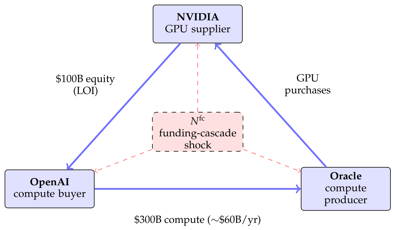
• financial-counterparty cluster (fc) ${\left\{N_k^{\mathrm{fc}}\right\}}_{k\in \mathcal{C}}$, indexed by cluster $k\in \mathcal{C}$, the AI-compute circular-financing loops cataloged in Appendix B (Table A12); its arrival intensity is instead self-exciting, developed below.

The infrastructure, regulatory, and force-majeure processes are independent of the Brownian factor dynamics and conditionally independent of one another given ${\mathbf{X}}_t$. Each shock loads its exposed issuers with a per-issuer probability ${\delta }_{i,\kappa }^{\left(c\right)}\in [0,1]$, the common-shock loading; Table 3 profiles the four families and these loadings.

• Cluster-shock contribution to cause-conditional default.

The common shocks act as fatal triggers. Each issuer carries the single-issuer idiosyncratic cause-$\kappa$ intensity ${\lambda }_i^{\left(\kappa \right),\sin \mathrm{gle}}\left(t\right)=a_{i,0}^{\left(\kappa \right)}+{\mathbf{a}}_i^{\left(\kappa \right)\top }{\mathbf{X}}_t+b_i^{\left(\kappa \right)}{Y}_i^{\mathrm{term}}\left(t\right)$ of Cao and Huang [13] §6; each firing of a common shock $N^{\left(c\right)}$ then triggers issuer i’s cause-$\kappa$ default independently with the loading ${\delta }_{i,\kappa }^{\left(c\right)}$. The cause-$\kappa$ survival is therefore

$$S_i^{\left(\kappa \right)}(t,T)={\mathbb{E}}^{\tilde{\mathbb{Q}}}\left[e^{-{\int }_t^T{\lambda }_i^{\left(\kappa \right),\sin \mathrm{gle}}\left(s\right)ds}\prod _{c\in {\mathcal{M}}^{\left(\kappa \right)}}{\left(1-{\delta }_{i,\kappa }^{\left(c\right)}\right)}^{N_T^{\left(c\right)}-N_t^{\left(c\right)}}|{\mathcal{F}}_t\right],$$

(14)

with ${\mathcal{M}}^{\left(\kappa \right)}$ the set of shocks affecting cause $\kappa$. An issuer with no exposure to shock source c has ${\delta }_{i,\kappa }^{\left(c\right)}=0$; a single firing defaults its loaded issuers simultaneously. This cause-to-shock map pairs regulatory shutdown with $N^{\mathrm{reg}}$, force majeure with $N^{\mathrm{fm}}$, bankruptcy and ecosystem collapse with the relevant $\left\{N_k^{\mathrm{fc}}\right\}$, and acquisition or verifiability dispute with ∅. The operational intensity ${\lambda }_i^{\mathrm{op}}$ loads on $\left\{N_m^{\mathrm{infra}}\right\}$ for cascading operational events.

• Contagion: the self-exciting funding cascade.

The funding cascade is the exception. There one node’s distress mechanically raises the next’s—a financier withdraws, a counterparty’s backlog impairs, shared collateral is dumped—so the cascade family alone carries endogenous feedback. Such feedback is modeled one of two canonical ways: resolve the balance-sheet clearing network default by default (the structural approach of Eisenberg and Noe [20] and Glasserman and Young [21]), or, reduced-form, let each default lift the arrival rate of the next—the self-exciting representation of contagion, canonical since Jarrow and Yu [44] and standard in affine credit (Errais et al. [19]; Aït-Sahalia et al. [45]). We take the reduced-form route: it delivers contagion while keeping the arrival intensity affine—so the joint survival stays closed-form (§5)—and compresses the cascade into a few interpretable parameters, the structural network re-entering only to calibrate them (the structural read $n_S$ below). Three ingredients make up its self-exciting core—an exogenous affine baseline, a self-exciting state $J_k$ that accumulates the cluster’s own defaults and forgets them at a fixed rate, and a gain turning that state into extra funding-shock hazard—and, because the architecture layer of §3 shapes the collateral the cluster rests on, a fourth term couples the two. For cluster k the arrival intensity ${\nu }_k^{\mathrm{fc}}$ is then the self-exciting affine point process of Errais et al. [19],

$${\nu }_k^{\mathrm{fc}}\left(t\right)={\nu }_{k,0}^{\mathrm{fc}}+{\mathbf{a}}_k^{\mathrm{fc}\top }{\mathbf{X}}_t+{\gamma }^{\mathrm{fc}}{J}_k\left(t\right)+{\theta }^{\mathrm{fc}}{\eta }_g^{\mathrm{arch}}(a\left(k\right);t),d{J}_k\left(t\right)=-{\kappa }^{\mathrm{fc}}{J}_k\left(t\right)dt+\sum _{i\in k}d{N}_i^{\mathrm{def}}\left(t\right),$$

(15)

where $N_i^{\mathrm{def}}$ counts issuer i’s default, ${\gamma }^{\mathrm{fc}}\ge 0$ is the contagion jump (the lift to the cluster’s funding-shock hazard per member default), and ${\kappa }^{\mathrm{fc}}>0$ its decay. The baseline ${\nu }_{k,0}^{\mathrm{fc}}+{\mathbf{a}}_k^{\mathrm{fc}\top }{\mathbf{X}}_t$ is affine in aggregate cluster revenue, cross-debt exposure, and equity-market signals; the ${\gamma }^{\mathrm{fc}}{J}_k$ term propagates a first failure to the survivors. The final term ${\theta }^{\mathrm{fc}}{\eta }_g^{\mathrm{arch}}\left(a\left(k\right)\right)$ is the architecture coupling: $a\left(k\right)$ is the cluster’s dominant family, ${\eta }_g^{\mathrm{arch}}\left(a\left(k\right)\right)$ its migration drift (7) from §3, and ${\theta }^{\mathrm{fc}}\ge 0$ the coupling strength, so a tip out of the family’s basin both depreciates the delivered good (via ${\eta }_g^{\mathrm{arch}}$) and arms the cluster’s cascade (via ${\theta }^{\mathrm{fc}}$)—the wrong-way axis of §10 made structural (its decoupling and buffer-erosion limits are anchored with the co-tipping below). Two limits anchor it: at ${\gamma }^{\mathrm{fc}}=0$ the channel collapses to a pure common shock (and to the common-shock families above), while for a singleton cluster $J_k$ has no surviving member to act on, so self-excitation is a genuine $\left|k\right|\ge 2$ phenomenon—absent, in particular, in the single-issuer reduction of Cao and Huang [13].

• Calibrating the contagion gain.

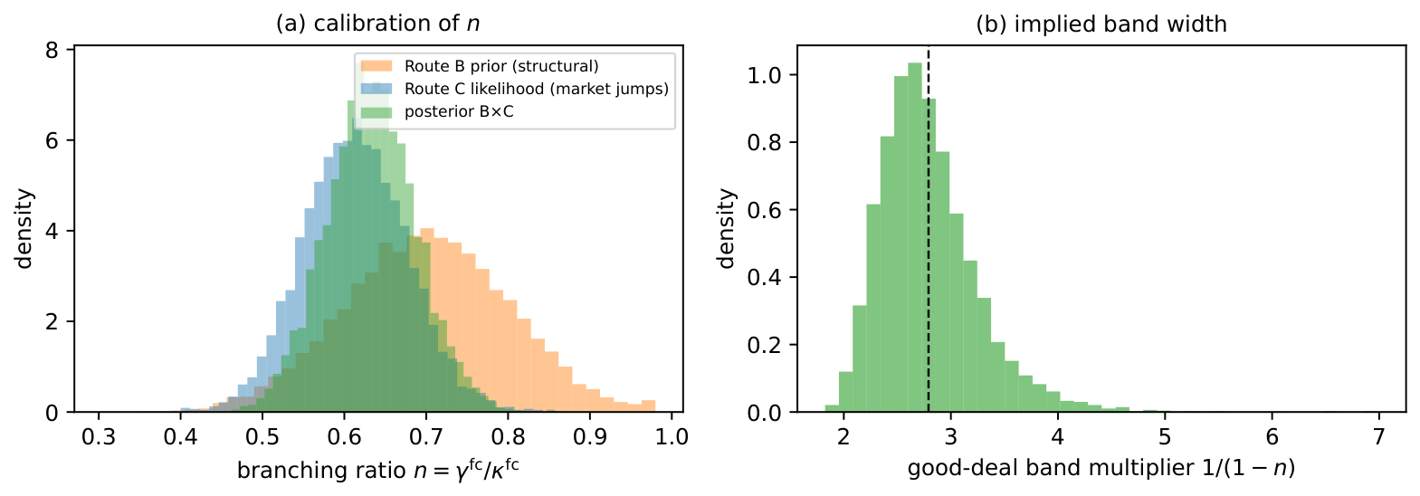
The branching ratio $n={\gamma }^{\mathrm{fc}}/{\kappa }^{\mathrm{fc}}$—the kernel mass ${\int }_0^{\infty }{\gamma }^{\mathrm{fc}}{e}^{-{\kappa }^{\mathrm{fc}}t}dt$ of (15), equivalently the mean offspring of its Hawkes–Oakes branching representation (Hawkes [46]; Hawkes and Oakes [47])—is the expected number of direct knock-on defaults one cluster default triggers. It lies below one not by definition but by stability: the self-exciting process is stationary exactly when this branching is subcritical, $n\in [0,1)$, so one exogenous default seeds a cascade finite in mean, of total size $1/(1-n)$, whereas $n\ge 1$ is explosive. Two independent reads calibrate it from today’s data.1 The structural read $n_S$ is the expected knock-on count of the directed exposure network,

$$n_S={\mathbb{E}}_i\left[\#\{j:\mathrm{LGD}·E_{j\leftarrow i}>B_j\}\right],{\kappa }^{\mathrm{fc}}=1/{\overline{\tau }}_{\mathrm{cad}},$$

(16)

with $E_{j\leftarrow i}$ the exposure of j to i, $\mathrm{LGD}$ the loss given default, $B_j$ the loss-absorbing buffer, the expectation over a uniformly-random first defaulter $i\in k$, and ${\overline{\tau }}_{\mathrm{cad}}$ the mean contractual interval (payment, maturity, refinancing) that sets the decay; built from the same exposure-to-buffer ratios $E_i/B_i$ that pin the loadings ${\delta }_i$ (§9; Eisenberg and Noe [20]; Glasserman and Young [21]; Boissay and Gropp [48]), it rises with loop tightness and is near-critical for a fully circular structure. The market-implied read $n_M$ instead fits (15) (Errais et al. [19]) by maximum likelihood to the detected jump times $\left\{t_m\right\}$ of the cluster names’ listed equity returns and credit spreads,

$$\begin{array}{cc}\hfill ({\widehat{\gamma }}^{\mathrm{fc}},{\widehat{\kappa }}^{\mathrm{fc}})& =arg{max}_{{\gamma }^{\mathrm{fc}},{\kappa }^{\mathrm{fc}}}\left[{\sum }_{m}log{\nu }_k^{\mathrm{fc}}\left(t_m\right)-{\int }_0^T{\nu }_k^{\mathrm{fc}}\left(s\right)ds\right],\hfill \\ \hfill n_M& ={\widehat{\gamma }}^{\mathrm{fc}}/{\widehat{\kappa }}^{\mathrm{fc}},\hfill \end{array}$$

(17)

abundant high-frequency data needing no default, its lead–lag structure identifying the direction of propagation. Because the two draw on disjoint inputs—balance-sheet structure versus market prices—they co-verify: agreement validates the contagion specification, while the gap $n_S-n_M$ is itself the diagnostic. A positive gap $n_S>n_M$ (structure implying more contagion than the market prices) is unpriced loop circularity—the structured-finance-style under-pricing the band of §7 measures; a negative gap $n_S<n_M$ flags exposure the balance sheet omits (off-balance-sheet vehicles) or sentiment overshoot. We therefore do not average them but treat the structural read as a prior the market read updates,

$$\begin{array}{cc}\hfill & n\sim \mathcal{N}(n_S,{\sigma }_S^2),n_M\mid n\sim \mathcal{N}(n,{\sigma }_M^2)⟹n\mid n_M\sim \mathcal{N}(\widehat{n},{\widehat{\sigma }}^2),\hfill \\ \hfill & \widehat{n}={\displaystyle \frac{n_S{\sigma }_S^{-2}+n_M{\sigma }_M^{-2}}{{\sigma }_S^{-2}+{\sigma }_M^{-2}}},{\widehat{\sigma }}^{-2}={\sigma }_S^{-2}+{\sigma }_M^{-2}.\hfill \end{array}$$

(18)

Where they agree the posterior sharpens, $\widehat{\sigma }<min({\sigma }_S,{\sigma }_M)$; where they diverge, the standardized wedge $z=(n_S-n_M)/\sqrt{{\sigma }_S^2+{\sigma }_M^2}$ is the result—the shift between what the loop structurally is and what the market has priced, not a forecast of cascade. For the 2025–26 cluster (§10) the documented circularity puts $n_S$ high while a young market plausibly prices $n_M$ lower, so the expected reading is a positive wedge $z>0$, with the band (33) widening by $1/(1-\widehat{n})$ at the posterior $\widehat{n}$ the data support.

• Co-tipping: the architecture tip arms the cascade.

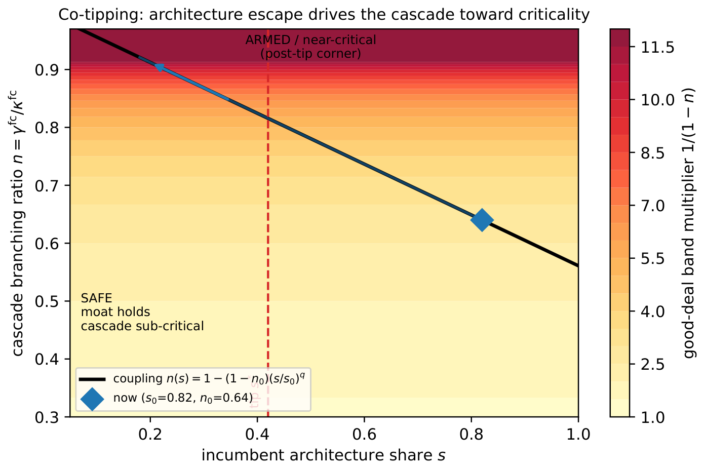
The two near-critical systems are coupled, and not only through the intercept shift ${\theta }^{\mathrm{fc}}$ of (15). A family losing share weakens the demand and collateral the same-family funding cluster rests on (§3), lifting the exposure-to-buffer ratios $E_j/B_j$ that set the structural knock-on count (16) and hence the branching ratio $n={\gamma }^{\mathrm{fc}}/{\kappa }^{\mathrm{fc}}$ itself. Writing the buffer erosion as $n\left(s\right)=1-(1-n_0){(s/s_0)}^q$—so $n=n_0$ at the current share and $n\to 1$ as the family is locked out—the architecture saddle-node (10) feeds the cascade’s branching-process criticality at $n\to 1$, where the good-deal multiplier $1/(1-n)$ of (33) diverges. A tip from $s_0=0.82$ to $s^{*}=0.42$ lifts n from $0.64$ to $0.82$, widening the band from $2.8$ to $5.4$; a deeper lock-out toward $s=0.20$ drives $n\to 0.91$ and the band past 11. Figure 2 plots this $(s,n)$ phase plane: the operating point sits in the safe corner, but the coupling curve carries it into the near-critical region as the share falls. This is the co-tipping a single double-well cannot express—the architecture tip of (12) does not merely depreciate the delivered good through ${\eta }_g^{\mathrm{arch}}$, it drives a second system toward its own critical point, and the band prices both at once.

Two limits anchor the construction. At ${\theta }^{\mathrm{fc}}=0$ and $q\to \infty$ (buffers insensitive to share) the channels decouple and the conditional independence of §6 is exact; and in the single-issuer reduction of Cao and Huang [13] there is no surviving member for $J_k$ to act on ($n\equiv 0$) and no cross-family share to tip, so Figure 1 and Figure 2 collapse to a point—the dynamics are genuinely portfolio-level. The lone illustrative knob is the buffer–share elasticity q; the qualitative blow-out is robust to it, the magnitude awaiting the empirical $E_j/B_j$-to-share elasticity of Table 2.

This completes the five dynamics: architecture enters the price twice—depreciating the delivered value, and, through buffer erosion, arming the funding cascade. The next section assembles them all into one closed-form price.

5. Joint Affine Intensity and Closed-Form Joint Survival

The dynamics of §§3 and 4 now become the single closed form that (3) promised: one affine transform prices them all. With the common-shock default construction (14), the joint state

$${\mathbf{Z}}_t:=\left({\mathbf{X}}_t,{\{Y_i^{\mathrm{op}},Y_i^{\mathrm{term}},Y_i^P\}}_{i=1}^N,{\zeta }_t,{\left\{N_t^{\left(c\right)}\right\}}_c,{\left\{J_k\right\}}_{k\in \mathcal{C}}\right),Y_i^P:=ln{P}_i^{g,\mathrm{spot}},$$

is an affine jump-diffusion in the sense of Duffie et al. [49]: the idiosyncratic cause-conditional intensities are affine in ${\mathbf{Z}}_t$, the common shocks are jump-to-default triggers with ${\mathbf{X}}_t$-affine arrival intensity, and the funding-cascade arrival is affine in the self-exciting state $J_k$, which jumps at cluster defaults and decays (15)—an affine point process (Errais et al. [19]). By Proposition 1 of Duffie et al. [49] the joint Laplace transform retains its exponential-affine form, the Riccati system gaining the common-shock and self-excitation survival terms below.

• The architecture channel and conditional affinity.

The cross-architecture state ${\mathsf{\Theta }}_t:=(\left\{s_a\left(t\right)\right\},\left\{\mathsf{\Delta }{\psi }_a\left(t\right)\right\})$ of §3 sits outside this affine core: the bankruptcy intensity loads on the nonlinear share through ${\beta }_i^{\mathrm{arch}}$, so the intensities are not affine in ${\mathsf{\Theta }}_t$. We exploit the timescale separation—architecture evolves on the multi-year clock of §3, an order of magnitude slower than the credit and lifecycle dynamics—and freeze ${\mathsf{\Theta }}_t$ over the credit window. Conditional on ${\mathsf{\Theta }}_t$, the architecture-stress term is a constant shift of the intensity intercept, the intensities are affine in ${\mathbf{Z}}_t$, and the joint survival below is closed-form; the unconditional price integrates that closed form over the slow, low-dimensional law of $\mathsf{\Theta }$ (a one- or two-factor outer expectation). The construction is therefore closed-form on the affine credit core and numerical only on the slow architecture layer.

• Joint survival probability.

For two issuers $i,j$, the joint survival probability admits the exponential-affine closed form

$${\mathbb{P}}^{\tilde{\mathbb{Q}}}\left[{\tau }_i^{\mathrm{term}}>T,{\tau }_j^{\mathrm{term}}>T|{\mathcal{F}}_t\right]=exp\left(A_{ij}^S\left(\tau \right)+{\mathbf{B}}_{ij}^S{\left(\tau \right)}^{\top }{\mathbf{Z}}_t\right),\tau =T-t,$$

(19)

with $A_{ij}^S\left(0\right)=0,{\mathbf{B}}_{ij}^S\left(0\right)=\mathbf{0}$. The Riccati system reads

$$\begin{array}{cc}\hfill {\displaystyle \frac{d{A}_{ij}^S}{d\tau }}& =-({\tilde{a}}_{i,0}+{\tilde{a}}_{j,0})+{\mathbf{B}}_{ij}^{S\top }\left(\mathbf{K}\theta \right)+\frac{1}{2}{\mathbf{B}}_{ij}^{S\top }{\mathsf{\Sigma }}_0{\mathbf{B}}_{ij}^S\hfill \\ \hfill & +\sum _c\left((1-{\delta }_{i,\kappa }^{\left(c\right)})(1-{\delta }_{j,\kappa }^{\left(c\right)})-1\right){\nu }^{\left(c\right)}\left(t\right),\hfill \\ \hfill {\displaystyle \frac{d{\mathbf{B}}_{ij}^S}{d\tau }}& =-({\tilde{\mathbf{a}}}_i+{\tilde{\mathbf{a}}}_j)-{\mathbf{K}}^{\top }{\mathbf{B}}_{ij}^S+\frac{1}{2}{\mathbf{B}}_{ij}^{S\top }{\mathsf{\Sigma }}_1{\mathbf{B}}_{ij}^S,\hfill \end{array}$$

(20)

where ${\delta }_{i,\kappa }^{\left(c\right)}\in [0,1]$ is issuer i’s cause-$\kappa$ default probability per firing of shock c, ${\nu }^{\left(c\right)}\left(t\right)$ is the affine common-shock arrival intensity, and the last term in $d{A}_{ij}^S/d\tau$ is the common-shock survival contribution. For the funding-cascade family the arrival ${\nu }_k^{\mathrm{fc}}\left(t\right)$ is itself state-dependent through the self-exciting term ${\gamma }^{\mathrm{fc}}{J}_k\left(t\right)$ of (15): $J_k$ enters ${\mathbf{Z}}_t$ as an affine coordinate whose generalized-Riccati equation carries the decay $-{\kappa }^{\mathrm{fc}}$ and the per-default jump, so the cascade is priced within the same exponential-affine transform (Errais et al. [19]) and (20) gains the corresponding $J_k$ component. The $(\mathbf{K},\theta ,{\mathsf{\Sigma }}_0,{\mathsf{\Sigma }}_1)$ parameters extend the single-issuer specification of Cao and Huang [13] §6 to the joint state ${\mathbf{Z}}_t$. $L_i^{\mathrm{op}},L_i^{\mathrm{recovery}}$ admit parallel jump-extended exponential-affine forms via the same machinery.

• Joint pricing.

Substituting (19) into the per-issuer pricing equation (1) for each i yields the joint distribution of ${\left\{F_i^g(t,T)\right\}}_{i=1}^N$ as a tractable function of ${\mathbf{Z}}_t$, the commodity forwards $\left\{G_i^g\right\}$, and the Riccati coefficients. Portfolio prices $\mathsf{\Pi }(t,T)$ from (2) inherit the same tractability through linearity of the expectation.

• Spot–credit correlation across the basket.

The joint state now carries each issuer’s log-spot $Y_i^P$, so the basket delivery stream is the joint spot–credit transform of Cao and Huang [13] §6 extended to ${\mathbf{Z}}_t$: it solves the analogous affine transform under the delivery terminal condition ${\sum }_i{w}_i{\mathbf{e}}_{Y_i^P}$ in place of the survival condition ${\mathbf{B}}_{ij}^S\left(0\right)=\mathbf{0}$, with the spot–credit covariance entering through the off-diagonal blocks ${\mathsf{\Sigma }}_{P_i,\nu }$ (issuer-i spot with factor $\nu$) and ${\mathsf{\Sigma }}_{P_i,P_j}$ (cross-issuer spot) of ${\mathsf{\Sigma }}_0$. The conditionally-independent product is the corner ${\mathsf{\Sigma }}_{P_i,·}=0$; because the common shocks of §4 raise the effective hazard, this spot–credit covariance, negligible for a diversified investment-grade basket, becomes first-order for the concentrated cohort of §9.

Remark 1

(Limiting cases). With zero common-shock loadings ${\delta }_{i,\kappa }^{\left(c\right)}=0$ and no funding-cascade self-excitation (${\gamma }^{\mathit{fc}}=0$, or singleton clusters), the common-shock and self-exciting terms in (20) vanish and (19) reduces to the product ${\mathbb{P}}^{\tilde{\mathbb{Q}}}\left[{\tau }_i^{\mathit{term}}>T|{\mathcal{F}}_t\right]·{\mathbb{P}}^{\tilde{\mathbb{Q}}}\left[{\tau }_j^{\mathit{term}}>T|{\mathcal{F}}_t\right]$ conditional on the common-factor path ${\mathbf{X}}_{[t,T]}$; the marginals coincide with the single-issuer closed form $S_i(t,T)=exp(A_i^S\left(\tau \right)+{\mathbf{B}}_i^S{\left(\tau \right)}^{\top }{\mathbf{Z}}_{i,t})$ of Cao and Huang [13], equation (6.2). Dependence then operates entirely through the continuous channel (13). Conversely, with common-shock loadings non-zero but ${\mathbf{X}}_t$ deterministic, dependence operates entirely through the discrete channel.

Remark 2

(Bindable versus shiftable exposure). The baseline treats ${\delta }_{i,\kappa }^{\left(c\right)}$ as bindable in the short term (an issuer cannot dodge a hub failure by shifting workloads mid-disruption). A refinement scales it by a binding-share $s_{i,c}\in [0,1]$, below one for portable-workload issuers (e.g., Type A protocols), calibrated from operator disclosures.

• Endogenous fire-sale recovery.

The baseline treats the cause-$\kappa$ recovery $R_i^{\left(\kappa \right)}$ as an exogenous draw. In a cluster, however, the loaded issuers default simultaneously and force a shared, increasingly single-use hardware fleet into the same thin secondary market at once, so the realized recovery is lowest in precisely the states where many names fire together. We endogenize it as a decreasing function of the contemporaneous common-shock count,

$$R_i^{\left(\kappa \right)}\left(\left\{N_T^{\left(c\right)}\right\}\right)={\underline{R}}_i^{\left(\kappa \right)}+\left(R_i^{\left(\kappa \right),0}-{\underline{R}}_i^{\left(\kappa \right)}\right)exp\left(-{\gamma }_i^{\mathrm{fs}}\sum _{c\in {\mathcal{M}}^{\left(\kappa \right)}}{N}_T^{\left(c\right)}\right),$$

(21)

interpolating between the no-cascade level $R_i^{\left(\kappa \right),0}$—the exogenous single-issuer recovery of Cao and Huang [13]—and a fire-sale floor ${\underline{R}}_i^{\left(\kappa \right)}$, with fire-sale sensitivity ${\gamma }_i^{\mathrm{fs}}\ge 0$ and ${\mathcal{M}}^{\left(\kappa \right)}$ the cause-$\kappa$ shock set of (14). Because the recovery is exponential in the shock counts, the recovery leg stays within the extended affine transform: the per-firing tilt $e^{-{\gamma }_i^{\mathrm{fs}}}$ enters the recovery-leg Riccati exactly as the survival weight $(1-{\delta }_{i,\kappa }^{\left(c\right)})$ enters (20), so $L_i^{\mathrm{recovery}}$ keeps its closed form on the affine credit core (the tilt is detailed in Appendix E); a non-exponential $R_i^{\left(\kappa \right)}(·)$ would couple recovery to the jump path and force simulation.

Remark 3

(Endogenous wrong-way recovery). Setting ${\gamma }_i^{\mathit{fs}}=0$ recovers the exogenous baseline (the Beta draw of §9); with ${\gamma }_i^{\mathit{fs}}>0$ the recovery collapses in the same cascade states that depress survival and the delivered spot, so the wrong-way sign of the spot–credit correction $e^{-{\mathsf{\Gamma }}_i}$ in (1) is derived rather than assumed—the assumed wrong-way correlation of the single-issuer treatment becomes a consequence of the cluster construction. The two-state reduction—no loaded firing versus at least one, with tip probability p—is $\mathbb{E}\left[R_i^{\left(\kappa \right)}\right]=(1-p)R_i^{\left(\kappa \right),0}+p{\underline{R}}_i^{\left(\kappa \right)}$, the form the circular-financing example uses directly (§10, Table 9). The floor ${\underline{R}}_i^{\left(\kappa \right)}$ is a stranded-asset value—forced disposition of an orphaned single-architecture fleet (the NVIDIA-stack collateral of §10 once the basin tips), distinct from the age-driven low recovery of a still-fungible chip—so architecture concentration deepens the floor through the same exposure that raises ${\beta }_i^{\mathit{arch}}$.

This completes the price: every dynamic now sits inside one closed-form, affine transform. What that price leaves unhedged is the question the rest of the analysis answers.

6. Risk Decomposition and Hedging

With the price assembled in closed form (§5), we turn to its risk: how the dynamics of Table 1 partition the basket variance, and which of them a hedge can remove. The variance splits into three channels (below); the Föllmer–Schweizer decomposition (§6.2) then isolates the unhedgeable residual, which the good-deal bound of §7 prices.

6.1. The Three-Channel Variance Decomposition

The portfolio price $\mathsf{\Pi }(t,T)={\sum }_i{w}_i{F}_i^g(t,T)$ has a closed-form variance decomposition under (19) that separates into three channels: a continuous factor channel driven by common-factor diffusion, a discrete cluster channel driven by Marshall–Olkin jumps, and an unhedgeable architecture channel driven by the frontier diffusion of §3. The first two are the basket-level counterpart of the two dependence channels of §4; all three foreshadow the Föllmer–Schweizer split of §6.2.

• Decomposition.

Conditioning on the common-shock path ${\mathbf{N}}_{[t,T]}=(N^{\mathrm{infra}},N^{\mathrm{reg}},N^{\mathrm{fm}},\left\{N_k^{\mathrm{fc}}\right\})$, the joint state restricted to the no-jump interior is a pure affine diffusion driven by ${\mathbf{X}}_t$ together with the issuer-independent $\{Y_i^{\mathrm{op}},Y_i^{\mathrm{term}}\}$. Conditional on the frozen architecture state ${\mathsf{\Theta }}_t$, the factor diffusion, the architecture frontier, and the jump channels are mutually independent under $\tilde{\mathbb{Q}}$, yielding the variance decomposition

$${Var}^{\tilde{\mathbb{Q}}}\left[\mathsf{\Pi }(t,T)\right]=\underset{\mathrm{factor}\mathrm{channel}}{\underbrace{{Var}_{\mathrm{cont}}^{\tilde{\mathbb{Q}}}\left[\mathsf{\Pi }(t,T)\right]}}+\underset{\mathrm{cluster}\mathrm{channel}}{\underbrace{{Var}_{\mathrm{jump}}^{\tilde{\mathbb{Q}}}\left[\mathsf{\Pi }(t,T)\right]}}+\underset{\mathrm{architecture}\mathrm{channel}}{\underbrace{{Var}_{\mathrm{arch}}^{\tilde{\mathbb{Q}}}\left[\mathsf{\Pi }(t,T)\right]}},$$

(22)

where the factor channel collects continuous co-movement of ${\mathbf{X}}_t$ and the idiosyncratic factors, the cluster channel the four common-shock families of Table 3, and the architecture channel the cross-architecture substitution of §3. The three are additive only conditional on $\mathsf{\Theta }$: the architecture–funding coupling ${\theta }^{\mathrm{fc}}$ of (15) adds, unconditionally, a non-negative wrong-way cross-covariance between the architecture and cluster channels, vanishing at ${\theta }^{\mathrm{fc}}=0$.

• Factor channel.

Cross-issuer covariance through the continuous channel inherits (13): for each pair $(i,j)$, the covariance between forwards is approximately

$${cov}_{\mathrm{cont}}^{\tilde{\mathbb{Q}}}\left(F_i^g(t,T),F_j^g(t,T)\right)\approx {{\displaystyle \frac{\partial F_i^g}{\partial \mathbf{Z}}}}^{\top }{\mathsf{\Sigma }}_{\mathbf{X}}{\displaystyle \frac{\partial F_j^g}{\partial \mathbf{Z}}},$$

(23)

with sensitivities computed from the exponential-affine $S_i$ and cost-of-carry $G_i^g$ of Cao and Huang [13] (§6 and §3, respectively). Aggregating over the portfolio yields the factor-channel variance ${Var}_{\mathrm{cont}}\left[\mathsf{\Pi }\right]$ as a quadratic form in the weights $\mathbf{w}=(w_1,\dots ,w_N)$.

• Spot–credit cross-channel.

On the augmented state ${\mathbf{Z}}_t$ of §5, the factor channel (23) also carries the spot–credit blocks ${\mathsf{\Sigma }}_{P_i,\nu }$: each issuer’s delivered value co-moves with every issuer’s survival through the shared ${\mathbf{X}}_t$, adding to $cov(F_i^g,F_j^g)$ a contribution beyond the pure-credit covariance (13). Following Cao and Huang [13] §6 this is second-order for a diversified investment-grade basket but first-order for the concentrated cohort, where wrong-way comovement makes it compound the cluster-channel discount rather than offset it (§9).

• Cluster channel.

Each common-shock process $N^{\left(c\right)}$ fires simultaneously on its loaded issuers, defaulting each with probability ${\delta }_{i,\kappa }^{\left(c\right)}$, generating a contemporaneous co-movement in forward prices that the continuous channel cannot represent. The cluster-channel variance contribution from shock source c has, to leading order, the form

$${Var}_{\mathrm{jump},c}^{\tilde{\mathbb{Q}}}\left[\mathsf{\Pi }(t,T)\right]\approx {\left({\displaystyle \sum _{i=1}^N}{w}_i{\chi }_i^{\left(c\right)}(t,T)\right)}^2·{Var}^{\tilde{\mathbb{Q}}}\left[N_T^{\left(c\right)}\right],$$

(24)

where ${\chi }_i^{\left(c\right)}(t,T)$ is issuer i’s loss of forward value per firing of $N^{\left(c\right)}$. This sensitivity is not a free coefficient. A firing defaults issuer i with probability ${\delta }_{i,\kappa }^{\left(c\right)}$, and on default the deliverable leg $S_i{G}_i^g{e}^{-{\mathsf{\Gamma }}_i}$ of (1) is surrendered against the recovery, so to leading order in the per-firing default probability

$${\chi }_i^{\left(c\right)}(t,T)={\delta }_{i,\kappa }^{\left(c\right)}\left(1-R_i^{\left(\kappa \right)}\right)S_i{G}_i^g{e}^{-{\mathsf{\Gamma }}_i}(t,T)+O\left({\left({\delta }_{i,\kappa }^{\left(c\right)}\right)}^2\right)$$

(25)

—the recovery-adjusted loss-given-cluster-shock: default probability per firing, times loss-given-default $1-R_i^{\left(\kappa \right)}$, times the at-risk deliverable value (Appendix D). Because $R_i^{\left(\kappa \right)}$ is the endogenous fire-sale recovery of (21), falling toward its floor as more names fire, ${\chi }_i^{\left(c\right)}$ is itself wrong-way: the per-firing loss is largest in exactly the cascade states that send $Var\left[N_T^{\left(c\right)}\right]$ up, so the two factors in (24) reinforce rather than average out—the cluster channel is over-weighted in the tail, not merely large. The dropped $O\left({\left({\delta }_{i,\kappa }^{\left(c\right)}\right)}^2\right)$ term is the correction from two or more of a name’s loaded causes firing together, negligible at the per-name default probabilities of a diversified book. The total cluster-channel variance sums (24) over $c\in \{\mathrm{infra},\mathrm{reg},\mathrm{fm},\mathrm{fc}\}$ under conditional independence of the shock families.

For the funding cascade the count is over-dispersed, and by a computable factor. Through the Hawkes–Oakes cluster representation (Hawkes and Oakes [47]) of (15)—Poisson immigrant shocks, each seeding a Galton–Watson progeny with mean offspring $n={\gamma }^{\mathrm{fc}}/{\kappa }^{\mathrm{fc}}$—the total progeny C of one immigrant has $\mathbb{E}\left[C\right]=1/(1-n)$ and, with Poisson offspring, $\mathbb{E}\left[C^2\right]=1/{(1-n)}^3$, so the asymptotic Fano factor is

$${\displaystyle \frac{{Var}^{\tilde{\mathbb{Q}}}\left[N_T^{\mathrm{fc}}\right]}{{\mathbb{E}}^{\tilde{\mathbb{Q}}}\left[N_T^{\mathrm{fc}}\right]}}\underset{T\to \infty }{\to }{\displaystyle \frac{\mathbb{E}\left[C^2\right]}{\mathbb{E}\left[C\right]}}={\displaystyle \frac{1}{{(1-n)}^2}},$$

(26)

against unity for a Poisson common shock (Appendix D). Contagion thus widens the cluster channel by $1/(1-n)$ in the half-width (32) beyond a single simultaneous trigger, concentrating basket variance in the funding cluster; at ${\gamma }^{\mathrm{fc}}=0$ ($n=0$) the factor is one and (24) returns to the pure common-shock form.

• Architecture channel.

The frontier diffusion $\left\{d{W}_a^{\psi }\right\}$ of §3 adds a continuous but unhedgeable contribution—no instrument pays on workload share—so it sits in neither the basket-index-spanned factor channel nor the Marshall–Olkin jump channel. To leading order its variance is a quadratic form in the issuers’ architecture sensitivities (through both the carry ${\eta }_g^{\mathrm{arch}}$ and the hazard loading ${\beta }_i^{\mathrm{arch}}$) and the basket’s family exposures; beyond that, the bistable tipping of (5) is a continuous-driven regime shift that a second-moment decomposition under-represents—a tail the variance misses but $L^{FS}$ (§6.2) carries in full.

• Cluster contribution as fraction of total.

The ratio ${Var}_{\mathrm{jump}}/{Var}_{\mathrm{cont}}$ is a basket-level diagnostic single-name pricing cannot deliver: the jump channel is non-negligible wherever cluster loadings concentrate issuers sharing a funding network (the Bitcoin-miner-pivot cluster, S&P Global Market Intelligence [12]), a frontier-lab cycle, or a datacenter hub. §9 quantifies it for the 2022 cohort.

• Hedging implication.

The continuous factor channel is hedgeable via a tradeable basket index (e.g., the cleared SDH100RT and OCPI complex of CME Group and Silicon Data [2] and Intercontinental Exchange [3]) constructed to load on ${\mathbf{X}}_t$; the cluster channel is not hedgeable through the spot or basket-index instrument and instead enters the unhedgeable residual of the Föllmer–Schweizer decomposition developed next in §6.2. In CVA terms the basket credit adjustment is a portfolio CVA (the single-name credit adjustment is a unilateral CVA, Cao and Huang [13]), and this cluster channel is its systematic wrong-way risk, which the segment map of §2 marks as mutualized by clearing or borne bilaterally.

6.2. The Föllmer–Schweizer Decomposition

The joint claim $H={\sum }_{i=1}^N{w}_i{F}_i^g(T,T)$ is not directly tradeable: the seven issuer types of §2 span tradeability regimes from liquid DePIN tokens to non-transferable hyperscaler reservations, and the discrete jump-to-default events together with the cluster shocks and funding-cascade self-excitation of §4 are not spanned by continuous variation in any single tradeable spot. The market is therefore structurally incomplete, not just empirically frictional, and the equivalent martingale measure is non-unique. We work under the minimal martingale measure (MMM) of Föllmer and Schweizer [35] and Biagini and Cretarola [26], paired with a Föllmer–Schweizer local-risk-minimization decomposition of the joint claim into a tradeable component and an orthogonal unhedgeable residual.

• The decomposition.

The MMM $\tilde{\mathbb{Q}}$ density-shifts only the tradeable spot’s drift, preserving orthogonal local martingales; its existence and uniqueness on the stopped interval $\left[[0,{min}_i{\tau }_i^{\mathrm{term}}\wedge T]\right]$ follow from the Biagini–Cretarola structure conditions, verified for the joint state in Appendix G. Under it the joint claim admits the decomposition

$$H=H_0+{\int }_0^T{\xi }^{FS}{\left(s\right)}^{\top }d\mathbf{S}\left(s\right)+L_T^{FS},$$

(27)

where $\mathbf{S}\left(s\right)$ is the vector of tradeable spots and basket-index instruments (individual $P_i^{g,\mathrm{spot}}$ for liquid Type A/B segments, and the cleared compute-future instruments of CME Group and Silicon Data [2] and Intercontinental Exchange [3]); ${\xi }^{FS}$ is the predictable locally-risk-minimizing hedge; and $L_T^{FS}$ is a square-integrable $\tilde{\mathbb{Q}}$-martingale orthogonal to $\mathbf{S}$ ($\langle L^{FS},M^{\mathbf{S}}\rangle =0$). It is the Galtchouk–Kunita–Watanabe projection (Kunita and Watanabe [50]) of H onto the stable subspace of $M^{\mathbf{S}}$, unique up to the no-arbitrage initial value $H_0$ (Appendix G); the substantive content is thus the identification of the residual classes below, not the existence of the split. Among incomplete-markets alternatives (global mean-variance, utility-indifference, minimal-entropy), local risk-minimization yields a linear pricing functional coinciding with MMM pricing (Schweizer [51]) and matches the one-step-ahead rebalancing horizon of monthly or quarterly procurement cycles.

• Locally-risk-minimizing hedge strategy.

For an issuer-i component contract hedged against a tradeable basket-index instrument ${\mathbf{S}}^{\mathrm{idx}}$ constructed to load on ${\mathbf{X}}_t$, the instantaneous regression of $d{F}_i^g$ on $d{\mathbf{S}}^{\mathrm{idx}}$ gives the hedge ratio

$${\xi }_{i,t}^{FS}={\displaystyle \frac{d{\langle F_i^g,{\mathbf{S}}^{\mathrm{idx}}\rangle }_t}{d{\langle {\mathbf{S}}^{\mathrm{idx}}\rangle }_t}}\approx S_i(t,T)·{\displaystyle \frac{\partial G_i^g(t,T)}{\partial {\mathbf{S}}_t^{\mathrm{idx}}}},$$

(28)

the survival probability times the commodity-finance hedge sensitivity through the cost-of-carry exponential of Cao and Huang [13], equation (3.2). $S_i\le 1$ reduces the hedge below the pure-commodity benchmark for longer tenors, and collapses to the single-issuer form of Cao and Huang [13] §6 when basket-index loadings reduce to the issuer’s own spot. The ≈ drops the spot–credit covariation of $d{F}_i^g$ with $d{\mathbf{S}}^{\mathrm{idx}}$ through the shared ${\mathbf{X}}_t$, the first-order ($O\left(1\right)$) hedge counterpart of the second-order ($O\left({\sigma }^2\right)$) level correction of Cao and Huang [13] §6: a hedge ratio is a covariance over a variance, so the factor variance cancels and the cross-loading that is $O\left({\sigma }^2\right)$ in the price level enters the hedge at $O\left(1\right)$. Retaining it adds the credit–spot beta to ${\xi }_{i,t}^{FS}$, material in the cluster regime of §9.

• Four classes of unhedgeable residual.

$L^{FS}$ absorbs four structurally distinct components. First, continuous idiosyncratic-factor variation in $\{Y_i^{\mathrm{op}},Y_i^{\mathrm{term}}\}$ orthogonal to ${\mathbf{S}}^{\mathrm{idx}}$. Second, lifecycle-state jumps in ${\zeta }_t$ (high-magnitude product-roadmap events on the lifecycle chain of Cao and Huang [13] §4), unhedgeable through any tradeable spot. Third, common-shock jumps from the four Marshall–Olkin families of §4: the cluster-channel variance of (24) flows into $L^{FS}$ in its entirety, because no tradeable spot or basket index is exposed contemporaneously to a common-shock fire across all loaded issuers. Fourth, cross-architecture substitution risk: the frontier diffusion $\left\{d{W}_a^{\psi }\right\}$ of §3 and the bistable share tipping it can trigger, unhedgeable because no instrument pays on workload share. The continuous factor channel of (23) maps partially onto ${\xi }^{FS}d\mathbf{S}$ through the basket-index loadings on ${\mathbf{X}}_t$, with the residual projecting onto $L^{FS}$. The four are mutually orthogonal and orthogonal to $\mathbf{S}$, so together they exhaust $L^{FS}$.

Remark 4

(Linearity of the joint pricing functional). Under the Föllmer–Schweizer decomposition (27), the joint claim price is linear in the weight vector $\mathbf{w}$ of (2): $H_0={\sum }_i{w}_i{\mathbb{E}}^{\tilde{\mathbb{Q}}}\left[F_i^g(T,T)\right]$. Each component contract $F_i^g$ retains its per-issuer pricing (1) from Cao and Huang [13]; the multi-issuer structure enters through the covariance of the hedge ratios ${\xi }_{i,t}^{FS}$ and through the cluster-channel contribution to $L^{FS}$. The decomposition is therefore directly usable for baskets without re-solving the per-issuer problem.

This residual is unhedgeable under a commodity-plus-index hedge set. Whether it stays so, and how far credit instruments can shrink it, is the good-deal bound of the next section.

7. Hedgeability Under an Augmented Tradeable Set

The Föllmer–Schweizer split of §6.2 placed the entire cluster-channel variance in the residual $L^{FS}$ because the tradeable set $\mathbf{S}$ held only commodity spots and the cleared compute-index complex—instruments loading on ${\mathbf{X}}_t$, none exposed to the discrete jump-to-default events. As credit instruments on compute issuers emerge—single-name credit protection on names whose debt already trades (the GPU-backed facilities and rated neocloud paper of CoreWeave, Inc. [11], Fitch Ratings [52], and BondbloX [53]), a prospective compute-CDS index, and tranched GPU-loan asset-backed securities—the tradeable set is augmented along the credit-jump axis. Single-name compute CDS and a cleared compute-CDS index do not yet trade, so the result below characterizes hedgeability as these markets emerge— anchored to what exists today (the cleared futures complex; nascent GPU-loan ABS), not a hedge available now. We restate the decomposition on the enlarged set and show the residual contracts to a well-defined cluster-basis term whose magnitude lower-bounds the no-arbitrage band.

• The augmented tradeable set.

Let $\mathbf{S}=({\mathbf{S}}^{\mathrm{cmdty}},{\mathbf{S}}^{\mathrm{idx}})$ be the tradeable vector of §6.2. Credit instruments enlarge it to

$${\mathbf{S}}^{\mathrm{aug}}=\left({\mathbf{S}}^{\mathrm{cmdty}},{\mathbf{S}}^{\mathrm{idx}},{\left\{{\mathrm{CDS}}_i\right\}}_{i\in {\mathcal{C}}^{\mathrm{cds}}},S^{\mathrm{cds}-\mathrm{idx}},{\left\{S_{\ell }^{\mathrm{tr}}\right\}}_{\ell }\right),$$

(29)

where ${\mathcal{C}}^{\mathrm{cds}}\subseteq \{1,\dots ,N\}$ is the subset of issuers carrying a liquid single-name CDS, $S^{\mathrm{cds}-\mathrm{idx}}$ a cleared compute-CDS index, and ${\left\{S_{\ell }^{\mathrm{tr}}\right\}}_{\ell }$ the traded tranches on the loan pool. Generically ${\mathcal{C}}^{\mathrm{cds}}⊊\{1,\dots ,N\}$: the private AI-lab payers at the center of the funding cluster (§10) have no standalone traded credit, so ${\mathcal{C}}^{\mathrm{cds}}$ omits precisely the high-$\delta$ nodes that drive the loss.

Definition 2

(Spanned cluster fraction). For common shock c with loaded set ${\mathcal{I}}_c=\{i:{\delta }_{i,\kappa }^{\left(c\right)}>0\}$, the fraction of its basket loss deliverable by the augmented instruments is

$${\pi }_c={\displaystyle \frac{{\sum }_{i\in {\mathcal{I}}_c\cap {\mathcal{C}}^{\mathit{cds}}}{w}_i{\delta }_{i,\kappa }^{\left(c\right)}\left(1-q_i^{\mathit{cp}}\right)\left(1-b_i^{\mathit{rec}}\right)}{{\sum }_{i\in {\mathcal{I}}_c}{w}_i{\delta }_{i,\kappa }^{\left(c\right)}}}\in [0,1],$$

(30)

with $q_i^{\mathit{cp}}\in [0,1]$ the counterparty co-default probability (the chance the protection seller fails with the shock) and $b_i^{\mathit{rec}}\in [0,1]$ the recovery basis between auction settlement and the contract’s realized recovery.

The unspanned fraction $1-{\pi }_c$ collects three obstructions at once: names outside ${\mathcal{C}}^{\mathrm{cds}}$, counterparty wrong-way co-default, and recovery-basis mismatch. The endogenous recovery of (21) sharpens the last: a single-name CDS settles on an auction price that need not track the fire-sale-depressed R realized in a cascade, so $b_i^{\mathrm{rec}}$ is itself wrong-way, widening in the very states that matter most. The multiplicative form treats the three leakages as independent. Because Theorem 1 is stated for the genuine spanned fraction, this bears on the calibration of ${\pi }_c$, not on the validity of the bound: under the empirically relevant positive association—counterparty co-default and recovery-basis blowout both concentrate in the cascade states—(30) under-states the genuine ${\pi }_c$, so a joint leakage model would raise it. We use the independent form as the transparent benchmark and flag the joint model as the natural refinement; the qualitative conclusion below (${\pi }_c<1$) rests on ${\mathcal{C}}^{\mathrm{cds}}$ omitting a loaded name and is robust to it.

• The contracted residual.

The structure conditions of §6.2 extend to ${\mathbf{S}}^{\mathrm{aug}}$: the added instruments are bounded, ${\mathbb{F}}^S$-predictable claims on the same jump-to-default and common-shock processes, priced under the same MMM through the Cox construction of Lando [54], so their $\tilde{\mathbb{Q}}$-martingale parts enlarge $M^{\mathbf{S}}$ without disturbing SC1–SC4. The joint claim then admits

$$H=H_0+{\int }_0^T{\xi }^{\mathrm{aug}}{\left(s\right)}^{\top }d{\mathbf{S}}^{\mathrm{aug}}\left(s\right)+L_T^{\mathrm{aug}},〈L^{\mathrm{aug}},M^{{\mathbf{S}}^{\mathrm{aug}}}〉=0,$$

(31)

with ${\xi }^{\mathrm{aug}}$ now carrying credit legs and $H_0$ unchanged. Relative to (27) the four residual classes of §6.2 are not all touched: classes one (idiosyncratic), two (lifecycle), and four (architecture—the frontier diffusion $\left\{d{W}_a^{\psi }\right\}$ and its bistable tip, which no credit instrument spans) carry over unchanged. Only the third, the cluster jump, splits: its deliverable level ${\sum }_c{\pi }_c·\left(\mathrm{shock}-c\mathrm{variance}\right)$ projects onto ${\xi }^{\mathrm{aug}}d{\mathbf{S}}^{\mathrm{aug}}$ and leaves the residual, while two new pieces stay—

(i)

the unspanned cluster basis ${\sum }_c(1-{\pi }_c)·\left(\mathrm{shock}-c\mathrm{loss}\right)$, collecting unspanned names, counterparty wrong-way, and recovery basis; and

(ii)

the tranche-correlation residual: the dependence of which tranche $S_{\ell }^{\mathrm{tr}}$ absorbs the loss on ${\nu }^{\left(c\right)}$ and the $\delta$-geometry, which the level index $S^{\mathrm{cds}-\mathrm{idx}}$ does not span and the tranches price only off the unobservable correlation.

The deliverable level of credit loss on spanned names leaves the residual; lifecycle, architecture, and the cluster-basis and correlation terms remain.

Theorem 1

(Cluster-basis good-deal bound: floor and sharpness). Admit pricing measures whose instantaneous Sharpe ratio—equivalently the pricing-kernel volatility (Cochrane and Saá-Requejo [33]; Björk and Slinko [55])—is at most h, and write $h_{\perp }=\sqrt{h^2-h_S^2}\ge 0$ for the part of that budget not already spanned by ${\mathbf{S}}^{\mathit{aug}}$ (which carries Sharpe ratio $h_S\le h$). Under the augmented locally-risk-minimizing hedge ${\xi }^{\mathit{aug}}$ of (31), with ${\pi }_c$ the genuine ${\mathbf{S}}^{\mathit{aug}}$-spanned share of each shock-c loss (30):

(a)

(Band.) The good-deal price band of the joint claim H has half-width

$$HW\left(H\right)=h_{\perp }\parallel L_T^{\mathit{aug}}{\parallel }_{L^2\left(\tilde{\mathbb{Q}}\right)}=h_{\perp }{\left({Var}^{\tilde{\mathbb{Q}}}\left[L_T^{\mathit{aug}}\right]\right)}^{1/2}$$

(32)

to leading order: the replicable component of H is priced identically by every admissible measure, and only the unhedgeable residual $L_T^{\mathit{aug}}$ moves the price.

(b)

(Floor.) The residual variance obeys the cluster-basis lower bound

$${Var}^{\tilde{\mathbb{Q}}}\left[L_T^{\mathit{aug}}\right]\ge \sum _c{(1-{\pi }_c)}^2{\left(\sum _{i\in {\mathcal{I}}_c}{w}_i{\chi }_i^{\left(c\right)}\right)}^2{Var}^{\tilde{\mathbb{Q}}}\left[N_T^{\left(c\right)}\right]=:\mathcal{B},$$

(33)

with ${\chi }_i^{\left(c\right)}$ the unit-jump price sensitivity of (24); hence $HW\left(H\right)\ge h_{\perp }{\mathcal{B}}^{1/2}$.

(c)

(Sharpness.) The bound is tight in three senses. (i) The band of (a) is attained : the kernels that add orthogonal pricing-kernel volatility $h_{\perp }$ aligned with $\pm L_T^{\mathit{aug}}$ keep the Sharpe ratio at exactly h, so they are admissible and reach the two endpoints—(32) is the exact no-good-deal range, not an enclosure. (ii) The floor (33) holds with equality when the tranche-correlation residual of class (ii) is absent (redundant or no tranches) and at the leading order of (24); otherwise the gap is exactly that non-negative tranche term, strict whenever a tranche is non-redundant. (iii) $\mathcal{B}$ is the cluster loss orthogonal to the traded span, so no ${\mathbf{S}}^{\mathit{aug}}$ position lowers it: the floor falls only as a new instrument raises some ${\pi }_c$, and vanishes iff ${\pi }_c\to 1$ for every loaded shock—the fully-spanned, architecture-diversified limit. In particular the band stays open whenever any loaded shock has ${\pi }_c<1$: whenever ${\mathcal{C}}^{\mathit{cds}}$ omits a loaded high-δ name, protection carries counterparty wrong-way risk $(q_i^{\mathit{cp}}>0)$, or the recovery basis is non-zero.

Proof 

(Proof sketch). (b) The hedging-error variance is the squared norm of the Galtchouk–Kunita–Watanabe residual of H onto ${\mathbf{S}}^{\mathrm{aug}}$ (Kunita and Watanabe [50]): the augmented instruments replicate the share ${\pi }_c$ of each shock-c loss, so the projection removes ${\sum }_c{\pi }_c^2\left(\mathrm{shock}-c\mathrm{variance}\right)$ and leaves $\mathcal{B}$ plus the non-negative class-(ii) term, dropped for the floor. (a) Among Sharpe-constrained kernels the replicable part of H is priced identically, so only $L_T^{\mathrm{aug}}$ varies the price, by at most $h_{\perp }\parallel L_T^{\mathrm{aug}}\parallel$ (Cauchy–Schwarz). (c) That extremum is reached by the kernel aligned with $\pm L_T^{\mathrm{aug}}$, and the orthogonality of $L^{\mathrm{aug}}$ to the traded span gives minimality. The full argument is in Appendix C. □

Remark 5

(Contagion widens the band). The bound (33) carries ${Var}^{\tilde{\mathbb{Q}}}\left[N_T^{\left(c\right)}\right]$ directly, so the self-excitation of the funding cascade (15) enters it through an over-dispersed ${Var}^{\tilde{\mathbb{Q}}}\left[N_T^{\mathit{fc}}\right]$: contagion leaves the spanned fraction ${\pi }_c$ unchanged but enlarges the loss the hedge must cover, scaling the funding-cascade contribution to the bound by the same over-dispersion factor as in §6: the band half-width widens by $1/(1-n)$ in the branching ratio $n={\gamma }^{\mathit{fc}}/{\kappa }^{\mathit{fc}}$—a factor of $1.43$, $2.0$, and $2.5$ at $n=0.3$, $0.5$, $0.6$ (the Fano factor $1/{(1-n)}^2$ being $2.0$, $4.0$, $6.25$). Spanning and propagation are thus orthogonal levers—${\pi }_c$ sets how much of the loss is hedgeable, ${\gamma }^{\mathit{fc}}$ how large the loss to be hedged is—and at ${\gamma }^{\mathit{fc}}=0$ the bound returns to its common-shock value.

Remark 6

(Transfer, not elimination). Augmenting $\mathbf{S}$ grants an individual holder hedgeability up to ${\pi }_c$: the spanned fraction can be laid off. The aggregate systematic cluster risk is conserved, relocating to the first-loss / equity-tranche holder and compensated by a premium, not replicated. The MMM price $H_0$ is unchanged; what the augmentation changes is who carries $L^{\mathit{aug}}$. The premium on that residual need not stay abstract: Azizpour et al. [41] find part of the CDX senior-tranche spread compensates clustered-default risk, giving the loading on $L^{\mathit{aug}}$ a traded benchmark—per unit of cluster-variance share—rather than a free parameter.

Remark 7

(The index hedges the level, the tranches price the correlation). A compute-CDS index removes the cluster level , but ${\nu }^{\left(c\right)}$-risk is spanned only by the tranches, whose prices depend on the same unobservable joint-default correlation. Correlation is redistributed, never hedged—the formal counterpart of the senior-tranche sensitivity to systematic risk on which structured-finance pricing turns (Coval et al. [34]; Duffie and Görleanu [16]), the channel through which such products were mispriced before 2008. We do not claim compute tranches are mispriced today—the market is nascent—but the bound makes this correlation exposure explicit and quantifies it, so that should such instruments proliferate, a value anchor is already in place for a risk that no index level reveals. Quantifying class (ii) requires a spanning model for the tranche correlation; here it enters (33) only as the non-negative widening of the proof.

Remark 8

(Good-deal bounds for compute derivatives). Theorem 1 bounds the band of the basket itself; a derivative written on the basket inherits it, its good-deal half-width floored through ${max}_c(1-{\pi }_c)$ by the same (32)–(33). Compute options therefore carry irreducibly wide no-arbitrage bands that collapse to a point only in the fully-spanned, architecture-diversified limit ${\pi }_c\to 1\forall c$—a diversified book with traded credit on every loaded name, in which the cluster channel of §6 ceases to dominate.

The good-deal bound is the framework’s analytical payoff—a quantified floor on the no-arbitrage band that no index reveals. The next section reads it in reverse—as the instruments that would span its channels—and the two examples then put it to work on documented clusters.

8. Hedging the Cluster: Instrument Design and Effectiveness

Theorem 1 measures the residual that survives a given tradeable set; read in reverse, it specifies the contracts that would shrink it. Each channel of §6 enters the bound through a distinct term, so an instrument that spans one channel raises its ${\pi }_c$—or removes the tranche residual $\mathsf{\Xi }$—and narrows the band by a computable amount. This section sets out the instrument suite the cluster structure implies, defines hedging effectiveness as the band each instrument removes, and identifies the floor no instrument reaches. For a market still in formation the effectiveness is model-implied rather than realized; the design and its ranking, however, follow from the decomposition already in hand.

8.1. The Instrument Suite

We index instruments by the channel they span. Each is a bounded, ${\mathbb{F}}^S$-predictable claim on the same jump-to-default and common-shock processes already carried by ${\mathbf{S}}^{\mathrm{aug}}$ (29), so each enlarges the martingale span without disturbing the structure conditions of §6.2.

• (H1) Compute-CDS index.

A cleared index swap on the loaded set ${\mathcal{I}}_c$, paying protection $w_i(1-R_i^{\left(\kappa \right)})$ on each constituent that defaults in a cluster event, settled on the index notional. It references the common-shock trigger $N^{\left(c\right)}$ directly, spanning the level of the cluster loss and raising ${\pi }_c$ from the single-name coverage of (30) toward the index’s full loaded-set coverage. This is the $S^{\mathrm{cds}-\mathrm{idx}}$ leg of (29), now specified as a tradeable contract.

• (H2) Cluster-correlation tranches.

Standardised equity, mezzanine, and senior tranches on the same pool, with attachment–detachment points $\left\{K_{\ell }\right\}$. A tranche pays on the number of names a cluster event takes, so its value turns on the joint-default geometry the level index cannot replicate: it spans the tranche-correlation residual $\mathsf{\Xi }$ of §7. The equity tranche is the first-loss claim of Remark 6—its holder absorbs the cluster basis and is paid the good-deal premium for it, with the CDX-tranche evidence of Azizpour et al. [41] pricing the loading.

• (H3) Cluster-count swap.

A swap with payoff linear in the realised cluster-event count $N_T^{\left(c\right)}$, settling the buyer when the cluster fires more often than its forward count. It spans the over-dispersion the funding cascade injects—the Fano factor $1/{(1-n)}^2$ of (26) that widens the band in Remark 5. Where (H1) hedges the per-event loss ${\chi }_i^{\left(c\right)}$ (25), (H3) hedges the event frequency and its contagion amplification: the two factors of the cluster variance (24) are laid off by separate contracts.

• (H4) Architecture-share swap.

A total-return swap on a hardware-family workload-share index $s_a$—the replicator state of §3—referencing the realised decline in a family’s share. It spans the cross-architecture substitution drift ${\eta }_g^{\mathrm{arch}}$ (7), the channel the first-passage tip of §3.2 makes material beyond roughly four-year tenors. A backlog whose collateral rides a single architecture is hedged by the short side.

• (H5) Keystone proxy.

The unspanned center—the dominant loaded node with no traded credit—admits no direct contract. A static proxy hedges it indirectly: a basket short in the spanned nodes’ single-name CDS, weighted by the cluster loadings ${\delta }_i^{\left(c\right)}$ and the loop topology, so that distress at the center, transmitted to its counterparties’ spreads, is partially recovered. The hedge is imperfect by construction—its residual is exactly the counterparty co-default and recovery-basis leakage $(q_i^{\mathrm{cp}},b_i^{\mathrm{rec}})$ of (30)—so it raises ${\pi }_c$ for the center only to the proxy’s correlation with it, never to one.

8.2. Hedging Effectiveness and the Irreducible Floor

For a tradeable set $\mathcal{S}$, write $HW\left(\mathcal{S}\right)=h_{\perp }\sqrt{\mathcal{B}\left(\mathcal{S}\right)}$ for the good-deal half-width (32) it leaves, with $\mathcal{B}\left(\mathcal{S}\right)$ the floor (33) at the set’s spanned fractions. Hedging effectiveness is the band an instrument set removes relative to the commodity-and-index base $\mathbf{S}$ of §6.2,

$$E\left(\mathcal{S}\right)=1-{\displaystyle \frac{HW\left(\mathcal{S}\right)}{HW\left(\mathbf{S}\right)}}=1-\sqrt{{\displaystyle \frac{\mathcal{B}\left(\mathcal{S}\right)}{\mathcal{B}\left(\mathbf{S}\right)}}},$$

(34)

budget-free in $h_{\perp }$, which cancels, even though the band level is not. Because the shock families are conditionally independent (§4), the instruments act on separate terms of $\mathcal{B}$: (H1) and (H2) drive the common-shock and correlation terms toward zero, (H3) removes the contagion over-dispersion, and (H4) removes the architecture residual. In the limit of the full periphery suite every spannable channel closes, and

$$HW⟶h_{\perp }\sqrt{{\mathcal{B}}_{\mathrm{key}}},{\mathcal{B}}_{\mathrm{key}}={\left(1-{\pi }^{\mathrm{proxy}}\right)}^2{\left({\sum }_{i\in \mathrm{key}}{w}_i{\chi }_i^{\left(c\right)}\right)}^2{Var}^{\tilde{\mathbb{Q}}}\left[N_T^{\left(c\right)}\right],$$

(35)

the irreducible floor: with the keystone proxy’s correlation ${\pi }^{\mathrm{proxy}}<1$, (H5) leaves a residual set by how well the center’s distress is read off its counterparties. The band cannot be closed below the loss carried by a node no contract references; the market completes up to its keystone, and the good-deal bound measures exactly the gap that remains. Two properties matter for a desk. First, (H1)–(H4) are severity–frequency separable: the per-event loss (25), the event count (26), the correlation $\mathsf{\Xi }$, and the architecture drift are hedged by distinct contracts, so an exposure to one channel can be laid off without buying the others. Second, the floor is wrong-way: the keystone leakage $(q^{\mathrm{cp}},b^{\mathrm{rec}})$ widens in the cascade states (§7), so the residual the suite cannot remove is largest precisely when it bites—which is why a traded claim on the center, not more instruments on the periphery, is what would complete the market.

8.3. Effectiveness on the Two Clusters

The clusters of §9 and §10 bracket the two regimes. For the 2022 cohort none of (H1)–(H5) traded, so ${\pi }_{\mathrm{fc}}=0$ and the book sat at the full-ceiling band of §9. Had the suite existed, (H1)—an index on the four names—would have spanned the common-shock level, raising ${\pi }_{\mathrm{fc}}$ to its leakage-limited coverage $(1-q^{\mathrm{cp}})(1-b^{\mathrm{rec}})$; at an illustrative $0.6$ that is $E\approx 1-0.4=60\%$ of the band by (34), and adding (H3) to remove the $n=0.5$ contagion factor of two lifts effectiveness above $80\%$. What no instrument removes is the leakage floor—which, in 2022, was the whole band, because none of these contracts had a market. The Stargate loop of §10 is the opposite: (H1)–(H2) on the investment-grade nodes span the periphery, but the backlog’s loss is the OpenAI counterparty leg, which only (H5) reaches and only in part. A keystone proxy of correlation ${\pi }^{\mathrm{proxy}}$ with the center narrows the $\pm \$61$B full-cascade band of §10 to $(1-{\pi }^{\mathrm{proxy}})\times \$61$B—about $37B at an illustrative ${\pi }^{\mathrm{proxy}}=0.4$, the residual being the keystone basis (35). The periphery is hedgeable, the center is not: the band narrows but does not close, the formal counterpart of a market that completes up to its keystone.

The effectiveness above is model-implied—the cluster instruments do not yet trade—but the model is anchored to traded prices at three points. The cluster intensity is inverted from Oracle’s five-year CDS, which reached an all-time high near 198 bp in early 2026 (Bloomberg [56]), in the market-implied cross-check of §10; the 2022 cohort is a realized cluster, two of four comparable issuers filing within three months, against which the intensity is back-solved (§9); and the deliverable leg is marked to the cleared compute-rental futures now listed (CME Group and Silicon Data [2]). A full out-of-sample hedge-ratio study awaits the cluster contracts themselves, so the contribution here is their design and a model-implied effectiveness ranking—valuation ahead of the market, in the tradition of the work that priced the weather and catastrophe-bond markets as they formed.

9. Worked Example: The 2022 Mining-Pivot Cluster

With the framework complete, two clusters calibrate it—one realized, one prospective, together bracketing the credit spectrum. The first: the 2022 Bitcoin-miner-to-AI-compute pivot cohort experienced a Marshall–Olkin financial-counterparty cluster event observable in public record, two of four comparable mining-pivot operators filing Chapter 11 within three months.

• Cohort.

We select four mining-pivot operators with documented 2022 outcomes for the natural-experiment cohort: Compute North (failed September 2022, Compute North Holdings, Inc. [57]), Core Scientific (failed December 2022, Core Scientific, Inc. [58]), Hut 8 (continued, later pivoting to AI via the Riverbend project, Hut 8 Corp. [9]), and Applied Digital (continued, later building the DeltaForge campus, Applied Digital Corporation [10]). The four-name cohort is curated for verifiability, not statistical representativeness; its 50% realized failure rate exceeds the sector-wide ∼25–30% one-year frequency. We form an equal-weighted basket $\overline{\mathsf{\Pi }}$ over a one-year tenor entering Q1 2022.

• Heterogeneous cluster exposure.

Cohort members differ in structural susceptibility to the financial-counterparty cluster (the 2022 mining-economy and Bitcoin-funding collapse). We anchor the per-issuer exposure ${\delta }_i^{\left(\mathrm{fc}\right)}$—the financial-counterparty shock’s bankruptcy-cause loading, i.e. the generic ${\delta }_{i,\kappa }^{\left(c\right)}$ of §4 at $c=\mathrm{fc}$ and $\kappa =\mathrm{bk}$—to documented 2022 structure rather than impose a uniform value: susceptibility rises with mining-economy revenue concentration, direct Bitcoin-price exposure (self-mining or a mining-sector customer base), and operational fragility (e.g., no energy-cost pass-through), and falls with a material non-mining line. Table 4 records the basis and source for each loading. The loadings are a susceptibility ordering, not a single revenue ratio (all four were mining-centric).

• A structural reading of the loadings.

The ordering has a trade-credit microfoundation: vendor-financed exposure selects weak credits (Brennan et al. [59]), and a liquidity shock propagates down a counterparty chain until it reaches a node with its own buffer or market access (Boissay and Gropp [48])—the sequential propagation the funding cascade models as self-excitation (15). So we write the loading as a function of documented primitives,

$${\delta }_i^{\left(\mathrm{fc}\right)}=g\left(\underset{\mathrm{exposure}/\mathrm{buffer}}{\underbrace{E_i/B_i}},\underset{\mathrm{market}\mathrm{access}}{\underbrace{a_i}}\right),{\partial }_{1}g>0,{\partial }_{2}g<0,$$

(36)

with $E_i$ the cluster exposure (revenue dependence, cross-debt), $B_i$ the liquidity buffer, $a_i$ external-finance access, and g’s shape disciplined by the loss-elasticities of Jacobson and von Schedvin [60]; the same map orders the 2025–26 nodes of §10 (NVIDIA < Oracle < OpenAI). This is a calibration device, not a new primitive: g is evaluated once on observables and enters the survival (19) and recovery as an assigned loading would, leaving the closed form untouched. As an external check the implied ordering should track intra-cluster equity-return correlations (Jorion and Zhang [61]).

Table 4. Per-issuer cluster exposure ${\delta }_i^{\left(\mathrm{fc}\right)}$ for the 2022 mining-pivot cohort, anchored to documented structure: mining-economy revenue concentration, self-mining versus hosting, and non-mining diversification.

Issuer	${\mathit{\delta }}_{\mathit{i}}^{\left(\mathbf{fc}\right)}$	Documented 2022 structure (source)
Compute North	0.85	Mining-host pure-play; revenue from hosting Bitcoin miners (clients including Marathon, Hive, Bit Digital), so mining-sector customer concentration; no energy-cost pass-through (CoinDesk [62])
Core Scientific	0.80	Predominantly self-mining (most Bitcoin-price-exposed) plus mining-hosting; large Bitcoin treasury; no non-mining line in 2022 (Coinspeaker [63])
Hut 8	0.45	Mining-dominant but diversified: HPC/colocation via the Jan. 2022 TeraGo acquisition (∼400 commercial customers, ∼one-tenth of revenue) plus a held-Bitcoin treasury (Hut 8 Mining Corp. [64])
Applied Digital	0.30	Crypto hosting (host, not self-miner) pivoting to HPC/AI: renamed from Applied Blockchain in Nov. 2022, first GPU/HPC facility under build (Applied Digital Corporation [65])

Table 4. Per-issuer cluster exposure ${\delta }_i^{\left(\mathrm{fc}\right)}$ for the 2022 mining-pivot cohort, anchored to documented structure: mining-economy revenue concentration, self-mining versus hosting, and non-mining diversification.

Issuer	${\mathit{\delta }}_{\mathit{i}}^{\left(\mathbf{fc}\right)}$	Documented 2022 structure (source)
Compute North	0.85	Mining-host pure-play; revenue from hosting Bitcoin miners (clients including Marathon, Hive, Bit Digital), so mining-sector customer concentration; no energy-cost pass-through (CoinDesk [62])
Core Scientific	0.80	Predominantly self-mining (most Bitcoin-price-exposed) plus mining-hosting; large Bitcoin treasury; no non-mining line in 2022 (Coinspeaker [63])
Hut 8	0.45	Mining-dominant but diversified: HPC/colocation via the Jan. 2022 TeraGo acquisition (∼400 commercial customers, ∼one-tenth of revenue) plus a held-Bitcoin treasury (Hut 8 Mining Corp. [64])
Applied Digital	0.30	Crypto hosting (host, not self-miner) pivoting to HPC/AI: renamed from Applied Blockchain in Nov. 2022, first GPU/HPC facility under build (Applied Digital Corporation [65])

• Calibration anchors.

We anchor the idiosyncratic default intensity at ${\mu }_i\approx 0.10$/yr (a ∼9.5% one-year stand-alone default probability), the lowest speculative-grade (Caa/CCC-equivalent) range appropriate for leveraged, equipment-financed issuers (Moody’s Investors Service [66]); clean ex-ante credit-spread anchors are unavailable, as most mining-cohort debt was private equipment-backed loans. This baseline ties to the realized sector frequency by decomposition rather than equality: the ∼3 of 10 listed miners that restructured within 12 months (∼25–30% one-year; S&P Global Market Intelligence [12]) and the cohort’s 2 of 4 sit above ${\mu }_i$, and the framework assigns the excess to the cluster channel ${\nu }^{\left(\mathrm{fc}\right)}{\delta }_i^{\left(\mathrm{fc}\right)}$ rather than to elevated stand-alone risk. Setting ${\mu }_i$ to the cluster-year frequency would double-count the common shock, collapsing the very channel the multi-issuer extension isolates. Two caveats temper the attribution: with $\mathbf{X}$ deterministic here, ${\nu }^{\left(\mathrm{fc}\right)}$ also absorbs the continuous common-factor channel of §4—the shared Bitcoin-price, energy-cost, and funding collapse that hit every leveraged miner together—so ${\nu }^{\left(\mathrm{fc}\right)}\approx 1.18$ is an upper bound on the genuinely discrete channel, and clustered timing alone (two in three months) is equally consistent with correlated continuous intensities. The one unambiguous discrete thread was issuer-specific (the Celsius failure that cut off Core Scientific), not a uniform mining shock; the unconfounded cluster is the funding loop of §10. Realized recoveries are bimodally dispersed: $R_{\mathrm{CN}}^{\left(\mathrm{bk}\right)}\approx 0.15$ ($14.7M cash residual against $130–150M claims, HashrateIndex [67]) and $R_{\mathrm{CS}}^{\left(\mathrm{bk}\right)}\approx 1.00$ ($400M debt reduction via new common equity, Core Scientific, Inc. [68]). We model $R_i^{\left(\mathrm{bk}\right)}\sim \mathrm{Beta}(0.56,0.84)$, $E\left[R\right]=0.40$, U-shaped, matching the realized “fail badly or recover via equity” pattern.

• Parametric cluster intensity.

The financial-counterparty cluster intensity ${\nu }^{\left(\mathrm{fc}\right)}$ is the parameter least amenable to direct empirical anchoring: cluster events are intrinsically rare and cohort-specific. We treat ${\nu }^{\left(\mathrm{fc}\right)}$ as a variable and present outputs parametrically. The four-issuer joint survival is the affine form of §5 at constant intensities,

$$P({\tau }_1>1,\dots ,{\tau }_4>1)=exp\left[-{\sum }_i{\mu }_{i}T-{\nu }^{\left(\mathrm{fc}\right)}T\left(1-{\prod }_i(1-{\delta }_i^{\left(\mathrm{fc}\right)})\right)\right].$$

(37)

Table 5 maps ${\nu }^{\left(\mathrm{fc}\right)}$ from a no-cluster baseline to the concentrated-cohort/macro-shock regime ($1.18$/yr, back-solved from the 2022 cohort). The $\mathsf{\Delta }$-from-baseline columns make the cluster impact visible: ∼1% of basket value at the asset-class baseline, ∼26% at the concentrated-cohort regime, with rising macroeconomic stress shifting ${\nu }^{\left(\mathrm{fc}\right)}$ upward. The low asset-class baseline is consistent with event-study evidence that counterparty losses are usually small and full cascades rare (Helwege and Zhang [69]); the framework’s contribution is the regime-dependence—a few percent in normal times, $-26\%$ for the 2022 cohort—not a uniform alarm.

• Self-excitation: attribution and band.

The back-solved ${\nu }^{\left(\mathrm{fc}\right)}\approx 1.18$ is the effective cluster intensity reproducing the realized clustering; under the self-exciting funding cascade (15) it splits as ${\nu }_{\mathrm{eff}}^{\left(\mathrm{fc}\right)}={\nu }_0/(1-n)$ in the branching ratio $n={\gamma }^{\mathrm{fc}}/{\kappa }^{\mathrm{fc}}$, so the exogenous trigger is only ${\nu }_0=1.18(1-n)$—$0.59$ at $n=0.5$, contagion supplying the other half. The point estimates of Table 5 sweep the effective intensity and are unchanged; what self-excitation adds is dispersion: $N^{\left(\mathrm{fc}\right)}$ is over-dispersed with Fano factor $1/{(1-n)}^2$, so the good-deal band of §7 widens by $1/(1-n)$, a factor $2.0$ at $n=0.5$. The realized two-of-four clustering is thus consistent with a smaller exogenous shock amplified by contagion than a pure common shock would require—and this is also why the cohort is confounded: contagion and a larger common trigger reproduce the same realized counts, and only the inter-event timing (the §4 test) separates them.

• The cluster-basis bound, end to end.

The cohort makes Theorem 1 concrete, and at its extreme. No single-name compute-CDS, index, or tranche traded in 2022—the debt was private, equipment-backed loans—so ${\mathcal{C}}^{\mathrm{cds}}=\varnothing$ and ${\pi }_{\mathrm{fc}}=0$: the cluster channel is entirely unspanned, and the floor $\mathcal{B}$ (33) equals the full cluster-channel variance, $89\%$ of basket variance at the back-solved ${\nu }^{\left(\mathrm{fc}\right)}=1.18$ (Table 5). The good-deal half-width (32) is then $h_{\perp }\sqrt{\mathcal{B}}=0.94h_{\perp }{\sigma }^{\tilde{\mathbb{Q}}}\left[\mathsf{\Pi }\right]$—for a good-deal budget $h_{\perp }=0.5$, about $0.47{\sigma }^{\tilde{\mathbb{Q}}}\left[\mathsf{\Pi }\right]$, nearly half the book’s systematic standard deviation and irreducible, because in 2022 no instrument could lay the cluster off. The ingredients are explicit: per firing, name i loses ${\chi }_i^{\left(\mathrm{fc}\right)}={\delta }_i^{\left(\mathrm{fc}\right)}(1-R_i)V_i$ of its leg (25)—$0.51$, $0.48$, $0.27$, $0.18$ of $V_i$ at the mean recovery $R=0.40$, but rising to $0.72$ for Compute North as the endogenous recovery (21) falls to its $0.15$ fire-sale floor in the cascade—and the self-excitation ($n=0.5$) multiplies $Var\left[N_T^{\mathrm{fc}}\right]$ by the Fano factor $1/{(1-n)}^2=4$ (26), widening the band by $1/(1-n)=2$ over a Poisson cluster. Only the later emergence of traded compute credit (${\pi }_{\mathrm{fc}}>0$) would shrink it; in 2022 the good-deal bound sat at its ceiling.

• Realized outcome.

Compute North and Core Scientific, the two highest-exposure cohort members ($\delta \in [0.80,0.85]$), filed Chapter 11; Hut 8 and Applied Digital ($\delta \in [0.30,0.45]$) survived. The realized 2-of-4 failure rate implies cohort-specific ${\nu }^{\left(\mathrm{fc}\right)}\approx 1.18$/yr (Table 5, last row), ∼30× the asset-class baseline. Realized basket value is $\approx 0.79$, above the model’s $0.68$. The single-issuer framework of Cao and Huang [13] would attribute the co-occurrence to coincidence; the multi-issuer extension attributes it to a cohort-elevated common-shock regime. With four names this ordering match is suggestive, not confirmatory: under random assignment of two failures across the cohort, the two highest-$\delta$ names coincide with the two that fail with probability $1/\left({\displaystyle \genfrac{}{}{0pt}{}{4}{2}}\right)=1/6$.

• Spot–credit correction.

Here the conditional-independence correction of Cao and Huang [13] §6 is first-order, not negligible. At the elevated hazard ($\lambda \approx 1$/yr) the cohort’s spot–credit correlation $\varrho \approx -0.7$ (mining and GPU economics collapsed with the same Bitcoin and funding shock that drove the cluster) lifts each delivery leg by ∼18% but, unlike the investment-grade case, no longer cancels against the wrong-way recovery collapse (Compute North $R\approx 0.15$). The recovery term dominates for these high-default-probability names, so the correlated basket value sits below the conditionally-independent $\mathbb{E}\left[\overline{\mathsf{\Pi }}\right]=0.68$ of Table 5, and the correction compounds the cluster-channel discount of (22) rather than offsetting it. The realized $0.79$ exceeding this expectation is no contradiction: the correction lowers the expected value, while Core Scientific’s equity recovery struck the upper mode of the bimodal R.

• Hedging effectiveness.

Cluster-channel variance share grows with ${\nu }^{\left(\mathrm{fc}\right)}$, reaching ∼89% for the 2022 cohort (last column of Table 5) versus ∼5% for a diversified portfolio; the architecture channel of §6 is negligible for this single-vintage GPU cohort with no cross-family exposure, so the residual is the factor channel. A cleared-index hedge on the SDH100RT or OCPI complex (CME Group and Silicon Data [2]; Intercontinental Exchange [3]) loads on the continuous factor channel only, so its effectiveness is strongly cohort-regime-dependent: it removes most of a diversified portfolio’s variance, but for the 2022 cohort leaves the ∼89% cluster channel as the unhedgeable $L^{FS}$ residual the holder absorbs, the locus of the realized loss. Single-name CDS or guarantor structures, where available, address the idiosyncratic component but add cluster-correlated wrong-way basis between protection seller and protected issuer.

9.1. Robustness: A Continuous-Channel Reattribution

The baseline above holds $\mathbf{X}$ deterministic—the discrete-only limit of §5—so it routes all systematic co-movement through ${\nu }^{\left(\mathrm{fc}\right)}$. We re-run it with the continuous common-factor channel switched on, splitting each issuer’s cluster loading ${\nu }^{\left(\mathrm{fc}\right)}{\delta }_i^{\left(\mathrm{fc}\right)}$: a fraction f is carried by a shared macro factor (the Bitcoin-price, energy-cost, and funding collapse common to all four miners), the rest by the discrete cluster. We take $f\approx 2/3$—macro was the dominant driver, the lone clean discrete thread (Celsius→Core Scientific) issuer-specific—and hold each marginal hazard ${\mu }_i+{\nu }^{\left(\mathrm{fc}\right)}{\delta }_i^{\left(\mathrm{fc}\right)}$ fixed, preserving the two-of-four calibration. The split is illustrative by necessity: f is exactly what the realized clustering does not identify.

Table 6. The 2022 cohort under the discrete-only baseline versus a continuous-channel reattribution. Marginals—hence the mean value and the two-of-four calibration—are held fixed; only the correlation structure, and with it hedgeability, moves.

	Baseline (X det.)	Reattributed ($\mathit{f}\approx 2/3$)
Discrete cluster intensity ${\nu }^{\left(\mathrm{fc}\right)}$	$1.18$/yr	$0.39$/yr
Mean basket value $\mathbb{E}\left[\overline{\mathsf{\Pi }}\right]$	$0.68$	$0.68$
Irreducible discrete-cluster variance share	∼89%	∼30%

Table 6. The 2022 cohort under the discrete-only baseline versus a continuous-channel reattribution. Marginals—hence the mean value and the two-of-four calibration—are held fixed; only the correlation structure, and with it hedgeability, moves.

	Baseline (X det.)	Reattributed ($\mathit{f}\approx 2/3$)
Discrete cluster intensity ${\nu }^{\left(\mathrm{fc}\right)}$	$1.18$/yr	$0.39$/yr
Mean basket value $\mathbb{E}\left[\overline{\mathsf{\Pi }}\right]$	$0.68$	$0.68$
Irreducible discrete-cluster variance share	∼89%	∼30%

• Comparison.

The reattribution leaves the first moment untouched and rewrites the second. $\mathbb{E}\left[\overline{\mathsf{\Pi }}\right]$ is a sum of marginal survivals pinned to the realized count, so it stays at $0.68$ however the co-movement is attributed—no headline valuation moves. The change is all in the variance and its hedgeability: the discrete intensity falls to a third, and since the jump-channel variance scales with ${\nu }^{\left(\mathrm{fc}\right)}$ ((24)), the genuinely-irreducible cluster share drops from ∼89% to ∼30% of basket variance. The remainder is continuous macro co-movement a holder could have hedged with Bitcoin and power futures—outside the cleared-compute complex but available—rather than absorbed; the all-discrete baseline over-states the irreducible risk by booking hedgeable macro as cluster, and its reported co-survival tail ($0.21$) likewise over-states the extreme. The lesson is not that the cluster channel is minor but that the 2022 cohort is a confounded vehicle for it—the clean, unconfounded cluster is the funding loop of §10, where no hedgeable-macro substitute exists.

9.2. Robustness: Sensitivity to the Exposure Loadings

The headline outputs (Table 5) rest on per-issuer loadings ${\delta }_i^{\left(\mathrm{fc}\right)}$ assigned by documented structure. These are a susceptibility ordering, not cardinal measurements; the numerical values are illustrative anchors for that ordering. We stress the outputs against a $\pm 0.1$ perturbation of every loading at once—a deliberately large, fully-correlated shock—holding ${\nu }^{\left(\mathrm{fc}\right)}=1.18$, ${\mu }_i=0.10$, and $\mathbb{E}\left[R\right]=0.40$ fixed (Table 7).

Two features stand out. Joint survival is insensitive to the loadings ($0.21$ across the band): at the cohort intensity the product ${\prod }_i(1-{\delta }_i^{\left(\mathrm{fc}\right)})$ is already near zero, so the cluster term in (37) saturates and further $\delta$ variation barely moves it. The mean basket value moves only within $[0.65,0.71]$ around $0.68$. And the ordinal conclusion—high-$\delta$ names fail, low-$\delta$ names survive—is invariant under any perturbation that preserves the ranking, which $\pm 0.1$ does. The result is driven by the loading order, which the documented structure pins down, not by the cardinal values, which it does not.

• The spot–credit correlation.

The correction $\varrho \approx -0.7$ is a stress value, not an estimate: it encodes that mining and GPU economics collapsed under the same Bitcoin and funding shock. Its effect is the second-order ($O\left({\sigma }^2\right)$) level correction of Cao and Huang [13], bounded by the delivery-leg lift ($\sim 18\%$ at this hazard); swept over $\varrho \in [-0.5,-0.9]$ it moves the correlated basket value monotonically, without altering the sign of the correction—the recovery collapse dominates throughout—or the cohort ordering. We report it as a swept stress input rather than a point estimate.

This cohort is realized but confounded: contagion and a larger common trigger reproduce the same two-of-four counts, and shared macro co-movement mimics the discrete cluster. The cleaner, unconfounded instance—investment-grade, and circular by construction—is next.

10. Worked Example: The 2025–26 Circular-Financing Cluster

The 2022 cohort of §9 was a realized cluster among low-grade issuers whose own defaults resolved the episode. The 2025–26 AI-infrastructure buildout is the opposite: a prospective cluster among investment-grade names, bound not by a shared end-market but by a self-referential financing loop. It instantiates the funding-cascade shock $N^{\mathrm{fc}}$ of Table 3 (the “Stargate” channel) and prices concentration and wrong-way risk before any default, where a single-issuer view sees only a record order book.

• The loop.

Three commitments close a circle. NVIDIA announced intent to invest up to $100B in OpenAI, disbursed as each of ten gigawatts of NVIDIA systems deploys (a letter of intent, not definitive, as of late 2025; CNBC [70]; Fortune [71]). OpenAI contracted to pay Oracle more than $300B over five years (∼$60B/yr, 2027–2031) for 4.5 GW of Stargate capacity (OpenAI [72]; SiliconANGLE [73]), large enough that Oracle’s remaining performance obligations reached $455B in fiscal-2026 Q1 (Oracle Corporation [74]). Oracle, in turn, buys NVIDIA GPUs to build it. Cash flows chipmaker to lab to cloud and back, the same firms on multiple sides; commentators call it round-tripping or vendor financing (Bloomberg [75]).

• Priced object and three concentrations.

The priced claim is Oracle’s Stargate backlog: the contracts under which Oracle supplies 4.5 GW to OpenAI for ∼$60B/yr. To Oracle and its creditors it is a defaultable claim, valued as the contracted cash flows weighted by counterparty survival, with recovery set by the resale value of the NVIDIA-architecture compute if OpenAI fails. The dominant defaultable party is the counterparty (OpenAI, the payer), not the producer; a cash flow exposed to a defaulting payer is priced by the same survival-and-recovery operator as a delivery exposed to a defaulting producer. The loop concentrates the backlog three ways, each priced by a distinct channel: counterparty (a single payer), funding (self-referential demand), and architecture (a single hardware family).

• Counterparty and funding: the cluster channel.

We treat {NVIDIA, OpenAI, Oracle} as a funding-cascade cluster (Figure 3), the channel the model makes self-exciting (15). The loop fails not by one exogenous trigger striking all three at once but by propagation: a shortfall in OpenAI’s revenue against its ∼$60B/yr obligations, or a withdrawal of the NVIDIA leg, impairs one node and thereby lifts the funding-shock arrival on the survivors—each realized default raising ${\nu }^{\mathrm{fc}}$ by ${\gamma }^{\mathrm{fc}}$ and accelerating the next. This is the vendor-financing self-excitation in concrete form, and the right mechanism here: the 2000-era telecom analogue failed the same way, one carrier’s default impairing a vendor’s receivables and tightening financing on the rest, rather than all carriers failing at one instant. The NVIDIA leg appears to de-risk the counterparty ($100B of fresh capital should make OpenAI a safer payer), but the framework reads it the other way: the same capital binds the three names to one self-exciting cascade, raising both the shared loading ${\delta }^{\left(\mathrm{fc}\right)}$ and the contagion gain ${\gamma }^{\mathrm{fc}}$ rather than lowering any idiosyncratic hazard, so by (22) the over-dispersed cluster channel dominates basket variance. Vendor financing trades idiosyncratic risk for systematic risk, and only the latter survives diversification across roles here collapsed to a single node. Per-node exposures ${\delta }_i^{\left(\mathrm{fc}\right)}$ are in Table 8.

• Calibration.

Oracle’s standalone credit is observable (BBB/Baa2, negative outlook; S&P Global Ratings [76]); OpenAI’s is not (private, pre-profit, the dominant counterparty leg still a letter of intent), so, as in §9, we write the cluster-conditional hazard $\lambda ={\lambda }_0+{\nu }^{\left(\mathrm{fc}\right)}{\delta }_{\mathrm{OpenAI}}^{\left(\mathrm{fc}\right)}$ and sweep ${\nu }^{\left(\mathrm{fc}\right)}$ parametrically; by (15) the upper regimes are the self-excited states in which a first failure in the loop has already lifted the funding-shock arrival, so the sweep traces the cascade from quiescent to fully armed.

• Architecture: the commodity channel (Oracle bears it, OpenAI drives it).

The backlog delivers NVIDIA-architecture compute, carrying the depreciation drift ${\eta }^g={\eta }_g^{\mathrm{life}}+{\eta }_g^{\mathrm{arch}}$ of §3 under two forces: within-architecture obsolescence (the deployed fleet ages as NVIDIA’s roadmap advances, raising the depth D of Cao and Huang [13] §4 and, through ${\beta }_g^{\mathrm{life}}D$, the hazard) and cross-architecture substitution (a migration off NVIDIA raises ${\eta }_g^{\mathrm{arch}}$ and, for single-stack issuers, ${\beta }_i^{\mathrm{arch}}$). Exposure and driver sit at opposite ends of the contract. Oracle bears it: sunk NVIDIA capex fixes the backlog’s architecture, so its deliverable and collateral ride NVIDIA’s workload share $s_{\mathrm{NVIDIA}}$. OpenAI drives $s_{\mathrm{NVIDIA}}$, and is itself migrating off NVIDIA: 6 GW committed to AMD Instinct (AMD and OpenAI [77]), 10 GW of its own Broadcom-built accelerators (OpenAI and Broadcom [78]), and Google-TPU inference (Data Center Dynamics [79]), more non-NVIDIA capacity than the 10 GW NVIDIA commitment the loop is built on. The counterparty sustaining the backlog is thus hedging away the architecture it rests on: one substitution shock—a tip out of the NVIDIA basin (§3)—both weakens OpenAI’s need for the NVIDIA capacity and impairs Oracle’s collateral. This is the architecture–funding coupling ${\theta }^{\mathrm{fc}}$ of (15): the same tip that lifts the obsolescence drift ${\eta }_g^{\mathrm{arch}}$ raises the funding-cascade arrival, a second wrong-way axis parallel to obsolescence rather than independent of it.

• Wrong-way coupling and valuation.

The two channels do not move independently. In the cascade state, compute spot prices and the GPU and data-center collateral fall with OpenAI’s solvency, so the conditional-independence correction of Cao and Huang [13] §6 is first-order, not negligible (the distressed-cohort regime of §9), and both depreciation forces feed the same recovery R, leaving Oracle holding specialized hardware that lacks a paying customer. Over the payment window the backlog’s present value, as a fraction of its $300B face, is approximately $S+(1-S)R$, with S counterparty survival and R the endogenous fire-sale recovery (21), wrong-way and declining as cluster intensity rises. Table 9 maps the discount: the $300B leg is worth ∼$232B at an AI-sector-concentrated intensity and ∼$105B at a full circular cascade, a 23% to 65% haircut the order-book face value does not show.

Table 9. Illustrative present value of Oracle’s five-year OpenAI backlog as the cluster intensity ${\nu }^{\left(\mathrm{fc}\right)}$ rises. Approximation PV/face $\approx S+(1-S)R$ with survival $S=exp(-5\lambda )$, hazard $\lambda ={\lambda }_0+{\nu }^{\left(\mathrm{fc}\right)}{\delta }_{\mathrm{OpenAI}}^{\left(\mathrm{fc}\right)}$, illustrative idiosyncratic baseline ${\lambda }_0\approx 0.03$/yr, ${\delta }_{\mathrm{OpenAI}}^{\left(\mathrm{fc}\right)}=0.90$, and wrong-way recovery R declining from $0.40$ (no cascade) to $0.10$ (specialized-asset fire-sale). OpenAI’s hazard is not market-observable; the counterparty channel is shown parametrically, not as a point estimate.

${\mathit{\nu }}^{\left(\mathbf{fc}\right)}$/yr (regime)	Counterparty 5-yr survival	Backlog PV / face	Implied PV ($300B leg)
0 (no cluster)	0.86	0.92	$275B
0.02 (asset-class baseline)	0.79	0.86	$258B
0.05 (AI-sector-concentrated)	0.69	0.77	$232B
0.12 (capex-cycle reversal)	0.50	0.59	$177B
0.25 (full circular cascade)	0.28	0.35	$105B

Table 9. Illustrative present value of Oracle’s five-year OpenAI backlog as the cluster intensity ${\nu }^{\left(\mathrm{fc}\right)}$ rises. Approximation PV/face $\approx S+(1-S)R$ with survival $S=exp(-5\lambda )$, hazard $\lambda ={\lambda }_0+{\nu }^{\left(\mathrm{fc}\right)}{\delta }_{\mathrm{OpenAI}}^{\left(\mathrm{fc}\right)}$, illustrative idiosyncratic baseline ${\lambda }_0\approx 0.03$/yr, ${\delta }_{\mathrm{OpenAI}}^{\left(\mathrm{fc}\right)}=0.90$, and wrong-way recovery R declining from $0.40$ (no cascade) to $0.10$ (specialized-asset fire-sale). OpenAI’s hazard is not market-observable; the counterparty channel is shown parametrically, not as a point estimate.

${\mathit{\nu }}^{\left(\mathbf{fc}\right)}$/yr (regime)	Counterparty 5-yr survival	Backlog PV / face	Implied PV ($300B leg)
0 (no cluster)	0.86	0.92	$275B
0.02 (asset-class baseline)	0.79	0.86	$258B
0.05 (AI-sector-concentrated)	0.69	0.77	$232B
0.12 (capex-cycle reversal)	0.50	0.59	$177B
0.25 (full circular cascade)	0.28	0.35	$105B

• Self-excitation under the effective reading.

As in §9, we read the swept ${\nu }^{\left(\mathrm{fc}\right)}$ as the effective (self-excited) intensity, so the survival and PV columns of Table 9 stand as point estimates and self-excitation’s footprint is on the band: at branching ratio $n={\gamma }^{\mathrm{fc}}/{\kappa }^{\mathrm{fc}}$ the half-width of §7 widens by $1/(1-n)$ ($2.0$ at $n=0.5$). The same effective intensity is reached from a smaller exogenous shock ${\nu }_0={\nu }^{\left(\mathrm{fc}\right)}(1-n)$, so less external stress is needed to arm the cascade than the point estimate suggests—the loop’s apparent quiet is the more fragile for it.

• The cluster-basis bound, end to end.

Stargate is the cohort’s complement, and the priced claim—a single backlog exposed to one counterparty—lets the bound be evaluated exactly, with no leading-order approximation. Two of the three nodes carry traded credit: NVIDIA and Oracle have liquid bonds and CDS, so a holder of the loop can lay off their default risk. The center cannot be. OpenAI is private, the dominant node (${\delta }_{\mathrm{OpenAI}}^{\left(\mathrm{fc}\right)}=0.90$), and the counterparty Oracle’s backlog rests on, so its leg sits in the unspanned segment of the tradeability map: no traded claim prices it, the spanned fraction on the backlog’s counterparty risk is essentially zero, and ${(1-{\pi }_{\mathrm{fc}})}^2\approx 1$ on the term that dominates the loss—what Solanki [80], mapping the same loop, identifies structurally as the system’s keystone, the node whose failure impairs every participant’s demand, revenue, and collateral at once, and which that account leaves unpriced. The good-deal half-width (32) of the $300B backlog is then the whole unhedgeable counterparty risk,

$$HW=h_{\perp }(1-R)\mathrm{face}\sqrt{S(1-S)},$$

with S OpenAI’s survival, R the endogenous fire-sale recovery (21), and per-firing loss ${\chi }_{\mathrm{OpenAI}}=(1-R)\mathrm{face}$ (25), wrong-way as R falls from $0.40$ toward its $0.10$ floor. Reading S and R off Table 9 at a good-deal budget $h_{\perp }=0.5$, the band grows from $\pm \$31$B (a $62B residual standard deviation, $\pm 11\%$ of the $275B quiescent PV) to $\pm \$61$B ($\pm 58\%$ of the $105B full-cascade PV). The contrast with the cohort is the content: there ${\pi }_{\mathrm{fc}}=0$ left the entire systematic risk irreducible; here two of three names are hedgeable, yet the backlog still carries tens of billions of irreducible band, because the loss concentrates on the one node no instrument spans. An OpenAI CDS, were one to trade, is what would lift ${\pi }_{\mathrm{fc}}$ and shrink it.

• A market-implied cross-check.

Table 9 sweeps ${\nu }^{\left(\mathrm{fc}\right)}$ parametrically; the producer’s observed credit disciplines the sweep, since customer concentration is already priced into loan spreads ([81]). Decomposing the observed spread as $s^{\mathrm{obs}}\approx s\left({\lambda }_0\right)+s\left({\nu }^{\left(\mathrm{fc}\right)}{\delta }^{\left(\mathrm{fc}\right)}\right)+\ell$ with the credit-triangle map $s\left(\lambda \right)\approx \lambda (1-R)$ and a non-negative liquidity component ℓ, the cluster term is bounded above by

$$\widehat{{\nu }^{\left(\mathrm{fc}\right)}{\delta }^{\left(\mathrm{fc}\right)}}\le {\displaystyle \frac{s^{\mathrm{obs}}-s\left({\lambda }_0\right)}{\partial s/\partial \left(\nu \delta \right)}},$$

an upper bound because ℓ is folded into the residual. At Oracle’s $\sim +95$ bp over its standalone level (S&P Global Ratings [76]) the bound places the market-implied cluster intensity below the concentrated-cohort regimes of Table 9: the market prices the loop as a live but pre-cascade exposure. Oracle’s 5-year CDS reached an all-time high near 198 bp in early 2026, above its 2008 peak (Bloomberg [56])—elevated in level, yet with a cluster premium still well short of cascade pricing. The tension this section emphasizes, between a record order book and a spread that is high but not yet cascade-wide, is now read off the spread itself. The split of $s^{\mathrm{obs}}$ into idiosyncratic, cluster, and liquidity parts is not unique, so the inversion is a bound and consistency check, not a point estimate.

• Architecture channel, quantified.

The recovery in Table 9 declines because the cluster cascade and the architecture tip of §3 feed it together; the tip is the lever placing R between its no-tip and orphaned-collateral ends. As with ${\nu }^{\left(\mathrm{fc}\right)}$—a prospective tail without clean data—we parametrize it by the five-year probability p that NVIDIA’s basin is breached, set by the frontier volatility against the basin depth $\gamma$ and OpenAI’s 16 GW non-NVIDIA commitments. A breach orphans the NVIDIA-architecture collateral, cutting the recovery to its fire-sale floor $R_{\mathrm{tip}}\approx 0.10$ from the no-tip $R_0\approx 0.40$, so $\mathbb{E}\left[R\right]=(1-p)R_0+p{R}_{\mathrm{tip}}$—the two-state reduction of the endogenous recovery (21). At the AI-sector-concentrated cluster level ($S\approx 0.69$), the recovery leg alone subtracts $(1-S)p(R_0-R_{\mathrm{tip}})$—about 1, 3, and 5 pp of face at $p=0.1,0.3,0.5$—on top of the cluster discount, with the hazard leg ${\beta }_{\mathrm{Oracle}}^{\mathrm{arch}}$ adding further; the full cascade is the limit $p\to 1$, where $R\to R_{\mathrm{tip}}$ and the two channels coincide. Architecture diversification collapses p; the single-stack Stargate backlog cannot.

• What to watch.

The decomposition is not only a valuation: each channel of §6 and the spanned fraction ${\pi }_c$ of §7 maps to an observable, so the same analysis reads as a monitoring checklist rather than a point forecast (Table 10).

• Hedgeability and the observed signal.

A cleared compute-index hedge (the SDH100RT or OCPI complex) neutralizes the continuous commodity channel but leaves the funding-cascade and architecture channels, the bulk of the variance, in the Föllmer–Schweizer residual $L^{FS}$ of §6.2. The risk sits unhedged on Oracle’s and its creditors’ balance sheets, the bilateral, non-cleared corner of the segment map of §2. The reading is testable against the market it describes: a record $455B order book coexisting with a negative outlook and a ∼+95 bp spread (S&P Global Ratings [76]), which the agencies attribute to the buildout’s leverage and negative free cash flow, is in these terms the cost of carrying an unhedgeable, wrong-way, concentrated backlog. The model does not forecast the loop’s resolution; it locates where the risk sits and why the backlog is worth less than its face.

• What the framework adds.

Counterparty contagion is documented ex post along supplier–customer chains (Jorion and Zhang [61]; Jacobson and von Schedvin [60]) and excess default clustering is established econometrically (Das et al. [40]; Azizpour et al. [41]); what is absent is an ex-ante pricing treatment of the circular vendor-financing exposure those literatures measure after the fact—the cycle, not the chain, is the priced object here. The round-tripping commentary observes the loop; the framework prices it: it converts the concentration into a backlog haircut (Table 9), splits the hedgeable continuous channel from the unhedgeable cluster and architecture channels (§6, §6.2), maps each channel to an observable (Table 10), and assigns the contract to the segment that bears rather than mutualizes the residual (§2). The resulting playbook for a holder: lay off the commodity leg with the cleared index; diversify across hardware families and independent funding clusters, since name-diversification inside the loop buys nothing; take no comfort from single-name protection, whose guarantor fails in the same state; and capital-hold the irreducible cluster-and-architecture residual, priced into the spread.

• Credit-market corroboration.

The cluster’s structure is now visible in primary credit-market data, and it reproduces the model’s loadings. NVIDIA and Oracle each issued large investment-grade bonds into the buildout—NVIDIA $25B across seven tranches (NVIDIA Corporation [82]) and Oracle a comparable $24.5B (Oracle Corporation [83])—at sharply different prices: at matched maturities Oracle’s coupons run roughly 20 to 110 basis points above NVIDIA’s, a gap that widens with tenor (about 20 bp at five years to 110 bp at thirty), Oracle stretching to a forty-year tranche at $6.85\%$ against NVIDIA’s two-year notes at five basis points over Treasuries. The market differentiates the two nodes exactly as the loadings do (${\delta }_{\mathrm{NVIDIA}}<{\delta }_{\mathrm{Oracle}}$) and prices Oracle’s incremental risk as long-dated—the signature of the multi-year buildout-and-obsolescence horizon of §3. The counterparty channel is explicit in the rating action: Moody’s revised Oracle’s outlook to negative (Baa2), citing the single-counterparty concentration of the $300B OpenAI agreement (Moody’s Ratings [84])—the wrong-way coupling of (15) named by the agency. OpenAI, untraded, prices only through these counterparties, exactly the unspanned-center mechanism of §7. The example was drafted as prospective; the credit repricing is already underway along the modeled axis, no default yet—the regime the framework is built to value.

• Bayesian calibration and the posterior-predictive band.

The calibration of §4 and the band of §7 compose into one estimation-to-prediction pipeline, illustrated here on simulated cascade data (the real-data protocol, on the cluster names’ jump times, is Appendix F). Stage one recovers the branching ratio $n={\gamma }^{\mathrm{fc}}/{\kappa }^{\mathrm{fc}}$ by Markov-chain Monte Carlo, combining the structural prior $n_S$ with the market-jump likelihood of the self-exciting arrival (15). In Figure 4(a) the market data—$n\approx 0.61$ ($90\%$ credible interval $[0.51,0.72]$)—pull the structural prior $n_S=0.70$ down to a posterior $n\approx 0.63$$[0.54,0.73]$, the prior-to-posterior shift quantifying the structural–market wedge. Panel (b) carries that posterior into the good-deal band multiplier $1/(1-n)$ of §7: $2.8$$[2.2,3.6]$—the band a distribution, not a point. Stage two (Figure 5) propagates the posterior of n through a forward cascade simulation: at a matched mean firing rate, the contagion posterior-predictive loss is over-dispersed relative to the no-contagion (Poisson) benchmark, lifting the $99\%$ loss quantile from 7 to 12 firings. The estimation uncertainty of stage one is thereby priced into the tail of stage two—the posterior-predictive analogue of the band.

11. Conclusions

This paper develops the multi-issuer extension of the single-issuer compute capacity pricing framework of Cao and Huang [13]: continuous common-factor co-movement with four families of discrete cluster shocks (physical-infrastructure cascade, regulatory shock, and force majeure as mechanically-simultaneous Marshall–Olkin triggers, and a self-exciting financial-counterparty cascade in which each default lifts the survivors’ funding hazard, Errais et al. [19]); closed-form joint survival under generalized Riccati dynamics; a basket variance decomposition into continuous-factor, jump-cluster (over-dispersed in the self-exciting channel), and architecture channels; a Föllmer–Schweizer local-risk-minimization decomposition for the joint defaultable claim under the minimal martingale measure, refined by an endogenous fire-sale recovery that derives the wrong-way spot–credit sign and, once credit instruments augment the tradeable set, a good-deal bound on the cluster residual; and a segment classification map assigning each contract type to arbitrage-enforced, MMM-priced, or indicative pricing modes.

Two worked examples bracket the framework’s range. The realized 2022 mining-pivot cohort (§9) is a cluster among low-grade issuers resolved ex post by their own defaults; the prospective 2025–26 NVIDIA–OpenAI–Oracle circular-financing loop (§10) is one in which the same machinery prices counterparty concentration and wrong-way risk in an investment-grade backlog before any default. They exercise the cluster channel across the credit spectrum and on both sides of the default event, and share one practitioner lesson: cluster exposure is the systematic, unhedgeable residual that neither diversification across names nor a commodity-index hedge removes.

• Scope and extensions.

Five extensions are deferred. The cluster map and the loadings ${\delta }_{i,\kappa }^{\left(c\right)}$ presume observable linkages, yet much exposure sits in off-balance-sheet vehicles; the binding-share $s_{i,c}$ of Remark 2 would then carry an explicit observability band. The residual $L^{\mathrm{aug}}$ is priced at a flat loading, whereas real risk-transfer capacity is finite and its premium convex as aggregate cluster exposure approaches it. The macro factor $X^{\mathrm{macro}}$ and the cluster channel are taken orthogonal to broad credit, while AI-related issuance is making them co-move with the general bond market—a cross-market loading that widens the non-diversifiable variance. And the model prices default but not the inability to refinance a pre-stabilization project; a financing/take-out stopping time ${\tau }^{\mathrm{fin}}$, correlated with but mechanically distinct from $N^{\mathrm{fc}}$, would add it as a further cause. Fifth, the funding-cascade contagion gain ${\gamma }^{\mathrm{fc}}$ is identified only coarsely from present data, and the common-shock-versus-contagion split is not yet separable in the other cause families; the Azizpour et al. [41] time-rescaling test (§4) sharpens both as compute-sector defaults accumulate. Each widens coverage without sharpening the core result.

The practical upshot is a contract menu rather than a single price: five cluster instruments, ranked by the no-arbitrage band each removes, for hedging a compute-contract book whose systematic core no existing hedge spans. As those instruments list, the model-implied ranking becomes an out-of-sample test; until then the paper is contract design ahead of the market it is built for.

References

1. Xing, Y. AI Token Futures Market: Commoditization of Compute and Derivatives Contract Design. arXiv 2026, arXiv:2603.21690. [Google Scholar]
2. CME Group.; Silicon Data. CME Group and Silicon Data Partner to Launch First Compute Futures. CME Group press release, 2026. SDH100RT cash-settled GPU compute futures. Accessed June 2026. 2026.
3. Intercontinental Exchange. ICE and Ornn to Launch GPU Compute Futures Contracts. ICE Investor Relations press release, 2026. OCPI cleared-futures complex (H100, H200, B200, RTX 5090). Accessed June 2026.
4. Architect Financial Technologies. Architect Financial Technologies Partners with Compute Index Provider Ornn to Launch Exchange-Traded Futures on GPU and RAM Prices. AX Exchange perpetual futures on the Ornn Computing Power Price Index. PR Newswire press release. 2026. Accessed June 2026.
5. Exchange, Compute. Building the Foundation for GPU Markets. Compute Exchange platform overview. 2026. Accessed June 2026. [Google Scholar] [CrossRef]
6. Compute Exchange. NVIDIA H100 GPU Price in 2026: New, Refurbished, and Used. Comput. Exch. Res. Note 2026. Accessed June 2026. [Google Scholar] [CrossRef]
7. xAI. New Compute Partnership with Anthropic. xAI Press Release 2026. Accessed June 2026. [Google Scholar] [CrossRef]
8. Core Scientific, Inc. Core Scientific and CoreWeave Announce $1.2 Billion Expansion at Denton, TX Site. Core Scientific Investor Relations press release. 2025; Accessed June 2026. [Google Scholar]
9. Hut 8 Corp. Hut 8 Signs 15-Year, 245 MW AI Data Center Lease at River Bend Campus with Total Contract Value of $7.0 Billion. Hut 8 press release via PR Newswire; 2025. Accessed June 2026. [Google Scholar]
10. Applied Digital Corporation. Applied Digital Announces New U.S.-Based High Investment-Grade Hyperscaler Tenant at Delta Forge 1, a 430 MW AI Factory Campus. Applied Digital Investor Relations press release, 2026; Accessed June 2026. [Google Scholar]
11. CoreWeave; Inc. CoreWeave Closes $3.1 Billion Loan Facility, Expanding Access to Public Markets for GPU-Backed Financing. CoreWeave Investor Relations press release. DTL 5.0 facility. 2026. Accessed June 2026. [Google Scholar] [CrossRef] [PubMed]
12. S; P Global Market Intelligence. Bitcoin Miners Pivot to AI and HPC as Cryptocurrency Market Slumps. S&P Global Market Intelligence research note. 2026; Accessed June 2026. [Google Scholar]
13. Cao, Z.; Huang, S. A Defaultable-Commodity Framework for Compute Capacity Contracts. Working paper.
14. Li, D.X. On Default Correlation: A Copula Function Approach. J. Fixed Income 2000, 9, 43–54. [Google Scholar] [CrossRef]
15. Vasicek, O. The Distribution of Loan Portfolio Value. Risk 2002, 15, 160–162. [Google Scholar]
16. Duffie, D.; Gârleanu, N. Risk and Valuation of Collateralized Debt Obligations. Financ. Anal. J. 2001, 57, 41–59. [Google Scholar] [CrossRef]
17. Marshall, A.W.; Olkin, I. A multivariate exponential distribution. J. Am. Stat. Assoc. 1967, 62, 30–44. [Google Scholar] [CrossRef]
18. Lindskog, F.; McNeil, A.J. Common Poisson shock models: applications to insurance and credit risk modelling. ASTIN Bull. 2003, 33, 209–238. [Google Scholar] [CrossRef]
19. Errais, E.; Giesecke, K.; Goldberg, L.R. Affine Point Processes and Portfolio Credit Risk. SIAM J. Financ. Math. 2010, 1, 642–665. [Google Scholar] [CrossRef]
20. Eisenberg, L.; Noe, T.H. Systemic risk in financial systems. Manag. Sci. 2001, 47, 236–249. [Google Scholar] [CrossRef]
21. Glasserman, P.; Young, H.P. How likely is contagion in financial networks? J. Bank. Financ. 2015, 50, 383–399. [Google Scholar] [CrossRef]
22. Cox, S.H.; Pedersen, H.W. Catastrophe risk bonds. North Am. Actuar. J. 2000, 4, 56–82. [Google Scholar] [CrossRef]
23. Choe, G.H.; Jang, H.J.; Kwon, S.W. A factor contagion model for portfolio credit derivatives. Quant. Financ. 2015, 15, 1571–1582. [Google Scholar] [CrossRef]
24. Karlis, A.K.; Galanis, G.; Terovitis, S.; Turner, M.S. Heterogeneity and clustering of defaults. Quant. Financ. 2021, 21, 1533–1549. [Google Scholar] [CrossRef]
25. Smug, D.; Ashwin, J.; Ashwin, P.; Sornette, D. An Adaptive Dynamical Model of Default Contagion. Quant. Financ. 2022, 22, 1217–1227. [Google Scholar] [CrossRef]
26. Biagini, F.; Cretarola, A. Local risk-minimization for defaultable claims with recovery process. Appl. Math. Optim. 2012, 65, 293–314. [Google Scholar]
27. Augustyniak, M.; Godin, F.; Simard, C. Assessing the effectiveness of local and global quadratic hedging under GARCH models. Quant. Financ. 2017, 17, 1305–1318. [Google Scholar] [CrossRef]
28. Halperin, I.; Itkin, A. Pricing options on illiquid assets with liquid proxies using utility indifference and dynamic-static hedging. Quant. Financ. 2014, 14, 427–442. [Google Scholar]
29. Liu, F.; Packham, N.; Lu, M.J.; Härdle, W.K. Hedging cryptos with Bitcoin futures. Quant. Financ. 2023, 23, 819–841. [Google Scholar] [CrossRef]
30. Kanamura, T.; Ōhashi, K. Pricing summer day options by good-deal bounds. Energy Econ. 2009, 31, 289–297. [Google Scholar] [CrossRef]
31. Bayraktar, E.; Milevsky, M.A.; Promislow, S.D.; Young, V.R. Valuation of mortality risk via the instantaneous Sharpe ratio: Applications to life annuities. J. Econ. Dyn. Control 2009, 33, 676–691. [Google Scholar] [CrossRef]
32. Sakuma, T. Environmental CVA with KL-Robust Wrong-Way Risk. Working paper. 2026. [Google Scholar]
33. Cochrane, J.H.; Saá-Requejo, J. Beyond Arbitrage: Good-Deal Asset Price Bounds in Incomplete Markets. J. Political Econ. 2000, 108, 79–119. [Google Scholar] [CrossRef]
34. Coval, J.D.; Jurek, J.W.; Stafford, E. The Economics of Structured Finance. J. Econ. Perspect. 2009, 23, 3–25. [Google Scholar] [CrossRef]
35. Föllmer, H.; Schweizer, M. Hedging of contingent claims under incomplete information. In Applied Stochastic Analysis; Davis, M.H.A., Elliott, R.J., Eds.; Gordon and Breach, 1991; pp. 389–414. [Google Scholar]
36. Fisher, J.C.; Pry, R.H. A simple substitution model of technological change. Technol. Forecast. Soc. Change 1971, 3, 75–88. [Google Scholar] [CrossRef]
37. Hofbauer, J.; Sigmund, K. Evolutionary Games and Population Dynamics; Cambridge University Press: Cambridge, 1998. [Google Scholar]
38. Katz, M.L.; Shapiro, C. Network Externalities, Competition, and Compatibility. Am. Econ. Rev. 1985, 75, 424–440. [Google Scholar]
39. Arthur, W.B. Competing technologies, increasing returns, and lock-in by historical events. Econ. J. 1989, 99, 116–131. [Google Scholar] [CrossRef]
40. Das, S.R.; Duffie, D.; Kapadia, N.; Saita, L. Common Failings: How Corporate Defaults Are Correlated. J. Financ. 2007, 62, 93–117. [Google Scholar] [CrossRef]
41. Azizpour, S.; Giesecke, K.; Schwenkler, G. Exploring the Sources of Default Clustering. J. Financ. Econ. 2018, 129, 154–183. [Google Scholar] [CrossRef]
42. Cox, J.C.; Ingersoll, J.E.; Ross, S.A. A theory of the term structure of interest rates. Econometrica 1985, 53, 385–407. [Google Scholar] [CrossRef]
43. Vasicek, O. An equilibrium characterization of the term structure. J. Financ. Econ. 1977, 5, 177–188. [Google Scholar] [CrossRef]
44. Jarrow, R.A.; Yu, F. Counterparty risk and the pricing of defaultable securities. J. Financ. 2001, 56, 1765–1799. [Google Scholar] [CrossRef]
45. Aït-Sahalia, Y.; Cacho-Diaz, J.; Laeven, R.J.A. Modeling Financial Contagion Using Mutually Exciting Jump Processes. J. Financ. Econ. 2015, 117, 585–606. [Google Scholar] [CrossRef]
46. Hawkes, A.G. Spectra of Some Self-Exciting and Mutually Exciting Point Processes. Biometrika 1971, 58, 83–90. [Google Scholar] [CrossRef]
47. Hawkes, A.G.; Oakes, D. A Cluster Process Representation of a Self-Exciting Process. J. Appl. Probab. 1974, 11, 493–503. [Google Scholar] [CrossRef]
48. Boissay, F.; Gropp, R. Payment Defaults and Interfirm Liquidity Provision. Rev. Financ. 2013, 17, 1853–1894. [Google Scholar] [CrossRef]
49. Duffie, D.; Pan, J.; Singleton, K.J. Transform analysis and asset pricing for affine jump-diffusions. Econometrica 2000, 68, 1343–1376. [Google Scholar] [CrossRef]
50. Kunita, H.; Watanabe, S. On Square Integrable Martingales. Nagoya Math. J. 1967, 30, 209–245. [Google Scholar] [CrossRef]
51. Schweizer, M. On the minimal martingale measure and the Föllmer-Schweizer decomposition. Stoch. Anal. Appl. 1995, 13, 573–599. [Google Scholar] [CrossRef]
52. Fitch Ratings. Fitch Awards First-Time BB- Rating to CoreWeave; Senior Unsecured Notes Rated BB-/RR4. Fitch Ratings press release, May 19, 2025. Issuer Default Rating BB- with positive outlook; $1.5B senior unsecured notes rated BB-/RR4 (31-50% expected recovery). 2025; Accessed June 2026. [Google Scholar]
53. BondbloX. CoreWeave 9.25% Senior Unsecured Notes due 2030. BondbloX bond market data. Z-spread 454.1 bp, YTM 8.65% (secondary market). 2026. Accessed June 2026. [Google Scholar]
54. Lando, D. On Cox processes and credit risky securities. Rev. Deriv. Res. 1998, 2, 99–120. [Google Scholar] [CrossRef]
55. Björk, T.; Slinko, I. Towards a General Theory of Good-Deal Bounds. Rev. Financ. 2006, 10, 221–260. [Google Scholar] [CrossRef]
56. Bloomberg. Oracle’s credit-risk measure hits record high on AI-debt fears. Bloomberg News (ICE Data Services), 27 March 2026. Oracle 5-year CDS ≈198 bp, an all-time high surpassing the December 2008 peak. 2026. Accessed June 2026.
57. Compute North Holdings, Inc. Voluntary Petition for Relief Under Chapter 11 of the Bankruptcy Code. United States Bankruptcy Court, Southern District of Texas (Houston Division), Case No. 22-90273, filed 22 September 2022. 2022; Accessed June 2026. [Google Scholar]
58. Core Scientific, Inc. Voluntary Petition for Relief Under Chapter 11 of the Bankruptcy Code. United States Bankruptcy Court, Southern District of Texas (Houston Division), Case No. 22-90341, filed 21 December 2022. 2022. Emerged January 2024. Accessed June 2026..
59. Brennan, M.J.; Maksimovic, V.; Zechner, J. Vendor Financing. J. Financ. 1988, 43, 1127–1141. [Google Scholar] [CrossRef]
60. Jacobson, T.; von Schedvin, E. Trade Credit and the Propagation of Corporate Failure: An Empirical Analysis. Econometrica 2015, 83, 1315–1371. [Google Scholar] [CrossRef]
61. Jorion, P.; Zhang, G. Credit Contagion from Counterparty Risk. J. Financ. 2009, 64, 2053–2087. [Google Scholar] [CrossRef]
62. CoinDesk. Compute North Files for Bankruptcy as Crypto-Mining Data Center Owes up to $500M. CoinDesk Accessed June 2026. Mining-host pure-play; revenue from hosting Bitcoin miners (clients include Marathon Digital, Hive, Bit Digital); no energy-cost pass-through. 2022. [Google Scholar]
63. Coinspeaker. Leading Bitcoin Miner Core Scientific Beats Street Estimates on Q2 2022 Revenue. Coinspeaker. Accessed June 2026. Self-mining the dominant revenue driver, hosting secondary; large Bitcoin treasury. 2022.
64. Hut 8 Mining Corp. Quarterly Results 2022 (Form 6-K, Exhibit 99.1). U.S. Securities and Exchange Commission, EDGAR High-performance-computing/colocation segment via the January 2022 TeraGo acquisition (∼400 commercial customers) alongside Bitcoin mining. Accessed June 2026. 2022. [Google Scholar] [CrossRef] [PubMed]
65. Applied Digital Corporation. Applied Digital Reports Fiscal Fourth Quarter and Full Year 2023 Financial Results. Crypto datacenter hosting (host, not self-miner) renamed from Applied Blockchain in November 2022 and pivoting to HPC/AI. Appl. Digit. Invest. Relat. Press Release Accessed June 2026. 2023. [Google Scholar] [CrossRef]
66. Moody’s Investors Service. Annual Default Study Senior-unsecured 5-year average recovery 35.6 cents/dollar (ending June 2025). Moody’s Default and Recovery Database. Accessed June 2026. 2025.
67. HashrateIndex. Quantifying Compute North’s Section 363 Asset Sale. HashrateIndex bankruptcy case analysis, 2023. $14.7M cash sale proceeds + hardware against $130–150M unsecured claims; $101.4M secured to Generate Capital; broader 2022 public-miner ASIC-loan defaults aggregated $227-238M. Accessed June 2026.
68. Core Scientific, Inc. Core Scientific Emerges from Chapter 11 with Strengthened Balance Sheet and Enhanced Competitive Position. Core Scientific Investor Relations press release, January 24, 2024. Reorganization plan reduced debt by $400M; general-unsecured recovery 100% in new common equity; secured noteholders option of 75% new secured debt. Accessed June 2026. 2024.
69. Helwege, J.; Zhang, G. Financial Firm Bankruptcy and Contagion. Rev. Financ. 2016, 20, 1321–1362. [Google Scholar]
70. CNBC. Nvidia Plans to Invest up to $100 Billion in OpenAI as Part of Data Center Buildout. Investment disbursed progressively as each of ten gigawatts of NVIDIA systems deploys. CNBC. Accessed June 2026. 2025.
71. Fortune. Nvidia CFO Admits the $100 Billion OpenAI Megadeal Still Isn’t Definitive The NVIDIA–OpenAI commitment remained a letter of intent in December 2025. Fortune. Accessed June 2026. 2025.
72. OpenAI. Stargate Advances with 4.5 Gigawatt Partnership with Oracle. 4.5 GW of additional Stargate capacity contracted with Oracle. OpenAI announcement Accessed June 2026. 2025. [Google Scholar] [CrossRef]
73. SiliconANGLE. OpenAI and Oracle Strike $300B Cloud Computing Deal to Power AI. Five-year agreement exceeding $300B, roughly $60B per year over 2027–2031. SiliconANGLE Accessed June 2026. 2025. [Google Scholar] [CrossRef]
74. Oracle Corporation. Oracle Announces Fiscal 2026 First Quarter Financial Results. Form 8-K. Remaining performance obligations of $455B reported for the first quarter of fiscal 2026; Accessed June 2026; U.S. Securities and Exchange Commission, 2025. [Google Scholar]
75. Bloomberg. AI Circular Deals: How Microsoft, OpenAI and Nvidia Keep Paying Each Other. Round-tripping and vendor-financing concerns in the AI-infrastructure financing loop. Bloomberg. Accessed June 2026. 2026.
76. S&P Global Ratings; Oracle Inc. ’BBB’ Ratings Affirmed; Outlook Negative. BBB/Baa2 with a negative outlook on the capital-spending trajectory and negative free cash flow. S&P Glob. Rat. Accessed June 2026. 2025. [Google Scholar] [CrossRef]
77. AMD; OpenAI. AMD and OpenAI Announce Strategic Partnership to Deploy 6 Gigawatts of AMD GPUs. OpenAI announcement Six gigawatts of AMD Instinct GPUs (MI450 onward), with warrants for up to 10% of AMD; first gigawatt in H2 2026. Accessed June 2026. 2025. [Google Scholar]
78. OpenAI; Broadcom. OpenAI and Broadcom Announce Strategic Collaboration to Deploy 10 Gigawatts of OpenAI-Designed AI Accelerators. OpenAI announcement. Ten gigawatts of OpenAI-designed custom accelerators co-developed with Broadcom; deployment from H2 2026. Accessed June 2026. 2025. [Google Scholar]
79. Data Center Dynamics. OpenAI to Use Google’s TPUs. OpenAI’s first meaningful use of non-NVIDIA chips, running inference on Google TPUs to lower cost. Data Cent. Dyn. Accessed June 2026. 2025. [Google Scholar] [CrossRef]
80. Solanki, R. The AI Circular Economy: Systemic Risk, Vendor Financing, and the Keystone Problem. SSRN working paper 6672478. Structural map of seven AI circular-financing loops (∼$1.4T committed); identifies OpenAI as the systemic “keystone” whose insolvency impairs every participant’s demand, revenue, and collateral, and argues the risk is not adequately priced. Qualitative, no pricing model. SSRN working paper 6672478Accessed June 2026. 2026. [Google Scholar]
81. Campello, M.; Gao, J. Customer Concentration and Loan Contract Terms. J. Financ. Econ. 2017, 123, 108–136. [Google Scholar] [CrossRef]
82. NVIDIA Corporation. Prospectus Supplement: $25,000,000,000 Senior Notes. Form 424B5, U.S. Securities and Exchange Commission Seven tranches, $25B total (coupons 4.250%–5.625%, maturities 2028–2056); two-year tranche priced at +5 bp over Treasuries; $85B order book. Proceeds General. Corp. Purp. Refinancing Accessed June 2026. 2026. [Google Scholar] [CrossRef]
83. Oracle Corporation. Prospectus Supplement: Senior Notes. Form 424B2, U.S. Securities and Exchange Commission. Seven tranches, $24.5B total (coupons 4.550%–6.850%, maturities 2029–2066, including a 40-year tranche at 6.85%); short tranche +15 bp over Treasuries. Coupons run ∼20–110 bp above NVIDIA’s [82] at matched maturities, widening with tenor. Accessed June 2026. 2026. [Google Scholar]
84. Moody’s Ratings. Oracle Corporation outlook revised to negative on customer-concentration risk. Moody’s Ratings rating action (reported by AInvest). Baa2 affirmed, outlook revised to negative, citing the single-counterparty concentration of the $300B OpenAI agreement and leverage forecast toward 4x. Accessed June 2026. 2026. [Google Scholar]
85. Amazon Web Services. Amazon EC2 Capacity Blocks for ML can be shared across multiple accounts. AWS What’s New Announc. Accessed June 2026. 2026. [Google Scholar]
1
A third read, default-timing—the Azizpour et al. [41] time-rescaling test on a panel of realized defaults—is cleanest in principle but idle until compute-sector defaults accumulate; it would then arbitrate the two.
Figure 1. Architecture lock-in, all derived from (5)–(6). (a) The replicator double-well (9): a deep incumbent basin ( s = 1 ) with the operating point “now” ( s 0 = 0.82 , diamond) inside it, the tipping barrier s * = 0.42 , and the locked-out well ( s = 0 ). (b) The saddle-node (10): the unstable tip (dashed) collides with the incumbent well at m / γ = 1 ; the operating point sits at m / γ = 0.16 and the merit drift (11) walks it leftward toward that collision (mean tip ∼15 years). (c) The first-passage tip probability (12), P ( T tip T ) versus tenor: negligible across the traded 1–3-year window (shaded), rising to 13 % , 21 % , 50 % at 4, 5, 10 years.
Preprints 222716 g001
Figure 2. Co-tipping in the ( s , n ) plane: the architecture share s against the cascade branching ratio n, shaded by the good-deal band multiplier 1 / ( 1 n ) . The coupling n ( s ) = 1 ( 1 n 0 ) ( s / s 0 ) q (black) carries the operating point “now” ( s 0 = 0.82 , n 0 = 0.64 , safe corner) toward the near-critical corner as an architecture tip (12) erodes the cluster’s buffers; the band widens from 2.8 to beyond 11. The vertical line marks the tipping barrier s * .
Preprints 222716 g002
Figure 3. The 2025–26 circular-financing loop. Solid arrows trace the funding cycle: NVIDIA’s equity into OpenAI, OpenAI’s compute payments to Oracle, and Oracle’s GPU purchases from NVIDIA. The central funding-cascade shock N fc (dashed) strikes all three nodes at once, the Marshall–Olkin coupling that collapses the apparent chipmaker/lab/cloud diversification into a single exposure. Figures and sources as in Table 8.
Preprints 222716 g003
Figure 4. Stage one: Bayesian calibration of the contagion gain. (a) Prior (structural), likelihood (market jumps), and posterior of the branching ratio n = γ fc / κ fc (15); the market data pull the structural prior down, the shift measuring the structural–market wedge. (b) The implied good-deal band multiplier 1 / ( 1 n ) of §7 as a posterior distribution. Synthetic data (true n * = 0.6 ); the real-data protocol is Appendix F.
Preprints 222716 g004
Figure 5. Stage two: posterior-predictive cluster loss. The posterior of n from Figure 4, propagated through a forward cascade at a matched mean firing rate. Contagion over-disperses the loss relative to the no-contagion (Poisson) benchmark, lifting the 99 % quantile (dashed) from 7 to 12 firings—estimation uncertainty carried into the tail.
Preprints 222716 g005