
Submitted:
11 July 2026
Posted:
13 July 2026
You are already at the latest version
Abstract
Multi-modal MRI leverages complementary information from sequences including Flair, T1ce, T1 and T2, and has become a core technical support for accurate brain tumor segmentation. Nevertheless, clinical practice frequently suffers from insufficient data volume and modality missingness, which severely limit the performance of deep learning-based segmentation models. To address the above issues, this paper proposes a multi-modal MRI brain tumor image synthesis algorithm based on SCGAN-MultiJNet. Targeting the core visual characteristics of image shape and color, SCGAN establishes a latent space construction method with shape-color dual-branch semantic disentanglement. It divides latent vectors into independent shape-specific and color-specific branches to encode corresponding features separately, and designs a disentanglement strategy centered on relative change rate to achieve bi-dimensional semantic disentanglement. Afterwards, we integrate the multi-scale feature fusion superiority of MultiJNet to refine the resolution of generated images and facilitate modality translation from Flair to T1ce, T1 and T2 modalities. By virtue of SCGAN-MultiJNet, we synthesize multi-modal brain tumor images that are consistent with real samples in visual characteristics and structural semantics. Meanwhile, synthetic data are combined with real data in various manners to train the U-Net segmentation model, and the optimal combination strategy is determined via comparative experiments. Under the optimal configuration, compared with the baseline model trained only with real data, the Accuracy, Dice coefficient, Precision and IoU are improved from 0.9857, 0.8919, 0.8980 and 0.8054 to 0.9864, 0.8962, 0.9205 and 0.8122 respectively. In addition, under-segmentation and mis-segmentation are effectively suppressed. Furthermore, perturbation robustness experiments verify that training sample augmentation with synthetic data can strengthen the adaptability of segmentation models to common medical image disturbances of varying intensities, such as Gaussian blur, brightness shift, bias field artifact and down-sampling blur. Finally, cross-domain generalization experiments conducted on the BraTS2025-SSA-Data datasets demonstrate that the introduced synthetic data augmentation can effectively boost the cross-domain generalization capability of the model. The proposed SCGAN-MultiJNet-based data synthesis algorithm provides a feasible technical solution to break the data bottleneck in multi-modal MRI brain tumor segmentation tasks.
Keywords:
data synthesis
; MRI brain tumor medical images
; SCGAN-MultiJNet
; image segmentation
; GANs
1. Introduction
Brain tumors refer to abnormal cell masses growing in or around the brain. Depending on their location, type and size, they may cause diverse adverse impacts on physical health. Timely diagnosis and treatment are essential to alleviate such harms and improve patients’ quality of life. As a pivotal technical approach for brain tumor detection, magnetic resonance imaging (MRI) adopts contrast agents to enhance image definition and acquire detailed brain anatomical images. Accurate segmentation of brain tumor regions from MRI scans facilitates precise clinical diagnosis for physicians [1].
MRI brain tumor image segmentation mainly aims at tumor localization and lesion region identification. Tumor localization enables segmented images to precisely characterize the position, size and morphology of tumors, supporting accurate clinical diagnosis. Lesion region identification further distinguishes diverse abnormal brain tissues, including tumor core, enhancing tumor and peritumoral edema. Multi-modal MRI images are acquired via distinct MRI sequences, each highlighting specific tissue characteristics. The mainstream modalities are described as follows: (1) T1-weighted imaging (T1): it delivers fine anatomical details and distinguishes brain tissues from cerebrospinal fluid; (2) T2-weighted imaging (T2): it prominently displays fluid-rich regions such as cerebrospinal fluid to highlight lesions; (3) Fluid-Attenuated Inversion Recovery (Flair): it suppresses fluid signals and clearly visualizes lesions, especially brain edema; (4) Contrast-enhanced T1-weighted imaging (T1ce): acquired after contrast agent injection, it prominently manifests contrast-enhanced lesions. Comprehensive analysis of multi-modal MRI data enables clinicians to obtain complete and accurate lesion information, which benefits disease diagnosis and clinical treatment. Figure 1 illustrates representative multi-modal MRI samples from the BraTS2020 datasets [2,3,4]. The annotation system of BraTS2020 contains three categories: enhancing tumor (ET, label 4), necrotic and non-enhancing tumor core (TC, label 1), and peritumoral edema (ED, label 2). The combination of these three annotated sub-regions constitutes the whole tumor region, abbreviated as whole tumor (WT).
At present, segmentation approaches for MRI brain tumor images have attracted extensive academic attention, and numerous effective strategies have been proposed [5,6,7,8,9,10]. In recent years, with the successful deployment of deep learning in the field of pattern recognition, deep learning-based segmentation algorithms have evolved into the dominant development trend in medical image segmentation. Deep learning models are capable of extracting high-level semantic features from images, and possess superior precision, robustness and accuracy compared with conventional feature extraction methods. Such advantages enable deep learning algorithms to achieve strong adaptability when processing complex brain tumor images [11]. Nevertheless, deep learning-based medical image segmentation still faces prominent challenges. Sufficient annotated data are indispensable for model training, whereas manual annotation of medical images requires massive time and professional efforts from clinical experts, making high-quality labeled data difficult and costly to acquire. Moreover, limited diversity and single-source characteristics of existing medical datasets tend to result in insufficient generalization performance of trained models [12].
To address the scarcity of training data in medical imaging, generative techniques have emerged as a vital direction for medical image data augmentation. Expanding data diversity via generative methods can effectively alleviate the difficulty of medical data acquisition [13]. Restricted by personal privacy protection and other practical constraints, medical images are difficult to collect. Most existing datasets suffer from limited sample size as well as severe imbalance between foreground and background regions. Generative data augmentation methods synthesize new samples based on available real data, which reduces reliance on raw clinical data and eases the dilemma of data shortage. The newly generated samples enrich the diversity of training datasets, thereby boosting the generalization ability and robustness of deep learning models. In brain tumor image segmentation tasks, synthetic data have been proven to substantially elevate the quantitative performance of segmentation networks [14].
Aiming at multi-modal MRI images, this study proposes a data synthesis algorithm based on SCGAN-MultiJNet. The main contributions of this work are summarized as follows:
- Given that shape and color dominate the core visual characteristics of images, we decompose the generation space into two sub-spaces corresponding to shape distribution and color distribution, and establish a latent space construction scheme with shape-color dual-branch semantic disentanglement. In this method, latent vectors are explicitly divided into two independent semantic branches, namely shape-specific vectors and color-specific vectors. Specifically, the shape branch encodes geometric features including object contour and topological structure, while the color branch encodes color-related features such as pixel intensity distribution and color mapping relations. Meanwhile, a disentanglement strategy based on relative change rate is proposed to realize semantic disentanglement of latent vectors in shape and color dimensions. This approach effectively addresses the insufficient diversity issue existing in image generation with single noise-based latent space.
- A deep learning-based generative network termed SCGAN-MultiJNet is constructed. Its core innovation lies in the adoption of multi-stage architecture and multi-task mechanism. The multi-stage design divides the entire network into three progressive phases: shape-color feature generation, low-resolution image generation and high-resolution image generation, which gradually improve the feature consistency and fidelity of synthesized images. The multi-task mechanism enables the network to simultaneously complete two core tasks, i.e., multi-modal brain tumor image synthesis and automatic brain tumor region annotation. Benefiting from task-specific network design, information complementarity and coordinated performance improvement can be achieved among different tasks. Furthermore, the network is trained via the combination of unsupervised and supervised learning strategies, thus achieving more stable training performance compared with conventional GANs.
- The multi_modal brain tumor images synthesized by SCGAN-MultiJNet are combined with real clinical data to perform data augmentation for the classic U-Net segmentation network. Experimental results demonstrate that this strategy can effectively boost multiple quantitative metrics of U-Net including Accuracy, Dice coefficient and IoU, and enhance its robustness against various common medical image disturbances as well as cross-domain generalization capability.
2. Relevant Work
In the field of image processing, deep neural networks have evolved into state-of-the-art machine learning models [15]. With the rapid advancement of deep learning techniques, the demand for diverse training data has become increasingly urgent. Especially in medical image analysis, the scarcity of annotated imaging data severely restricts the practical deployment of deep learning algorithms. To alleviate data shortage, numerous deep learning-based generative models have been developed. The mainstream core algorithms for image synthesis include Variational Auto-Encoder (VAE), Generative Adversarial Networks (GANs) and diffusion models. Based on their respective modeling logics and generation characteristics, these three paradigms have been integrated with image segmentation methods, effectively addressing key challenges in medical image analysis such as data scarcity, noise interference, modality missingness and insufficient segmentation accuracy that are difficult to resolve via conventional approaches.
2.1. VAE-Based Image Synthesis Methods
First proposed by Kingma et al. in 2014 [16], VAE is a probabilistic generative model for deep learning-based image synthesis. Its core superiority lies in constructing interpretable continuous latent space via Bayesian probabilistic modeling, which enables statistically reasonable image generation and smooth latent space interpolation. The fundamental architecture of VAE consists of an encoder and a decoder. The encoder maps input images into mean and variance parameters of latent distribution, and latent vectors are sampled via the reparameterization trick. The decoder inversely projects latent vectors to reconstruct target images. During training, reconstruction loss and KL divergence loss are jointly optimized to constrain the latent distribution to approximate the predefined Gaussian distribution. Such design enables VAE to produce continuously varied image samples and realize smooth morphological transition via latent interpolation. Nevertheless, limited by inherent probabilistic modeling constraints, early vanilla VAEs generally suffer from blurred details and insufficient resolution, failing to meet the requirements of high-precision image synthesis. To break through the performance bottleneck of basic VAE, researchers have developed various variants from the perspectives of structural optimization, conditional constraint and multi-scale modeling to broaden application scenarios.
In 2015, Higgins et al. Proposed β-VAE [17], which introduces an adjustable hyperparameter βto weight KL divergence loss and achieve effective latent feature disentanglement. This strategy enhances generation controllability and facilitates precise manipulation of local image characteristics. For label-guided medical image generation tasks, Conditional Variational Auto-Encoder (CVAE) [18] was presented. It embeds auxiliary conditions such as anatomical labels and modality attributes into both encoder and decoder, restricting the generation process under specific semantic guidance to synthesize clinical-compliant medical images in a targeted manner. In medical image synthesis, VAE and its variants exhibit distinctive advantages owing to stable generation performance. In 2022, researchers proposed Multi-scale Metamorphic VAE [19], which integrates combinable multi-scale morphological transformations into the VAE framework and incorporates brain anatomical prior knowledge to achieve high-quality synthesis of 3D brain MRI volumetric data, remarkably improving the fidelity of generated samples while maintaining favorable reconstruction accuracy. Proposed in 2026, AlphaVAE [39] introduces a dedicated alpha channel to extend VAE to RGBA image generation. It adopts dual KL divergence constraints to optimize latent space consistency, providing a novel solution for synthesizing transparent layer structures in medical images.
Overall, VAE series models possess prominent advantages in generation stability and latent space interpretability. However, restricted by weak detail representation capability, standalone VAE can hardly satisfy high-precision medical image synthesis demands. In most cases, it is combined with GANs and diffusion models to construct hybrid frameworks for complementary performance.
2.2. GANs-Based Image Synthesis Methods
Generative Adversarial Networks (GANs) were pioneered by Goodfellow et al. in 2014 [21], which are composed of two core modules: generator and discriminator. The generator learns to synthesize realistic images from random noise, while the discriminator distinguishes authentic images from synthetic ones. The two modules conduct adversarial training iteratively, and the well-trained generator is capable of producing samples highly consistent with real data distribution. Nevertheless, vanilla GANs suffer from inherent training instability and unsatisfactory generated image quality, driving researchers to propose massive improved variants.
In 2015, Alec et al. integrated convolutional neural networks into GANs and proposed Deep Convolutional Generative Adversarial Networks (DCGANs) [39]. They summarized practical optimization strategies including replacing pooling layers with convolutional layers, adopting batch normalization and removing fully-connected hidden layers to stabilize network training. Although these tactics alleviate instability to some extent, mode collapse still occurs with prolonged training.
Conditional Generative Adversarial Nets (cGANs) were proposed by Mehdi et al. in 2014 [23], which embeds auxiliary conditional information into both generator and discriminator. Guided by explicit conditions, the network can more efficiently capture intrinsic characteristics of real data, and the authors successfully generated synthesized MNIST handwritten digit samples via cGANs.
In 2017, Martin et al. presented Wasserstein GAN (WGAN) [24], which leverages Earth Mover’s Distance to optimize adversarial objectives. WGAN can achieve stable training performance without elaborate structural design for generator and discriminator. Targeting cross-domain image translation tasks, CycleGAN was proposed by Zhu et al. in 2017 [25], which adopts unpaired training strategy and achieves outstanding performance in image style transfer and super-resolution reconstruction.
In 2019, Tero et al. developed style-based StyleGAN [26], which manipulates coarse-grained features and fine-grained details by adjusting layer-wise input of the generator, realizing effective latent space disentanglement and producing high-fidelity facial datasets.
Considering the inherent differences between medical images and conventional RGB images, Guo et al. proposed MedGAN in 2023 [27], which applies Wasserstein distance convergence to evaluate the overall optimization status of adversarial systems, achieving superior convergence efficiency and synthesis quality on multiple medical imaging datasets. Also in 2023, aiming at inconsistent image generation issues, Zhang et al. put forward Reference-guided Fuzzy Integral GAN (RFI-GAN) [28], which reasons the generation process via feature fusion between target samples and reference samples, and its effectiveness has been verified on medical ultrasound images.
To sum up, GANs can generate images with superior visual quality, yet they are plagued by unstable training dynamics and occasional blurry synthetic results. In this study, we propose a deep learning-based generative network named SCGAN-MultiJNet, which integrates the merits of existing generative models. The network is trained under the hybrid paradigm of unsupervised and supervised learning, aiming to improve the generation quality and diversity of multimodal MRI brain tumor data, and further boost the comprehensive performance of downstream segmentation networks.
2.3. Diffusion Model-Based Image Synthesis Methods
Diffusion Models (DM) were firstly introduced by Sohl-Dickstein et al. in 2015 [29]. As a class of probabilistic generative models inspired by non-equilibrium thermodynamics, diffusion models realize high-fidelity image generation via iterative forward noise addition and reverse denoising processes. The whole pipeline is divided into two phases: forward diffusion and reverse denoising. In the forward process, Gaussian noise is gradually injected into original images following predefined noise scheduling strategies within T timesteps until the images are completely corrupted into pure random noise. In the reverse process, a well-trained denoising network iteratively predicts and eliminates step-wise noise starting from random noise, and finally restores synthetic images conforming to real data distribution.
Different from the adversarial optimization mechanism of GANs, diffusion models learn denoising rules by minimizing mean square error loss, thus possessing more stable training procedures and lower risk of mode collapse. Meanwhile, diffusion-generated samples cover wider data distribution and exhibit higher visual fidelity.
According to theoretical foundations and architectural discrepancies, mainstream diffusion models are mainly categorized into Denoising Diffusion Probabilistic Models (DDPMs) [30], Noise-Conditional Score Networks (NCSNs) [31] and Stochastic Differential Equations (SDEs) [32]. DDPMs model diffusion processes via discrete timesteps with concise architecture and easy implementation, becoming the most widely applied diffusion framework at present. NCSNs realize denoising by learning score functions of data distribution and show great potential in high-resolution image generation. SDEs establish continuous-time dynamic modeling for diffusion processes, providing solid mathematical support for theoretical analysis and inference acceleration.
To address the drawbacks of excessive computational consumption and slow inference speed of vanilla diffusion models, a series of optimized variants have been developed. In 2021, Rombach et al. proposed Latent Diffusion Models (LDM) [33], which compress original images into low-dimensional latent space via pre-trained VAE and only perform diffusion iteration in latent feature space. This design drastically reduces computational complexity while preserving high-resolution generation capability, removing computational barriers for large-scale medical image synthesis applications.
In the field of medical image synthesis, diffusion models possess tremendous application potential due to stable generation performance, high fidelity and strong controllability. Proposed in 2026, the MAISI framework [34] combines latent diffusion models with ControlNet, adopting organ segmentation maps as explicit conditional constraints to achieve accurate high-resolution 3D CT image synthesis covering 127 anatomical structures. Cooperated by compressed VAE network and latent diffusion network, this framework supports flexible adjustment of volumetric size and voxel spacing, and can produce annotated synthetic images to provide sufficient data support for downstream segmentation and computer-aided diagnosis tasks.
Targeting the synthesis demands of complex pathological images, the LaVin-DiT model proposed in 2025 [35] integrates diffusion Transformer with spatial-temporal VAE. It unifies text-mask unpaired data within a universal conditional framework to realize high-quality pathological image synthesis. A switch sampling mechanism is adopted to alternately utilize text-image and mask-image training pairs, and cross-modal joint loss is optimized to establish inherent correlations between semantic priors and spatial features.
Although diffusion models achieve remarkable performance in medical image synthesis, they still suffer from slow inference speed and high hardware resource requirements. Future research directions mainly focus on model lightweight design, cross-modality feature fusion and clinical interpretability enhancement, so as to promote the practical clinical deployment of diffusion-based generative algorithms.
3. Proposed Method
In this paper, we elaborate the complete construction logic and mathematical derivation of the proposed SCGAN-MultiJNet-Based multi-modal MRI brain tumor image synthesis framework. We first unify the mathematical symbolic expressions of the generative network mapping relationship, model parameters and feature transformation operations, so as to provide a standardized mathematical basis for subsequent latent space disentanglement and network structure design. After clarifying the general model definition, we successively introduce the core latent space decoupling mechanism and the overall two-stage network architecture of SCGAN-MultiJNet, and detail the internal sub-module structure, loss function and end-to-end image generation pipeline of the model. All mathematical formulas, network layers involved in this chapter are derived and designed for the multi-modal missing and insufficient diversity problems of brain tumor MRI data.
3.1. General Model Definition
The task of a generative network model is to learn a mapping from the noise space to the target image space. Denote the generator network as parameterized mapping, wheredenotes the high-dimensional noise space sampled from a predefined prior distribution, and stands for the real image space. The formulation is expressed as:
where the symboldenotes function composition;;;,andrepresent the channel number, height and width of the output generated image respectively; For each layer index,denotes the transformation function of the l-th network layer;is the normalization transform that maps the unbounded network raw output to the valid pixel range [0,1].
The noise vector serves as the initial random input of generative models, whose core function is to introduce stochasticity and diversity into the generation process. Since the noise space is continuous, minor variations in the input noise vector lead to continuous changes in the generated output, thereby guaranteeing the smoothness of synthesized images. However, noise vectors are meaningless random values and thus carry no semantic information. Inspired by the paradigm of StyleGAN, this work introduces a latent space with explicit semantic information between the noise space and the generation space. By manipulating the values of individual dimensions in the latent vector, the features of generated outputs can be explicitly controlled, a mechanism known as latent space disentanglement. Furthermore, leveraging the continuity of the latent space enables tasks such as smooth interpolation and feature editing of the generated results. Accordingly, the formulation of the generative network model can be rewritten as:
where;are fully-connected layers for latent expansion; Reshape reshapes flattened latent features into 2D feature maps; are convolutional layers for spatial feature refinement.
For the convenience of subsequent loss derivation and theoretical analysis, we encapsulate all stacked operations above into a unified generator operator, where collects all trainable weights of convolution and normalization modules. Then the Formula (2) can be compactly rewritten as:
Here,denotes the mapping from the input noise vector to latent feature vectors via stacked fully-connected layer modules.
denotes the mapping from the latent feature vectorsto real imagevia stacked convolutional layers modules.
In generative networks, the choice of noise space significantly impacts model performance and synthesis quality. Generative models such as GANs typically adopt Gaussian or uniform distributions as the prior for the noise space. The continuity of these distributions ensures smooth transitions between different noise vectors. However, in high-dimensional spaces, Gaussian-distributed vectors tend to cluster in specific regions, resulting in insufficient pairwise distances between input noise vectors. When the divergence between input noise vectors is small, the synthesized images exhibit high similarity in semantic features such as object shape, color distribution, and texture. This leads to overly homogeneous generated medical images, manifesting as insufficient diversity in the synthesized datasets.
3.2. Shape and Color Semantic Disentanglement Based on Latent Space Representations
Shape and color are two relatively core visual features in images. By separating the noise spaces that govern shape and color features, the entanglement between these characteristics can be reduced. This explicit disentanglement allows each subspace to focus on encoding variations in a specific dimension: shape features can be independently optimized to capture richer differences in contours and structures (e.g., morphological properties such as the area and roundness of brain structures), while color features can concentrate on multi-level combinations of grayscale values and signals (e.g., lesion brightness and grayscale distribution across brain regions). Independent variations in the two features can be combined to generate more diverse outputs, thereby directly enhancing the diversity of synthesized samples.
To achieve direct semantic disentanglement of shape and color features, we explicitly decompose the Gaussian noise space into two independent sub-spaces: the shape noise subspace Zshape and the color noise subspace Zcolour. Corresponding fully-connected modules Fs and Fc are designed for each subspace to perform disentangled mapping from the noise space to the latent space. Specifically, the shape noise vector zshapeϵZshape is mapped via Fs into the shape latent vector ϖshapeϵWshape, which exclusively encodes geometric features such as brain tumor contours and topological structures. Similarly, the color noise vector zcolourϵZcolour is mapped via Fc into the color latent vector ϖcolourϵWcolour, which exclusively represents color-related characteristics of MRI images, including pixel intensity and tone. The two independent fully-connected modules are designed without parameter sharing or feature interaction, enabling latent space to be decomposed as directsum L=Wshape⊕Wcolour. This design guarantees the independent encoding of shape and color features at the mapping level, thereby achieving precise direct semantic disentanglement. The generative network model may be formulated as:
where ;;stands for the shape latent embedding layer, andcorresponds to the color latent embedding layer.
For the shape noise subspace Zshape and color noise subspace Zcolour, samples are drawn from Gaussian distributions. This design allows the brain tumor medical images generated by SCGAN-MultiJNet to maintain smooth transitions within shape or color modalities, while expanding diversity through cross-subspace combinations, thus balancing smoothness and diversity (See Figure 2). The noise vectors corresponding to the shape and color semantics are denoted as:.
Currently, most studies on semantic disentanglement mainly focus on qualitative analysis via visualizing latent representations. In the following, we derive metrics and methods for semantic disentanglement based on its fundamental principles.
Given a set of semantics for an image I, where each si is a function of I, i.e., si=si(I). According to Formula (3), the functional relationship between si and the latent vector can be obtained and expressed as Formula (4):
If the joint distribution of the semantics satisfies the following condition:
then are statistically independent.
Proposition 1.
(Sufficient Condition for Statistical Independence) Let denote a latent feature vector whose components are mutually independent. Let the set of semantic factors be, where each semantic component satisfies
=, i=1K. We define the difference set matrix as follows:
where
.
If each row ofcontains exactly K-1 sets equal to, and each column contains at least one set not equal to, thenare Statistical independent.
Proof. Introduce the notation,abbreviated as for . For any two latent vectors and satisfyingwhenever. we now prove that .
Letdenote the component indices where vectors andtake unequal values, i.e.,. Then we have:
Since, it follows that , i.e., . Thus:
Proceeding recursively, we obtain:
Similarly:
We can derive the following sequentially:
Consequently,and become equal component-wise, leading to.
It follows that the value of depends only on the components in and is independent of all components in. Thus, the functioncan be reduced towith, i.e.,.
Next,we prove that the Formula (5) holds:.
For any values , we have
Since,andare pairwise disjoint, the variablesare independent. It follows that
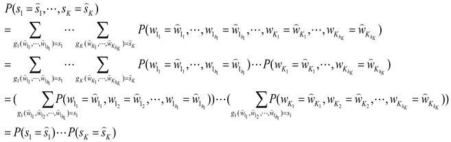
Thus,holds, i.e., are statistically independent. □
As shown in Proposition 1, we have that may effectively explain. Its practical meaning is that adjusting the values of components incontrols the output ofwithout affecting the values of other functions in S, which achieves semantic disentanglement for S.
According to Proposition 1, we know that form a K-partition of the set . Therefore, we use the properties of the K-partition to characterize the degree of coupling among and perform semantic disentanglement. The two sets andmay be approximately described by the following Statement 1:
Statement
1. If for, the values inare far from zero, and conversely, for, the values inare nearly equal to zero, then the degree of coupling amongis low.
Next, to eliminate the influence of sign and magnitude, we define the relative change rate:.
The larger the expectation of, the stronger the explanatory power ofon; conversely, the weaker the explanatory power.
For a K-partition, we propose a disentanglement metric based on the relative change rate, denoted by Formula (6):
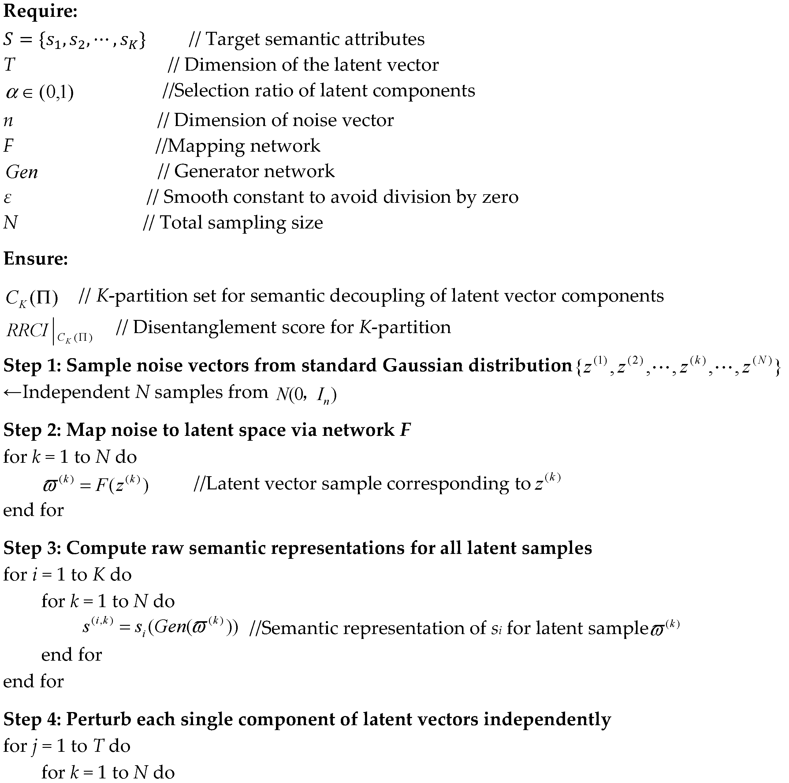
To find the optimal partition and thus achieve semantic disentanglement of S, We propose a latent disentanglement pipeline based on relative change rate, detailed as follows.
Step 1: Set initial conditions. Define the set of semantics ; the latent feature vector ; the latent vector partition ratio; the dimension n of the noise vector; the mapping network F; the generator network G; the smoothing constant; and the sample size N.
Step 2: Sample noise vectors. Independently sample N times from the -dimensional standard Gaussian distribution to obtain the noise vector samples.
Step 3: Compute latent vectors and semantic representations. Using the mapping network F, compute the latent vector samplescorresponding to the noise vector samples, where. Then compute the semantic representations corresponding to each latent vector as,for any.
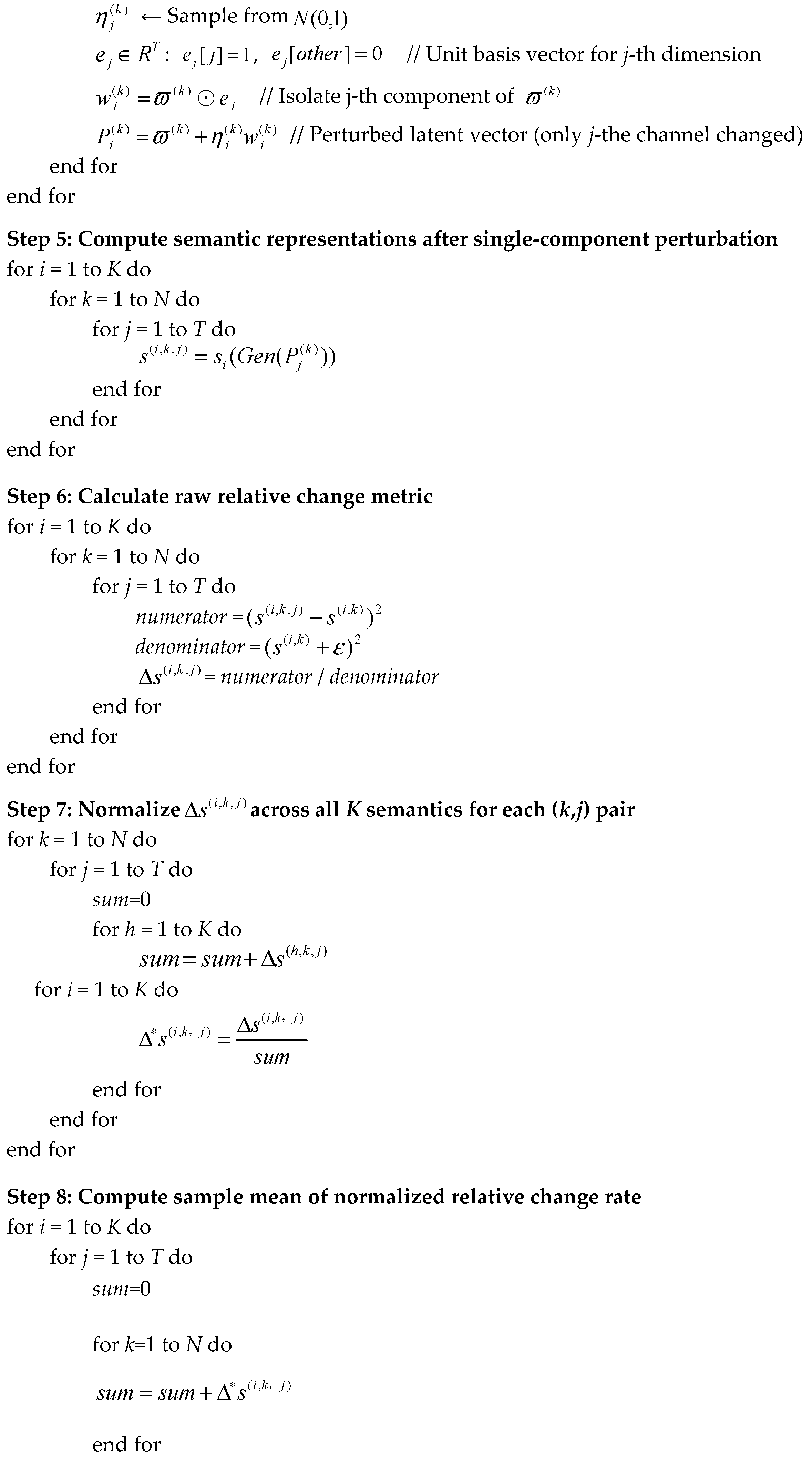
Step 4: Perturb each component of the latent vector samples. For each component of the latent vector samples, perform random perturbation. The perturbed samples for component are denoted as:
where, andis a T-dimensional vector with the j-th component equal to the j-th component of and all other components equal to 0.
Step 5: Compute perturbed semantic representations. Compute the semantic representations corresponding to the perturbed latent vectors:
Step 6: Compute the relative change rate.
Step 7: Normalize the relative change rate.
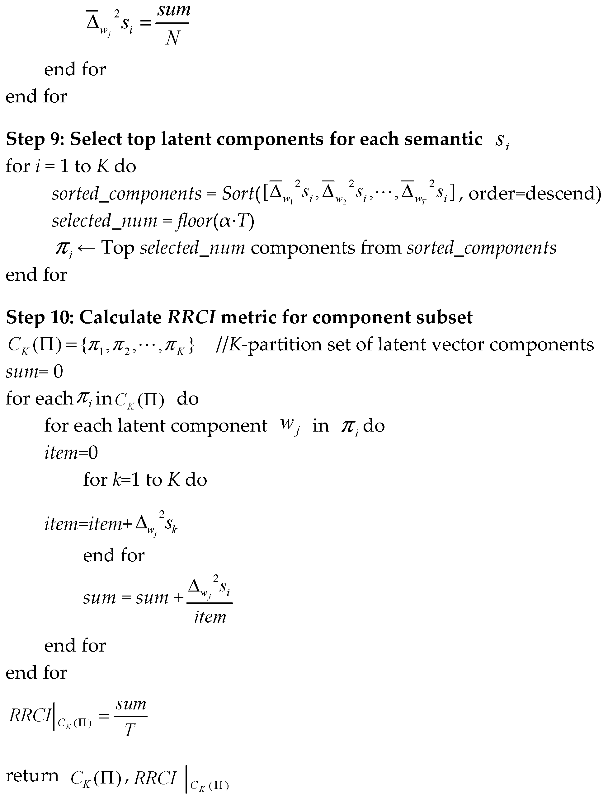
Step 8: Compute the sample mean of the relative change rate.
Step 9: Select explanatory latent vector components for each semantic. For each semantic, sort the sample mean valuesin descending order, and select the topcomponents to form the set.
Step 10: Compute the RRCI metric.
The above disentanglement algorithm based on the relative change rate achieves effective disentanglement of shape and color features in the latent space, addressing the insufficient diversity problem of medical images generated by conventional Gans. In this work, we select the circularity attribute (for foreground shape semantics) and the brightness attribute (for color semantics) as disentanglement targets, whose calculation methods are given by Formula (7) and Formula (8), respectively. Circularity reflects how close the foreground is to a perfect circle, while brightness measures the signal intensity of the foreground region.
whererepresents the enclosed area, andcorresponds to the closed perimeter of the maximum-area external contour derived from input image I. We acquire this contour via Gaussian blurring and subsequent Otsu threshold segmentation operations.is the binary foreground mask generated by the identical preprocessing pipeline; counts all pixels within the mask, andrefers to the normalized intensity of pixel at spatial coordinate.
Algorithm 1 illustrates the complete pipeline of our relative change rate-based latent disentanglement procedure.
| Algorithm 1 Relative Change Rate Based Semantic Disentanglement8 |
|
In the disentanglement experiments, we concatenate the 50-dimensional shape latent vector ϖcolour and the 64-dimensional color latent vector ϖcolour to form a 114-dimensional latent vector. The SCGAN (detailed in Section 3.2.) is adopted as the generator network, with a sample size of 1024. The top 10 components, ranked by the sample mean of the relative change rate, are selected as the disentangled latent vector components for circularity and brightness.
Figure 3 and Figure 4 plot the relative change rates of each component in the 114-dimensional latent feature vector with respect to circularity and brightness, constructing semantic index distribution maps to verify the disentanglement effect of circularity and brightness semantics in the latent feature space. The experimental results show that components with high impact on circularity semantics are concentrated in the first 50 dimensions, which dominate significant variations in the regularity of brain shape. In contrast, components with high impact on brightness semantics are distributed in the subsequent 64 dimensions. This distribution pattern demonstrates the effectiveness of decomposing the latent vector into shape and color vectors: the model successfully disentangles the shape semantics from color semantics in the latent space, and editing of both semantic attributes can be achieved by selecting the top 10 high-impact components for each. Furthermore, the RRCI for circularity and brightness semantics are calculated to be 0.7564.
Figure 5 and Figure 6 visualize the disentanglement effect of brain region circularity and brightness semantics in the latent feature space, achieved by independently editing the selected top 10 core latent components for circularity and brightness. In the circularity editing experiment, modifying the top 10 circularity-specific components increased the brain region circularity from 0.5815 to 0.7196, corresponding to a relative change rate of 23.75%, indicating a significant variation in the shape regularity of the brain region. Meanwhile, brightness only fluctuated slightly from 0.3882 to 0.3688, with a change rate of -4.99%, showing negligible variation. In the brightness editing experiment, modifying the top 10 brightness-specific components caused the brain region brightness to drop drastically from 0.6729 to 0.3453, with a relative change rate of -48.68%, reflecting a substantial reduction in signal intensity. In contrast, the brain region circularity only slightly changed from 0.8182 to 0.7859, with a change rate of -3.95%.These results directly demonstrate that the control of the two semantic attributes—brain region circularity and brightness—is relatively independent.
3.3. The Framework of SCGAN-MultiJNet
SCGAN-MultiJNet mainly consists of two components: SCGAN and MultiJNet. We input noise vectors that control shape and color features, and use SCGAN to generate low-resolution Flair brain tumor images. Then, MultiJNet is employed to synthesize high-resolution Flair images, along with the corresponding multi-modal images (T1, T1ce, T2) and the whole tumor mask. The overall framework of SCGAN-MultiJNet is illustrated in Figure 7.
3.3.1. SCGAN
The proposed SCGAN consists of a generator and a discriminator. By inputting 50-dimensional shape and color noise vectors, SCGAN can generate low-resolution 1×64×64 single-modal Flair brain tumor medical images, whose output serves as the input for the subsequent MultiJNet stage.
The generator of SCGAN is mainly composed of fully connected layers and convolutional layers, with its detailed architecture illustrated in Figure 8. First, the fully connected layers generate color and shape latent features of medical brain tumor Flair images from the input noise vectors.Then, convolutional layers are used to further extract shape features from the images. Next, the color latent features are transformed into convolution kernels and biases, which are then incorporated into the shape feature maps via convolution operations. To avoid drawbacks such as detail blurring and checkerboard artifacts commonly seen in traditional up-sampling techniques (e.g., interpolation and transposed convolution), our method adopts a principle of invariant feature map scale, where the spatial resolution of feature maps is consistently maintained at 64×64 across all stages. To improve the convergence speed and training stability of the model, batch normalization layers and pixel normalization layers are applied after each linear layer and convolutional layer, respectively. During training, the loss function of the generator is composed of structural similarity loss (SSIMLoss), smoothness loss (SLoss), and binary cross-entropy loss (BCELoss), as defined in Formula. SSIMLoss and BCELoss encourage the generated images to more closely approximate the ground truth. The SLoss penalizes the absolute differences between adjacent pixels, forcing the pixel values of the generated images to be smoother in both horizontal and vertical directions, thereby reducing high-frequency noise. Meanwhile, a weight parameteris introduced to control the strength of the SLoss.
where,
(1) denotes the synthetic Flair brain tumor image generated by the generator, an is real Flair image.
(2) Letbe the convolution operation implemented with a Gaussian convolution kernel.denotes element-wise multiplication.-denotes element-wise division. denote fixed constants.denotes the mathematical expectation calculated.
(3) Letbe the weight..
(4) Letrepresent the output of discriminator network , anddenote the all-one target label ..
Figure 8.
Generator Architecture of SCGAN.
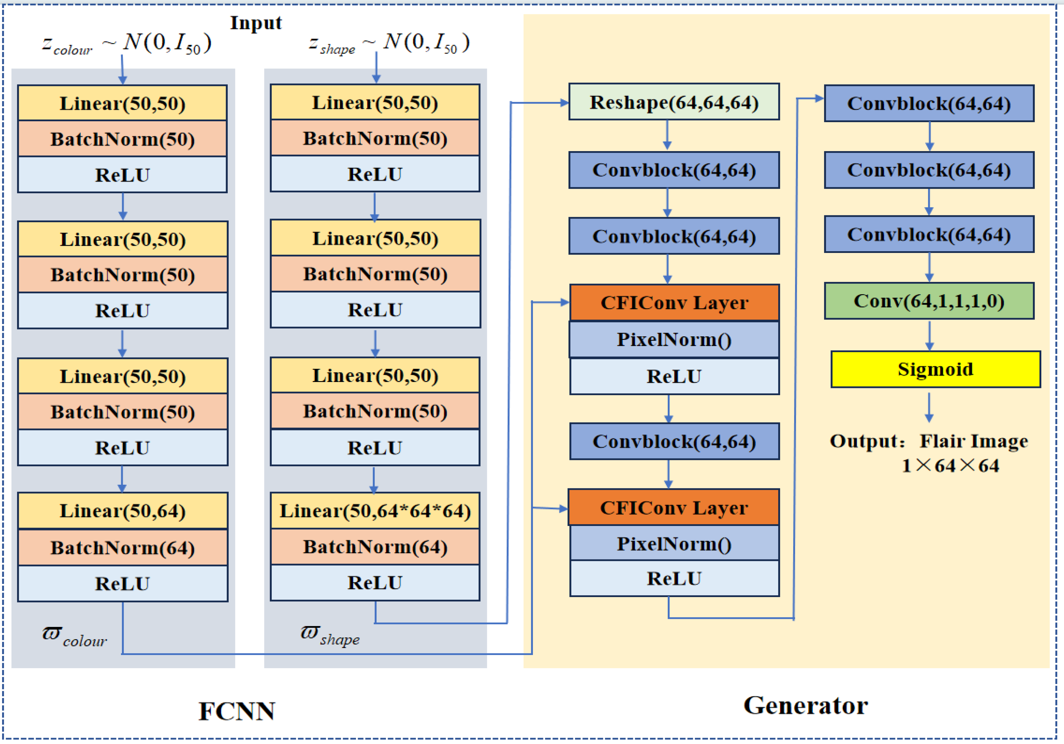
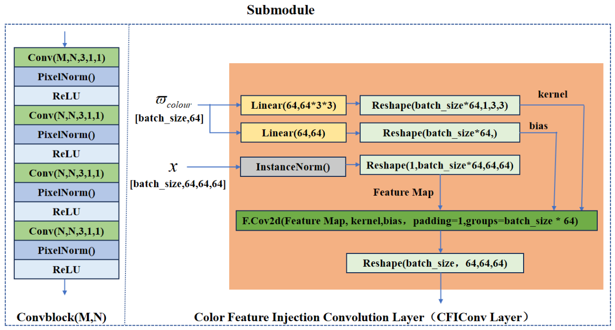
In SCGAN, we construct CFIConvLayer, a color-conditioned dynamic convolution layer for disentangled image generation. It has three core functions:
First, it achieves grayscale modulation via dynamic convolution kernel generation. Instead of using fixed convolution parameters, all convolution kernels and biases are dynamically mapped from the color latent vector. Each sample and each feature channel is equipped with an independent 3×3 convolution kernel, allowing the model to flexibly adjust image grayscale intensity according to different pathological states and imaging modalities.
Second, it enables the disentanglement of shape and color. The spatial structural features of the brain outline and position are fed solely by the shape branch; the CFIConvLayer only adjusts the amplitude of feature activations without modifying spatial structural information.
Third, by invoking this module twice at different network levels in the generator, it sequentially performs coarse-grained modality information injection and fine-grained texture grayscale optimization, achieving multi-scale refined color injection.
The CFIConvLayer is defined by Formula:
whereis the spatial shape feature map; is the color latent vector; denotes instance normalization;andare fully-connected mapping layers that generate the dynamic convolution kernels and biases, respectively; theenables per-sample and per-channel independent convolution, completing the conditional modulation of spatial features by color features.
Drawing inspiration from the discriminator design of StyleGAN, the discriminator of SCGAN adopts an architecture of progressive down-sampling plus feature extraction to distinguish the authenticity of input images. The SCGAN discriminator extracts multi-scale features of images through layer-wise nearest-neighbor interpolation down-sampling. Using nearest-neighbor down-sampling reduces information loss during the down-sampling process while maintaining computational efficiency. Meanwhile, the SCGAN discriminator integrates modules from StyleGAN, such as PixelNorm and MiniBatchStdDev [36]. The MiniBatchStdDev computes the standard deviation of features within each batch, enhancing the discriminator ability to detect mode collapse in generated samples and further improving the diversity of generated outputs. The detailed architecture of the SCGAN discriminator is illustrated in Figure 9. The loss function of the discriminator is composed of BCELoss between the generated images and real images, as defined in Formula:
Where;;;
3.3.2. MultiJNet
The generator of SCGAN takes Gaussian noise as its initial input. Since the noise itself lacks structured image information, the brain tumor images it generates suffer from problems such as low resolution, significant inherent noise interference, and blurred lesion details and edge contours, making it difficult to recover the fine structural features of real medical images. To improve the quality and resolution of Flair images generated by SCGAN, we introduce JNet.
U-Net features a U-shaped architecture with symmetric contracting and expanding paths. A key characteristic of U-Net is its use of skip connections to combine features from the encoder and decoder, which helps preserve more spatial information [37]. Inspired by the encoder-decoder structure design of U-Net, JNet is a convolutional neural network based on residual blocks, encoders, and decoders. Unlike U-Net, which uses max pooling for down-sampling after convolution, JNet employs convolution with a stride of 2 for down-sampling, which helps retain local image information. The decoder recovers spatial resolution through up-sampling, and multi-scale feature fusion is achieved via skip connections. Additionally, residual blocks are used throughout the entire network to avoid gradient vanishing and improve feature reuse. The detailed architecture of JNet is illustrated in Figure 10. The loss function of JNet adopts mean squared error (MSE) loss. During training, JNet takes low-quality Flair images—corrupted by down-sampling, multiple Gaussian noises, and median blur—as input, with high-resolution Flair images serving as the ground truth. After optimization, JNet improves the resolution and image quality of Flair images generated by SCGAN.
Considering the multi-modal nature of brain tumor medical image datasets, we adopt multiple independent JNet models to perform cross-modal translation tasks from the Flair modality to three other modalities (T1, T1ce, and T2), as well as the automatic annotation task of brain tumor regions. Each JNet model focuses on a single sub-task, which not only facilitates efficient training and performance optimization but also better meets the core requirement of multi-objective multi-task learning in multi-modal datasets generation scenarios. Finally, the MultiJNet ensemble architecture, constructed from five JNet units, enables the efficient generation of multi-modal brain tumor medical images.
3.3.3. Image Synthesis Based on SCGAN-MultiJNet Algorithm
Aiming at the difficulty in annotating multi-modal brain tumor MRI data, the proposed SCGAN-MultiJNet is adopted to synthesize high-quality multi-modal MRI images, which can provide reliable data augmentation for downstream brain tumor analysis tasks. The specific implementation pipeline of the image synthesis is presented in Algorithm 2.
| Algorithm 2 SCGAN-MultiJNet Multi-modal MRI Brain Tumor Image Synthesis |
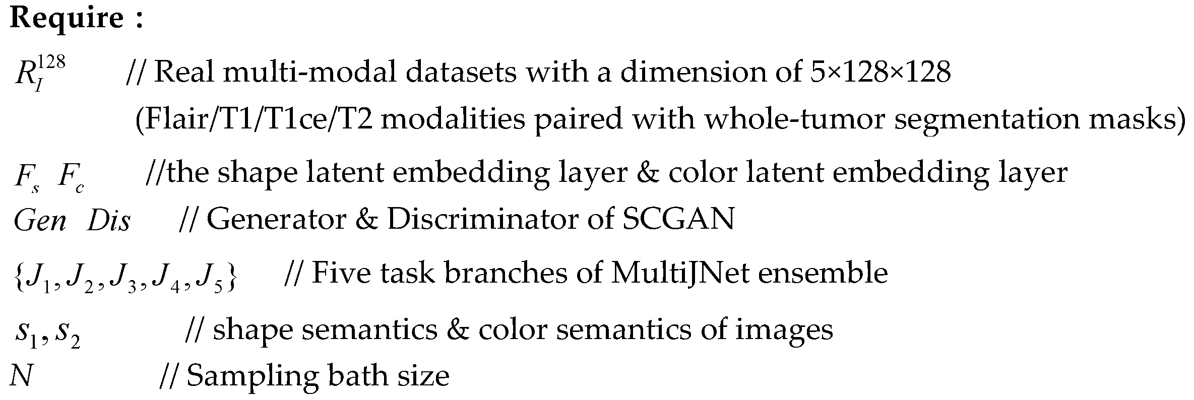 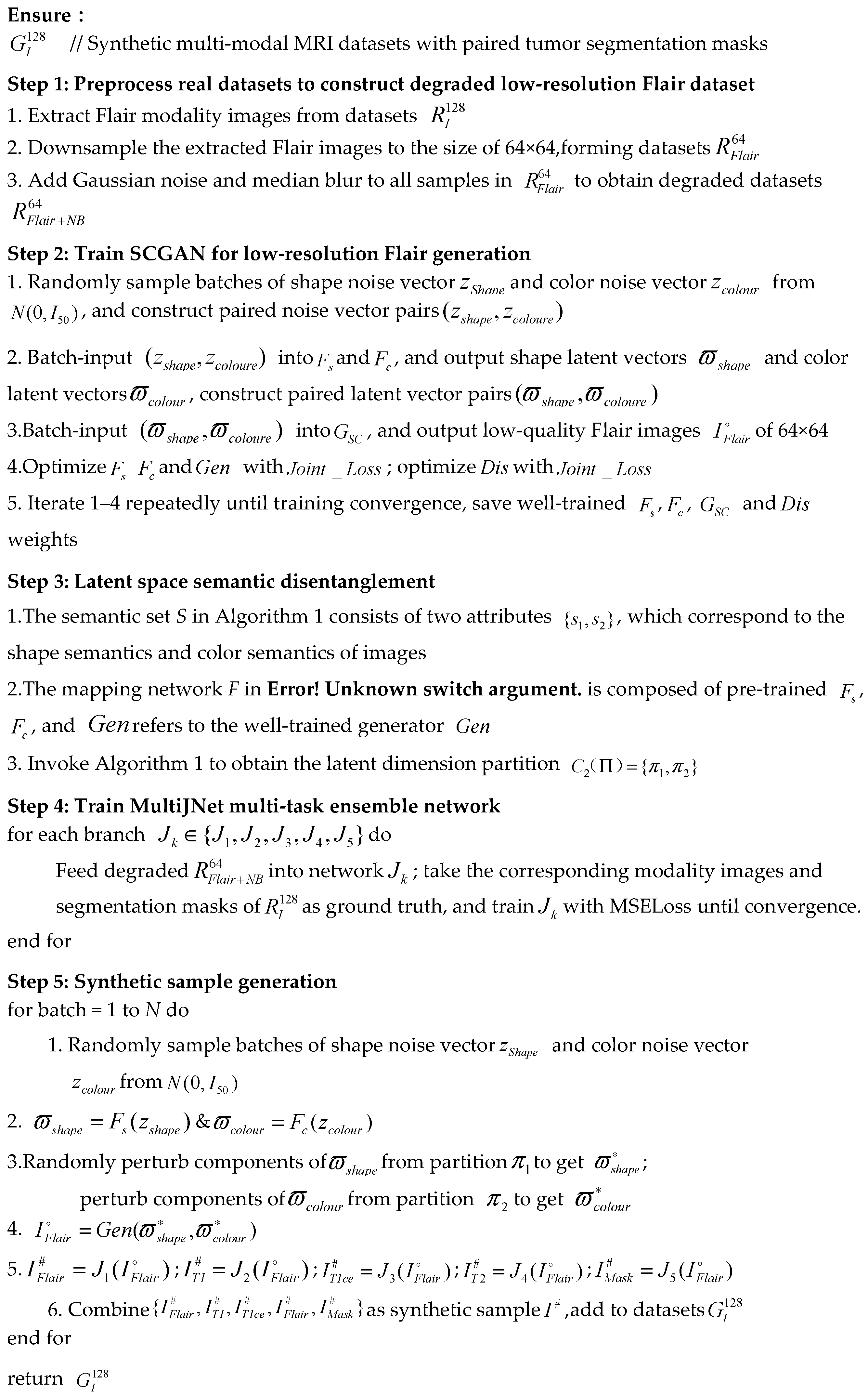
|
4. Image Generation Experiment
4.1. Datasets Introduction
In this work, we use the BraTS2020 datasets to validate the performance of SCGAN-MultiJNet [2,3,4]. The BraTS datasets is a key resource from the MICCAI Brain Tumor Segmentation Challenge. These data were acquired from multiple scanners at 19 different institutions using varying clinical protocols. To ensure consistency, all images were manually segmented by one to four reviewers following a unified annotation protocol. All multi-modal images in BraTS2020 are provided in NIfTI format, with a total size of 39.8 GB. The BraTS2020 datasets includes 369 cases in the training datasets and 125 cases in the validation datasets. Each case covers four modalities: Flair, T1, T2, and T1ce. Additionally, the datasets defines three segmentation regions: enhancing tumor (ET - label 4), peritumoral edema (ED-label 2), and necrotic/non-enhancing tumor core (TC-label 1). Both the images of each modality and their corresponding annotations are presented as 3D data with a spatial resolution of 155×240×240.
4.2. Data Preprocessing
In this study, we selected samples numbered from 0 to 300 from the BraTS2020 datasets as the research objects. For annotation processing, we unified the regions labeled 1, 2, and 4 as 1 (representing the foreground region of interest), while setting all other regions to 0, thereby creating WT images to facilitate subsequent image processing and analysis. The data preprocessing steps are as follows:
Step 1: Slice the four modality images and annotation images of each case along the third axis, selecting one slice every five slices to ensure data representativeness. Meanwhile, samples containing no foreground information are removed.
Step 2: Apply percentile-based z-score normalization to the four modality images, removing the top and bottom 0.01% outliers in pixel values.
Step 3: To save computational resources, down-sample the image slices from 240×240 to 128×128 using area interpolation, preserving image details while forming 3960 samples.
Step 4: Use the Isolation Forest anomaly detection model to clean 10% of the 3960 samples as anomalies, resulting in a datasets of 3564 samples with a size of 5×128×128.
The preprocessed datasets is used as the real image input for SCGAN-MultiJNet. To distinguish it from the generated data described later, this real datasets is denoted as R. Meanwhile, R also serves as part of the training data for the segmentation network described in subsequent sections. To prevent information leakage, we selected samples numbered from 301 to 369 from the BraTS2020 datasets and performed the same preprocessing operations to form a test datasets of 826 samples with a size of 5×128×128, denoted as Rtest, which is used to validate the segmentation performance of the segmentation network.
Since SCGAN generates low-resolution Flair images, we further compress Flair images of R from 128×128 to 64×64, forming a datasets denoted as R64. To boost the robustness of MultiJNet, we introduce Gaussian noise (50 iterations, mean = 0, standard deviation = 0.05) and median blur to datasets R64 to construct a degraded datasets R64+NB. This operation renders the synthesized images more consistent with low-quality Flair outputs generated by SCGAN, thereby further strengthening the generalization capacity of MultiJNet. Figure 11 shows a comparison between the original image and the blurred image.
4.3. Environmental Configuration and Hyperparameter Settings
All experiments were conducted on a computer equipped with an NVIDIA GeForce RTX 3060 GPU and 16 GB RAM. The SCGAN-MultiJNet model was trained based on PyTorch 2.2.2 and its associated libraries. Table 1 presents the detailed hyperparameter settings adopted in this study. During training, the AdamW and Adam optimizers were utilized to update parameters of SCGAN and JNet respectively.
4.4. SCGAN-MultiJNet Image Generation Visualization
Figure 12 displays brain Flair images generated by SCGAN at different training epochs. Each row corresponds to a specific epoch, visually illustrating the dynamic evolution of image quality and fine details. At epoch 20, the model initially captures basic shape features. However, the generated images suffer from poor quality, severe noise interference and blurred details. At epoch 45, the model further learns color distribution characteristics. The image quality and detail clarity are improved, though slight blurriness and noise still remain. At epoch 75, abundant texture details are acquired. Textural patterns become distinct, noise is largely suppressed, and visual consistency with real Flair images is significantly enhanced. As training proceeds, the quality of images generated by SCGAN gradually improves. The model sequentially learns feature representations of shape contour, color distribution and texture details. This learning pattern conforms to the architectural design of SCGAN.
The single-modal Flair images generated by SCGAN only have a resolution of 64×64 with inferior image quality. Accordingly, the MultiJNet model is adopted to improve image resolution and quality, and accomplish cross-modal conversion and automatic brain tumor segmentation simultaneously. A total of 3564 noise vectors containing shape and color features are fed into fully connected layers to obtain corresponding shape and color latent vectors. Random perturbations are imposed on the top 10 core latent components of circularity and brightness to expand the feature distribution range. The optimized vectors are then imported into the overall SCGAN-MultiJNet framework to generate 3564 multi-modal brain tumor MRI images, forming a synthetic datasets denoted as G (Details are given in Algorithm 2). Figure 13 presents representative generated samples. The four modalities of each image maintain high consistency in spatial structure. Meanwhile, the generated tumor labels exhibit diverse sizes and morphological patterns. Considering the difficulties and high costs of acquiring real clinical medical images, the synthetic datasets G can be applied to augment the real training datasets R, so as to boost the performance of the segmentation network.
4.5. Ablation Experiment
As the core feature fusion module in SCGAN, the CFIConv Layer performs dimension transformation and mapping on color latent features to generate convolution kernels and biases matching the size of feature maps. It deeply integrates color and shape features via convolution operations, realizing joint optimization of color and spatial characteristics.
JNet is a residual-based encoder-decoder network with skip connections and multi-scale feature fusion branches. It takes low-quality, low-resolution degraded Flair images as input, restores fine lesion textures and edge details through upsampling and residual learning, and completes cross-modal translation from Flair to T1, T1ce, T2 as well as tumor mask prediction when assembled into MultiJNet ensemble.
SSIMLoss and SLoss jointly guide and constrain the image generation process. SSIMLoss evaluates structural similarity between generated and real images by measuring discrepancies in luminance, contrast and structure. SLoss restricts pixel smoothness and suppresses artifacts such as sawtooth edges and noise points.
In this paper,We adopt five quantitative metrics to comprehensively evaluate image generation quality. Fréchet Inception Distance (FID) evaluates the distribution similarity between synthetic and real images via features from the Inception network; lower FID means more consistent feature distribution and better generation quality. As a kernel-based metric, Maximum Mean Discrepancy (MMD) measures distribution divergence in reproducing kernel Hilbert space, with smaller values indicating higher distribution similarity. Inception Score (IS) evaluates intra-class recognizability and inter-sample diversity of generated images, where a higher IS denotes recognizable image with abundant morphological and grayscale variations. Peak Signal-to-Noise Ratio (PSNR) complements SSIM for pixel-level reconstruction evaluation: SSIM measures global similarity in structure, luminance and contrast, while PSNR directly calculates pixel grayscale distortion between synthetic and real images, and higher PSNR corresponds to less noise and smaller.
To quantitatively verify the independent contribution and synergistic interaction of the four core components including CFIConvLayer, JNet, SSIMLoss and SLoss in the proposed SCGAN-MultiJNet framework, two sets of ablation experiments are carried out, covering 64×64 single-modal Flair low-resolution generation and 128×128 complete multi-modal generation tasks. Five complementary quantitative metrics (FID, MMD, IS, PSNR and SSIM) are adopted to evaluate the generation performance from three dimensions: high-dimensional feature distribution matching, sample diversity and pixel-level anatomical structural fidelity, and all ablation results are summarized in Table 2.
According to the ablation results listed in Table 2Table 1, Group A acts as the baseline only equipped with the original GAN backbone and BCELoss. After introducing CFIConvLayer (Group A→B), the FID drops from 50.5578 to 44.9116 and MMD decreases from 0.1798, accompanied by mild improvements of PSNR and SSIM. This indicates that CFIConvLayer can generate independent convolution kernels according to color latent vectors to realize decoupled modulation of image contour and grayscale features, effectively narrowing the feature distribution gap between synthetic and real images. Nevertheless, the IS only rises slightly, revealing that the single feature fusion module cannot significantly enrich the morphological diversity of images. On the basis of Group B, the introduction of SSIMLoss (Group B→C) brings a sharp increase of IS from 1.6832 to 2.0836, and MMD reaches the minimum value of this subgroup. The SSIMLoss constrains the consistency of luminance and contrast between generated and real images. Although FID has a slight rebound due to the trade-off between structural restriction and latent distribution smoothness, the pixel structural metric SSIM remains stable at a high level. Further adding SLoss (Group C→D) makes FID and MMD drop to the optimal level, yet IS decreases obviously. The smooth regularization suppresses high-frequency noise and jagged artifacts, but it compresses the latent variation range and leads to homogenized synthetic samples.
For the 128×128 full SCGAN-MultiJNet ablation series, Group A0 serves as the complete baseline only using the backbone network and bilinear upsampling without JNet, CFIConvLayer and auxiliary loss terms. After embedding the JNet multi-scale reconstruction module (Group A0→A1), FID falls sharply from 64.5534 to 12.4144 and MMD reduces from 0.5201. This proves that the JNet with skip connections is the core module for eliminating feature distribution offset. Simply stacking CFIConvLayer upon JNet (Group A1→B0) leads to severe deterioration of distribution metrics, with FID jumping to 48.8585. It demonstrates that CFICConvLayer cannot function independently; the dynamic grayscale modulation operation will break the global feature distribution learned by JNet in the absence of structural loss constraints, and only minor promotions on pixel metrics and IS can be observed.
Adding SSIMLoss to Group B0 constructs Group C0, which achieves balanced optimal performance. FID falls back to 29.0166, MMD hits the lowest value among all 128×128 ablation groups, and both IS and SSIM are further improved. SSIMLoss effectively remedies the negative influence of CFIConvLayer on feature distribution. When SLoss is further introduced on the basis of Group C0 to form D0, FID surges to 59.2537 and MMD rises simultaneously. Although IS reaches the highest value across all groups, SLoss excessively blurs subtle pathological textures and weakens the distinguishability of latent semantic components, resulting in obvious feature distribution drift.
Overall, JNet is the indispensable core reconstruction module to reduce distribution discrepancy between synthetic and real samples. CFIConvLayer can effectively decouple shape and color latent features only under the constraint of SSIMLoss. SSIMLoss acts as the balanced regularization term to coordinate the performance of multiple modules. SLoss brings obvious negative trade-offs (Note: The SLoss module is still introduced in this paper to improve the robustness and generalization of downstream segmentation networks when the model uses synthetic datasets G for data augmentation). The combination of Backbone +JNet+CFIConvLayer+BCE+SSIMLoss achieves comprehensive superiority on multiple evaluation indicators, and the effectiveness of each proposed component is fully verified through quantitative ablation experiments.
5. Data Augmentation Experiment Using the Synthetic Multimodal Brain Tumor Dataset G
In this section, we conduct data augmentation experiments using the generative multi-modal brain tumor datasets G. Owing to its proven strong segmentation performance, U-Net [37] is adopted as the segmentation network to evaluate the augmentation effectiveness of datasets G.
The four modalities—Flair, T1, T1ce, and T2—are fed into U-Net as four input channels. To mitigate overfitting, dropout layers with a rate of 0.1 are appended after each convolutional layer in the network. The Adam optimizer is employed for training the U-Net segmentation model. The training hyperparameters are set as follows: the maximum number of epochs is 180, the batch size is 32, and the initial learning rate is set to 1e-05. BCELoss is used as the loss function.
5.1. Evaluation Metrics for Segmented Networks
To comprehensively evaluate the performance changes of the segmentation network before and after data augmentation, five metrics are selected for quantitative analysis: Accuracy, Dice coefficient, Precision, Recall, and Intersection over Union (IoU). The definitions and interpretations of these metrics are given in Formula to Formula (16).
This metric measures the overall correctness of the model predictions across all samples.
This metric quantifies the similarity between predicted segmentation results and ground truth labels, serving as a core evaluation metric in medical image segmentation tasks.
This metric reflects the proportion of true positive samples among all predicted positive results, measuring the precision of the predictions.
This metric represents the proportion of true positive samples correctly identified by the model, reflecting the model sensitivity to positive samples.
This metric measures the ratio of the intersection area between predicted and ground truth positive regions to their union area, serving as a key indicator for evaluating the matching degree of target regions in segmentation tasks.
5.2. Design of the Training Datasets for the Segmented Network and Experimental Results
The training datasets of the segmentation network U-Net is constructed by combining the real datasets R and the generative datasets G in different ways (Note: R and G are defined in Sections 4., respectively). Both R and G contain 3564 samples. Two main strategies are adopted for training datasets design.
Case 1: Proportional Mixing
The total number of training samples is fixed at 3564. Samples are randomly drawn from R and G to form training datasets with different mixing ratios, specifically R:G = 20:80,40:60, 60:40, and 80:20. The notation R:G = 20:80 indicates that the proportion of samples from R and G in the training datasets is 20% and 80%, respectively. Notably, R:G = 100:0 and R:G = 0:100 represent training datasets composed entirely of R or G, respectively.
Case 2: Incremental Augmentation
The total number of training samples is gradually increased by combining all samples from R with varying proportions of G. The fractions of G randomly selected are 0, 0.2, 0.4, 0.6, 0.8, and 1, where 0 and 1 correspond to selecting none or all samples from G, respectively. The notation R+0.2*G indicates that the training datasets consists of all samples from R plus 20% of samples from G.The symbol * represents the multiplication operation.
To verify whether the generated data can achieve comparable training performance to real data, the real datasets Rtest is uniformly used as the test set for the segmentation network across all above training datasets configurations.
5.2.1. Experimental results for Case 1
Figure 14 illustrates the dynamic trends of various performance metrics of the U-Net segmentation network on the training datasets under different mixing ratios of the real datasets R and the synthetic datasets G. The experimental results show that, even as the proportion of synthetic data in the training set continuously increases, the model training state remains stable, and the trends of all metrics exhibit high consistency.
Table , together with the line charts and radar charts in Figure 15, illustrates the trends of evaluation metrics on the test datasets as the proportion of real data decreases. When the model is trained solely on real data (i.e., R:G=100:0), core metrics including Accuracy, Dice coefficient, and IoU all remain at high levels, indicating that pure real data provides a high-quality training foundation for the segmentation network and yields stable target recognition and segmentation performance. When a small proportion of synthetic data is introduced into the training datasets (i.e., R:G=80:20), Precision increases from 0.9111 to 0.9167, while Accuracy, IoU, Dice coefficient, and Recall exhibit minor fluctuations. As the proportion of synthetic data becomes excessively high (e.g., R:G=40:60 and R:G=20:80), Accuracy, IoU, Dice coefficient, and Recall begin to decline further, as the distribution shift of synthetic data significantly impairs the segmentation completeness of the model. When trained solely on synthetic data (i.e., R:G=0:100), Accuracy, IoU, Dice coefficient, and Recall all reach their lowest values in the entire group, while only Precision achieves the highest value. This indicates that the distribution shift between synthetic and real data prevents the model trained on synthetic data from fully generalizing to the real test datasets. From the line charts, it is observed that the two core metrics in medical image segmentation—Dice coefficient and IoU—exhibit highly consistent trends: both decrease as the proportion of synthetic data increases, showing equal sensitivity to changes in data distribution.

Table 3.
Metrics of Segmentation Network U-Net on Rtest in Case1.
| R: G | Accuracy | Dice | Precision | Recall | IoU |
| 100: 0 | 0.9857 | 0.8904 | 0.9111 | 0.8710 | 0.8030 |
| 80:20 | 0.9855 | 0.8892 | 0.9167 | 0.8638 | 0.8008 |
| 60: 40 | 0.9847 | 0.8804 | 0.9253 | 0.8404 | 0.7868 |
| 40:60 | 0.9847 | 0.8801 | 0.9208 | 0.8435 | 0.7862 |
| 20:80 | 0.9838 | 0.8750 | 0.8943 | 0.8572 | 0.7789 |
| 0:100 | 0.9767 | 0.7987 | 0.9378 | 0.6977 | 0.6664 |
5.2.2. Experimental Results for Case 2
Figure 16. Metrics of the U-Net on the Training Datasets in Case2. presents the variation of segmentation metrics when gradually adding synthetic datasets G into the training set. The consistent trends across all sub-graphs demonstrate that the quantity of incorporated synthetic samples exerts limited influence on U-Net training performance. The segmentation network possesses compatibility with synthetic data.
Figure 16.
Metrics of the U-Net on the Training Datasets in Case2.
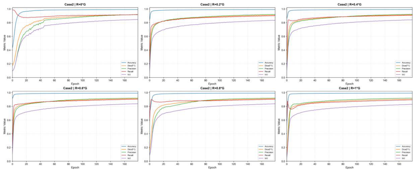
Table 4 and Figure 17 present the performance of the U-Net segmentation network on the test set when trained with real data augmented by different proportions of synthetic data. According to the results in Table 4, when the model is trained solely on real data, all metrics except Recall are at their lowest levels. As the amount of synthetic data increases, the metrics fluctuate: when the training datasets is R+0.2*G, R+0.4*G, or R+0.6*G, Accuracy, IoU, Dice coefficient, and Precision improve, while Recall decreases. When the training datasets is R+0.8*G, the model achieves the optimal values for Accuracy, IoU, and Dice coefficient, showing the best overall performance. However, when all synthetic data is added, Accuracy, Dice coefficient, and IoU decline again. The line chart in Figure 14 shows that Accuracy remains generally stable, Precision exhibits an upward trend with increasing synthetic data, while Dice coefficient and IoU rise significantly when the training datasets is R+0.8*G. The radar chart reveals that the polygon area corresponding to R+0.8*G is the largest, indicating the best comprehensive performance at this mixing ratio. Overall, in Case 2, adding 80% of the synthetic data to the real datasets is the optimal mixing strategy for the U-Net segmentation model to achieve the best test performance.
5.2.3. Comparison of Segmentation Network Predictions Before and After Augmentation
Figure 18 presents the segmentation results of the U-Net model under two training datasets configurations: without data augmentation (R) and with data augmentation (R+0.8*G). The first row corresponds to compact and simple brain tumor lesions: whether data augmentation is applied or not, the predicted shapes for simple regions are generally consistent with the ground truth labels.
The second row shows complex lesions with irregular shapes: the model trained only on original real data exhibits significant internal missegmentation and large deviations from the ground truth. In contrast, the model trained with synthetic data augmentation shows substantially reduced missegmentation regions and better alignment of contours with the ground truth. The third row displays highly complex multi-branched lesions: the model without augmentation suffers from severe missegmentation (predicting an irrelevant region at the bottom), with notable discrepancies between the main lesion boundary and the ground truth. The augmented model eliminates missegmentations, achieving a significant improvement in shape matching with the ground truth.
In summary, the model trained on real data augmented with an appropriate amount of synthetic data effectively improves segmentation performance: it reduces under- segmentation, eliminates missegmentation, yields predicted shapes closer to the ground truth, enhances boundary accuracy, and significantly boosts the overall performance of the segmentation model.
5.3. Robustness Experiment
To comprehensively evaluate the robustness of the augmented model (R+0.8*G) in real clinical scenarios, this study constructed a robustness test datasets with 8 common types of medical image perturbations: Gaussian noise, Gaussian blur, brightness shift, contrast variation, Gamma correction, bias field artifact, block occlusion, and down-sampling blur. Five levels of perturbation severity, ranging from low to high, were set. Robustness performance was assessed by comparing the percentage drops in five metrics (Accuracy, IoU, Dice, Precision, and Recall) of the augmented model (R+0.8*G) and the baseline model ( R) under these perturbations relative to Rtest.
It can be seen from the subgraph curves corresponding to Gaussian blur, bias field artifact and down-sampling blur in Figure 19 that the curves of the augmented model trained with the (R+0.8*G) scheme always lie below those of the baseline model under all five perturbation severity levels, and the gap between the two curves widens continuously as the perturbation intensity rises. The baseline model is trained merely on high-quality real images from a single source, leading to insufficient diversity of sample features. When images are disturbed by heavy blur and severe intensity offset, the decline curves of the Dice coefficient and Recall increase sharply. In contrast, the proposed SCGAN-MultiJNet generates numerous synthetic images with diverse tumor contours and grayscale distributions via the shape-color disentangled latent space. By mixing synthetic samples into the training set, the segmentation performance degradation caused by severe clinical image distortion can be effectively suppressed.
For brightness shift, Gamma correction and block occlusion, the overall variation trends of the two groups of curves are similar, yet the augmented model achieves smaller declines in core segmentation metrics (Dice and IoU) at all perturbation intensities. The curve pattern of Gaussian noise differs remarkably from other distortion types. At low noise levels (Level 1 and Level 2), the metric decline curves of the two models almost overlap with negligible performance differences. Nevertheless, the curve of the augmented model rises steeply under the maximum Level 5 noise intensity.
An analysis of core evaluation metrics including the Dice decline curve and IoU decline curve in Figure 19 demonstrates that obvious gaps exist in the Dice and Recall curves between the two models across eight perturbation scenarios: Gaussian blur, brightness shift, contrast variation, Gamma correction, bias field artifact, block occlusion and down-sampling blur. The lower decline curves of the augmented model intuitively verify that synthetic data augmentation can effectively alleviate under-segmentation and mis-segmentation under image distortion. Since normal background pixels account for a large proportion in brain MRI images, the fluctuation range of the Accuracy curves is limited; however, the augmented model still suffers less performance loss under all types of disturbances. In terms of Precision, the augmented model achieves superior values under severe bias field artifacts, block occlusion and Gamma distortion.
The curve trends of all perturbation subgraphs collectively lead to the conclusion that expanding the training set with synthetic images generated by SCGAN-MultiJNet can effectively improve the segmentation mode’s adaptability to various clinical MRI imaging defects, and the robustness gain becomes more prominent as image distortion aggravates. Benefiting from the dual-branch latent disentanglement design, the proposed network broadens the feature distribution coverage of training samples and reduces the model’s over-reliance on single high-definition MRI textures, thereby maintaining stable segmentation performance under complex clinical scanning conditions.
5.4. Generalization Experiment
As shown in Table from the augmentation experiments, the real datasets R and the synthetic datasets G exhibit distinct distribution characteristics. Therefore, the training datasets obtained by combining R and G in different proportions are used to construct a dual-source mixed training domain for multi-source domain generalization experiments. We select the BraTS2025-SSA-Data [38] as the out-of-domain test set for evaluation, and no prior information from this test set is introduced during model training. The means and variances of R, G, and BraTS2025-SSA-Data in Table demonstrate the distribution discrepancies among the three datasets.
Table 5.
Statistical Distribution Comparison of R, G and BraTS2025-SSA-Data Datasets.
| Dateset | Mean | Var |
| R | 0.2187 | 0.0694 |
| G | 0.2041 | 0.0558 |
| BraTS2025-SSA-Data | 0.2341 | 0.0788 |
Table 6.
Metrics of Segmentation Network U-Net on BraTS2025-SSA-Data in Case1.
| R: G | Accuracy | Dice | Precision | Recall | IoU |
| 100: 0 | 0.9617 | 0.6802 | 0.5853 | 0.8219 | 0.5186 |
| 80:20 | 0.9665 | 0.6971 | 0.6302 | 0.7983 | 0.5409 |
| 60: 40 | 0.9525 | 0.6238 | 0.5176 | 0.8037 | 0.4592 |
| 40:60 | 0.9531 | 0.6282 | 0.5201 | 0.8063 | 0.4620 |
| 20:80 | 0.9427 | 0.5755 | 0.4613 | 0.7992 | 0.4098 |
| 0:100 | 0.9559 | 0.5851 | 0.5558 | 0.6326 | 0.4168 |
Table and Table 7 present the results of multi-source domain generalization comparison experiments under the two fusion strategies (Case 1 and Case 2) of R and G, quantitatively analyzing the effects of different combinations of real data R and synthetic data G on the cross-domain generalization ability of the model.
According to the proportional mixing results of Case 1 in Table , the model trained with pure real data (R:G=100:0) exhibits certain cross-domain segmentation performance. As the proportion of synthetic data G gradually increases, the comprehensive cross-domain metrics of the model first rise and then decline. Among them, the combination (R:G=80:20) achieves optimal values in Accuracy, Dice coefficient, Precision, and IoU. The introduction of a small amount of synthetic data can enrich the training representations by leveraging the distribution discrepancy between the two domains, effectively mitigating single-domain over-fitting and enhancing out-of-domain generalization ability. When the proportion of synthetic data continues to increase from 60:40 to 0:100, core segmentation metrics such as Dice coefficient and IoU show a downward trend. The model trained by pure synthetic data(0:100) exhibits significantly degraded generalization performance, indicating that over-reliance on synthetic domain data introduces distribution shifts and weakens the model adaptability to real out-of-domain data.
The results of Case 2 (incremental augmentation) in Table 7 show that adding a small amount of synthetic data to all real data, i.e., the combination R+0.2*G, yields the best cross-domain generalization performance. All segmentation metrics are significantly superior to those of the baseline model, demonstrating that moderately introducing synthetic samples with distribution discrepancy can construct a stable dual-source mixed training domain and improve the model adaptive ability to unknown out-of-domain data. As the amount of added synthetic data continues to increase, model generalization performance gradually declines, limiting its cross-domain inference capability.
Combining the results of Table and Table 7, real data and synthetic data exhibit distribution differences. Reasonably combining them to construct a dual-source training domain can significantly improve the cross-domain generalization performance of the segmentation model. Using a small amount of synthetic data to assist training is an effective strategy to enhance cross-domain generalization ability.
6. Conclusions
This paper addresses the problem of data scarcity in multi-modal MRI brain tumor segmentation by proposing a data synthesis algorithm based on SCGAN-MultiJNet. First, SCGAN constructs a data generation framework to simulate the feature distribution of real multi-modal brain tumor images and synthesize low-resolution data. Then, the multi-scale feature extraction and fusion mechanism of MultiJNet is leveraged to improve the quality and semantic consistency of the generated data. Meanwhile, the SCGAN generative model adopts a shape-color dual-branch semantic disentanglement paradigm for the latent space, and establishes a disentanglement quantitative evaluation method centered on relative change rate, achieving effective disentanglement of the two semantic dimensions.
In the experiments, training datasets constructed by combining real and synthetic data in different ways are used to train the U-Net model. Compared with the baseline model trained solely on real data, the proposed method effectively reduces under-segmentation in complex lesion regions and missegmentation in multi-branched lesions. Key evaluation metrics including Dice coefficient and IoU are significantly improved. The results verify the effectiveness of the SCGAN-MultiJNet-based data augmentation algorithm in enhancing model robustness and cross-domain generalization ability.
The proposed SCGAN-MultiJNet data synthesis algorithm provides a new technical solution for multi-modal brain tumor segmentation, effectively breaking through the bottleneck of data scarcity. It further improves the segmentation performance of the model, offering more reliable technical support for clinical applications.
Author Contributions
Conceptualization,X.F. and X.W. ; methodology,X.F.; software, X.F.; validation, X.F.; data curation, M.J.C. Samonte; writing—original draft preparation, X.F.; writing—review and editing, X.F. and X.W.; visualization, X.F.; supervision,M.J.C.Samonte and X.W.; project administration, X.F.; funding acquisition,X.W. All authors have read and agreed to the published version of the manuscript.
Funding
This work was supported in part by the National Natural Science Foundation of China under Grant No.62376212.
Institutional Review Board Statement
Not applicable.
Informed Consent Statement
Not applicable.
Data Availability Statement
The raw data supporting the conclusions of this article will be made available by the authors upon request.
Conflicts of Interest
The authors declare no conflicts of interest.
References
- Ahamed, J.; Gowda, B.H.J.; Almalki, W.H.; Gupt, N.; Sahebkar, A.; Kesharwani, P. Recent advances in nanoparticle-based approaches for the treatment of brain tumors: Opportunities and challenges. Eur. Polym. J. 2023, 193, 112111. [Google Scholar] [CrossRef]
- Menze, B.H.; Jakab, A.; Bauer, S.; Kalpathy-Cramer, J.; Farahani, K.; Kirby, J.; Burren, Y.; Porz, N.; Slotboom, J.; Wiest, R.; Van Leemput, K. The Multimodal Brain Tumor Image Segmentation Benchmark (BRATS). IEEE Trans. Med. Imaging. 2015, 34, 1993–2024. [Google Scholar] [CrossRef] [PubMed]
- Bakas, S.; Akbari, H.; Sotiras, A.; Bilello, M.; Rozycki, M.; Kirby, J.S.; Freymann, J.B.; Farahani, K.; Davatzikos, C. Advancing the Cancer Genome Atlas glioma MRI collections with expert segmentation labels and radiomic features. Sci. Data. 2017, 4, 170117. [Google Scholar] [CrossRef] [PubMed]
- Bakas, S.; Reyes, M.; Jakab, A.; Bauer, S.; Rempfler, M.; Crimi, A.; Shinohara, R.T.; Berger, C.; Ha, S.M.; Rozycki, M.; Prastawa, M.; Alberts, E.; Lipkova, J.; Freymann, J.; Kirby, J.; Menze, B. Identifying the Best Machine Learning Algorithms for Brain Tumor Segmentation, Progression Assessment, and Overall Survival Prediction in the BRATS Challenge. arXiv 2018, arXiv:1811.02629. [Google Scholar]
- Attallah, O. CerCan Net: Cervical cancer classification model via multi-layer feature ensembles of lightweight CNNs and transfer learning. Expert Syst. Appl. 2023, 229, 120624. [Google Scholar] [CrossRef]
- Dai, D.; Dong, C.; Yan, Q.; Sun, Y.; Zhang, C.; Li, Z.; Xu, S. I2U-Net: A dual-path U-Net with rich information interaction for medical image segmentation. Med. Image Anal. 2024, 97, 103241. [Google Scholar] [CrossRef] [PubMed]
- Lin, W.-L.; Huang, Y.-H.; Liu, K.-Y.; Hsu, S.-Y.; Chen, T.-B. Hydrocephalus Detection and CSF Volume Estimation using FCN on MRI Brain Images. J. Med. Imaging Radiat. Sci. 2023. [Google Scholar] [CrossRef]
- Cao, Y.; Zhou, W.; Zang, M.; An, D.; Feng, Y.; Yu, B. MBANet: A 3D convolutional neural network with multi-branch attention for brain tumor segmentation from MRI images. Biomed. Signal Process. Control . 2023, 80, 104296. [Google Scholar] [CrossRef]
- Jamali, A.; Roy, S.K.; Li, J.; Ghamisi, P. TransU-Net++: Rethinking attention gated TransU-Net for deforestation mapping. Int. J. Appl. Earth Obs. Geoinf. 2023. [Google Scholar] [CrossRef]
- Ma, Y.; Zhang, Y.; Wang, Z.; Li, J.; Miao, Y.; Yang, F.; Pan, W. DSFF-GAN:A novel stain transfer network for generating immunohistochemical image of endometrial cancer. Comput. Biol. Med. 2024, 170, 108046. [Google Scholar] [CrossRef] [PubMed]
- Litjens, G.; Kooi, T.; Bejnordi, B.E.; van der Laak, J. A survey on deep learning in medical image analysis. Med. Image Anal. 2017, 42, 60–88. [Google Scholar] [CrossRef] [PubMed]
- Rayed, M.E.; Islam, S.M.S.; Niha, S.I.; Jim, J.R.; Kabir, M.M.; Mridha, M.F. Deep learning for medical image segmentation: State-of-the-art advancements and challenges. Inform. Med. Unlocked. 2024, 47, 101504. [Google Scholar] [CrossRef]
- Du, W.; Zhu, P.; Pu, Z.; Gong, X.; Li, C. Data augmentation on fault diagnosis of wind turbine gearboxes with an enhanced flow-based generative model. Measurement 2024, 225, 113985. [Google Scholar] [CrossRef]
- Al_Fakih, A.; Shazly, A.; Mohammed, A.; Elbushnaq, M.; Ryu, K.; Gu, Y.H.; Al-masni, M.A.; Makary, M.M. FLAIR MRI sequence synthesis using squeeze attention generative model for reliable brain tumor segmentation. Alex. Eng. J. 2024, 99, 108–123. [Google Scholar] [CrossRef]
- Lundervold, A.S.; Lundervold, A. An overview of deep learning in medical imaging focusing on MRI. Z. Med. Phys. 2019, 29, 102–127. [Google Scholar] [CrossRef] [PubMed]
- Kingma, D.P.; Welling, M. Auto-encoding variational Bayes. arXiv 2013, arXiv:1312.6114. [Google Scholar]
- Higgins, I.; Matthey, L.; Pal, A.; Burgess, C.; Glorot, X.; Botvinick, M.; Mohamed, S.; Lerchner, A. β-VAE: Learning basic visual concepts with a constrained variational framework. In Proceedings of the International Conference on Learning Representations (ICLR), Toulon, France, 2017. [Google Scholar]
- Sohn, K.; Yan, X.; Lee, H. Learning structured output representation using deep conditional generative models. In Advances in Neural Information Processing Systems; Montreal, Canada, 2015; pp. 3483–3491. [Google Scholar]
- Kapoor, A.; Baumgartner, C.F.; Dou, Q. Multiscale Metamorphic VAE for 3D Brain MRI Synthesis. arXiv 2023, arXiv:2301.03588. [Google Scholar]
- Zhang, Y.; Li, X.; Wang, Z. AlphaVAE: Unified End-to-End RGBA Image Reconstruction and Generation with Alpha-Aware Representation Learning. arXiv 2025, arXiv:2507.09308. [Google Scholar]
- Goodfellow, I.J.; Pouget-Abadie, J.; Mirza, M.; Xu, B.; Warde-Farley, D.; Ozair, S.; Courville, A.; Bengio, Y. Generative Adversarial Networks. arXiv 2014, arXiv:1406.2661. [Google Scholar]
- Radford, A.; Metz, L.; Chintala, S. Unsupervised Representation Learning with Deep Convolutional Generative Adversarial Networks. arXiv 2015, arXiv:1511.06434. [Google Scholar]
- Mirza, M.; Osindero, S. Conditional Generative Adversarial Nets. arXiv 2014, arXiv:1411.1784. [Google Scholar]
- Arjovsky, M.; Chintala, S.; Bottou, L. Wasserstein GAN. arXiv 2017, arXiv:1701.07875. [Google Scholar]
- Zhu, J.Y.; Park, T.; Isola, P.; Efros, A.A. Unpaired Image-to-Image Translation Using Cycle-Consistent Adversarial Networks. In Proceedings of the 2017 IEEE International Conference on Computer Vision (ICCV), Venice, Italy, 2017; pp. 2242–2251. [Google Scholar]
- Karras, T.; Laine, S.; Aila, T. A Style-Based Generator Architecture for Generative Adversarial Networks. arXiv 2018, arXiv:1812.04948. [Google Scholar]
- Guo, K.; Chen, J.; Qiu, T.; Guo, S.; Luo, T.; Chen, T. MedGAN: An adaptive GAN approach for medical image gerneration. Comput. Biol. Med. 2023, 163, 107119. [Google Scholar] [CrossRef] [PubMed]
- Zhang, R.; Lu, W.; Gao, J.; Tian, Y.; Wei, X.; Wang, C.; Li, X.; Yu, M. RFI-GAN: A reference-guided fuzzy integral network for ultrasound image augmentation. Inf. Sci. 2023, 623, 709–728. [Google Scholar] [CrossRef]
- Sohl-Dickstein, J.; Weiss, E.A.; Maheswaranathan, N.; Ganguli, S. Deep unsupervised learning using nonequilibrium thermodynamics. arXiv 2015, arXiv:1503.03585. [Google Scholar]
- Ho, J.; Jain, A.; Abbeel, P. Denoising diffusion probabilistic models. arXiv 2020, arXiv:2006.11239. [Google Scholar]
- Song, Y.; Ermon, S. Generative modeling by estimating gradients of the data distribution. arXiv 2019, arXiv:1907.05600. [Google Scholar]
- Song, Y.; Sohl-Dickstein, J.; Kingma, D.P.; Kumar, A.; Ermon, S.; Poole, B. Score-based generative modeling through stochastic differential equations. arXiv 2020, arXiv:2011.13456. [Google Scholar]
- Rombach, R.; Blattmann, A.; Lorenz, D.; Esser, P.; Ommer, B. High-resolution image synthesis with latent diffusion models. In Proceedings of the IEEE/CVF Conference on Computer Vision and Pattern Recognition (CVPR), New Orleans, USA, 2022; pp. 10684–10695. [Google Scholar]
- Guo, H.; Li, X.; Xu, Z.; Zhang, Y.; Li, S. MAISI: Medical AI for Synthetic Imaging. In Proceedings of the IEEE/CVF Winter Conference on Applications of Computer Vision (WACV), Waikoloa, USA, 2025; pp. 2847–2856. [Google Scholar]
- Wang, Z.; Xia, X.; Chen, R.; Yu, D.; Wang, C.; Gong, M.; Liu, T. LaVin-DiT: Large Vision Diffusion Transformer. arXiv 2024, arXiv:2411.11505. [Google Scholar]
- Brock, A.; Donahue, J.; Simonyan, K. Large Scale GAN Training for High Fidelity Natural Image Synthesis. arXiv 2018, arXiv:1809.11096. [Google Scholar]
- Ronneberger, O.; Fischer, P.; Brox, T. U-Net: Convolutional Networks for Biomedical Image Segmentation. Proceedings of Medical Image Computing and Computer-Assisted Intervention (MICCAI), Munich, Germany, 2015; pp. 234–241. [Google Scholar]
- Adewole, M.; Rudie, J.D.; Gbadamosi, A. The BraTS-Africa Dataset: Expanding the Brain Tumor Segmentation Data to Capture African Populations. Radiol. Artif. Intell. 2025, 7(4). [Google Scholar] [CrossRef] [PubMed]
Figure 1.
BraTs2020 Multimodal MRI image and WT(Ground Truth).
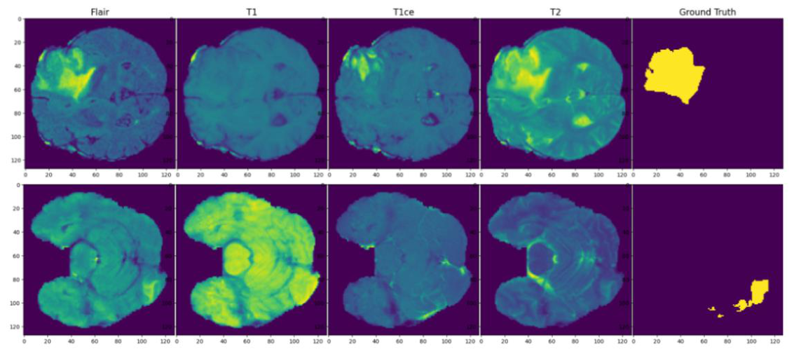
Figure 2.
The 1×64×64 Flair medical images generated by the SCGAN proposed in this paper through interpolation of the two feature inputs—shape and colour.
Figure 2.
The 1×64×64 Flair medical images generated by the SCGAN proposed in this paper through interpolation of the two feature inputs—shape and colour.
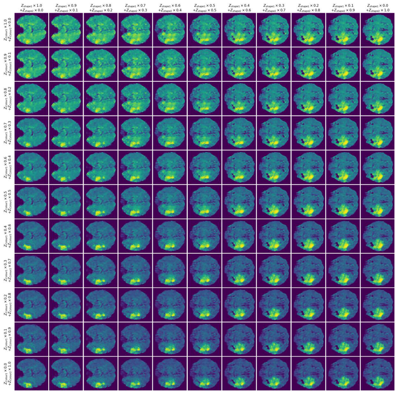
Figure 3.
Circularity Semantic Index of Latent Feature Vector Components.
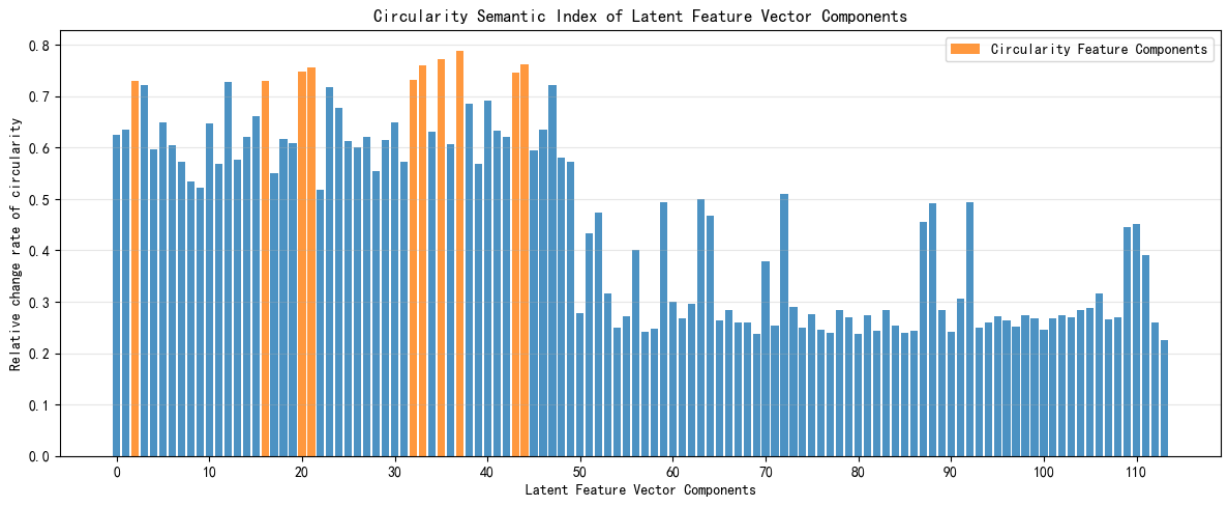
Figure 4.
Brightness Semantic Index of Latent Feature Vector Components.
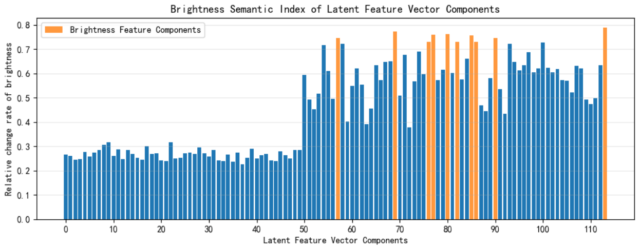
Figure 5.
Comparison between the original image and the image obtained by modifying 10 selected decoupled components of the circularity latent vector.
Figure 5.
Comparison between the original image and the image obtained by modifying 10 selected decoupled components of the circularity latent vector.
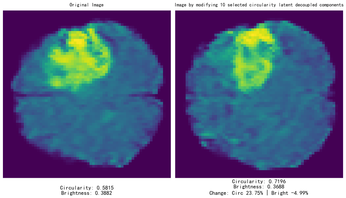
Figure 6.
Comparison between the original image and the image obtained by modifying 10 selected decoupled components of the brightness latent vector.
Figure 6.
Comparison between the original image and the image obtained by modifying 10 selected decoupled components of the brightness latent vector.
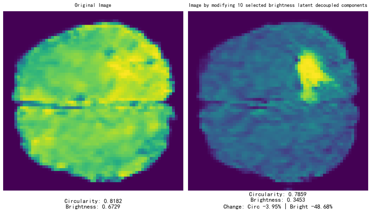
Figure 7.
Framework of SCGAN-MultiJNet.
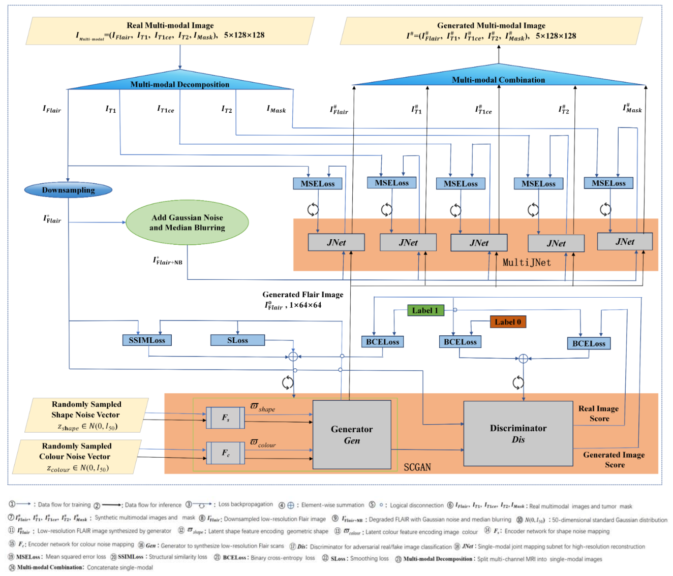
Figure 9.
Discriminator Architecture of SCGAN.
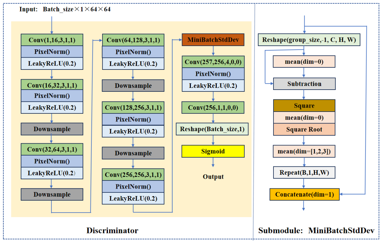
Figure 10.
JNet Architecture.
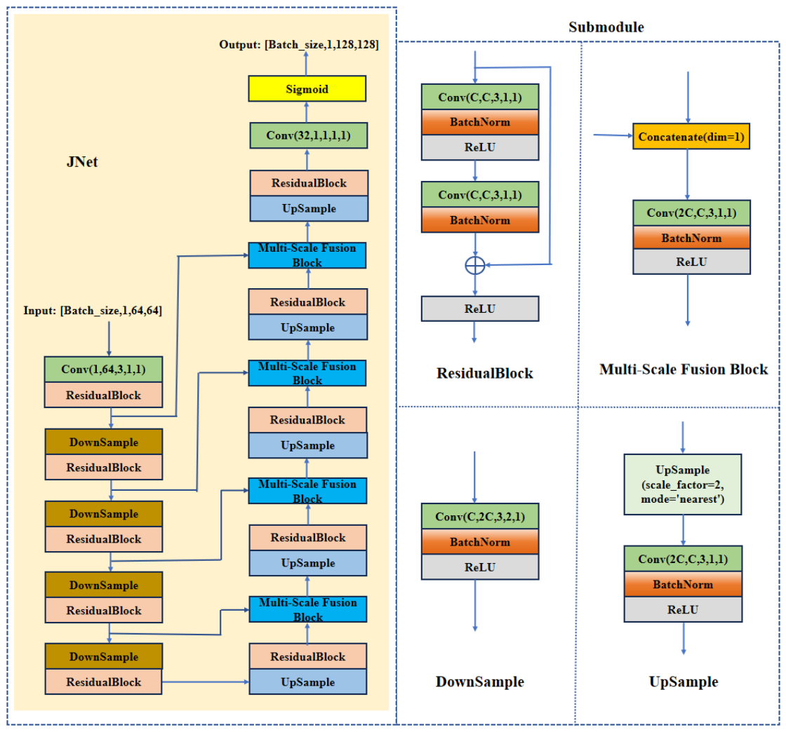
Figure 11.
Comparison of Original Flair Images in R64 and Blurred Flair Images in R64+NB .
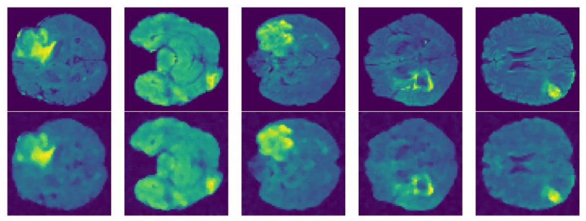
Figure 12.
Flair Images generation process visualization by SCGAN.
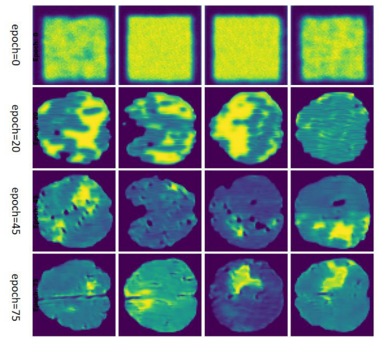
Figure 13.
Samples of Generative Multimodal Brain Tumor Images in the G.
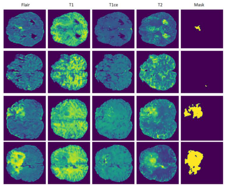
Figure 14.
Metrics of the U-Net on the Training Datasets in Case1.
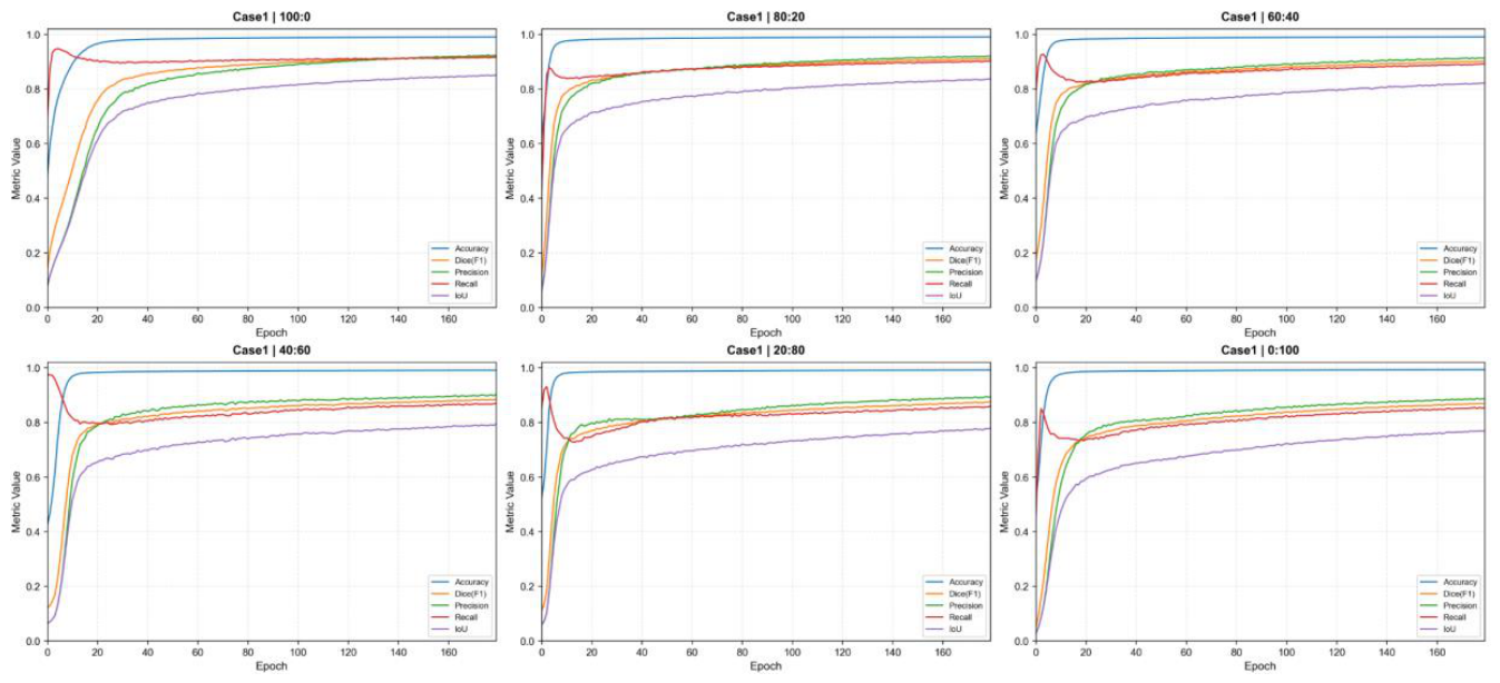
Figure 15.
The Curve Graph and Radar Chart of the Metrics on the Test Datasets Rtest in Case1.
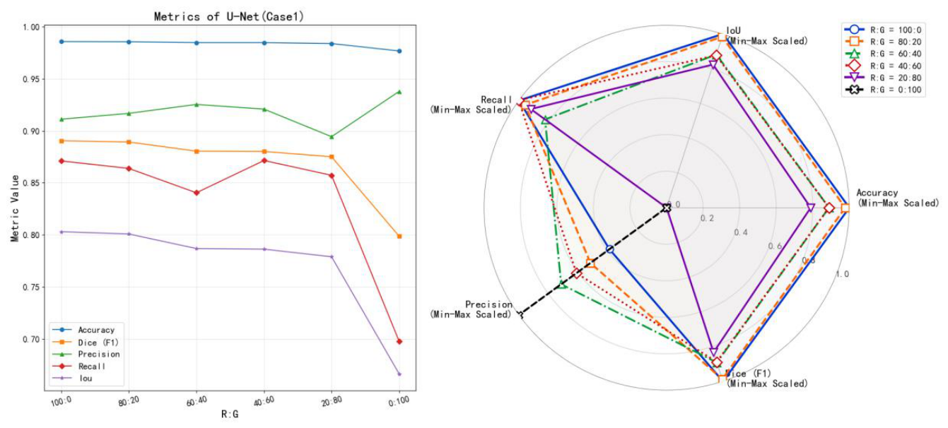
Figure 17.
The Curve Graph and Radar Chart of the Metrics on the Test Datasets Rtest in Case2.
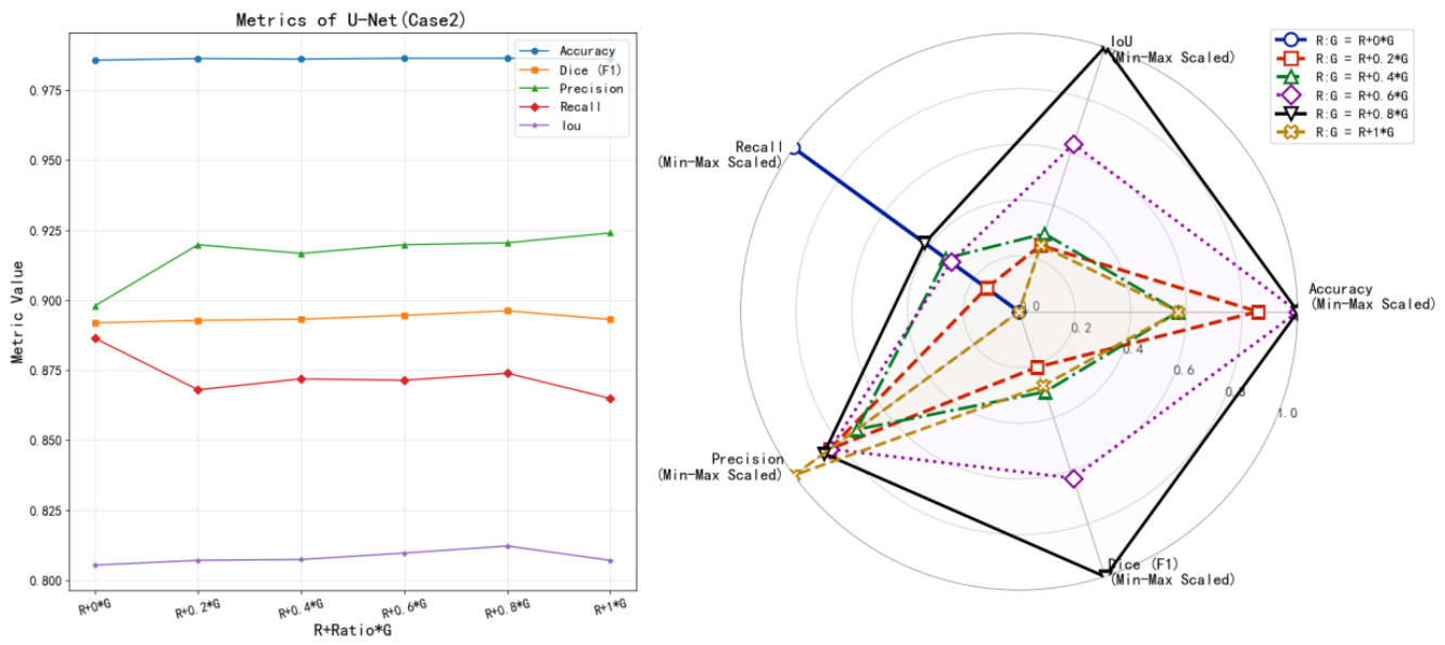
Figure 18.
Segmentation results on the Rtest under two scenarios: R and R+0.8*G.
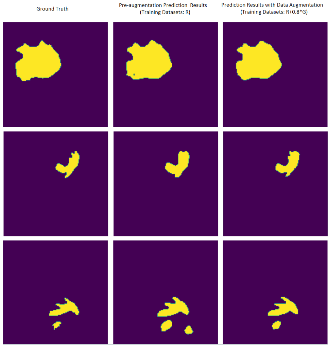
Figure 19.
Comparison of Metric Degradation across Eight Perturbations and Five Severity Grades.
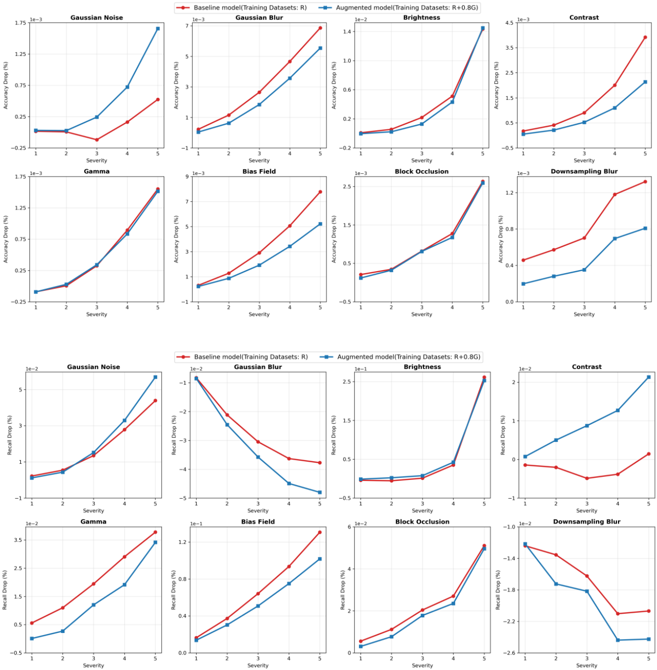
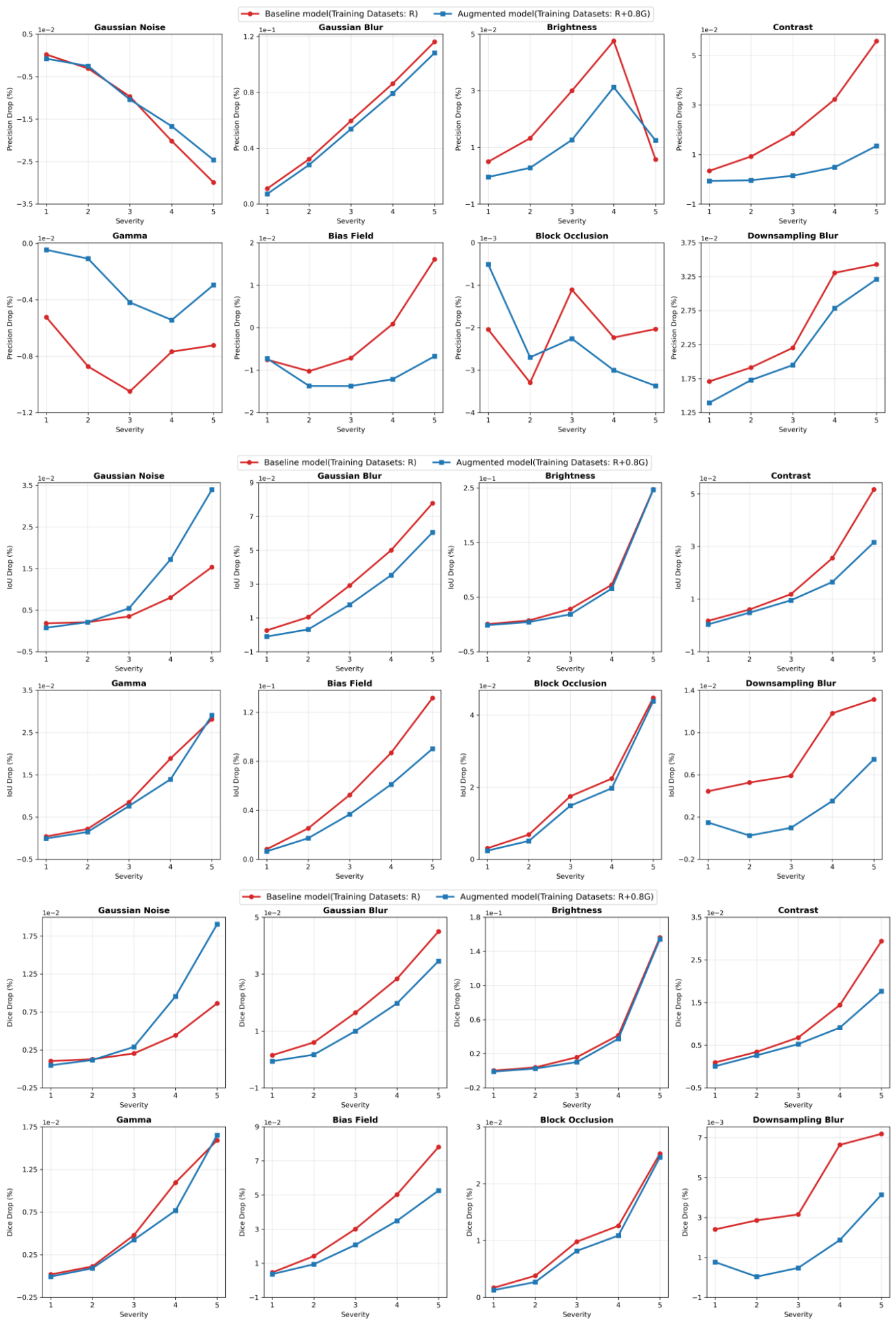
Table 1.
Parameter setting of SCGAN-MultiJNet.
| Parameter | Value | Parameter | Value |
| Number of iterations of SCGAN | 300 | Learning rate of Generator | 2e-05 |
| Batch size of SCGAN | 32 | Learning rate of Discriminator | 2e-05 |
| Number of iterations of JNet | 600 | Learning rate of JNet | 1e-05 |
| Batch size of JNet | 32 | Betas in AdamW or Adam | (0.9,0.999) |
Table 2.
Ablation Experiment Results.
| Synthetic images | Group | Configuration | FID (↓) | IS (↑) | PSNR (↑) | SSIM (↑) | MMD (↓) |
| 64×64 Flair images synthesized by SCGAN | A | Baseline: Backbone + BCELoss | 50.5578 | 1.6780 ± 0.0335 | 14.0217 | 0.2662 | 0.1798 |
| B | A + CFIConvLayer | 44.9116 | 1.6832 ± 0.0346 | 14.4482 | 0.2800 | 0.1658 | |
| C | B+SSIMLoss | 52.3539 | 2.0836 ± 0.0478 | 14.3284 | 0.2785 | 0.1315 | |
| D | C+SLoss | 8.9837 | 1.5215 ± 0.0288 | 14.1220 | 0.2762 | 0.0759 | |
| SCGAN-MultiJNet | A0 | Baseline:A+Upsample(Bilinear) | 64.5534 | 1.5443± 0.0241 | 14.1274 | 0.3399 | 0.5201 |
| A1 | A + JNet | 12.4144 | 1.2919± 0.0148 | 13.5370 | 0.2991 | 0.1433 | |
| B0 | A1+ CFIConvLayer | 48.8585 | 1.6326± 0.0351 | 13.8774 | 0.3054 | 0.1681 | |
| C0 | B0+SSIMLoss | 29.0166 | 1.7208± 0.0596 | 13.8679 | 0.3126 | 0.1334 | |
|
D0 (OursFull) |
C0+SLoss | 59.2537 | 2.0050± 0.0378 | 13.6335 | 0.3062 | 0.1574 |
* All experiments use GAN backbone, tested on synthetic Flair MRI.
Table 4.
Metrics of Segmentation Network U-Net on Rtest in Case2.
| R+ratio*G | Accuracy | Dice | Precision | Recall | IoU |
| R+0*G | 0.9857 | 0.8919 | 0.8980 | 0.8864 | 0.8054 |
| R+0.2*G | 0.9863 | 0.8928 | 0.9198 | 0.8680 | 0.8071 |
| R+0.4*G | 0.9861 | 0.8932 | 0.9167 | 0.8719 | 0.8074 |
| R+0.6*G | 0.9864 | 0.8946 | 0.9198 | 0.8714 | 0.8097 |
| R+0.8*G | 0.9864 | 0.8962 | 0.9205 | 0.8739 | 0.8122 |
| R+1*G | 0.9861 | 0.8931 | 0.9240 | 0.8649 | 0.8071 |
Table 7.
Metrics of Segmentation Network U-Net on BraTS2025-SSA-Data in Case2.
| R+ratio*G | Accuracy | Dice | Precision | Recall | IoU |
| R+0*G | 0.9631 | 0.6856 | 0.5901 | 0.8342 | 0.5275 |
| R+0.2*G | 0.9666 | 0.6980 | 0.6318 | 0.7940 | 0.5401 |
| R+0.4*G | 0.9621 | 0.6786 | 0.5887 | 0.8138 | 0.5171 |
| R+0.6*G | 0.9665 | 0.6952 | 0.6324 | 0.7853 | 0.5375 |
| R+0.8*G | 0.9623 | 0.6745 | 0.5902 | 0.8016 | 0.5130 |
| R+1*G | 0.9563 | 0.6387 | 0.5444 | 0.7894 | 0.4752 |
Disclaimer/Publisher’s Note: The statements, opinions and data contained in all publications are solely those of the individual author(s) and contributor(s) and not of MDPI and/or the editor(s). MDPI and/or the editor(s) disclaim responsibility for any injury to people or property resulting from any ideas, methods, instructions or products referred to in the content. |
© 2026 by the authors. Licensee MDPI, Basel, Switzerland. This article is an open access article distributed under the terms and conditions of the Creative Commons Attribution (CC BY) license (http://creativecommons.org/licenses/by/4.0/).
Copyright: This open access article is published under a Creative Commons CC BY 4.0 license, which permit the free download, distribution, and reuse, provided that the author and preprint are cited in any reuse.


