
Submitted:
09 July 2026
Posted:
13 July 2026
You are already at the latest version
Abstract
Forest understory vegetation contributes to aboveground and belowground carbon budgets and affects terrestrial ecosystem function, yet quantifying understory biomass at large spatial scales is difficult. Increasingly, forest management operations are aided by unmanned aerial vehicles (UAVs) that collect imagery and airborne light detection and ranging (LiDAR) data, potentially providing a dataset for understory monitoring. In this study, we evaluated the suitability of two different remote sensing datasets (A and B) for predicting understory biomass amounts (field average of 2 Mg ha-1) using five different machine learning models. We compared (1) Acquisition A LiDAR and multispectral data, (2) Acquisition A multispectral data only, (3) Acquisition B SfM photogrammetry point cloud and multispectral data, and (4) Acquisition B multispectral data only. Remotely sensed data were temporally linked to ground plots in open post-harvest conditions, where we employed a method for quick in-field biomass estimation via calibrated photos. Our best model was a stochastic gradient boosting model built with LiDAR and multispectral data (testing R2=0.43, training R2=0.67). The multispectral-only model from Acquisition A performed similarly (testing R2=0.44, training R2=0.53), despite larger bias in shaded areas, suggesting an alternative streamlined method for creating wall-to-wall estimates. Structure-for-motion was unfit for modeling biomass under all tested conditions, indicating the importance of data acquisition and post-processing. Our study provides a novel framework for evaluating low-volume understory biomass efficiently and creating landscape scale predictions using limited ground measurements and remotely sensed data.
Keywords:
remote sensing
; forest
; understory
; biomass
; machine learning
; stochastic gradient boosting
; structure-from-motion photogrammetry
; multispectral imagery
; early-seral
1. Introduction
The early-seral stage, characterized by a flush of rapid understory growth, can produce rival biomass amounts compared to forests [1] and play an important role in forest carbon budgets. Shrubs typically expand horizontally more rapidly than trees, as they have weaker apical dominance and thus higher leaf area and solar capture in early stand development [2], and provide more detrital carbon during this period [1]. Initial understory vegetation can influence forest development pathways and contribute to carbon storage over a longer timeframe [3]. Dense understory environments can inhibit seedling regeneration that result in prolonged open canopy conditions [4]. Some forest managers intentionally aim to create this extended open-canopy condition to increase forest structural diversity, provide forage for critical wildlife species, and promote culturally important species [5]. Tracking and monitoring vegetation in post-harvest conditions is essential to understanding forest dynamics and management options.
Understory biomass estimates involve destructive sampling or equations built with vegetation biometric data like percentage cover and plant height [6], requiring numerous in-field hours, and yet result in limited geographic inference. Remote sensing techniques offer an opportunity to quantify understory biomass at a scale that is meaningful to forest managers and researchers [7]. However, remotely sensed monitoring of post-disturbance vegetation in forested systems—especially small shrubs—has been limited. Technologies that accurately measure total aboveground biomass (AGB), principally dominated by overstory trees, have limited capability to quantify understory conditions [8]. Aerial LiDAR effectively captures the structure and height of dominant overstory trees. However, occlusion by the overstory prevents or greatly reduces the LiDAR pulses reaching the understory thus limiting inference in the understory [9]. LiDAR sensors can greatly underestimate the height of short and dense vegetation [10]. Satellite imagery has been successfully linked to total AGB [11]—and in open canopy conditions, shrub biomass [12]—but spatial resolution limits fine-scale estimates.
For short and low density vegetation in open young forests, conditions may be most similar to an agricultural field where remote sensing is used to monitor crop height, cover, and biomass [13,14], as well as detect weeds [15,16]. For these studies, crop biomass is a key indicator [17] and can be of interest as a proxy for crop yield [18], crop growth [19], drought-tolerant genotypes [20], production efficiency [21], and plant physiology [22]. Remotely sensed biomass estimation performance varies with vegetation growth structure [17], phenological stage [23], study environment [24] and different crop species [25,26] and among studies of the same species. As an example, for predicting sorghum biomass, model performance ranges from 0.11 R2 [20] to 0.89 R2 [27]. At the low end of biomass values, there can be additional error [25]. Numerous factors may influence model performance including equipment selection, sample size, and acquisition timing.
A variety of methods have been used to map understory biomass in forested systems. For example, aerial LiDAR data acquisitions, paired with photo-based understory cover board estimates, have been used to visually measure understory and predict vegetation structure (R2 = 0.44) [28]. Shrestha et al. (2021) used oven-dried understory mass measurements and a LiDAR sensor affixed to an unmanned aerial vehicle (UAV) to effectively quantify understory biomass in open conditions in the southeast United States (R2 = 0.51) [29]. Due to the common issue of understory occlusion with aerial data acquisitions, ground level remotely sensed data are collected to increase measurement precision [30]. Terrestrial Laser Scanning (TLS) offers close-proximity, high-resolution data from a horizontal rather than vertical vantage point and has been used in conjunction with aerial LiDAR to predict horizontal vegetation cover with a testing accuracy of 85% [31]. Similar terrestrial approaches using close-range photogrammetry with a GoPro resulted in poor total plot biomass estimates (R2 = 0.08 to 0.21) but predictions were improved when the lowest stratum of vegetation was removed (R2 = 0.74 to 0.85) [32]. These ground-based methods require special and potentially expensive remote sensing data collection campaigns that are not typical of forest management operations.
Building on this body of work, this study aims to further explore remote sensing datasets to quantify understory biomass using datasets that may already be routinely collected to assist forest managers. Increasingly, precision forest management operations and decision-making are aided by UAVs, which offer information at stand and large spatial scales including: tree detection and inventory; biomass and volume estimates; pest, disease, and invasive species detection; and conservation and restoration modeling [33,34]. Unlike other remote sensing methods, UAVs offer flexible acquisition timing, high-density point clouds, and high spatial resolution [35]. These acquisitions allow for relatively low-cost and replicable measurement and analysis of experimental treatments compared to expansive field plots. UAVs may be affixed with a LiDAR sensor, or more typically for forest management, just a multispectral or red, green, blue (RGB) camera. Camera imagery can be stitched together to create structure-from-motion (SfM) photogrammetric point clouds that can be analyzed using the same techniques used for LiDAR point clouds [35]. Zhang et al. (2022) used a low-flying drone and SfM to predict understory vegetation biomass based on a canopy height model. These techniques can have utility for certain forestry questions but lack of clarity about tradeoffs can make a single approach challenging to select. This study aims to explore the utility of several remote sensing datasets which are most collected by forest managers, to test quantification of understory biomass, shortly after harvest when biomass is relatively low.
The understory calculations are part of a larger experiment called the T3 Watershed Experiment, a 20,000-acre operational-scale experiment in the Olympic Experimental State Forest (OESF), Washington, U.S.A., aimed at expanding forest management options through the implementation of novel forest treatments. Several prescriptions within this experiment include a variable retention harvest followed by planting in ways that encourage and extend the early-seral forest stage, where understory biomass and species diversity can flourish [5]. Understory responses to these treatments have implications for co-benefits such as carbon sequestration, ungulate habitat and forage, and presence of culturally important species. A major goal of our study is to create baseline understory biomass estimates immediately post-harvest, upon which future work within the T3 Watershed Experiment can be built. Due to the operational-scale nature of the experiment, relying only on ground measurements is too time consuming and costly, leading us to use a remote sensing-based approach. A challenge for this goal is that baseline conditions at the study sites require modeling only very small amounts of understory (field measurements averaged 2 Mg ha-1), placing additional pressure on the remote sensing technology to capture sufficient information for accurate quantification.
Machine learning models can leverage remote sensing datasets to produce predictions that capture complex and non-linear relationships with less sensitivity to noise than conventional regression-based methods [36]. For predicting total AGB—not just the understory—non-parametric machine learning models are often employed, such as k-nearest neighbor, artificial neural networks, support vector machine, random forest, gradient boosting, and maximum entropy [37]. These machine learning methods offer tradeoffs in performance versus explainability of the model, as well as handling small datasets and noise [38]. Nevertheless, when comparing model performance, data type and quality can matter more than model selection in overall model performance [39].
For our study, we have two remotely sensed datasets: Acquisition A—UAV acquired LiDAR and multispectral imagery collected in 2024, and Acquisition B—UAV SfM photogrammetry and multispectral imagery collected in 2025. We compared model performance for (1) Acquisition A LiDAR and multispectral data, (2) Acquisition A multispectral data only, (3) Acquisition B SfM photogrammetry point cloud and multispectral data, and (4) Acquisition B multispectral data only. By pairing these remotely sensed datasets with photo-based understory ground plot measurements, our study aims to answer the following questions:
1. How do remote sensing approaches—UAV LiDAR with multispectral imagery, UAV SfM photogrammetry with multispectral imagery, and multispectral imagery alone—compare in their ability to predict understory biomass?
2. How and under what conditions can remote sensing aid in measuring understory biomass and novel treatment effectiveness?
3. Which machine learning model provides the most accurate predictions of understory biomass in open post-harvest conditions?
We seek to answer these questions while prioritizing feasibility and repeatability for researchers and managers in terms of available data and resources.
2. Materials and Methods
2.1. Study Area
The Olympic Peninsula lies in the northwest portion of Washington state (WA), U.S.A. The western portion of the Olympic Peninsula is characterized by temperate rainforests, which are predominantly wet, evergreen, and coniferous. Our study was conducted across two experimental sites on land managed by the Washington Department of Natural Resources (DNR) and within the Olympic Experimental State Forest (OESF) on the Olympic Peninsula: (1) the T3 Watershed Experiment mostly within the Hoh and Clearwater river watersheds, and (2) the Ethnoforestry field trials study site near La Push, WA (Figure 1.). Mean annual temperature in this region is 10.4 °C (14.9 °C for May–September), and average annual precipitation is 2959 mm (average of 90 mm for May–September) [40].
2.1.1. T3 Watershed Experiment Study Site
This study evaluates post-harvest conditions on three separate treatments that are part of the larger T3 Watershed Experiment: Variable Density Planting (VDP), Complex Early Seral (CES), and Polyculture (Poly). All T3 Watershed Experimental treatment units were harvested in 2024–2025 with various silvicultural designs [41]. Woody debris from the harvests were left on site. Pre-harvest conditions for the study sites were dominated by a dense western hemlock (Tsuga heterophylla (Raf.) Sarg.)/Douglas-fir (Pseudotsuga menziesii (Mirb.) Franco) overstory. For the purposes of this study, data collection was concentrated in open-canopy, post-harvest conditions and performed before herbicide applications and planting. In 2025, understory species composition included a mixture of (1) graminoids including velvet grass (Holcus lanatus L.), spike bentgrass (Agrostis exarata Trin.), and small flowered woodrush (Luzula parviflora (Ehrh.) Desv.); (2) diverse forbs including fragrant bedstraw (Galium triflorum Michx.), woodland ragwort (Senecio sylvaticus L.), Siberian springbeauty (Claytonia sibirica L.), redwood-sorrel (Oxalis oregana Nutt.), among others; and (3) a mixture of shrubs and ferns that were likely growing prior to timber harvest and survived, including salal (Gaultheria shallon), red huckleberry (Vaccinium parvifolium Sm.), western sword fern (Polystichum munitum (Kaulf.) C. Presl), and deer fern (Blechnum spicant (L.) Sm).
2.1.2. Ethnoforestry Field Trials Study Site
The Ethnoforestry field-trials study site is part of an existing randomized-block experiment to explore people-focused understory management [42]. Pre-harvest conditions for the study sites were dominated by a dense western hemlock/Douglas-fir overstory. The unit received a variable retention harvest in 2018, an herbicide application in August 2020, and planting from January to April 2021. Woody debris from the harvests were left on site. All units were planted with Douglas-fir and some units were also planted with red alder (Alnus rubra Bong.) as well as five understory species: whitebark raspberry (Rubus leucodermis Douglas ex Torr. & A. Gray), Roemer’s fescue (Festuca idahoensis Elmer spp. roemeri (Pavlick) S. Aiken), salmonberry (Rubus spectabilis Pursh), tall Oregon grape (Mahonia aquifolium (Pursh) Nutt.), and Nootka rose (Rosa nutkana C. Presl). In addition, understory regenerated naturally at this site over time with a similar mixture of graminoids, forbs, shrubs, and ferns as the units in the T3 Watershed Experiment. Dominant species at this site included hairy cat’s ear (Hypochaeris radicata L.), purple foxglove (Digitalis purpurea L.), spike bentgrass, velvetgrass, red elderberry (Sambucus racemosa L.), salal, several blackberry species (Rubus spp.), and many others.
2.2. Ground Data: Understory Biomass
Field measurements for understory biomass and species cover were collected on all study sites throughout the summers of 2024 and 2025. Understory biomass ground plots were measured by comparing the live understory biomass within the boundaries of the plot to a set of images in a Biomass Booklet created for this purpose [1]. This Booklet contains 31 images of 3 m x 3 m plots with associated dry weight values (Mg ha-1). Each image represents a different set of understory species with varying levels of biomass, identified through traditional methods of harvesting, drying, and weighing vegetation. Field crews matched plot images with conditions in ground plots to obtain biomass measurements (Figure 2.). For example, if ground plots were predominantly sword fern, crews looked for images within the Biomass Booklet that contained sword fern and selected the image that most closely aligned with ground conditions. In certain situations, no single photo would perfectly capture ground conditions. When matching to plots was difficult, measurements were taken from two sides of the plot and biomass averaged. In addition, when biomass photos were of similar species composition, but of a different density, additions or subtractions by percentage were determined. For example, if the ground plot contained twice as much sword fern as the best sword fern image within the booklet, the amount of biomass was double that of the associated image. Previous work with the Biomass Booklet evaluated observer bias across three separate visual estimates and found an 11% margin of error [1].
This method allows for fast ocular biomass estimates from plots of similar conditions and species distribution. To expand the condition options within the Biomass Booklet to better reflect early-seral conditions on all of the harvested study sites, plots outside the boundaries of the study area were photographed and received traditional biomass measurements: all vegetation within a 3 m x 3 m quadrat was removed, dried at 70 °C in ovens to a constant mass, and weighed. Total biomass (Mg ha-1) was calculated based on the dry weight values. New images and their associated biomass values were added to the Booklet to represent these early-seral conditions for future use.
Plot locations were distributed throughout the harvested units and stratified to capture the range of site conditions, while remaining limited to open-canopy areas. Biomass plots were georeferenced using a Javad Triumph 2, a survey grade GNSS receiver, so they could be spatially connected to remote sensing data (San Jose, CA, USA). Previous studies using post-processed Javad Triumph 2 data in Pacific Northwest forested conditions found a horizontal accuracy of 1.76 m, but this study found on average, slightly better results due to the open-canopy conditions [43]. Due to this slight offset, plot locations as recorded with the Javad Triumph 2 (Javad) were not perfectly aligned with remotely sensed data. A matching procedure outlined in Kruper, 2024 was used to spatially adjust plot locations, using the LiDAR data as the locational standard [44]. A series of LiDAR visible objects, such as stumps and downed logs, were used as reference points to adjust Javad plot locations to better match corresponding reference points in the LiDAR data. All adjustments were performed manually in ESRI ArcGIS Pro [45].
In most instances, plot locations were identified by two points at opposite corners to represent the full 3 m by 3 m square. When the two points were brought into ArcGIS, plot boundaries were not perfectly square. To resolve this and create a best match of in-field conditions, a center point between the two georeferenced points was generated and then a perfect 3 m x 3 m square was calculated around that center point. A small fraction of the ground plot data was taken with one central georeferenced point, for which the 3 m x 3 m square was calculated around that center point. For the Ethnoforestry field trials study site, this process was completed with 1.5 m x 1.5 m square plot boundaries, but these plots were related back to the biomass booklet at the 3 m x 3 m scale and therefore estimates were still at the 3 m x 3 m scale.
Some plots had to be removed from each dataset due to various georeferencing issues, such as a missing plot corner location. The final data included 191 ground plots measured in 2024 for Acquisition A (53 from the T3 Watershed Experiment and 138 from Ethnoforestry field trials), and 183 ground plots measured in 2025 for Acquisition B (25 from the T3 Watershed Experiment and 158 from Ethnoforestry field trials).
2.3. UAV Remotely Sensed Data
There were two separate remotely sensed data acquisitions across the study sites: Acquisition A in 2024 using UAV lidar and multispectral imagery, and Acquisition B in 2025 using UAV SfM photogrammetry and multispectral imagery (Table 1.). Remotely sensed data were matched with the ground data from the respective summers, creating two temporally linked datasets. For both acquisitions, ground data and remotely sensed data were separated in time by no more than two months. The two acquisitions had overlapping areas flown, including all the Ethnoforestry field trials study site, as well as non-overlapping additional study areas within the T3 Watershed Experiment for both flights (roughly half of the flight area of Acquisition A in 2024 was reflown for Acquisition B in 2025). For Acquisition A (UAV-LiDAR-Multispectral), remote sensing data were acquired for 91.1 hectares; for Acquisition B (UAV-SfM-Multispectral), remote sensing data was acquired for 215 hectares.
2.3.1. Acquisition A: UAV-LiDAR-Multispectral
In the summer of 2024, both UAV LiDAR and multispectral imagery data were collected by the natural resource consulting firm West Fork Environmental. LiDAR data were collected using a DJI Matrice 600 Pro UAV, with a Surveyor 32 LiDAR instrument, manufactured by LiDAR USA, with a Pandar XT32 scanner, made by Hesai. LiDAR flight height was 60 meters above ground level. Point density ranged from 402 to 702 points m-2. Multispectral imagery was acquired with a DJI Matrice 210 UAV, with an attached Altum-PT sensor made by Ag Eagle, formerly known as MicaSense. Imagery was collected at 120 meters above ground level. The Altum-PT sensor resolutions include 2064 × 1544 (3.2 MP per multispectral band), 4112 × 3008 (12 MP panchromatic), and 320 × 256 thermal infrared. For multispectral bands, the spectral ranges were the following: Blue (475 ± 16 nm), Green (560 ± 16 nm), Red (668 ± 14 nm), Red Edge (717 ± 12 nm), and Near-infrared (842 ± 57 nm). Processing was done with Agisoft Metashape. A calibration panel was used prior to takeoff and immediately following acquisition to calibrate the imagery in metashape. Photo alignment was performed with high accuracy, a no tie point limit, and 40,000 key points per photo limit. An orthomosaic surface was created using a DEM built within the Metashape software using the imagery dense point cloud. Spatial resolution for the imagery was 0.05 m.
A ground model was provided by the vendor using the following procedure and created with R programming software [46]: extract the lowest points in the LiDAR point cloud (from 0–0.15 m aboveground level); run the lidR classify_ground function using the Progressive Morphological Filter (PMF) option with a window sizes set to 3, 12 and 3 meters and linearly spaced elevation thresholds between 0.1 m and 1.5 m; and generate a DTM using a Triangulated Irregular Network interpolation method at a resolution of 0.5 m.
2.3.2. Acquisition B: UAV-SfM-Multispectral
In the summer of 2025, DNR used a DJI Mavic 3 Multispectral UAV to collect multispectral imagery and create a point cloud using SfM photogrammetry. The UAV was flown 122 m (400 ft) above ground level. For this acquisition, the RGB camera had a 20 MP resolution and a maximum image size of 5280 × 3956. The multispectral camera had a 5 MP effective resolution and captured four bands—Green (560 ± 16 nm), Red (650 ± 16 nm), Red Edge (730 ± 16 nm), and Near-infrared (860 ± 26 nm)—at a maximum image size of 2592 × 1944. Spatial resolution for the imagery was 0.04 m. Processing was done with Agisoft Metashape. Photo alignment was performed with high accuracy, a no tie point limit, and 40,000 key points per photo limit. The point cloud was created using densest possible point cloud without filtering noise. Point density ranged from 33 to 155 points m-2. For camera optimization, there was no adaptive camera model fitting, and fitting all other parameters (f, k1, k2, k3, k4, cx+cy, p1, p2, b1, b2). An orthomosaic surface was built from tie points, with a low poly surface count. Ground sampling distance varied but was on average ~2.5 cm per pixel.
Two different ground models were assessed for use: (1) an aerial LiDAR derived DTM from the Washington State LiDAR portal, and (2) a ground model generated from the SfM photogrammetric point cloud data, following the process outlined for the Acquisition A dataset. Option two, the generated ground model, was used for all further data processing and analysis because it resulted in better spatial alignment with the point cloud data.
2.4. Remotely Sensed Data Processing
All data processing was completed using R [46], and for the data processing stage, generative artificial intelligence [47] was used to explore functions, refine code, and debug code. The authors have reviewed and edited all outputs and take full responsibility for the content of this publication. Data processing was divided into two phases for both Acquisition A and B: (1) processing stand-scale data at the full geographic extent of the acquisitions to be used for model prediction, and (2) processing plot-scale data at the 3 m x 3 m (or 1.5 m x 1.5 m for Ethnoforestry field trials) scale for the creation of the models.
All data processing described in this section was the same for Acquisition A and B. Although the two acquisitions captured different multispectral bands, only the bands common to both were retained for the final models making the multispectral datasets equivalent in usable statistics. To make the two datasets match, statistics on multiband reflectance, panchromatic band and long-wave infrared were removed from Acquisition A, and statistics generated from the green multi-reflectance band and the red multi-reflectance band were removed from Acquisition B.
2.4.1. Stand Level Data Processing
The FUSION software (version 4.61) was used to process the Acquisition A LiDAR and Acquisition B SfM photogrammetric point cloud data [48]. Data for entire acquisition areas was run through the GridMetrics function to generate statistics on the point cloud. Points were normalized using the ground DTM. All points above zero were considered, ground points were ignored, a cell size of 3 m was used to match the ground plot size, and statistics were generated using the following height strata (meters above ground): 0.5, 1.0, 1.5, 2.0, 2.5, 3.0, 3.5.
For image processing, composite images were created following Xie et al. (2018). The following images were used in the analysis: RGB, False Color Near-Infrared (NIR), False Color Red Edge, Normalized Difference Vegetation Index (NDVI) using NIR and Red, NDVI using NIR and Red Edge, Modified Simple Ratio (MSR) using NIR and Red, MSR using NIR and Red Edge, Chlorophyll Index (CI) using NIR and Green, CI using NIR and Red Edge, NDVI using NIR, and weighted Red + Red Edge, MSR using NIR and weighted Red and Red Edge, Chlorophyll Index using NIR and weighted Red and Red Edge.
The aggregate function within Spatial Data Analysis (terra) package within R studio [50] was used to extract statistics at a 3 m resolution for all image layers. The following statistics were generated for each 3 m section of each composite image: max, min, mean, standard deviation (sd), 25th quantile, 75th quantile and coefficient of variation. The results of this stand level processing were a series of files containing statistics for all flown units at a 3 m x 3 m scale to match the scale of ground plots.
2.4.2. Plot Level Data Processing
Plot level data processing matched as much as possible the stand level data processing. The georeferenced and adjusted 3 m × 3 m ground (1.5 m x 1.5 m for Ethnoforestry field trials) plot locations were used to extract statistical information from all remotely sensed datasets, with point-based statistics generated using the FUSION software. First, LiDAR and SfM point cloud data were clipped to plot locations using the PolyClipData function. Plot elevations were normalized using the ClipData function and the ground DTM. This output was fed to the CloudMetrics function using parameters that matched the GridMetrics call applied to stand-level data; statistics were generated for height strata at 0.5 m increments from 0.5 to 3.5 m above ground.
For image processing at the plot level, data for each georeferenced plot location was extracted from all of the generated composite images using the extract function within the terra package, producing the same statistics as the aggregate function noted above: max, min, mean, standard deviation (sd), 25th quantile, 75th quantile and coefficient of variation.
2.4.3. Data Cleaning
Plot-scale statistics for the point clouds and multispectral imagery were joined for model building. Datasets created with Acquisition A and B were compared so that only shared columns across the two datasets were kept (330 columns for each dataset), making differences in multispectral bands available across the acquisitions irrelevant. Certain columns contained many NA values due to statistics being generated for height thresholds that the low-lying vegetation did not reach. For example, if the generated statistic was “standard deviation for all returns between 2.5 and 3 m”, but vegetation within the plot did not reach that height, then an “NA” value would be generated. “NA” values were then replaced with zeros for columns where no data values should logically be zero, such as point cloud statistics on counts or proportion. Subsequently, all columns with greater than 30% “NA” values were removed; this threshold was chosen because it was a natural breakpoint in the column-wise distribution of “NA” values. After removing these columns, 0.04% of the remaining values were “NA.” These remaining missing values were estimated using soft imputation, an iterative matrix completion algorithm that repeatedly computes a soft-thresholded Singular Value Decomposition based on the observed values until convergence. This was implemented using the softImpute package in R using a rank threshold of 10 [51,52]. Next, columns with a variance lower than 0.01 were dropped and highly correlated columns were filtered using the findCorrelation function in the caret R package [53]. Of the predictors that had a correlation higher than 0.95, the predictor that was more highly correlated with the entire dataset was dropped.
This resulted in 188 available predictors: 59 variables from the point cloud data and 129 variables from the multispectral imagery data. A full list of variables used in model building is available in the Appendix (Table A1). Broadly, major categories of variables that were culled based on criteria listed in the methods section include: all point cloud intensity metrics, metrics related to points in certain elevation strata where there were insufficient points, multispectral metrics that were only available with one acquisition but not the other, and multispectral metrics that were highly correlated.
The data were split into training and testing data, 80% train and 20% test, randomized across all samples (n=152 for A and n=146 for B). Predictor variables were mean-centered and scaled to unit variance using statistics derived from the training data, and the same transformations were applied to the corresponding test datasets. We then subset the 129 multispectral columns from each dataset and saved them separately, leaving us with four datasets for model building: (1) Acquisition A LiDAR and multispectral data, (2) Acquisition A multispectral data only, and (3) Acquisition B SfM photogrammetry point cloud and multispectral data, and (4) Acquisition B multispectral data only.
2.5. Machine Learning Models
Five machine learning models were fit to each of the four datasets: random forest (rf), stochastic gradient boosting (gbm), extreme gradient boosting (xgbTree), k-nearest neighbors algorithm (knn), and generalized linear model (glmnet). Model fitting and hyperparameter tuning was performed on all models using the caret package, using 5-fold cross-validation repeated 3 times in the training data [53]. All hyperparameter combinations, with final hyperparameter choices, were applied to all 4 datasets and are available in the Appendix (Table A2.). A small feed-forward neural network with two hidden layers was also implemented and tuned. However, it is omitted because it showed signs of significant overfitting, which can be expected in this use case due to limited and highly variable data. All models were fit to maximize the coefficient of determination, and this value as well as RMSE were computed.
2.6. Prediction
Stand-scale data were filtered and cleaned, following the same process as the plot level data. Data were scaled using statistics derived from the training dataset. The two best models were used to predict understory biomass (Mg ha-1) across all available stands. Ground data were collected in open-canopy conditions, so areas with existing canopy cover were removed from understory biomass totals for each experimental unit. Removal of these values was done using the mask function in the terra package, in which tree polygons generated in FUSION were buffered, unioned and then masked from the final predictive raster. In addition, ArcGIS was used to draw freehand polygons around heavily shaded regions and were also removed from the final prediction rasters. Prediction totals were generated using the global function in the terra package.
3. Results
3.1. Model Results
3.1.1. Model Performance
The predictive performance of all machine learning models built with Acquisition A (LiDAR-multispectral and multispectral only) was superior to that of all models built with Acquisition B (SfM-multispectral and multispectral only) (Figure 3). The best models were the stochastic gradient boosting models from the Acquisition A dataset, with the highest coefficients of determination and lowest RMSE values (LiDAR-multispectral: R2 = 0.43, RMSE = 0.76 Mg ha-1, relative error = 0.46; multispectral only: R2= 0.44, RMSE = 0.75 Mg ha-1, relative error = 0.47). Acquisition A random forest models also performed comparably but tended to be overfit evident by the high training coefficients of determination, and much lower testing coefficients of determination (LiDAR-multispectral: R2=0.39, RMSE = 0.78 Mg ha-1, relative error = 0.48).
For Acquisition B, all tested machine learning models were overfit, determined similarly by high training R2 values and low testing R2 values, indicating that the mean of the data would create a better prediction than these models. Visual inspection of Acquisition B SfM point cloud suggests poor spatial registration in the imagery contributed to poor model performance.
All tested models predicted higher values where trees created shade in the imagery, but this tendency was more extreme with the multispectral only models. Although Acquisition A multispectral-only model resulted in better model statistics than Acquisition A LiDAR and multispectral model, the multispectral-only model predicted higher biomass values overall, and upon visual inspection, seemed to overpredict in these shaded regions. All models also predicted high biomass values in leave-tree zones, where trees were left after harvest. Ground plots were not taken under existing canopy, nor were they stratified to include areas that would be shaded in the imagery, so predictions in these areas were outside the scope of the model capabilities and not considered in final stand biomass estimates (Figure 4.). Biomass estimates produced from our best model, Acquisition A LiDAR and multispectral model, for each stand can be found in Table 2.
3.1.2. Variable Importance Scores
The top five predictors for all created models were multispectral variables (Table 3.). Bands that were particularly important include red edge, MSR, CI using NIR and Red Edge, and NIR. These results indicate that for our tested models, LiDAR metrics were not as important as multispectral metrics.
4. Discussion
We connected ground-based understory biomass estimates to two distinct UAV data acquisitions to identify feasibility of using these common datasets to predict wall-to-wall understory biomass for forest management and research. Three research questions guided the analysis:
- How do remote sensing approaches—UAV LiDAR with multispectral imagery, UAV SfM photogrammetry with multispectral imagery, and multispectral imagery alone—compare in their ability to predict understory biomass?;
- How and under what conditions can remote sensing aid in measuring understory biomass and novel treatment effectiveness?; and
- Which machine learning model provides the most accurate predictions of understory biomass in open post-harvest conditions?
In addition, this work sought to document baseline conditions for experimental units as part of a larger long-term experiment.
Through the combination of UAV LiDAR, multispectral imagery and ground biomass plots, we calculated coarse estimates of biomass across the entire stand, functional for estimating low, medium, and high biomass amounts. We created a pathway for limited in-field data collection using a set of calibrated photos called the Biomass Booklet, that can be linked to commonly acquired forestry remote sensing data with very little additional field work. Furthermore, we identified the weaknesses in the approach—even in open-canopy conditions with high spatial resolution UAV-based data, SfM photogrammetry alone was ill-suited for this type of research using the hardware and software as we applied it. The combination of low biomass values and poor spatial registration likely resulted in relatively low estimation performance for all models tested.
4.1. How do Remote Sensing Approaches—UAV LiDAR with Multispectral Imagery, UAV SfM Photogrammetry with Multispectral Imagery, and Multispectral Imagery Alone—Compare in Their Ability to Predict Understory Biomass?
Acquisition A was able to generate predictions for understory biomass across management units, but model estimation performance was relatively low (LiDAR-multispectral: R2 = 0.43). Although other researchers have had better modeling success with biomass estimates when average biomass levels are significantly higher [54,55], our study reflects variability in the field and the challenges of measuring and predicting extremely low biomass values [20]. Our model results from Acquisition A suggest that comparable predictions can be generated using multispectral data alone, significantly reducing data processing time compared to processing both imagery and LiDAR data. Upon visual inspection of the wall-to-wall estimates, the multispectral-only model may be less useful in areas with leave trees, where shade may reduce model performance. Based on our variable importance scores, the multispectral statistics were of highest utility for all our models, which we suspect were effectively capturing presence and absence of low-lying vegetation. Our study site also had a high degree of woody slash, which at times, was taller than the vegetation, and could be affecting our model performance as an additional layer of occlusion and source of error in point filtering [56]. When vegetation height is a greater determinant for total volume and therefore total biomass, and overtopping the coarse woody debris, we suspect that the LiDAR-based statistics will have higher relevance and our model performance may improve.
In contrast, Acquisition B, using SfM and multispectral imagery, was unfit for this type of analysis under all tested conditions, which is not particularly surprising considering SfM is a technique with mixed results for low-lying vegetation [57]. We analyzed this dataset with two different ground models: one using the public access DTM from the WA State LiDAR portal and one with a ground model generated from the SfM point cloud. SfM photogrammetry extracts keypoints from individual photos, finds keypoint matches between photos, and uses algorithms to reconstruct feature and camera locations [58]. Through visual inspection of the point cloud with both ground models, we suspect this dataset had poor spatial registration between photos, leading to floating points and a high degree of noise. This noise may be tolerable for some types of analysis, but due to our small plot size (3 m x 3 m) and minimal low-lying modeled vegetation, vegetation size (branch and foliage) likely made image matching challenging. Moreover, photos must capture all vegetation angles to generate sufficient signatures. Through comparing the multispectral-only models from Acquisition A and B, we can see that the quality of the Acquisition B multispectral-only data was also poor, meaning that this issue likely extended to the post-processing and stitching together of the orthomosaic imagery. Cunliffe et al. (2016) used SfM motion photogrammetry to model biomass at a fine scale, but they employed systematically acquired convergent image data, nadir image data, and high-precision ground-control points, which required multiple flights over the same area. In our case, post-processing of the Acquisition B dataset was done following standard protocol for forest management where a high level of optimization is not needed. A lack of precision in feature matching within Acquisition B likely caused poor performance in the corresponding models.
Differences in model performance between the two Acquisitions may also be attributed to equipment. For example, Acquisition A multispectral imagery was acquired with an Altum-PT sensor, whereas Acquisition B used the Mavic 3 Multispectral camera. Product performance differences for the cameras, as well as differences in position and altitude sensing instrumentation, may account for at least part of the performance discrepancies.
4.2. How and Under What Conditions can Remote Sensing Aid in Measuring Understory Biomass and Novel Treatment Effectiveness?
Our study benefited from numerous advantages that made low biomass understory estimates possible, despite understory predictions being more challenging to generate than upper canopy predictions [8]. First, we had temporally linked remote sensing and ground datasets that were no more than two months apart in time. Understory biomass can grow quickly, so timing of data acquisition influences matching of on-the-ground conditions with remote sensing signatures, and discrepancies in data collection timing can complicate study outcomes [25]. Second, knowing that understory biomass is difficult to measure when tall trees are present, we focused our analysis on open-canopy conditions. Because our study was conducted on the Olympic Peninsula, where forests are extremely dense, plots under existing canopy cover were unlikely to generate reasonable model predictions. Based on other studies in more open forests [60], we suspect this process could be replicated in other locations with some existing tree cover, such as low-density dry forests. Third, our remotely sensed data set was extremely high density (33–702 points m-2), which would be achievable only with a UAV and professional-grade equipment.
A key component of this work that made this remote sensing study feasible was the Biomass Booklet, a set of calibrated photos for quick visual understory biomass estimates. This tool allowed for minimal ground crew work: crews were tasked to take plots in designated areas, they established georeferenced plot information, measured a 3 m x 3 m square, and then chose an estimated biomass value. Georeferencing can be completed once for multiple plots; crews measured Javad locations once and subsequently measured the distance and azimuth to this Javad location for multiple plot locations, which can then be reconstructed using R programming to create a map of all plot locations. Therefore, the in-field process can be fast and efficient—expanding this operation to include more ground points may improve model performance with little additional time. However, these biomass values are inherently subjective estimates, and they have the potential for large error or bias. Models generated from these estimates can be expected to have lower performance than using actual dried and weighed biomass estimates. For our purposes, we are hoping to track broad trends in understory change between novel harvest regimes, so absolute accuracy is less important than tiered (relative) values that indicate whether management activity is warranted.
Despite these advantages, our model performance in terms of R2 is lower compared to other field-based studies of understory biomass, most of which measure orders of magnitude more understory biomass than our study. Our study had an average biomass of 1.3 Mg ha-1 for 2024 field measurements compared to 8.2 Mg ha-1 [55] and 26 Mg ha-1 [54]. Because of the plants that we were measuring and predicting, our study may be comparable to those in agricultural fields, where model performance is highly variable [20]. Moreover, in accordance with agricultural research, a typical practice in this field is to eliminate points close to the ground that capture rocks or raised soil that may create additional noise in the data [61]. This can be done through reassigning points between 0 and 5 cm to a height of 0 cm [61]. We tested whether removing these low-lying points improved our model performance for models built with Acquisition A, but we found no improvement, concluding that ground noise was not affecting model performance.
Additional estimation error may be due to the complexity of growth forms and habits of early-seral plants. For example, sprouting species (e.g., bigleaf maple) may generate numerous small-diameter stems that cumulatively account for a substantial amount of biomass but may be challenging to measure or estimate individually [62], potentially contributing to field-data bias. Ruderal plants can produce high densities of biomass rapidly, and intermediate deciduous shrubs have branches that rapidly spread foliage laterally. In contrast, conifers take years to develop a full array of needle age classes, are mostly determinant (growth is fixed before bud breaks), and have crown shapes that limit outward growth. Differences in growth forms and respective differences in biomass accumulation, may make accurate predictions of the early-seral environment more challenging than a conifer-dominated system.
4.3. Which Machine Learning Model Provides the Most Accurate Predictions of Understory Biomass in Open Post-Harvest Conditions?
For Acquisition A, the stochastic gradient boosting model had the best predictive capacity and lowest error rate. Although the random forest model was a close second in model fit, R2 values were higher in the training versus testing dataset, indicating that these models were overfit to the training dataset. This issue was exacerbated for Acquisition B, indicating the models were mostly fit to noise in the data rather than distinguishing a true pattern. Ultimately, data quality (determined by acquisition and post-processing) was much more important than model selection, with Acquisition A models being superior to Acquisition B models under all conditions.
Future work will explore replicating these methods with larger vegetation and greater biomass quantities, which may improve model performance because vegetation will more often overtop slash, be more easily captured by multispectral cameras, and have larger three-dimensional form that can be measured with LiDAR height and structure metrics. A minimum vegetation biomass may exist for this analysis in which vegetation is robust and visible but not yet producing closed-canopy occlusion. For future use of the Biomass Booklet, observer bias could be reduced by (1) setting up calibration plots for crews, and (2) including more than two observers for each plot and keeping estimates independent.
5. Conclusions
Our study tested model capability to predict understory biomass for two datasets across open-canopy experimental units. We concluded that remotely sensed data quality is more important than model selection and that acquisition methods, including post-processing procedures, can dictate feasibility of this type of study. Poor spatial registration can result in poor-performing models, particularly for a study such as this with a very fine spatial scale. However, the combination of high-quality UAV-acquired multispectral imagery and LiDAR produced a model that can predict tiered understory biomass values at a scale that is useful to forest managers. Multispectral imagery was particularly useful for model building, constituting the top predictors for the best-performing models. In open canopy conditions, multispectral-only models could allow for relatively accurate understory biomass predictions at lower cost compared to more expensive LiDAR-based approaches. Future work should explore whether combining the Biomass Booklet, a set of calibrated photos for measuring understory biomass, with other remote sensing methods, such as convergent image data, improves model accuracy. This framework should also be employed in areas with denser understory to assess whether model performance improves when more vegetation is present.
Author Contributions
Conceptualization, R.M., B.B., S.D., and C.B.; methodology, S.D., A.K. and R.M.; formal analysis, A.M. and S.D.; writing—original draft preparation, S.D.; writing—review and editing, S.D., R.M., A.M., B.B., C.B., A.K.,G.E.; visualization, S.D.; supervision, R.M., B.B., G.E.; project administration, B.B. and C.B.; funding acquisition, B.B. All authors have read and agreed to the published version of the manuscript.
Funding
This research was funded by a State of Washington legislative proviso to the Washington Department of Natural Resources and University of Washington’s Olympic Natural Resource Center. Added support came from the University of Washington’s Center for Sustainable Forestry at Pack Forest.
Data Availability Statement
Data used in this study are available upon request.
Acknowledgments
We would like to thank and acknowledge Chris Erickson, West Fork Environmental and Miles Micheletti for data acquisition and answering related questions. Thank you to Teodora Minkova, research and monitoring lead for the Olympic Experimental State Forest for supporting this work. We also acknowledge the hard work from two Olympic Natural Resource Center Field Crews to establish and measure ground plots. During the preparation of this manuscript/study, the author(s) used ChatGPT (version GPT-4o), for the purposes of exploring functions, refining code, and debugging code. The authors have reviewed and edited the output and take full responsibility for the content of this publication.
Conflicts of Interest
The authors declare no conflict of interest.
Appendix A
Appendix A.1

Table A1.
This table shows the final variables used in model building. For both Acquisition A and B, one model was built with both point cloud and multispectral data and one model was built with multispectral data only.
Table A1.
This table shows the final variables used in model building. For both Acquisition A and B, one model was built with both point cloud and multispectral data and one model was built with multispectral data only.
| Variable Type for Predictive Modeling | List of Predictors |
|---|---|
| Point Cloud Variables Used | Return.1.count.above.0.00, Elev.minimum, Elev.maximum, Elev.mode, Elev.variance, Elev.CV, Elev.IQ, Elev.skewness, Elev.kurtosis, Elev.MAD.median, Elev.MAD.mode, Elev.L1, Elev.L2, Elev.L3, Elev.L4, Elev.L.CV, Elev.L.skewness, Elev.L.kurtosis, Elev.P01, Elev.P05, Elev.P10, Elev.P20, Elev.P25, Elev.P30, Elev.P40, Elev.P80, Elev.P99, Canopy.relief.ratio, Percentage.all.returns.above.0.00, X.All.returns.above.0.00.....Total.first.returns., Percentage.all.returns.above.mean, Percentage.all.returns.above.mode, X.All.returns.above.mode.....Total.first.returns., First.returns.above.mean, First.returns.above.mode, All.returns.above.mean, All.returns.above.mode, Total.first.returns, Total.all.returns, Elev.strata..below.0.50..total.return.count, Elev.strata..below.0.50..return.proportion, Elev.strata..below.0.50..min, Elev.strata..below.0.50..max, Elev.strata..below.0.50..mean, Elev.strata..below.0.50..mode, Elev.strata..below.0.50..median, Elev.strata..below.0.50..stddev, Elev.strata..below.0.50..CV, Elev.strata..below.0.50..skewness, Elev.strata..below.0.50..kurtosis, Elev.strata..0.50.to.1.00..total.return.count, Elev.strata..0.50.to.1.00..return.proportion, Elev.strata..1.00.to.1.50..total.return.count, Elev.strata..1.00.to.1.50..return.proportion, Elev.strata..1.50.to.2.00..total.return.count, Elev.strata..1.50.to.2.00..return.proportion, Elev.strata..2.00.to.2.50..total.return.count, Elev.strata..2.00.to.2.50..return.proportion, Profile.area |
| Multispectral Variables Used | blue_reflectance_band_1_max, blue_reflectance_band_1_min, blue_reflectance_band_1_mean, blue_reflectance_band_1_sd, blue_reflectance_band_1_q25, blue_reflectance_band_1_q75, blue_reflectance_band_1_coef_var, cigreen_band_1_max, cigreen_band_1_min, cigreen_band_1_mean, cigreen_band_1_sd, cigreen_band_1_q25, cigreen_band_1_q75, cigreen_band_1_coef_var, cirededge_band_1_max, cirededge_band_1_min, cirededge_band_1_sd, cirededge_band_1_q25, cirededge_band_1_q75, cirededge_band_1_coef_var, ciredrededge_band_1_max, ciredrededge_band_1_min, ciredrededge_band_1_mean, ciredrededge_band_1_sd, ciredrededge_band_1_q25, ciredrededge_band_1_q75, ciredrededge_band_1_coef_var, green_reflectance_band_1_max, green_reflectance_band_1_min, green_reflectance_band_1_mean, green_reflectance_band_1_sd, green_reflectance_band_1_q25, green_reflectance_band_1_q75, green_reflectance_band_1_coef_var, msr_band_1_max, msr_band_1_min, msr_band_1_mean, msr_band_1_sd, msr_band_1_q25, msr_band_1_q75, msr_band_1_coef_var, msrrededge_band_1_min, msrrededge_band_1_mean, msrrededge_band_1_sd, msrrededge_band_1_q25, msrrededge_band_1_q75, msrrededge_band_1_coef_var, msrredrededge_band_1_min, msrredrededge_band_1_mean, msrredrededge_band_1_sd, msrredrededge_band_1_q25, msrredrededge_band_1_coef_var, NIR_band_1_coef_var, NIR_band_2_coef_var, NIR_band_3_coef_var, nir_re_g_band_1_max, nir_re_g_band_1_min, nir_re_g_band_1_mean, nir_re_g_band_1_sd, nir_re_g_band_1_q25, nir_re_g_band_1_q75, nir_re_g_band_1_coef_var, nir_re_g_band_2_coef_var, nir_re_g_band_3_coef_var, nir_reflectance_band_1_max, nir_reflectance_band_1_min, nir_reflectance_band_1_mean, nir_reflectance_band_1_sd, nir_reflectance_band_1_q25, nir_reflectance_band_1_q75, nir_reflectance_band_1_coef_var, nvdinir_band_1_max, nvdinir_band_1_min, nvdinir_band_1_mean, nvdinir_band_1_sd, nvdinir_band_1_q25, nvdinir_band_1_q75, nvdinir_band_1_coef_var, nvdirededge_band_1_max, nvdirededge_band_1_min, nvdirededge_band_1_mean, nvdirededge_band_1_sd, nvdirededge_band_1_q25, nvdirededge_band_1_q75, nvdirededge_band_1_coef_var, nvdiredrededge_band_1_min, nvdiredrededge_band_1_mean, nvdiredrededge_band_1_sd, nvdiredrededge_band_1_q25, nvdiredrededge_band_1_q75, nvdiredrededge_band_1_coef_var, red_reflectance_band_1_max, red_reflectance_band_1_min, red_reflectance_band_1_mean, red_reflectance_band_1_sd, red_reflectance_band_1_q25, red_reflectance_band_1_q75, red_reflectance_band_1_coef_var, rededge_band_1_max, rededge_band_1_min, rededge_band_1_sd, rededge_band_1_q75, rededge_band_1_coef_var, rededge_band_2_coef_var, rededge_band_3_coef_var, rededge_reflectance_band_1_max, rededge_reflectance_band_1_min, rededge_reflectance_band_1_mean, rededge_reflectance_band_1_sd, rededge_reflectance_band_1_q25, rededge_reflectance_band_1_q75, rededge_reflectance_band_1_coef_var, RGB_band_1_max, RGB_band_1_sd, RGB_band_1_q25, RGB_band_1_q75, RGB_band_1_coef_var, RGB_band_2_max, RGB_band_2_min, RGB_band_2_sd, RGB_band_2_q25, RGB_band_2_q75, RGB_band_2_coef_var, RGB_band_3_max, RGB_band_3_min, RGB_band_3_sd, RGB_band_3_q25, RGB_band_3_q75, RGB_band_3_coef_var. |
Table A2.
All hyperparameter combinations and final hyperparameter choices for all machine learning models tested with the four datasets: Acquisition A (A) LiDAR and multispectral (MS), A MS only, Acquisition B (B) SfM and MS, B MS.
Table A2.
All hyperparameter combinations and final hyperparameter choices for all machine learning models tested with the four datasets: Acquisition A (A) LiDAR and multispectral (MS), A MS only, Acquisition B (B) SfM and MS, B MS.
| Model | Parameter | Values Tested | A Full | B Full | A MS | B MS |
|---|---|---|---|---|---|---|
| GLMNet | Alpha (mixing percentage) | seq(0, 1, 0.1) | 1 | 1 | 1 | 1 |
| Lambda (regularization strength) | 10seq(-5, -1, 0.1) | 0.1 | 0.0126 | 0.1 | 0.0126 | |
| KNN | k (number of neighbors) | 1:15 | 15 | 3 | 14 | 3 |
| RF | mtry (number randomly selected predictors) | 2, 3, 4, 5, 13, 62, 94 | 3 | 62 | — | — |
| mtry (number randomly selected predictors) | 2, 3, 4, 5, 11, 43, 64, 129 | — | — | 5 | 129 | |
| GBM | n.trees (boosting iterations) | 250, 500, 750, 1000, 1250, 1500 | 250 | 500 | 500 | 1000 |
| interaction.depth (maximum tree depth) | 1, 2, 3 | 3 | 1 | 1 | 1 | |
| shrinkage (learning rate) | 0.01, 0.05, 0.1 | 0.01 | 0.05 | 0.01 | 0.1 | |
| n.minobsinnode (minimum terminal node size) | 5, 10 | 10 | 5 | 10 | 10 | |
| xgbTree | eta (learning rate) | 0.3, 0.4 | 0.3 | 0.4 | 0.3 | 0.3 |
| max_depth (maximum tree depth) | 1, 2 | 1 | 1 | 1 | 1 | |
| subsample (subsample percentage) | 0.5, 0.75 | 0.75 | 0.5 | 0.75 | 0.75 | |
| nrounds (boosting iterations) | 50, 100 | 50 | 50 | 50 | 50 | |
| colsample_bytree (column subsample ratio) | 1 | 1 | 1 | 1 | 1 |
References
- Bormann, B.T.; Darbyshire, R.L.; Homann, P.S.; Morrissette, B.A.; Little, S.N. Managing Early Succession for Biodiversity and Long-Term Productivity of Conifer Forests in Southwestern Oregon. For. Ecol. Manag. 2015, 340, 114–125. [Google Scholar] [CrossRef]
- Cline, M.G. Apical Dominance. Bot. Rev. 1991, 57, 318–358. [Google Scholar] [CrossRef]
- Prescott, C.E.; Sajedi, T. The Role of Salal in Forest Regeneration Problems in Coastal British Columbia: Problem or Symptom? For. Chron. 2008, 84, 29–36. [Google Scholar] [CrossRef]
- Freund, J.A.; Franklin, J.F.; Larson, A.J.; Lutz, J.A. Multi-Decadal Establishment for Single-Cohort Douglas-Fir Forests. Can. J. For. Res. 2014, 44, 1068–1078. [Google Scholar] [CrossRef]
- Swanson, M.E.; Franklin, J.F.; Beschta, R.L.; Crisafulli, C.M.; DellaSala, D.A.; Hutto, R.L.; Lindenmayer, D.B.; Swanson, F.J. The Forgotten Stage of Forest Succession: Early-Successional Ecosystems on Forest Sites. Front. Ecol. Environ. 2011, 9, 117–125. [Google Scholar] [CrossRef]
- Paul, K.I.; Roxburgh, S.H.; Chave, J.; England, J.R.; Zerihun, A.; Specht, A.; Lewis, T.; Bennett, L.T.; Baker, T.G.; Adams, M.A.; et al. Testing the Generality of Above-Ground Biomass Allometry across Plant Functional Types at the Continent Scale. Glob. Change Biol. 2016, 22, 2106–2124. [Google Scholar] [CrossRef] [PubMed]
- Li, A.; Glenn, N.F.; Olsoy, P.J.; Mitchell, J.J.; Shrestha, R. Aboveground Biomass Estimates of Sagebrush Using Terrestrial and Airborne LiDAR Data in a Dryland Ecosystem. Agric. For. Meteorol. 2015, 213, 138–147. [Google Scholar] [CrossRef]
- Fernández-Guisuraga, J.M.; Suárez-Seoane, S.; Fernandes, P.M.; Fernández-García, V.; Fernández-Manso, A.; Quintano, C.; Calvo, L. Pre-Fire Aboveground Biomass, Estimated from LiDAR, Spectral and Field Inventory Data, as a Major Driver of Burn Severity in Maritime Pine (Pinus Pinaster) Ecosystems. For. Ecosyst. 2022, 9, 100022. [Google Scholar] [CrossRef]
- Hull, I.T.; Shipley, L.A. Testing the Ability of Airborne LiDAR to Measure Forage Resources for Wild Ungulates in Conifer Forests. J. For. 2019, 117, 492–503. [Google Scholar] [CrossRef]
- Streutker, D.R.; Glenn, N.F. LiDAR Measurement of Sagebrush Steppe Vegetation Heights. Remote Sens. Environ. 2006, 102, 135–145. [Google Scholar] [CrossRef]
- Khan, M.N.; Tan, Y.; Gul, A.A.; Abbas, S.; Wang, J. Forest Aboveground Biomass Estimation and Inventory: Evaluating Remote Sensing-Based Approaches. Forests 2024, 15, 1055. [Google Scholar] [CrossRef]
- Berner, L.T.; Jantz, P.; Tape, K.D.; Goetz, S.J. Tundra Plant Above-Ground Biomass and Shrub Dominance Mapped across the North Slope of Alaska. Environ. Res. Lett. 2018, 13, 35002. [Google Scholar] [CrossRef]
- Jimenez-Berni, J.A.; Deery, D.M.; Rozas-Larraondo, P.; Condon, A. (Tony) G.; Rebetzke, G.J.; James, R.A.; Bovill, W.D.; Furbank, R.T.; Sirault, X.R.R. High Throughput Determination of Plant Height, Ground Cover, and Above-Ground Biomass in Wheat with LiDAR. Front. Plant Sci. 2018, 9, 237. [Google Scholar] [CrossRef] [PubMed]
- Pittman, J.; Arnall, D.; Interrante, S.; Moffet, C.; Butler, T. Estimation of Biomass and Canopy Height in Bermudagrass, Alfalfa, and Wheat Using Ultrasonic, Laser, and Spectral Sensors. Sensors 2015, 15, 2920–2943. [Google Scholar] [CrossRef] [PubMed]
- Andújar, D.; Rueda-Ayala, V.; Moreno, H.; Rosell-Polo, J.R.; Escolá, A.; Valero, C.; Gerhards, R.; Fernández-Quintanilla, C.; Dorado, J.; Griepentrog, H.-W. Discriminating Crop, Weeds and Soil Surface with a Terrestrial LIDAR Sensor. Sensors 2013, 13, 14662–14675. [Google Scholar] [CrossRef] [PubMed]
- Shahbazi, N.; Ashworth, M.B.; Callow, J.N.; Mian, A.; Beckie, H.J.; Speidel, S.; Nicholls, E.; Flower, K.C. Assessing the Capability and Potential of LiDAR for Weed Detection. Sensors 2021, 21. [Google Scholar] [CrossRef] [PubMed]
- Poley, L.G.; McDermid, G.J. A Systematic Review of the Factors Influencing the Estimation of Vegetation Aboveground Biomass Using Unmanned Aerial Systems. Remote Sens. 2020, 12, 1052. [Google Scholar] [CrossRef]
- Walter, J.; Edwards, J.; McDonald, G.; Kuchel, H. Photogrammetry for the Estimation of Wheat Biomass and Harvest Index. Field Crops Res. 2018, 216, 165–174. [Google Scholar] [CrossRef]
- Cen, H.; Wan, L.; Zhu, J.; Li, Y.; Li, X.; Zhu, Y.; Weng, H.; Wu, W.; Yin, W.; Xu, C.; et al. Dynamic Monitoring of Biomass of Rice under Different Nitrogen Treatments Using a Lightweight UAV with Dual Image-Frame Snapshot Cameras. Plant Methods 2019, 15, 32. [Google Scholar] [CrossRef] [PubMed]
- Li, J.; Schachtman, D.P.; Creech, C.F.; Wang, L.; Ge, Y.; Shi, Y. Evaluation of UAV-Derived Multimodal Remote Sensing Data for Biomass Prediction and Drought Tolerance Assessment in Bioenergy Sorghum. Crop J. 2022, 10, 1363–1375. [Google Scholar] [CrossRef]
- Hiel, M.-P.; Barbieux, S.; Pierreux, J.; Olivier, C.; Lobet, G.; Roisin, C.; Garré, S.; Colinet, G.; Bodson, B.; Dumont, B. Impact of Crop Residue Management on Crop Production and Soil Chemistry after Seven Years of Crop Rotation in Temperate Climate, Loamy Soils. PeerJ 2018, 6, e4836. [Google Scholar] [CrossRef] [PubMed]
- Yuan, M.; Burjel, J.C.; Isermann, J.; Goeser, N.J.; Pittelkow, C.M. Unmanned Aerial Vehicle–Based Assessment of Cover Crop Biomass and Nitrogen Uptake Variability. J. Soil Water Conserv. 2019, 74, 350–359. [Google Scholar] [CrossRef]
- Moeckel, T.; Dayananda, S.; Nidamanuri, R.R.; Nautiyal, S.; Hanumaiah, N.; Buerkert, A.; Wachendorf, M. Estimation of Vegetable Crop Parameter by Multi-Temporal UAV-Borne Images. Remote Sens. 2018, 10, 805. [Google Scholar] [CrossRef]
- Mutanga Corresponding author, O.; Skidmore, A.K. Narrow Band Vegetation Indices Overcome the Saturation Problem in Biomass Estimation. Int. J. Remote Sens. 2004, 25, 3999–4014. [Google Scholar] [CrossRef]
- Prabhakara, K.; Hively, W.D.; McCarty, G.W. Evaluating the Relationship between Biomass, Percent Groundcover and Remote Sensing Indices across Six Winter Cover Crop Fields in Maryland, United States. Int. J. Appl. Earth Obs. Geoinf. 2015, 39, 88–102. [Google Scholar] [CrossRef]
- Grüner, E.; Astor, T.; Wachendorf, M. Biomass Prediction of Heterogeneous Temperate Grasslands Using an SfM Approach Based on UAV Imaging. Agronomy 2019, 9, 54. [Google Scholar] [CrossRef]
- Masjedi, A.; Crawford, M.M.; Carpenter, N.R.; Tuinstra, M.R. Multi-Temporal Predictive Modelling of Sorghum Biomass Using UAV-Based Hyperspectral and LiDAR Data. Remote Sens. 2020, 12. [Google Scholar] [CrossRef]
- Campbell, M.J.; Dennison, P.E.; Hudak, A.T.; Parham, L.M.; Butler, B.W. Quantifying Understory Vegetation Density Using Small-Footprint Airborne Lidar. Remote Sens. Environ. 2018, 215, 330–342. [Google Scholar] [CrossRef]
- Shrestha, M.; Broadbent, E.N.; Vogel, J.G. Using GatorEye UAV-Borne LiDAR to Quantify the Spatial and Temporal Effects of a Prescribed Fire on Understory Height and Biomass in a Pine Savanna. Forests 2021, 12, 38. [Google Scholar] [CrossRef]
- Li, S.; Wang, T.; Hou, Z.; Gong, Y.; Feng, L.; Ge, J. Harnessing Terrestrial Laser Scanning to Predict Understory Biomass in Temperate Mixed Forests. Ecol. Indic. 2021, 121, 107011. [Google Scholar] [CrossRef]
- Batchelor, J.L.; Hudak, A.T.; Gould, P.; Moskal, L.M. Terrestrial and Airborne Lidar to Quantify Shrub Cover for Canada Lynx (Lynx Canadensis) Habitat Using Machine Learning. Remote Sens. 2023, 15, 4434. [Google Scholar] [CrossRef]
- Cova, G.R.; Prichard, S.J.; Rowell, E.; Drye, B.; Eagle, P.; Kennedy, M.C.; Nemens, D.G. Evaluating Close-Range Photogrammetry for 3D Understory Fuel Characterization and Biomass Prediction in Pine Forests. Remote Sens. 2023, 15, 4837. [Google Scholar] [CrossRef]
- Dainelli, R.; Toscano, P.; Di Gennaro, S.F.; Matese, A. Recent Advances in Unmanned Aerial Vehicles Forest Remote Sensing—A Systematic Review. Part II: Research Applications. Forests 2021, 12, 397. [Google Scholar] [CrossRef]
- Adão, T.; Hruška, J.; Pádua, L.; Bessa, J.; Peres, E.; Morais, R.; Sousa, J. Hyperspectral Imaging: A Review on UAV-Based Sensors, Data Processing and Applications for Agriculture and Forestry. Remote Sens. 2017, 9, 1110. [Google Scholar] [CrossRef]
- Fernández-Guisuraga, J.M.; Calvo, L.; Suárez-Seoane, S. Monitoring Post-Fire Neighborhood Competition Effects on Pine Saplings under Different Environmental Conditions by Means of UAV Multispectral Data and Structure-from-Motion Photogrammetry. J. Environ. Manag. 2022, 305, 114373. [Google Scholar] [CrossRef] [PubMed]
- Thapa, B.; Lovell, S.; Wilson, J. Remote Sensing and Machine Learning Applications for Aboveground Biomass Estimation in Agroforestry Systems: A Review. Agrofor. Syst. 2023, 97, 1097–1111. [Google Scholar] [CrossRef]
- Tian, L.; Wu, X.; Tao, Y.; Li, M.; Qian, C.; Liao, L.; Fu, W. Review of Remote Sensing-Based Methods for Forest Aboveground Biomass Estimation: Progress, Challenges, and Prospects. Forests 2023, 14, 1086. [Google Scholar] [CrossRef]
- Lu, D.; Chen, Q.; Wang, G.; Liu, L.; Li, G.; Moran, E. A Survey of Remote Sensing-Based Aboveground Biomass Estimation Methods in Forest Ecosystems. Int. J. Digit. Earth 2016, 9, 63–105. [Google Scholar] [CrossRef]
- Almeida, D.R.A.; Broadbent, E.N.; Zambrano, A.M.A.; Wilkinson, B.E.; Ferreira, M.E.; Chazdon, R.; Meli, P.; Gorgens, E.B.; Silva, C.A.; Stark, S.C.; et al. Monitoring the Structure of Forest Restoration Plantations with a Drone-Lidar System. Int. J. Appl. Earth Obs. Geoinf. 2019, 79, 192–198. [Google Scholar] [CrossRef]
- PRISM Climate Group, Oregon State University PRISM Data Explorer 2026.
- Bormann, B.T.; Minkova, T.V.; Bobsin, C.; Devine, W.D.; Donato, D.C.; Slesak, R.; Ettl, G.; Alexander, K.; Churchill, D. The T3 Watershed Experiment Upland Silviculture Study Plan; Washington Department of Natural Resources, Forest Resources Division: Olympia, WA, 2022. [Google Scholar]
- Bobsin, C.R. Ethnoforestry and Adaptive Management: Generating New Pathways to Manage Forests on the Olympic Peninsula, WA; University of Washington Libraries: Seattle, 2023. [Google Scholar]
- McGaughey, R.J.; Ahmed, K.; Andersen, H.-E.; Reutebuch, S.E. Effect of Occupation Time on the Horizontal Accuracy of a Mapping-Grade GNSS Receiver under Dense Forest Canopy. Photogramm. Eng. Remote Sens. 2017, 83, 861–868. [Google Scholar] [CrossRef]
- Kruper, A. Western Redcedar on the Olympic Peninsula: Locating This Culturally, Economically, and Ecologically Important Species Using Remote Sensing Methodologies. In ProQuest Dissertations & Theses; 2024. [Google Scholar]
- ESRI ArcGIS Pro (Version 3.0.0) 2022.
- R Core Team R: A Language and Environment for Statistical Computing 2022.
- OpenAI ChatGPT (GPT-4o) [Large Language Model]. 2025.
- McGaughey, R. J. FUSION/LDV: Software for LIDAR Data Analysis and Visualization; U.S. Department of Agriculture, Forest Service, Pacific Northwest Research Station, 2024. [Google Scholar]
- Xie, Q.; Dash, J.; Huang, W.; Peng, D.; Qin, Q.; Mortimer, H.; Casa, R.; Pignatti, S.; Laneve, G.; Pascucci, S.; et al. Vegetation Indices Combining the Red and Red-Edge Spectral Information for Leaf Area Index Retrieval. IEEE J. Sel. Top. Appl. Earth Obs. Remote Sens. 2018, 11, 1482–1493. [Google Scholar] [CrossRef]
- Hijmans, R.J.; Brown, A.; Barbosa, M. Terra: Spatial Data Analysis; 2026. [Google Scholar]
- Hastie, T.; Mazumder, R.; Lee, J.; Zadeh, R. Matrix Completion and Low-Rank SVD via Fast Alternating Least Squares. J. Mach. Learn. Res. 2015, 16, 3367–3402. [Google Scholar] [PubMed]
- Mazumder, R.; Hastie, T.; Tibshirani, R. Spectral Regularization Algorithms for Learning Large Incomplete Matrices. J. Mach. Learn. Res. 2010, 11, 2287–2322. [Google Scholar] [PubMed]
- Kuhn, M. Building Predictive Models in R Using the Caret Package. J. Stat. Softw. 2008, 28, 1–26. [Google Scholar] [CrossRef]
- Alonzo, M.; Dial, R.J.; Schulz, B.K.; Andersen, H.-E.; Lewis-Clark, E.; Cook, B.D.; Morton, D.C. Mapping Tall Shrub Biomass in Alaska at Landscape Scale Using Structure-from-Motion Photogrammetry and Lidar. Remote Sens. Environ. 2020, 245, 111841. [Google Scholar] [CrossRef]
- Zhang, Y.; Onda, Y.; Kato, H.; Feng, B.; Gomi, T. Understory Biomass Measurement in a Dense Plantation Forest Based on Drone-SfM Data by a Manual Low-Flying Drone under the Canopy. J. Environ. Manag. 2022, 312, 114862. [Google Scholar] [CrossRef] [PubMed]
- Wing, B.M.; Ritchie, M.W.; Boston, K.; Cohen, W.B.; Gitelman, A.; Olsen, M.J. Prediction of Understory Vegetation Cover with Airborne Lidar in an Interior Ponderosa Pine Forest. Remote Sens. Environ. 2012, 124, 730–741. [Google Scholar] [CrossRef]
- Zahawi, R.A.; Dandois, J.P.; Holl, K.D.; Nadwodny, D.; Reid, J.L.; Ellis, E.C. Using Lightweight Unmanned Aerial Vehicles to Monitor Tropical Forest Recovery. Biol. Conserv. 2015, 186, 287–295. [Google Scholar] [CrossRef]
- Dandois, J.P.; Ellis, E.C. High Spatial Resolution Three-Dimensional Mapping of Vegetation Spectral Dynamics Using Computer Vision. Remote Sens. Environ. 2013, 136, 259–276. [Google Scholar] [CrossRef]
- Cunliffe, A.M.; Brazier, R.E.; Anderson, K. Ultra-Fine Grain Landscape-Scale Quantification of Dryland Vegetation Structure with Drone-Acquired Structure-from-Motion Photogrammetry. Remote Sens. Environ. 2016, 183, 129–143. [Google Scholar] [CrossRef]
- Olsoy, P.J.; Zaiats, A.; Delparte, D.M.; Germino, M.J.; Richardson, B.A.; Roser, A.V.; Forbey, J.S.; Cattau, M.E.; Caughlin, T.T. Demography with Drones: Detecting Growth and Survival of Shrubs with Unoccupied Aerial Systems. Restor. Ecol. 2024, 32, n/a. [Google Scholar] [CrossRef]
- Walter, J.D.C.; Edwards, J.; McDonald, G.; Kuchel, H. Estimating Biomass and Canopy Height With LiDAR for Field Crop Breeding. Front. Plant Sci. 2019, 10, 1145. [Google Scholar] [CrossRef] [PubMed]
- Matula, R.; Damborská, L.; Nečasová, M.; Geršl, M.; Šrámek, M. Measuring Biomass and Carbon Stock in Resprouting Woody Plants. PLoS ONE 2015, 10, e0118388. [Google Scholar] [CrossRef] [PubMed]
Figure 1.
Olympic Experimental State Forest study sites in WA were analyzed in this study: the Ethnoforestry field trials study site near La Push, WA (purple, top frame; 47.9071°N, 124.4750°W) and various harvested units part of a much larger 20,000-acre experiment called the T3 Watershed Experiment (orange, bottom frame; eastern most plot: 47.6451°N, 124.0955°W).
Figure 1.
Olympic Experimental State Forest study sites in WA were analyzed in this study: the Ethnoforestry field trials study site near La Push, WA (purple, top frame; 47.9071°N, 124.4750°W) and various harvested units part of a much larger 20,000-acre experiment called the T3 Watershed Experiment (orange, bottom frame; eastern most plot: 47.6451°N, 124.0955°W).
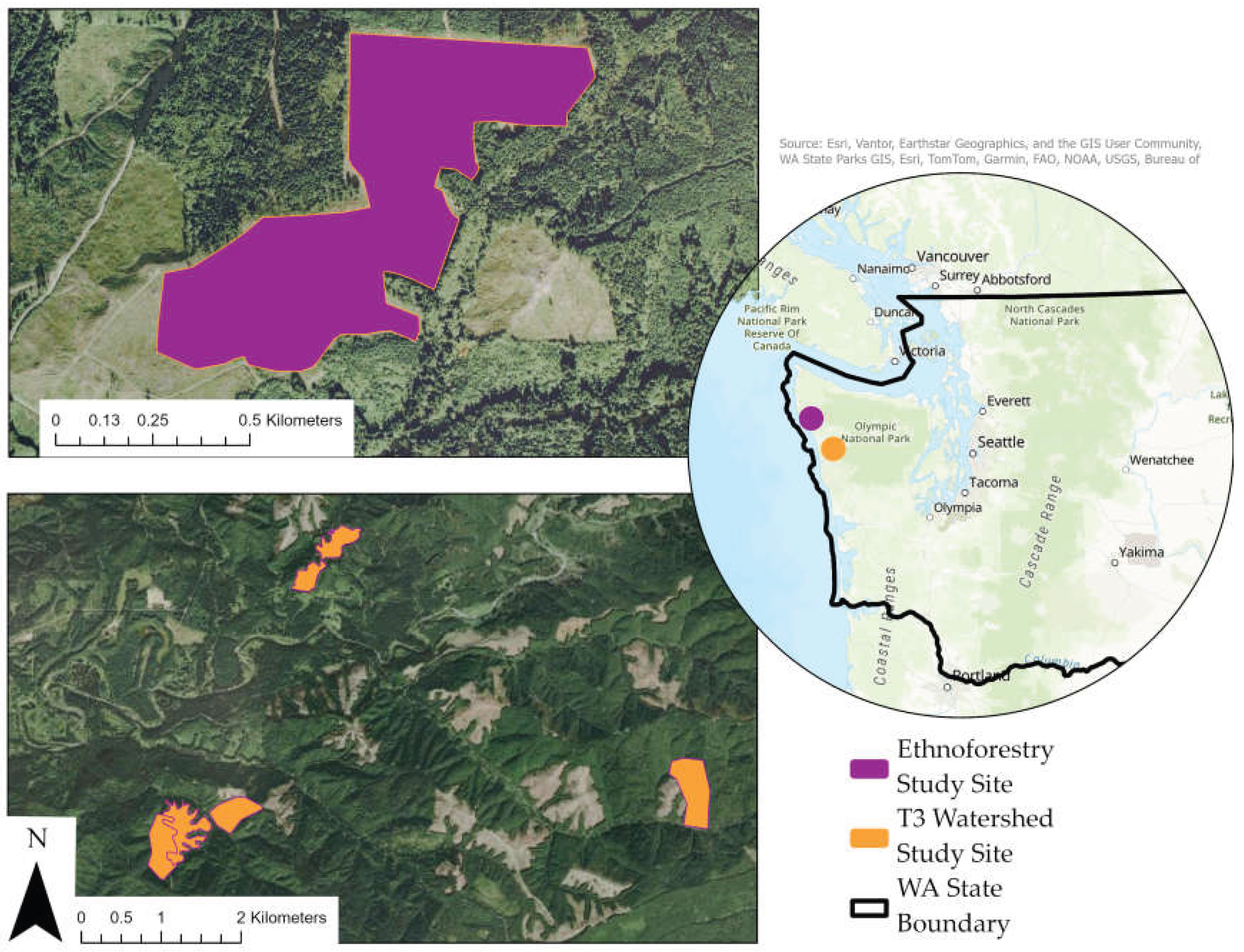
Figure 2.
An example of a calibrated photo from the Biomass Booklet, which contains a series of photos with corresponding biomass values. Text at the bottom of each image specifies dried weight for the vegetation in the photo and the corresponding dominant species in the plot, and photos are labeled for easy data entry (F2 label in the top right). Field crews matched 3 m x 3 m plot conditions with the best-fit photo to create quick ocular estimates that were then used to create our predictive model.
Figure 2.
An example of a calibrated photo from the Biomass Booklet, which contains a series of photos with corresponding biomass values. Text at the bottom of each image specifies dried weight for the vegetation in the photo and the corresponding dominant species in the plot, and photos are labeled for easy data entry (F2 label in the top right). Field crews matched 3 m x 3 m plot conditions with the best-fit photo to create quick ocular estimates that were then used to create our predictive model.
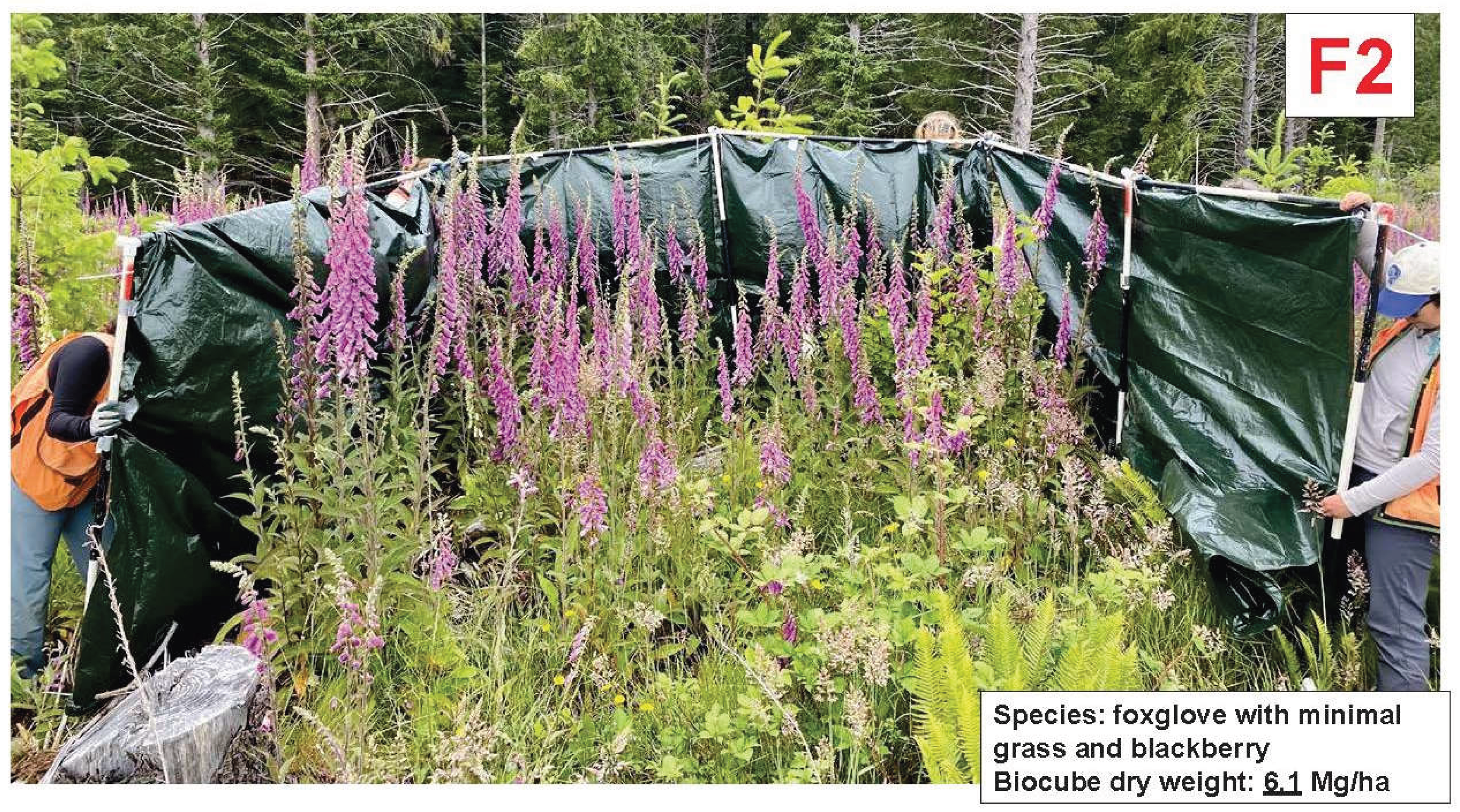
Figure 3.
Coefficient of determination (R2) training and testing data model results for Acquisition A and B. The following datasets were tested: (1) Acquisition A LiDAR and multispectral data, (2) Acquisition A multispectral data only, and (3) Acquisition B SfM photogrammetry point cloud and multispectral data, and (4) Acquisition B multispectral data only. The following models were trained and tested: k-nearest neighbors algorithm (knn), extreme gradient boosting (xgbTree), generalized linear model (glmnet), random forest (rf), and stochastic gradient boosting (gbm).
Figure 3.
Coefficient of determination (R2) training and testing data model results for Acquisition A and B. The following datasets were tested: (1) Acquisition A LiDAR and multispectral data, (2) Acquisition A multispectral data only, and (3) Acquisition B SfM photogrammetry point cloud and multispectral data, and (4) Acquisition B multispectral data only. The following models were trained and tested: k-nearest neighbors algorithm (knn), extreme gradient boosting (xgbTree), generalized linear model (glmnet), random forest (rf), and stochastic gradient boosting (gbm).
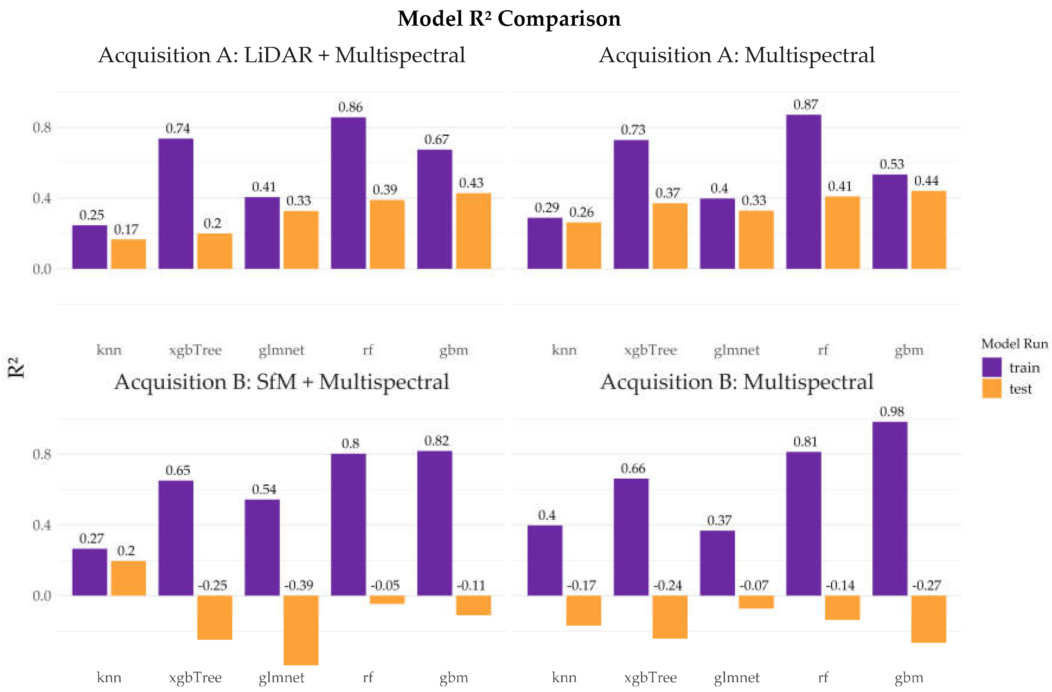
Figure 4.
Images are of the Variable Density Polyculture unit within the T3 Watershed Experiment. These four panels show the filtering process for generating wall-to-wall understory biomass predictions using our best performing model, the LiDAR and multispectral stochastic gradient boosting model built with Acquisition A. Panels are the following: i) Aerial image of harvested unit at time of data collection, ii) biomass predictions in Mg ha-1 of the entire unit, including areas outside of the scope of the model, such as shaded and closed canopy regions, iii) shaded and closed canopy regions removed from the final model predictions, iv) final model predictions to be used as baseline estimates for future experimental work and forest management decisions.
Figure 4.
Images are of the Variable Density Polyculture unit within the T3 Watershed Experiment. These four panels show the filtering process for generating wall-to-wall understory biomass predictions using our best performing model, the LiDAR and multispectral stochastic gradient boosting model built with Acquisition A. Panels are the following: i) Aerial image of harvested unit at time of data collection, ii) biomass predictions in Mg ha-1 of the entire unit, including areas outside of the scope of the model, such as shaded and closed canopy regions, iii) shaded and closed canopy regions removed from the final model predictions, iv) final model predictions to be used as baseline estimates for future experimental work and forest management decisions.
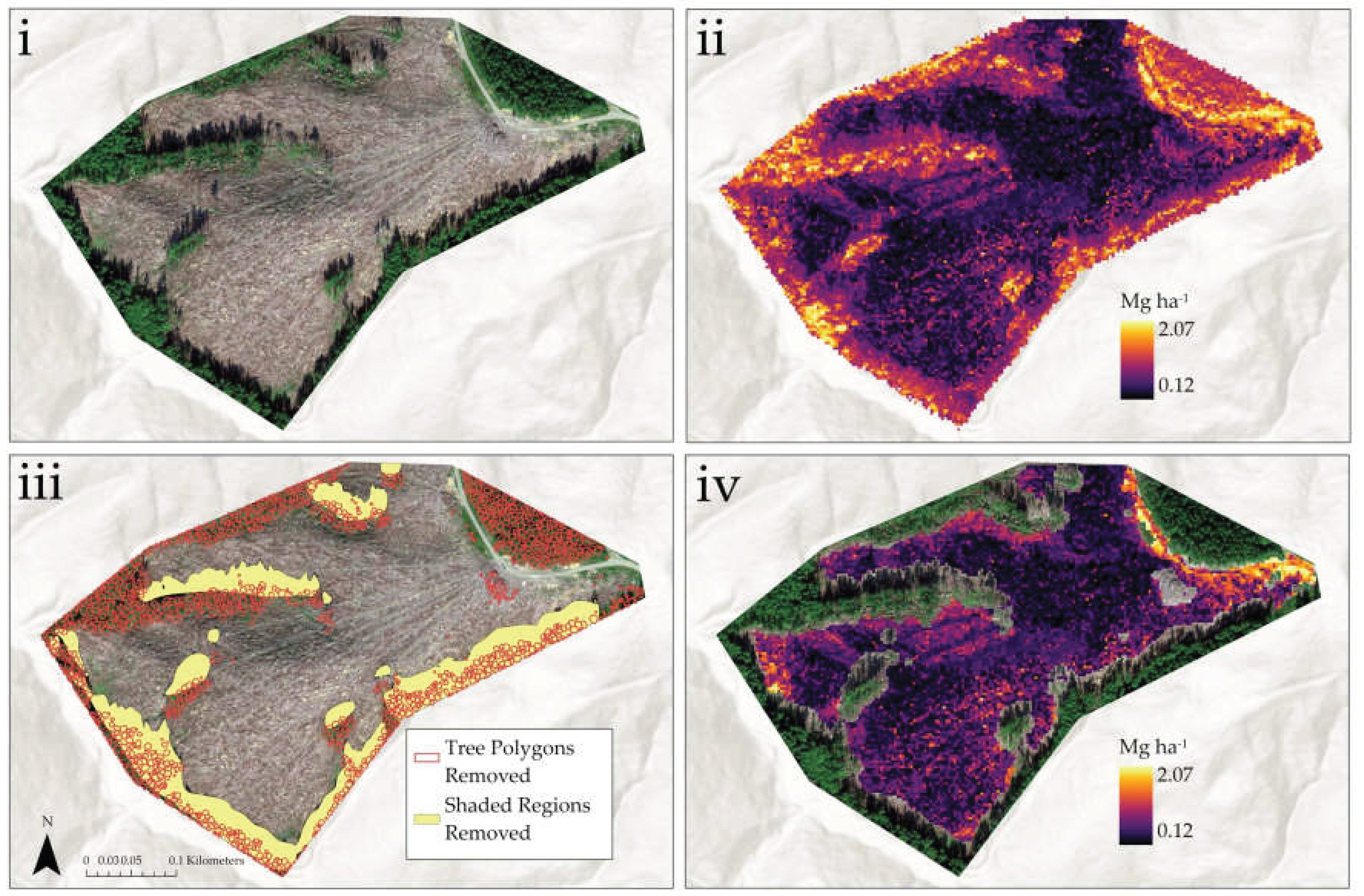
Table 1.
Study site information for the two areas where field and remote sensing data were acquired. For Acquisition A (UAV-LiDAR-Multispectral), field and remote sensing data were both acquired during the summer of 2024. For Acquisition B (UAV-SfM-Multispectral), field and remote sensing data were both acquired during the summer of 2025. .
Table 1.
Study site information for the two areas where field and remote sensing data were acquired. For Acquisition A (UAV-LiDAR-Multispectral), field and remote sensing data were both acquired during the summer of 2024. For Acquisition B (UAV-SfM-Multispectral), field and remote sensing data were both acquired during the summer of 2025. .
| Study Site | Year Harvested |
Year Herbicided |
Year Planted | Hectares Flown for A | # of Ground Plots for A | Hectares Flown for B | # of Ground Plots for B |
|---|---|---|---|---|---|---|---|
| T3 Watershed Experiment |
2024-2025 | NA | NA | 72.5 | 53 | 116.3 | 25 |
| Ethnoforestry field trials | 2018 | 2020 | 2021 | 18.6 | 138 | 98.7 | 158 |
Table 2.
Biomass estimates for stands measured with Acquisition A. These predictions do not include leave-tree areas or areas that were shaded in the imagery, as those were areas where the model had less predictive power. Acquisition B models were not used for prediction because of their poor performance.
Table 2.
Biomass estimates for stands measured with Acquisition A. These predictions do not include leave-tree areas or areas that were shaded in the imagery, as those were areas where the model had less predictive power. Acquisition B models were not used for prediction because of their poor performance.
| Stand Name | Number ha predicted | Total Area (Mg) | Average (Mg ha-1) | Standard Deviation Predicted (Mg ha-1) |
|---|---|---|---|---|
| Variable Density Polyculture | 9.1 | 4.4 | 0.49 | 0.27 |
| Polyculture | 10 | 6.8 | 0.67 | 0.30 |
| Complex Early Seral | 9.1 | 4.3 | 0.48 | 0.20 |
| Ethnoforestry Field Trials North | 6.4 | 8.9 | 1.4 | 0.34 |
| Ethnoforestry Field Trials South | 8.0 | 11 | 1.4 | 0.38 |
Table 3.
The top five most important predictors using relative ranking for the two best models created with Acquisition A (A). Multispectral data were the most important for all tested models. Statistics were calculated for each band within each composite image, so certain bands of composite images scored higher than others. “q” stands for quantile.
Table 3.
The top five most important predictors using relative ranking for the two best models created with Acquisition A (A). Multispectral data were the most important for all tested models. Statistics were calculated for each band within each composite image, so certain bands of composite images scored higher than others. “q” stands for quantile.
| Tested Dataset | Best Model | Most Important Variables | Importance Scores |
|---|---|---|---|
| A: LiDAR and Multispectral | stochastic gradient boosting | Red-edge, band 1, 75th q | 100 |
| Modified Simple Ratio, band 1, 75th q | 68 | ||
| Chlorophyll Index red-edge, band 1, 25th q | 37 | ||
| Near-infrared, band 1, min value | 34 | ||
| Red-edge, band 1, min value | 33 | ||
| A: Multispectral only | stochastic gradient boosting | Red-edge, band 1, 75th q | 100 |
| Modified Simple Ratio, band 1, 75th q | 68 | ||
| Chlorophyll Index red-edge, band 1, 25th q | 42 | ||
| Near-infrared, band 1, min value | 37 | ||
| Red-edge, band 1, min value | 30 |
Disclaimer/Publisher’s Note: The statements, opinions and data contained in all publications are solely those of the individual author(s) and contributor(s) and not of MDPI and/or the editor(s). MDPI and/or the editor(s) disclaim responsibility for any injury to people or property resulting from any ideas, methods, instructions or products referred to in the content. |
© 2026 by the authors. Licensee MDPI, Basel, Switzerland. This article is an open access article distributed under the terms and conditions of the Creative Commons Attribution (CC BY) license (http://creativecommons.org/licenses/by/4.0/).
Copyright: This open access article is published under a Creative Commons CC BY 4.0 license, which permit the free download, distribution, and reuse, provided that the author and preprint are cited in any reuse.


