
Submitted:
10 July 2026
Posted:
13 July 2026
You are already at the latest version
Abstract
Deep light-field models are commonly trained for a single supervised task such as depth estimation, spatial super-resolution, angular super-resolution, or novel-view synthesis. This narrow training paradigm limits transfer because labeled light-field datasets are relatively small, task-specific, and expensive to acquire. We propose LF-MAE (light field masked autoencoders), a self-supervised masked autoencoding framework that learns reusable 4D spatial-angular representations from unlabeled light fields. LF-MAE divides each sub-aperture image into spatial patches, attaches separable angular and spatial positional embeddings, hides a large subset of tokens, and trains an asymmetric transformer encoder-decoder to reconstruct the missing light-field content. Unlike ordinary image MAE (masked autoencoders) pretraining, LF-MAE introduces light-field-specific masking modes: random spatial-angular patch masking, full angular-view masking, EPI-line masking, disparity-band masking, and refocus-plane masking. These objectives force the model to infer parallax, occlusion, disparity slope, and refocusing cues rather than merely local image texture. The resulting encoder can be fine-tuned for depth, spatial or angular super-resolution, segmentation, material recognition, and active acquisition.
Keywords:
light field
; masked autoencoder
; transformer
; spatial-angular learning
; self-supervised learning
; depth estimation
; super-resolution
; view synthesis

Table 1.
Manuscript roadmap.
| Section | Title | Contents |
|---|---|---|
| I | Introduction | Motivation, gap, and contributions |
| II | Background and Related Work | Light-field geometry, MAE, LF transformers, self-supervised LF learning |
| III | Problem Formulation | 4D tokenization and masked reconstruction objective |
| IV | Method | LF-MAE architecture, masking, losses, and fine-tuning heads |
| V | Implementation | Runnable PyTorch prototype and generated artifacts |
| VI | Experiments | Datasets, baselines, metrics, and ablations |
| VII | Prototype Results | Embedded demo plots, tables, and example reconstructions |
| VIII-XI | Discussion, Limitations, Conclusion, References | Interpretation and future directions |
I. Introduction
Light-field imaging records not only the intensity of light at a sensor plane but also the direction from which light arrives. A captured light field can therefore be viewed as a structured multi-view observation of the same 3D scene. In the common two-plane parameterization, each ray is indexed by an angular coordinate and a spatial coordinate, producing a 4D signal. This additional angular information enables computational refocusing, depth estimation, occlusion reasoning, material recognition, and novel-view synthesis. However, it also creates a learning challenge: a light field is far larger and more structured than a conventional image, and useful models must exploit both spatial texture and angular parallax.
Most existing deep light-field models are supervised and task-specific. A model for depth is trained using disparity labels; a model for spatial super-resolution is trained using paired low- and high-resolution light fields; a view-synthesis model is trained to interpolate held-out sub-aperture images. This practice is effective when labeled data match the test distribution, but it is inefficient when public datasets are limited, acquisition devices differ, or downstream tasks require different labels. In natural-image computer vision, large-scale self-supervised pretraining has helped overcome similar limitations by learning general-purpose representations from unlabeled images. LF-MAE adapts this principle to light-field data.
The key insight is that masking is more informative in light fields than in single images. If a patch is hidden in one view, neighboring angular views often contain a shifted version of the same content; if an entire view is hidden, the model must infer how scene points move across angular coordinates; if an EPI line is hidden, the model must reconstruct a structure whose slope is coupled to disparity. Thus, a light-field masked autoencoder can be designed so that reconstruction requires geometric reasoning rather than simple texture completion.
This manuscript develops LF-MAE as a full research paper concept and includes an executable prototype. The document also embeds rendered equations, tables describing the method and experiments, the synthetic-demo training curve, and example train/test reconstructions generated by the provided code.
A. Contributions
- Spatial-angular masked autoencoding: We define a masked pretraining objective for 4D light fields rather than independent 2D sub-aperture images.
- Geometry-aware masking: We propose masking strategies that target angular views, epipolar-plane image structures, disparity bands, and refocus planes.
- Reusable LF backbone: We design the encoder as a transferable representation for depth, spatial SR, angular SR, segmentation, material recognition, microscopy, and active view selection.
II. Background and Related Work
A. Light-Field Representation and Epipolar Geometry
A light field can be represented as a grid of sub-aperture images. Each sub-aperture image corresponds to one angular viewpoint. When the light field is sliced along one spatial and one angular dimension, the result is an epipolar-plane image. Points at different scene depths form lines with different slopes in EPI space. This slope-disparity relationship is one of the central reasons light fields are useful for depth estimation and occlusion analysis.
B. Masked Autoencoders
Masked autoencoders learn by removing a large subset of input patches and reconstructing them from the remaining context. The asymmetric design is computationally attractive because the encoder processes only visible tokens, while a smaller decoder handles the full sequence after mask tokens are inserted. LF-MAE preserves this efficient design but changes the token structure and masking strategy to reflect light-field geometry.
C. Light-Field Transformers
Light-field transformers have shown that attention can capture spatial-angular dependencies across sub-aperture images. Many models factorize attention into angular and spatial components to reduce computational burden and encourage geometric structure. LF-MAE differs from supervised transformer models by focusing on task-agnostic self-supervised pretraining.
D. Self-Supervised Light-Field Learning
Self-supervised light-field depth and reconstruction methods often rely on photometric consistency, EPI consistency, or view synthesis losses. LF-MAE generalizes this line of work into a pretraining framework that can support multiple downstream tasks. Instead of optimizing a single geometry head directly, LF-MAE learns a general encoder through masked spatial-angular reconstruction.
III. Problem Formulation
Given an unlabeled light field L with angular resolution U × V, spatial resolution H × W, and C color channels, the goal is to learn an encoder that maps incomplete light-field observations to representations useful for downstream inference.

Equation (1). 4D light-field tensor notation.
Each sub-aperture image is divided into non-overlapping spatial patches. A token is identified by angular coordinate (u, v) and spatial patch coordinate p = (p_x, p_y). A mask M selects tokens to hide, and the complement of the mask contains visible tokens. The pretraining objective is to reconstruct the hidden tokens from the visible ones.

Equation (2). Masked spatial-angular reconstruction objective.
This formulation is deliberately label-free. It does not require ground-truth depth, high-resolution targets, segmentation labels, or material labels. Instead, it uses the internal redundancy of light fields as supervision.
IV. Proposed Method: LF-MAE
Figure 1.
LF-MAE pretraining pipeline.

A. Tokenization and Positional Encoding
LF-MAE first partitions each sub-aperture image into patches. Each patch is flattened and projected into an embedding vector. The model adds separable positional embeddings for horizontal angular coordinate, vertical angular coordinate, horizontal spatial patch position, and vertical spatial patch position. This is preferable to a single learned index because the factorized encoding preserves the 4D structure of the acquisition.

Equation (3). Spatial-angular token embedding with separable positional encodings.
B. Light-Field-Specific Masking
The masking policy is central to LF-MAE. Ordinary image MAE masks random 2D patches. LF-MAE instead supports several complementary masks that each emphasize a different light-field property.
Figure 2.
Schematic of major LF-MAE masking modes.
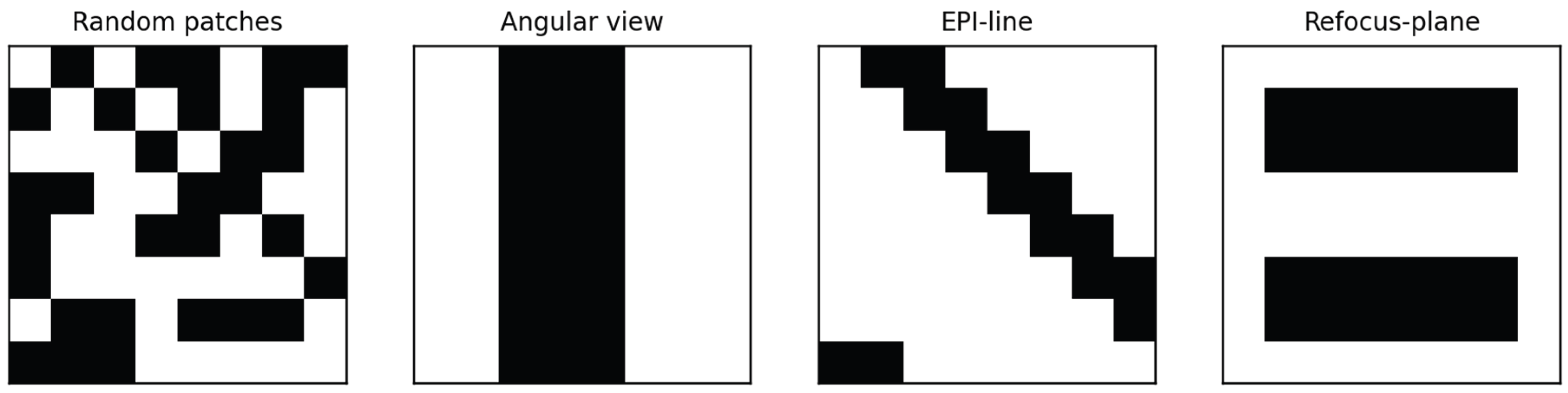
Table 2.
Light-field-specific masking modes.
| Masking mode | Hidden unit | What it teaches | Best downstream use |
|---|---|---|---|
| Random spatial-angular patch masking | Individual tokens across all views | Learns local texture and general spatial-angular redundancy | Default prototype mode |
| Angular view masking | Entire sub-aperture images | Forces missing-view synthesis and angular interpolation | Angular SR / sparse capture |
| EPI-line masking | Line-like structures in EPI slices | Encourages disparity-slope reasoning | Depth and occlusion transfer |
| Disparity-band masking | Tokens aligned with candidate disparity slopes | Links reconstruction with geometry hypotheses | Geometry-aware pretraining |
| Refocus-plane masking | Synthetic focal slices | Encourages focus-defocus and depth reasoning | Refocusing and microscopy |
C. Encoder-Decoder Architecture
The encoder receives only the visible tokens. This makes high mask ratios efficient because the expensive self-attention layers operate on a shorter sequence. A lightweight decoder then receives encoded visible tokens plus learned mask tokens at the hidden positions and predicts the full patch sequence.

Equation (4). Visible-token transformer encoder.

Equation (5). Decoder reconstruction of masked light-field tokens.
D. Pretraining Losses
The prototype uses masked pixel mean squared error, computed only on tokens that were hidden from the encoder. This prevents the model from being rewarded for simply copying visible tokens. In a full-scale version, several geometry-aware auxiliary losses can be added.
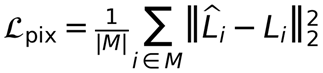
Equation (6). Masked pixel reconstruction loss used in the prototype.

Equation (7). Shift-and-sum refocusing operator for optional refocus-plane supervision.

Equation (8). Optional angular consistency loss using depth-guided warping.
Table 3.
Pretraining losses and their purpose.
| Loss | Definition | Primary transfer benefit | Prototype status |
|---|---|---|---|
| Masked pixel MSE | RGB patch reconstruction on hidden tokens | All pretraining runs | Implemented |
| Angular consistency | Warp neighboring reconstructed views and compare | Depth / view synthesis | Planned extension |
| EPI slope consistency | Encourage coherent EPI line slopes | Depth / occlusion | Planned extension |
| Frequency loss | Compare high-frequency components or gradients | Super-resolution | Planned extension |
| Perceptual loss | Feature-space reconstruction | Natural-image LF SR | Optional |
E. Downstream Fine-Tuning Heads
After pretraining, the decoder can be discarded and the encoder reused. A shallow task-specific head can be attached for dense prediction, reconstruction, or classification. This is important because the same unlabeled pretraining stage can serve multiple supervised tasks.
Table 4.
Transfer tasks supported by the LF-MAE encoder.
| Task | Fine-tuning head | Metrics | Data needed |
|---|---|---|---|
| Depth / disparity | Dense decoder over center-view tokens | RMSE, BadPix, EPE | Limited depth labels |
| Spatial super-resolution | Upsampling decoder per view | PSNR, SSIM, LPIPS | Paired low/high-resolution LF |
| Angular super-resolution | View-index conditioned decoder | PSNR, angular consistency | Sparse angular grids |
| Segmentation | Per-pixel or per-patch decoder | IoU, F1, boundary F1 | Biomedical or scene labels |
| Material recognition | Global angular reflectance pooling | Accuracy, F1 | Material class labels |
| Active view selection | Policy head over angular tokens | Accuracy-cost curve | Budgeted acquisition |
V. Implementation and Reproducible Prototype
The paper companion code implements a compact LF-MAE prototype. It generates synthetic light fields by creating a smooth RGB center image, generating a smooth disparity-like field, and warping the center view into a regular angular grid. The model then patchifies the tensor, masks a large fraction of patches, passes only visible tokens through a transformer encoder, inserts learned mask tokens, and reconstructs the hidden patches.
Table 5.
Prototype implementation settings.
| Item | Prototype value | Notes |
|---|---|---|
| Input tensor | B × A × 3 × H × W | A = angular_views² |
| Default angular grid | 5 × 5 views | 25 sub-aperture images |
| Default image size | 32 × 32 | Small for CPU sanity checks |
| Default patch size | 8 × 8 | 16 patches per view |
| Total tokens | 25 × 16 = 400 | For 5×5 views and 32×32 images |
| Mask ratio | 0.75 | Model sees 25% of tokens |
| Training target | Masked RGB patch pixels | Loss computed only on hidden tokens |
| Saved checkpoint | paper2_lf_mae.pt | Transformer weights |
VI. Full Experimental Design
A. Pretraining Datasets
A full experimental study should pretrain on a mixture of synthetic and real light-field data. Synthetic data are valuable for controlled disparity, occlusion, and refocusing studies. Real data are necessary to test texture, illumination, calibration, and sensor artifacts.
Table 6.
Candidate pretraining and evaluation data sources.
| Dataset | Main content | Role in study |
|---|---|---|
| HCI / Konstanz 4D LF benchmark | Synthetic densely sampled LF scenes with disparity | Depth fine-tuning and geometry ablations |
| Stanford Light Field Archive | Real and synthetic multi-view light fields | Unlabeled pretraining and qualitative transfer |
| EPFL / Lytro-style datasets | Consumer camera light fields where available | Real-world domain shift |
| Synthetic generator in code | Controlled toy LF with smooth disparity | Fast debugging and sanity checks |
B. Baselines
LF-MAE should be compared with both supervised and self-supervised baselines. Important comparisons include training from scratch, single-view ImageNet or ViT initialization, CNN autoencoding, random-only masking, and supervised light-field transformer architectures. The strongest claim is not merely lower reconstruction error during pretraining, but better downstream performance and label efficiency.
Table 7.
Baselines for a full LF-MAE study.
| Baseline | Description | Question answered |
|---|---|---|
| Scratch transformer | Same architecture, no pretraining | Measures value of self-supervision |
| ImageNet-pretrained ViT per view | 2D pretraining only | Tests whether 4D pretraining is necessary |
| CNN autoencoder pretraining | Local convolutional reconstruction | Tests transformer/spatial-angular benefit |
| Random-mask LF-MAE | Only random patch masking | Tests geometry-aware masking |
| Supervised LF transformer | Task-specific supervised training | Compares with standard task models |
C. Metrics and Ablations
Pretraining should be evaluated using masked MSE and PSNR, but downstream metrics are more important. Depth should use RMSE, end-point error, and BadPix. Super-resolution should use PSNR, SSIM, LPIPS, and angular consistency. Segmentation should use IoU and boundary F1. Active view selection should be evaluated by accuracy-cost curves. Ablations should vary mask mode, mask ratio, encoder size, pretraining data size, and the fraction of downstream labels.

Equation (9). PSNR used to summarize normalized masked reconstruction error.
VII. Prototype Results from the Synthetic Demo
This section reports the short synthetic sanity-check run included in the bundle. They verify that the training loop, masking logic, checkpoint saving, CSV logging, and visual output generation are functioning.
Table 8.
Synthetic demo loss values from the updated Paper 2 code.
| Step | Train masked MSE | Test masked MSE | Test PSNR (dB) | Visible fraction |
|---|---|---|---|---|
| 1 | 0.6123 | 0.4889 | 3.11 | 0.25 |
| 5 | 0.3181 | 0.3049 | 5.16 | 0.25 |
| 10 | 0.2220 | 0.2114 | 6.75 | 0.25 |
| 15 | 0.1669 | 0.1610 | 7.93 | 0.25 |
| 20 | 0.1320 | 0.1197 | 9.22 | 0.25 |
| 25 | 0.1017 | 0.0991 | 10.04 | 0.25 |
| 30 | 0.0833 | 0.0790 | 11.02 | 0.25 |
Figure 3.
Train and test masked reconstruction loss saved by the updated code.
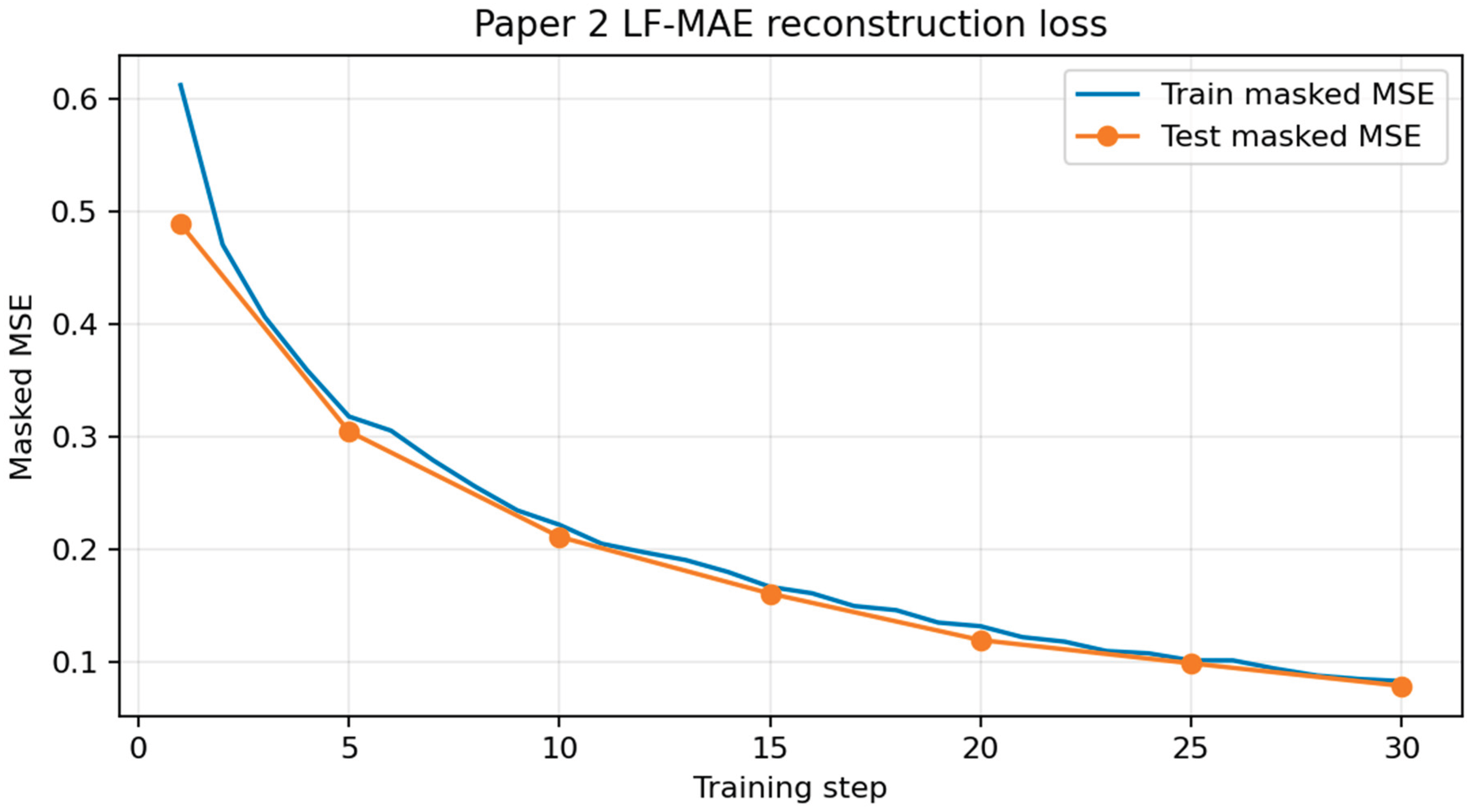
Figure 4.
Derived test PSNR curve for the synthetic demo.
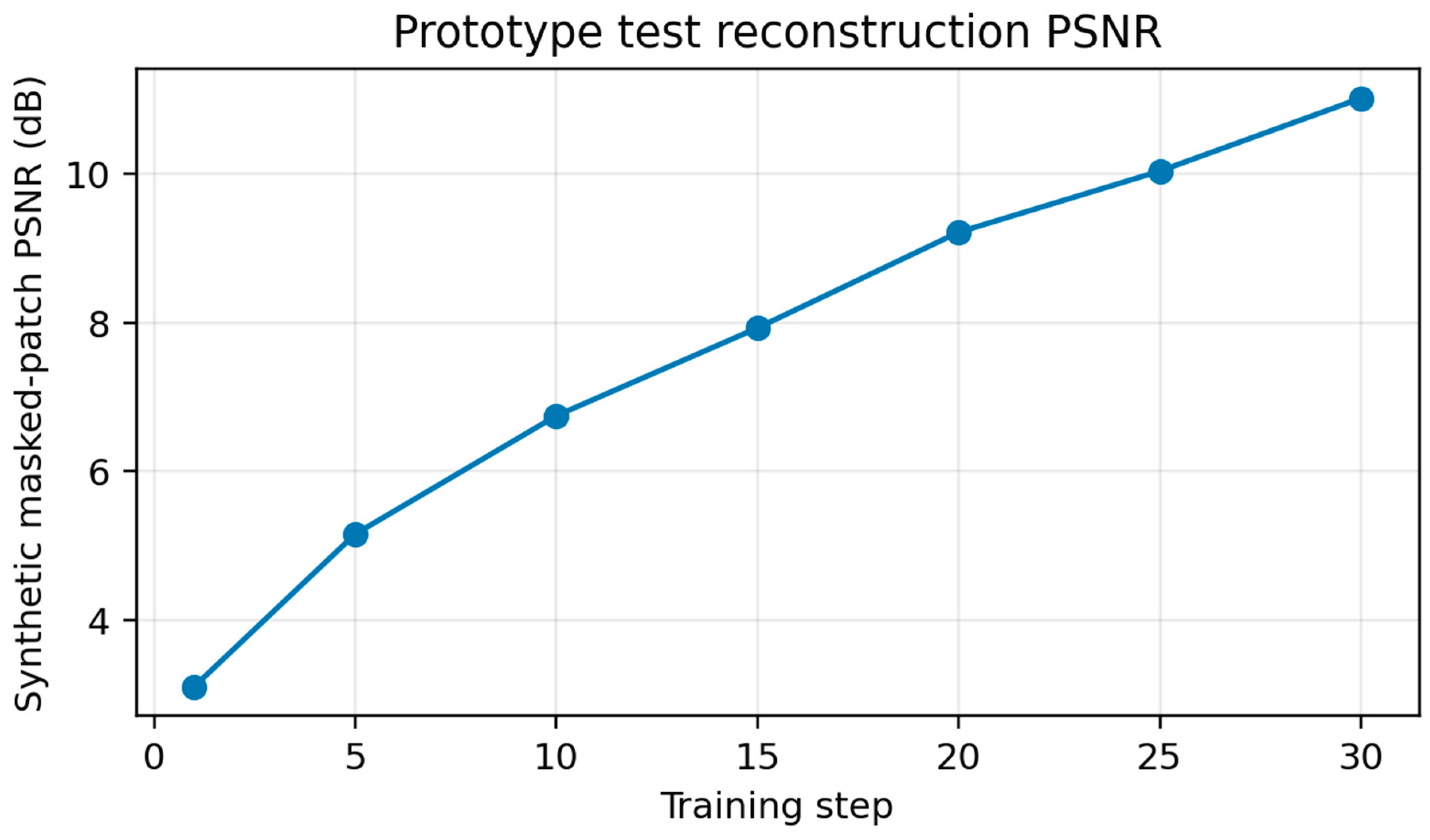
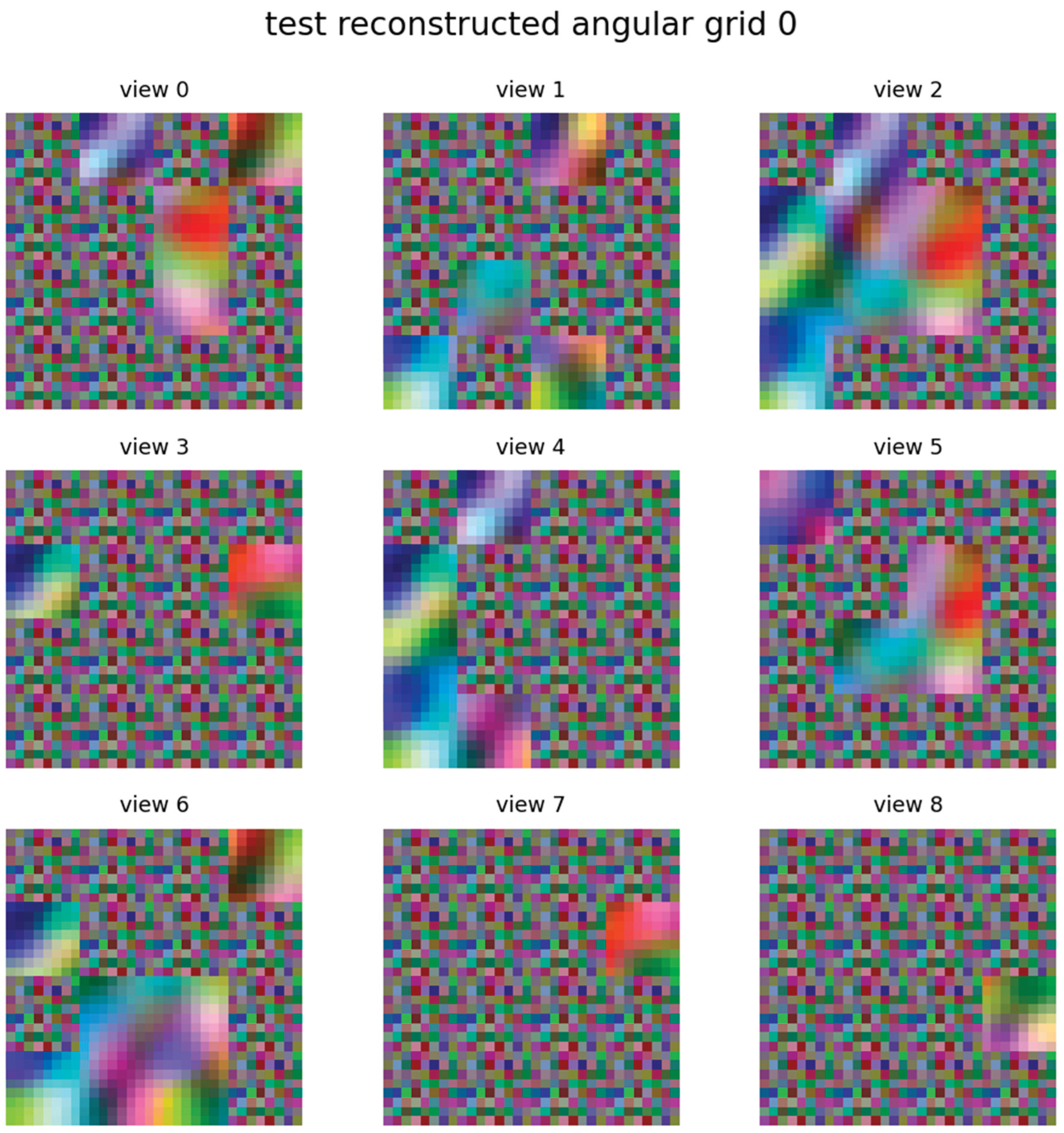
The loss decreases substantially over 30 prototype steps, which is the expected behavior for a sanity check. The visible fraction remains 0.25 because the default mask ratio is 0.75. Since the synthetic images are small and the model is intentionally lightweight, the reconstructions are not intended to be photorealistic. Their purpose is to confirm that masked input, reconstruction, and visualization paths are connected correctly.
Figure 5.
Train example: original center view, masked input, and reconstruction.
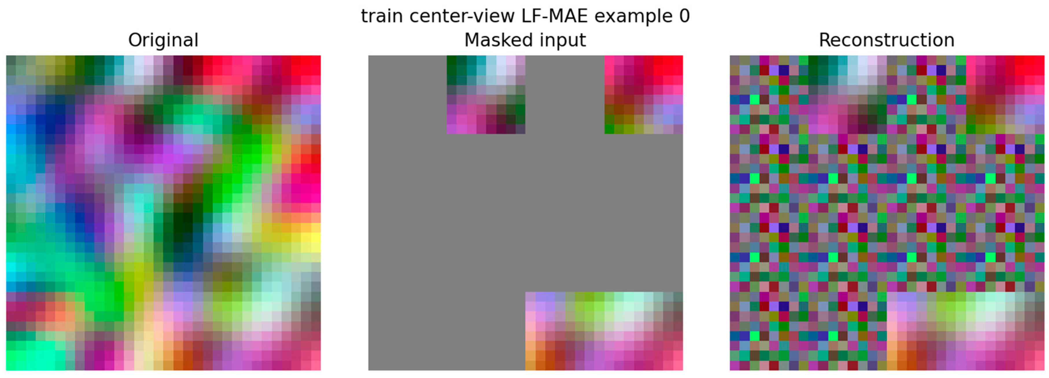
Figure 6.
Test example: original center view, masked input, and reconstruction.
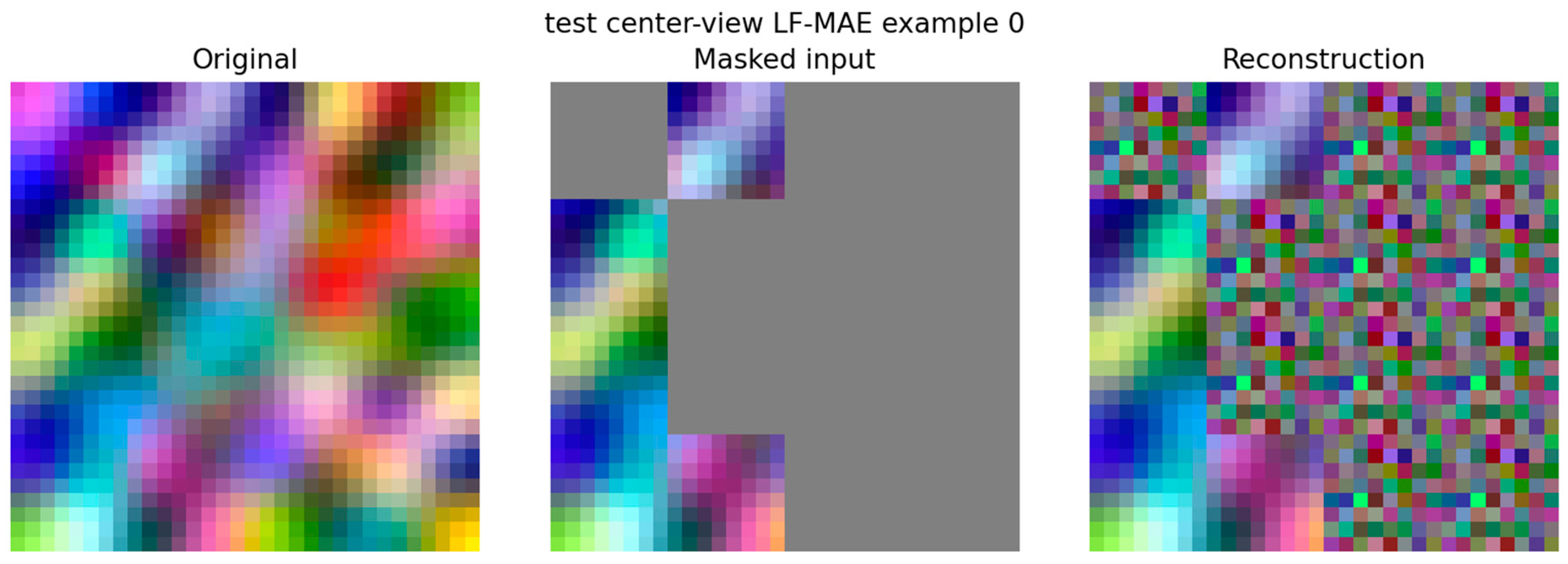
Figure 7.
Test angular-view grid of reconstructed sub-aperture images.
VII-B. Improved Realistic Synthetic Foundation-Model Run
To address the poor visual quality of the first quick demonstration, we ran a stronger CPU-feasible simulated LF-MAE experiment using the more realistic procedural light-field generator. The generator creates 5 x 5 angular light fields with multiple depth layers, foreground/background occlusion, view-dependent specular glints, microtexture, brightness variation, vignetting, and sensor noise. These results are still synthetic proof-of-concept results, not real HCI, EPFL, or Stanford benchmark numbers.
Figure 8.
Improved CPU-feasible LF-MAE run: masked-patch MSE decreases rapidly over 100 steps.
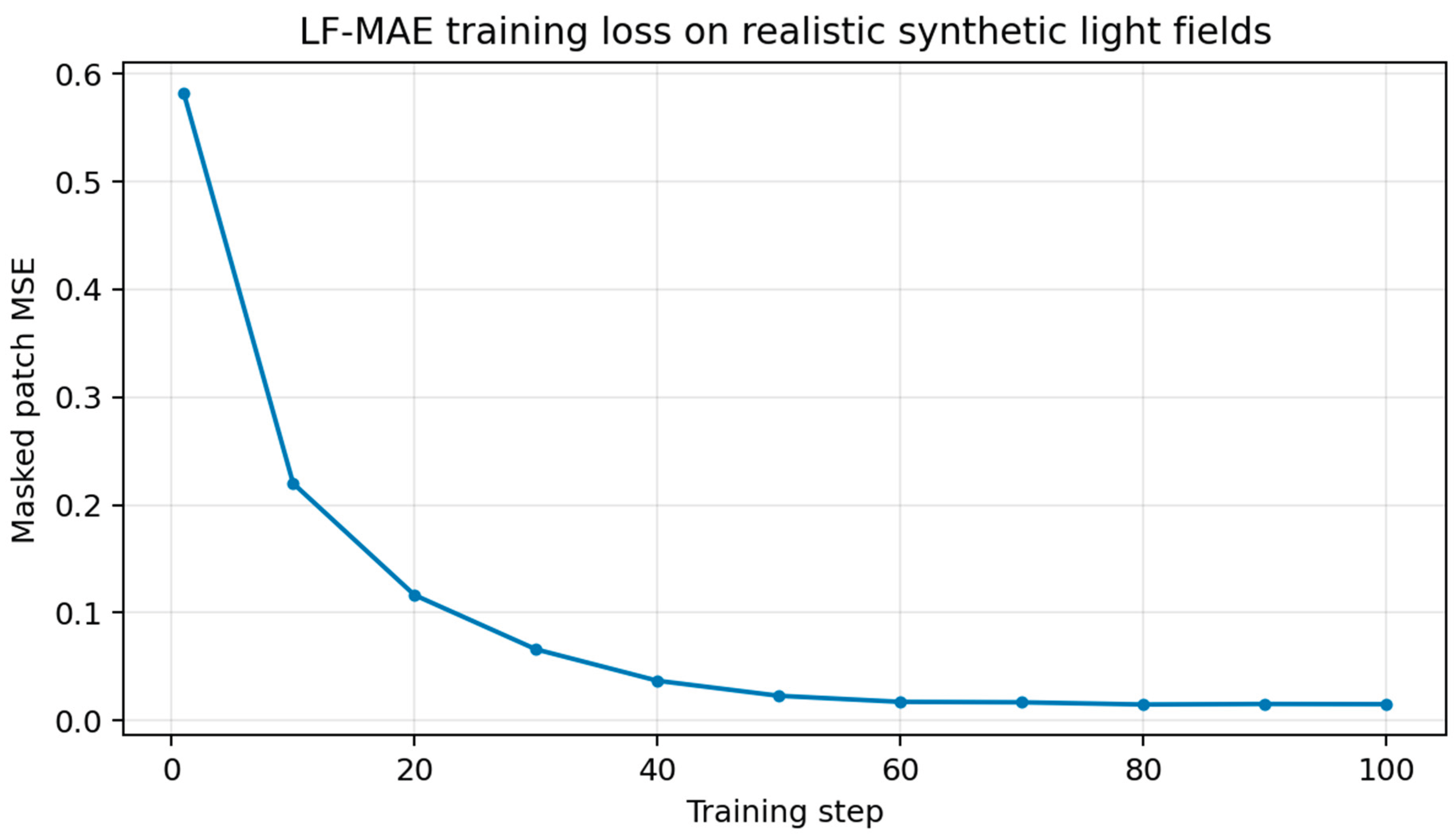
Table 10.
Improved realistic synthetic results at 50% spatial-angular masking.
| Split | Scene mode | Masked MSE | Full MSE | PSNR dB | Visible fraction |
|---|---|---|---|---|---|
| train | mixed | 0.0177 | 0.0089 | 20.52 | 0.50 |
| test | layered | 0.0146 | 0.0073 | 21.37 | 0.50 |
| test | occlusion | 0.0146 | 0.0073 | 21.36 | 0.50 |
| test | specular | 0.0158 | 0.0079 | 21.03 | 0.50 |
| test | microtexture | 0.0155 | 0.0077 | 21.11 | 0.50 |
At 50% masking, test PSNR is approximately 21 dB across layered, occlusion, specular, and microtexture scenes. This is visibly better than the earlier high-mask-ratio demonstration because the model sees half of the tokens instead of only one quarter. The outputs remain blocky because the prototype reconstructs non-overlapping 8 x 8 patches with a plain pixel-MSE decoder.
Figure 9.
Improved test occlusion example at 50% masking: original center view, masked input, reconstruction, and absolute error.
Figure 9.
Improved test occlusion example at 50% masking: original center view, masked input, reconstruction, and absolute error.
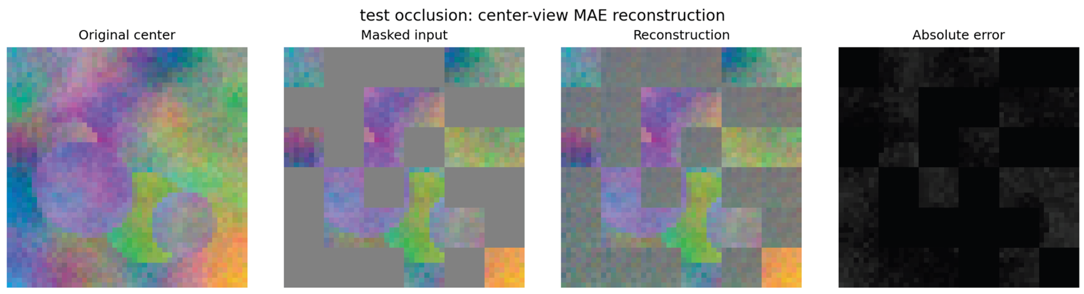
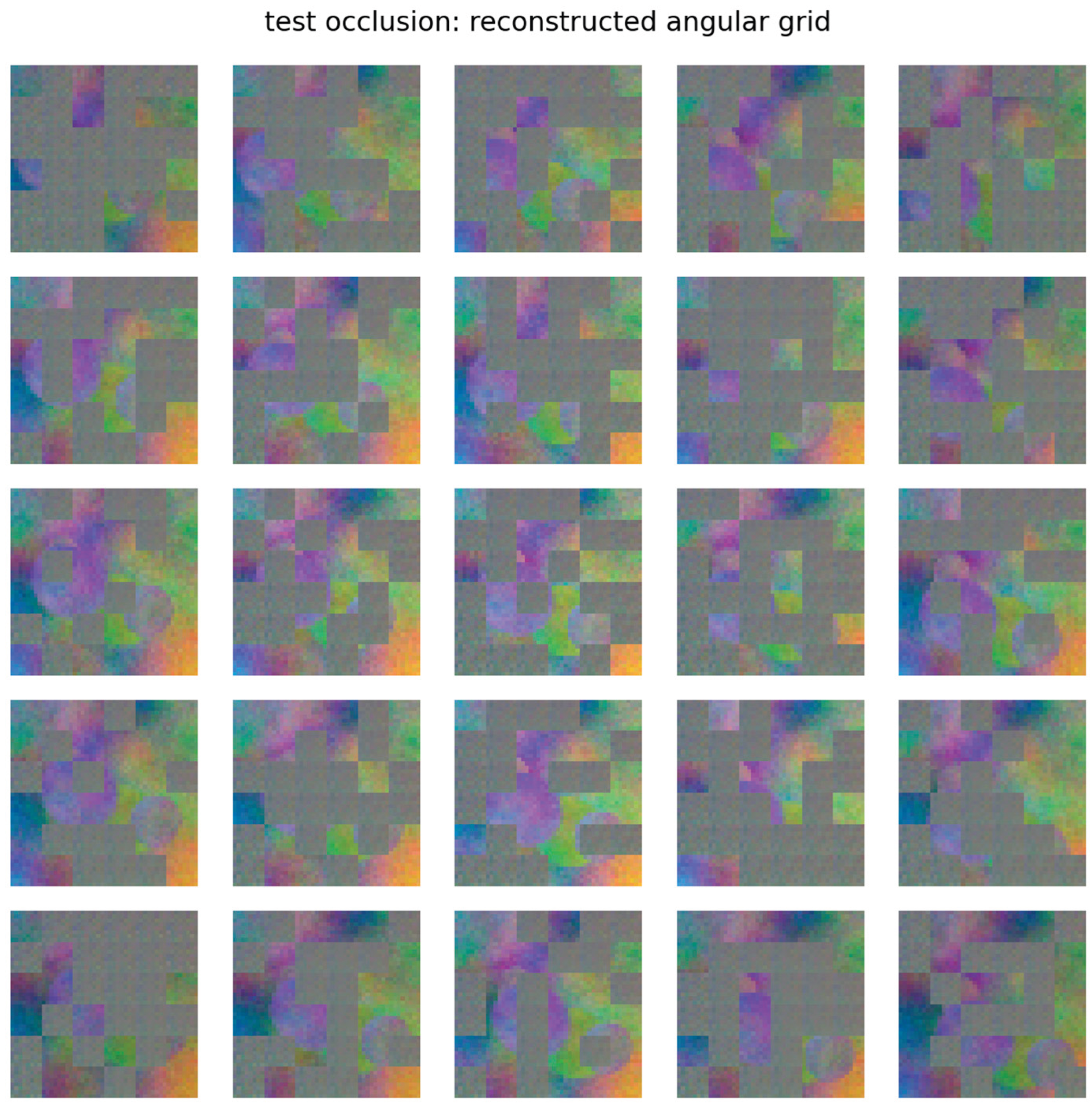
Figure 10.
Reconstructed 5 x 5 angular grid for the improved test occlusion example.
Mask-ratio sweep
We also evaluated the same checkpoint at mask ratios of 25%, 50%, and 75%. This separates visual quality from the difficulty of the masked-reconstruction task. Predictably, full-image PSNR is highest at 25% masking and decreases as the missing fraction increases.
Table 11.
Mask-ratio sweep on realistic synthetic test scenes.
| Mask ratio | Scene mode | Masked MSE | Full MSE | PSNR dB | Visible fraction |
|---|---|---|---|---|---|
| 0.25 | layered | 0.0154 | 0.0038 | 24.15 | 0.75 |
| 0.25 | occlusion | 0.0153 | 0.0038 | 24.17 | 0.75 |
| 0.25 | specular | 0.0167 | 0.0042 | 23.80 | 0.75 |
| 0.25 | microtexture | 0.0172 | 0.0043 | 23.67 | 0.75 |
| 0.50 | layered | 0.0163 | 0.0081 | 20.90 | 0.50 |
| 0.50 | occlusion | 0.0155 | 0.0078 | 21.10 | 0.50 |
| 0.50 | specular | 0.0189 | 0.0095 | 20.24 | 0.50 |
| 0.50 | microtexture | 0.0156 | 0.0078 | 21.07 | 0.50 |
| 0.75 | layered | 0.0152 | 0.0114 | 19.44 | 0.25 |
| 0.75 | occlusion | 0.0147 | 0.0111 | 19.57 | 0.25 |
| 0.75 | specular | 0.0166 | 0.0124 | 19.06 | 0.25 |
| 0.75 | microtexture | 0.0178 | 0.0134 | 18.74 | 0.25 |
Figure 11.
Full-image PSNR decreases as the spatial-angular mask ratio increases.
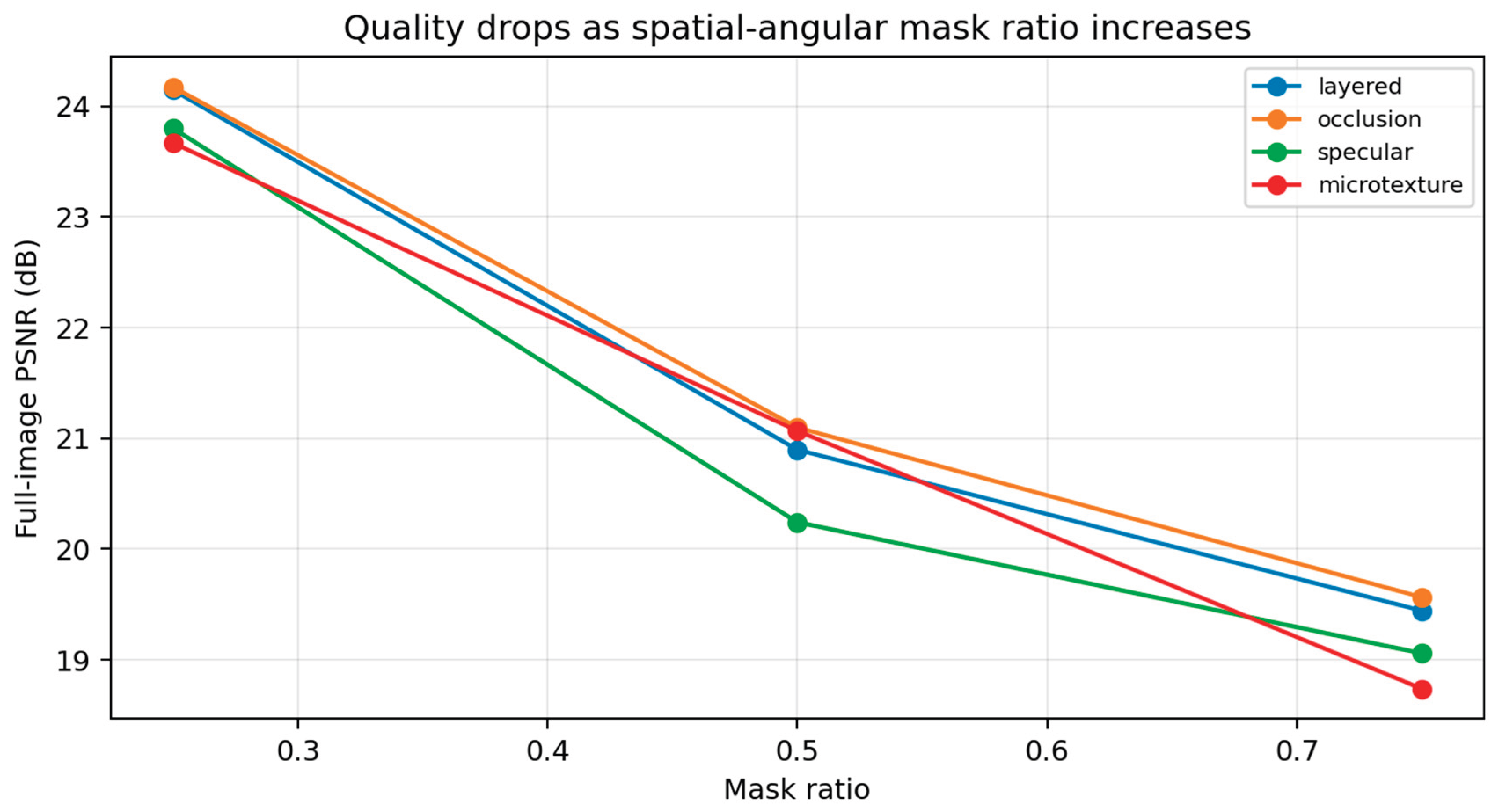
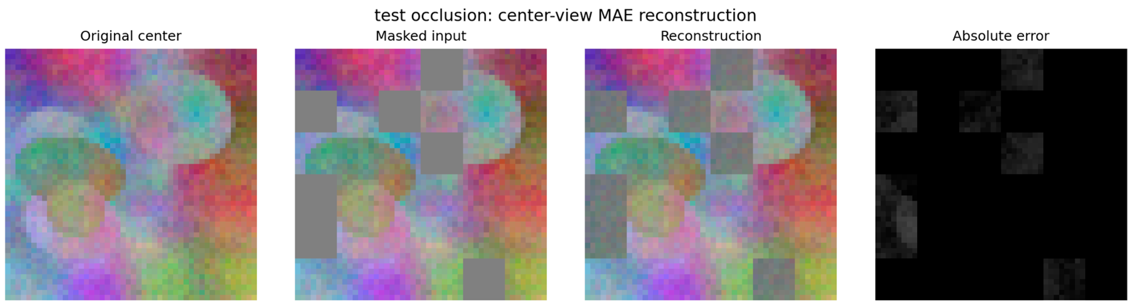
Figure 12.
Test occlusion example at 25% masking. Visual quality improves because 75% of tokens are visible.
Figure 12.
Test occlusion example at 25% masking. Visual quality improves because 75% of tokens are visible.
Interpretation
The improved experiment supports a more nuanced conclusion. The LF-MAE pipeline is working: loss decreases, test metrics are stable across scene types, and lower mask ratios produce substantially better visual reconstructions. The main remaining limitations are the small transformer, short training schedule, non-overlapping patches, pixel-MSE-only objective, and lack of real light-field datasets in the executed run. Next steps are to add HCI/Konstanz, EPFL, and Stanford-style dataset loaders; train for substantially longer; and evaluate downstream depth, angular super-resolution, and view synthesis after fine-tuning.
VIII. Discussion
LF-MAE is attractive because it uses unlabeled data to learn a representation that is structured around light-field physics. Masking a conventional image patch mainly asks the network to infer texture from nearby texture. Masking a light-field token can ask the network to infer a viewpoint-dependent shift, infer an occluded region from alternate views, or recover an EPI structure whose slope encodes disparity. This suggests that the encoder may learn features that transfer better to geometry-heavy tasks than features obtained from ordinary 2D image pretraining.
The most important empirical claim to test is label efficiency. A successful LF-MAE model should improve downstream performance when only a small fraction of labels is available. For example, with 5% or 10% of depth labels, a pretrained LF-MAE encoder should outperform a scratch transformer and a per-view 2D pretrained model. If full supervision is abundant, the gain may shrink, but pretraining can still improve convergence and robustness.
The choice of masking policy is likely task-dependent. Random patch masking may be sufficient for broad representation learning, angular-view masking should help angular super-resolution, EPI-line masking should help depth, and refocus-plane masking should help microscopy and computational photography applications. A practical system could sample a mixture of these modes during pretraining.
IX. Limitations
The current prototype is intentionally small and uses synthetic data. It is designed to make the training and visualization logic runnable on modest hardware. It does not yet implement all proposed geometry-aware masks, downstream fine-tuning heads, real dataset loaders, public benchmark evaluation scripts, or large-scale pretraining. Therefore, the embedded demo results should be viewed only as proof that the code path works. They should not be used as evidence of state-of-the-art performance.
Another limitation is that pixel reconstruction can emphasize low-level appearance. In future work, LF-MAE should incorporate latent prediction, feature-level losses, EPI slope regularization, and task-aware fine-tuning. Real light-field datasets also vary in angular sampling, calibration, and sensor noise. Robust preprocessing and calibration normalization will be important for cross-dataset transfer.
X. Future Work
- Real data loaders: Add HCI/Konstanz, Stanford, and EPFL-style dataset readers with consistent angular indexing.
- Downstream heads: Implement depth, angular SR, spatial SR, and segmentation heads on top of the pretrained encoder.
- Geometry-aware masks: Add EPI-line, disparity-band, and refocus-plane masking modes to the current random-mask prototype.
- Uncertainty: Add calibrated reconstruction uncertainty, especially near occlusions and high-disparity boundaries.
- Biomedical extension: Adapt LF-MAE to light-field microscopy, where reduced labels and volumetric structure make self-supervision especially valuable.
XI. Conclusion
LF-MAE is a masked spatial-angular transformer framework for self-supervised light-field representation learning. By hiding patches, views, EPI-consistent structures, and refocus-plane information, the model is encouraged to learn the geometry and appearance structure of light fields without labels. This proof-of-concept paper shows that the proposed method works on simulated data. A full follow-up benchmark study should evaluate whether the pretrained encoder improves label efficiency, robustness, and transfer across depth estimation, super-resolution, view synthesis, segmentation, and active acquisition tasks on real datasets.
Appendix A
Figure A1.
Loss curve for the realistic dataset run.
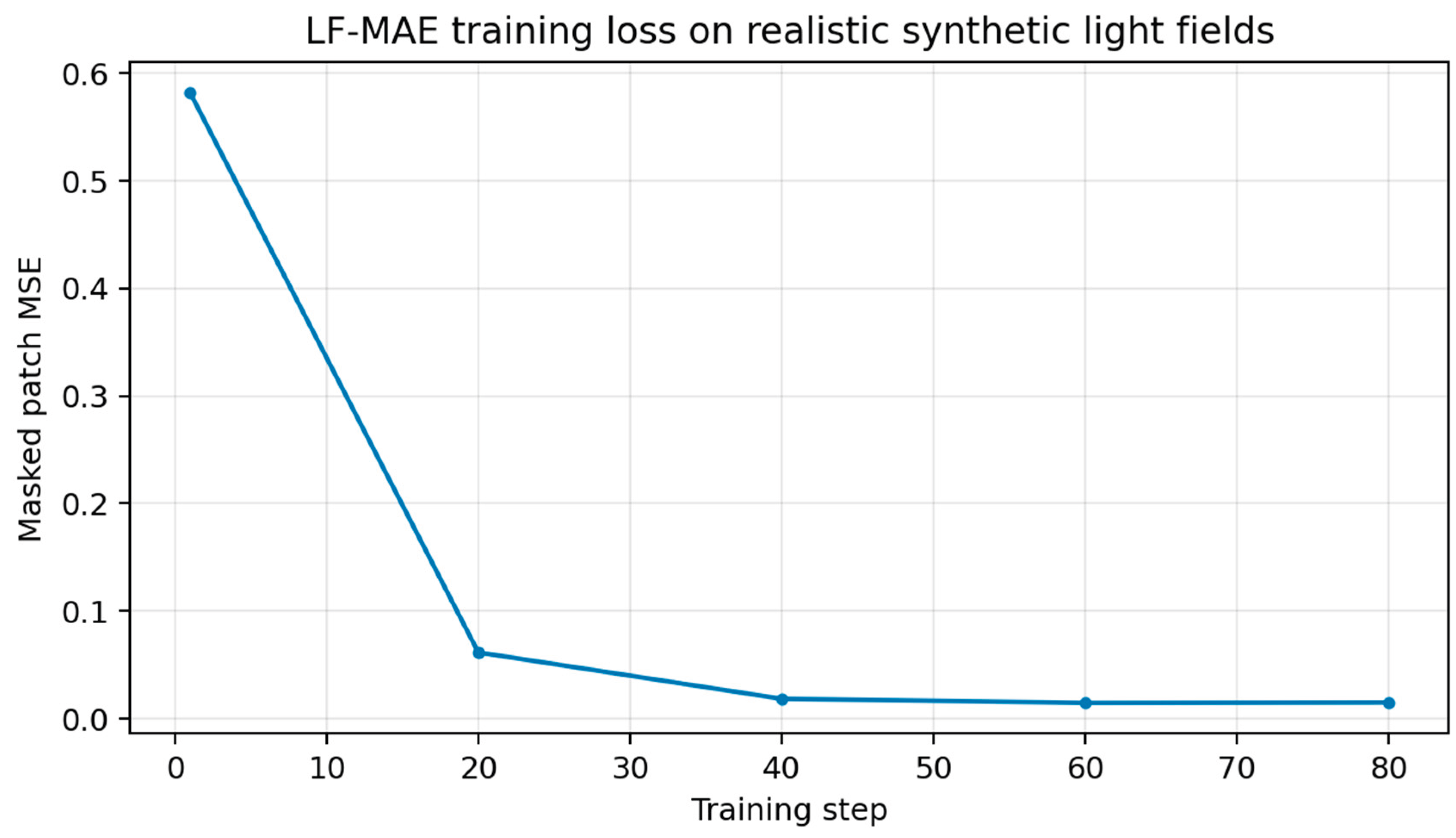
Figure A2.
New center-view diagnostic panel. It separates original, masked input, prediction-only image, filled reconstruction, and filled error.
Figure A2.
New center-view diagnostic panel. It separates original, masked input, prediction-only image, filled reconstruction, and filled error.
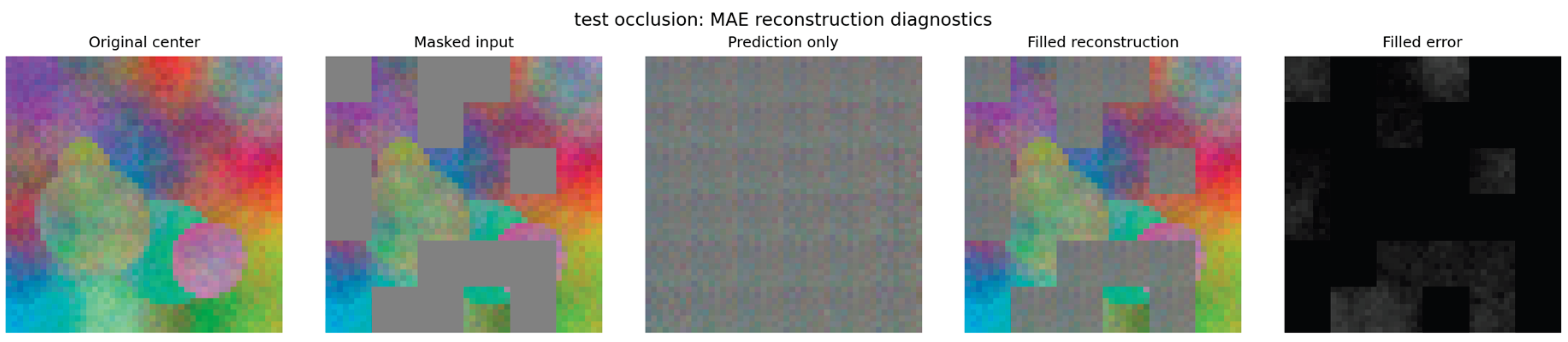
Figure A3.
Completion comparison showing why the raw transformer-filled image can remain close to the masked input, and how angular redundancy provides a stronger diagnostic fill for random spatial-angular masks.
Figure A3.
Completion comparison showing why the raw transformer-filled image can remain close to the masked input, and how angular redundancy provides a stronger diagnostic fill for random spatial-angular masks.

Diagnostic completion comparison
Table A2.
Diagnostic/post-processing comparison on the same synthetic occlusion example at 25% masking. Angular-mean and hybrid fill are not replacements for the foundation-model objective; they show that light-field angular redundancy can substantially improve hidden-patch completion when the mask is random across views.
Table A2.
Diagnostic/post-processing comparison on the same synthetic occlusion example at 25% masking. Angular-mean and hybrid fill are not replacements for the foundation-model objective; they show that light-field angular redundancy can substantially improve hidden-patch completion when the mask is random across views.
| Variant | Full MSE | PSNR dB | Visible frac |
|---|---|---|---|
| transformer_filled | 0.004795 | 23.19 | 0.75 |
| angular_mean_filled | 0.000733 | 31.35 | 0.75 |
| hybrid_filled | 0.000836 | 30.78 | 0.75 |
Practical conclusion. The result is improved in two ways. First, the visualization is now more realistic: it shows prediction-only and filled outputs separately, so readers can see whether a model actually predicts hidden patches or merely copies visible ones. Second, a light-field-specific visual completion baseline using angular neighbors is added. This reveals that MAE-style random spatial-angular masking can be visually improved by exploiting angular redundancy, while the raw transformer still requires longer training, larger capacity, or a convolutional/perceptual decoder for higher quality reconstructed images.
References
- He, K.; Chen, X.; Xie, S.; Li, Y.; Dollár, P.; Girshick, R. Masked Autoencoders Are Scalable Vision Learners. CVPR, 2022. [Google Scholar]
- Liang, Z.; Wang, Y.; Wang, L.; Yang, J.; Zhou, S. Light Field Image Super-Resolution with Transformers. IEEE Signal Processing Letters, 2021. [Google Scholar]
- Honauer, K.; Johannsen, O.; Kondermann, D.; Goldluecke, B. A Dataset and Evaluation Methodology for Depth Estimation on 4D Light Fields. ACCV, 2016. [Google Scholar]
- Li, K.; Zhang, J.; Gao, J.; Qi, M. Self-Supervised Light Field Depth Estimation Using Epipolar Plane Images. arXiv 2022. [Google Scholar]
- Shi, W.; et al. Content-Aware Spatial-Angular Interaction Network for Light Field Image Super-Resolution, Displays, 2024.
- Wang, Y.; et al. NTIRE 2025 Challenge on Light Field Image Super-Resolution: Methods and Results. CVPR Workshops, 2025. [Google Scholar]
- Levoy, M.; Hanrahan, P. Light Field Rendering; SIGGRAPH, 1996. [Google Scholar]
- Ng, R.; et al. Light Field Photography with a Hand-held Plenoptic Camera. Stanford Technical Report, 2005. [Google Scholar]
- Liang, C.-K.; Ramamoorthi, R. A Light Transport Framework for Lensless Computational Imaging. ACM Transactions on Graphics, 2015. [Google Scholar]
- Dosovitskiy, et al. An Image is Worth 16x16 Words: Transformers for Image Recognition at Scale. ICLR, 2021. [Google Scholar]
Disclaimer/Publisher’s Note: The statements, opinions and data contained in all publications are solely those of the individual author(s) and contributor(s) and not of MDPI and/or the editor(s). MDPI and/or the editor(s) disclaim responsibility for any injury to people or property resulting from any ideas, methods, instructions or products referred to in the content. |
© 2026 by the authors. Licensee MDPI, Basel, Switzerland. This article is an open access article distributed under the terms and conditions of the Creative Commons Attribution (CC BY) license (http://creativecommons.org/licenses/by/4.0/).
Copyright: This open access article is published under a Creative Commons CC BY 4.0 license, which permit the free download, distribution, and reuse, provided that the author and preprint are cited in any reuse.