Quaternions as Quantization: The 44-Vector Lattice, the Discrete–Continuous Bridge, and the Geometric Origin of Quantum Non-Commutativity

1. Introduction: The Quantization Problem

1.1. What We Still Don’T Understand

In the standard narrative, quantum mechanics was born in 1925–1926 when Heisenberg, Born, Jordan, Schrödinger, and Dirac discovered that physical observables must be represented by non-commuting operators. The canonical quantization prescription

$${\{A,B\}}_{\mathrm{PB}}⟶{\displaystyle \frac{1}{i\hslash }}[\widehat{A},\widehat{B}],$$

(1)

replacing Poisson brackets with commutators, is taught in every quantum mechanics textbook as a postulate—a rule that works but has no deeper explanation.

A century later, the situation is philosophically unsatisfying. Why must observables fail to commute? Why does nature abhor the classical limit of commuting operators? The question is usually dismissed with “that’s just how quantum mechanics works”—but this is a description, not an explanation. The quantization procedure remains the deepest unexplained axiom of modern physics.

1.2. The Quaternion Hypothesis

This paper proposes that the answer has been known since 1843. On October 16 of that year, William Rowan Hamilton carved the fundamental formula

$${\mathbf{i}}^2={\mathbf{j}}^2={\mathbf{k}}^2=\mathbf{i}\mathbf{j}\mathbf{k}=-1$$

(2)

into the stone of Brougham Bridge in Dublin [1]. This equation defines the quaternion algebra $\mathbb{H}$, the first non-commutative algebraic structure in the history of mathematics. Hamilton himself recognized its profundity, spending the remaining 22 years of his life developing quaternion analysis as the “natural language of physics.”

Hamilton failed—not because quaternions were wrong, but because the physical theory that required them (quantum mechanics) would not be discovered for another 82 years. When Heisenberg [3] and Born–Jordan [4] introduced matrix mechanics in 1925, they reinvented non-commutativity as a physical principle, unaware that Hamilton’s quaternions had already encoded it as a geometric fact:

$$\mathbf{i}\mathbf{j}-\mathbf{j}\mathbf{i}=2\mathbf{k},\mathbf{j}\mathbf{k}-\mathbf{k}\mathbf{j}=2\mathbf{i},\mathbf{k}\mathbf{i}-\mathbf{i}\mathbf{k}=2\mathbf{j}.$$

(3)

These are precisely the commutation relations of the Pauli matrices (up to the factor $2i$). The Pauli matrices ${\sigma }_x,{\sigma }_y,{\sigma }_z$ are nothing but the quaternion basis $\mathbf{i},\mathbf{j},\mathbf{k}$ in the fundamental 2-dimensional complex representation of $\mathrm{SU}\left(2\right)$:

$${\sigma }_x\sim i\mathbf{i},{\sigma }_y\sim i\mathbf{j},{\sigma }_z\sim i\mathbf{k}.$$

(4)

1.3. This Paper

We argue that quaternions are not merely a “computational tool” or a “convenient representation” of quantum mechanics—their non-commutativity is the geometric origin of quantum non-commutativity in 3-dimensional space. We develop this argument through three interconnected results:

1.

Discrete lattice = quaternion orbit. The 44-vector ${\mathbb{Z}}_3$-triality vacuum lattice—a zero-parameter discrete structure reproducing the Standard Model mass hierarchy, mixing angles, and fine-structure constant [7,8,9,10]—is proved to be the exact orbit closure of the quaternion basis under ${\mathbb{Z}}_3\subset \mathrm{SU}\left(2\right)$ (Theorem 3.1). The three closure operations $T,\Delta ,\kappa$ are unified as conjugations by a single $q_T\in \mathrm{SU}\left(2\right)$ (Proposition 3.1). The proof proceeds by decomposing ${\mathbb{R}}^3\cong \mathrm{im}\left(\mathbb{H}\right)$ into irreducible ${\mathbb{Z}}_3$- representations $V_0\oplus V_1$, establishing the $A_2$ hexagonal root lattice in $V_1$, and enumerating the orbit closure to give $|L_{44}|=36+3+5=44$. The lattice size factorizes as $|L_{44}|={dim}_{\mathbb{R}}\left(\mathbb{H}\right)\times dim{\mathfrak{g}}_0^{\mathrm{eff}}=4\times 11$, a structural identity rather than a coincidence.

2.

Discrete–continuous bridge. Quaternion conjugation $v\mapsto qv{q}^{-1}$ by unit quaternions $q\in \mathrm{SU}\left(2\right)$ provides the natural bridge between the discrete 44-vector lattice and continuous $\mathrm{SU}\left(2\right)$ gauge theory. The ${\mathbb{Z}}_3$ rotation is the restriction of $\mathrm{SU}\left(2\right)$ to its order-3 subgroup; the cross product is one-half the quaternion commutator. The continuum limit is guaranteed by the invariance of the $A_2$ root lattice closure under the full $\mathrm{SU}\left(2\right)$ adjoint action (Theorem 4.1).

3.

Quaternions as the geometry of non-commutativity. The fundamental non-commutative structures of quantum mechanics—the Pauli algebra, the Dirac $\gamma$-matrix algebra, the spin-statistics connection, and the canonical commutator $[\widehat{x},\widehat{p}]=i\hslash$—are traced, at varying levels of mathematical rigor, to the same geometric source: the non-commutativity of quaternion multiplication. We distinguish between results that are strict mathematical facts (Pauli = quaternion), those that follow from structural inheritance (Dirac algebra), and those that are geometric interpretations supported by the framework (canonical quantization). Quantization, in this picture, is not an imposed procedure but a reflection of the non-commutative geometry of space.

2. Quaternions: The Unique Non-Commutative Geometry of 3D Space

2.1. The Algebra

The quaternion algebra $\mathbb{H}$ is the 4-dimensional real algebra with basis $\{1,\mathbf{i},\mathbf{j},\mathbf{k}\}$ satisfying (2). The multiplication is non-commutative: $\mathbf{i}\mathbf{j}=-\mathbf{j}\mathbf{i}=\mathbf{k}$.

The pure imaginary quaternions $\mathrm{im}\left(\mathbb{H}\right)={\mathrm{span}}_{\mathbb{R}}\{\mathbf{i},\mathbf{j},\mathbf{k}\}$ form a 3D real vector space. For $v,w\in \mathrm{im}\left(\mathbb{H}\right)$, the product decomposes as

$$vw=-v·w+v\times w,$$

(5)

where · is the Euclidean dot product and × is the cross product on the component coefficients. The commutator gives the cross product:

$${[v,w]}_{\mathbb{H}}\equiv vw-wv=2(v\times w).$$

(6)

2.2. Frobenius Uniqueness: Why 3 Dimensions Are Forced

Theorem (Frobenius 1877).There are exactly three finite-dimensional associative division algebras over $\mathbb{R}$: the reals $\mathbb{R}$, the complex numbers $\mathbb{C}$, and the quaternions $\mathbb{H}$. [2]

Among these, $\mathbb{H}$ is the unique non-commutative choice. Its pure imaginary subspace has dimension 3—not by accident, but by algebraic necessity. The “three dimensions of space” are the three imaginary quaternion axes. There is no alternative.

This is not a philosophical claim. If space had 4 or 5 dimensions, there would be no quaternion algebra to describe it—and by extension, no non-commutative geometry, no spin-$\frac{1}{2}$ representations, and no quantum mechanics as we know it.

2.3. Why Hamilton Failed and Heisenberg Succeeded

Hamilton believed quaternions were the “natural language” for all of physics. He spent decades attempting to reformulate Newtonian mechanics in quaternion form. He failed because classical mechanics is commutative: forces add, positions multiply, and Poisson brackets are antisymmetric but not fundamentally non-commutative. Quaternions were the solution to a problem that hadn’t been discovered yet.

Heisenberg’s 1925 insight was that physical observables do fail to commute: measuring position then momentum gives a different answer than measuring momentum then position. The mathematical structure he needed— non-commutative multiplication with a geometric interpretation—was exactly what Hamilton had discovered 82 years earlier. Heisenberg did not use quaternions explicitly (he used infinite matrices), but the algebraic core of his discovery was Hamilton’s.

3. The 44-Vector Lattice as the Quaternion Orbit Closure

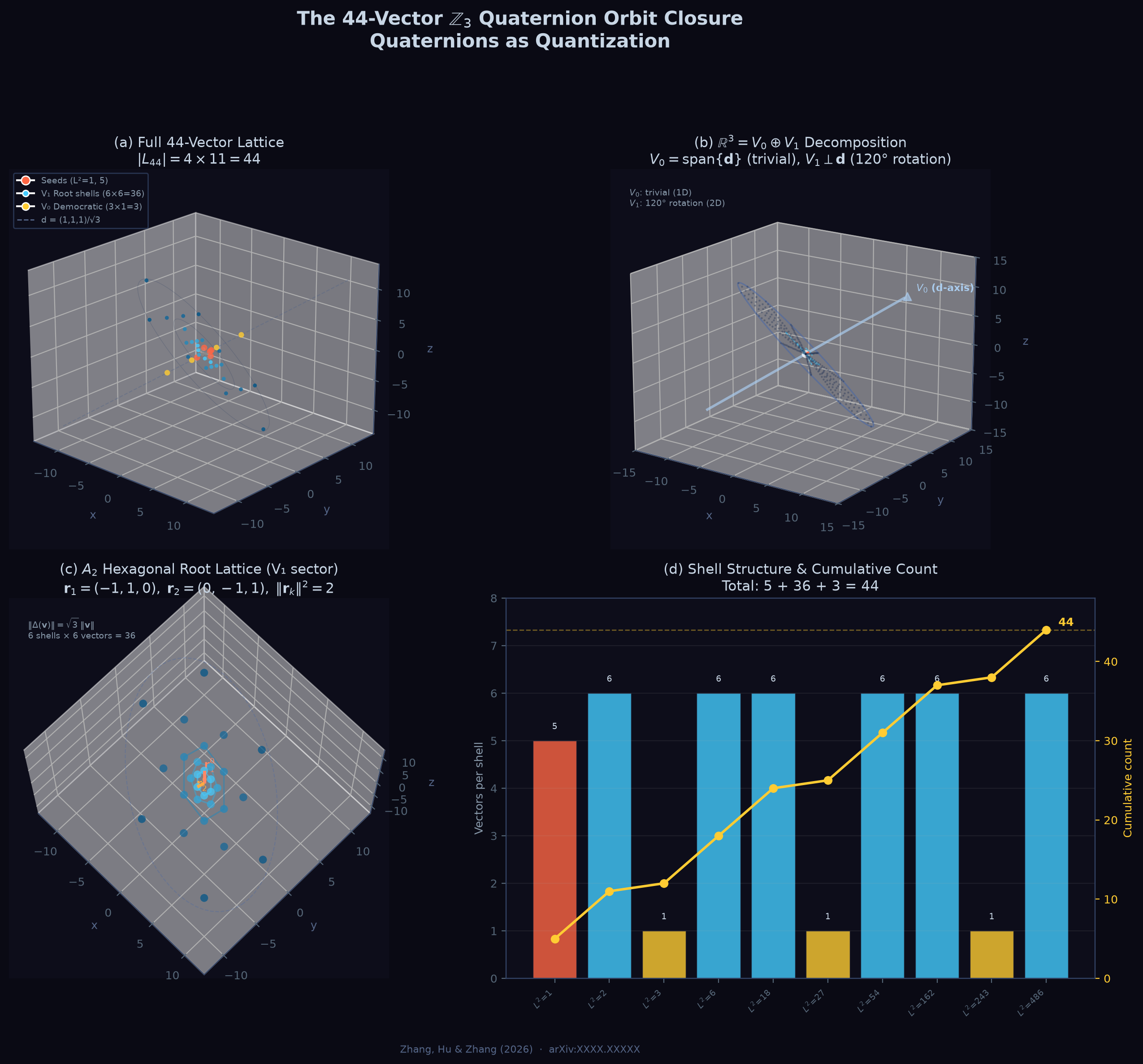
In this section we prove that the 44-vector ${\mathbb{Z}}_3$-triality vacuum lattice $L_{44}$ is exactly the orbit closure of the quaternion basis under the ${\mathbb{Z}}_3\subset \mathrm{SU}\left(2\right)$ subgroup generated by $q_T=\frac{1}{2}(1+\mathbf{i}+\mathbf{j}+\mathbf{k})$. The proof proceeds through: (i) unifying the three ${\mathbb{Z}}_3$ operations under $q_T$, (ii) decomposing ${\mathbb{R}}^3\cong \mathrm{im}\left(\mathbb{H}\right)$ into irreducible ${\mathbb{Z}}_3$- representations, (iii) classifying the $A_2$ root lattice in the rotational plane and the democratic axis, and (iv) enumerating the orbit closure to obtain $|L_{44}|=44$.

3.1. ${\mathbb{Z}}_3$ Closure Unified by Quaternion Conjugation

Definition 1 

(Seed set and closure operators). The ${\mathbb{Z}}_3$-triality vacuum lattice $L_{44}$ is generated from the seed set

$$S=\{{\mathbf{e}}_1,{\mathbf{e}}_2,{\mathbf{e}}_3,\mathbf{d},-\mathbf{d}\},{\mathbf{e}}_1=(1,0,0),{\mathbf{e}}_2=(0,1,0),{\mathbf{e}}_3=(0,0,1),\mathbf{d}=\frac{1}{\sqrt{3}}(1,1,1),$$

(7)

under iterative application of the operators

$$\begin{array}{cc}\hfill T(x,y,z)& =(z,x,y),\hfill \end{array}$$

(8)

$$\begin{array}{cc}\hfill \Delta \left(\mathbf{v}\right)& =T\left(\mathbf{v}\right)-\mathbf{v},\hfill \end{array}$$

(9)

$$\begin{array}{cc}\hfill \kappa \left(\mathbf{v}\right)& =\left\{\begin{array}{cc}{\displaystyle \frac{\mathbf{v}\times T\left(\mathbf{v}\right)}{\parallel \mathbf{v}\times T\left(\mathbf{v}\right)\parallel }},\hfill & \parallel \mathbf{v}\times T\left(\mathbf{v}\right)\parallel >0,\hfill \\ \mathrm{undefined},\hfill & \mathrm{otherwise}.\hfill \end{array}\right.\hfill \end{array}$$

(10)

The orbit closure is the set of all vectors reachable from S by finitely many compositions of $\{T,\Delta ,\kappa \}$ (where defined), taking the first 44 vectors ranked by descending norm.

Proposition 1 

(Quaternion unification of ${\mathbb{Z}}_3$ closure). Under the identification ${\mathbb{R}}^3\cong \mathrm{im}\left(\mathbb{H}\right)$, the three ${\mathbb{Z}}_3$ closure operators are simultaneous consequences of conjugation by a single unit quaternion

$$q_T=\frac{1}{2}(1+\mathbf{i}+\mathbf{j}+\mathbf{k})\in \mathrm{SU}\left(2\right).$$

(11)

Specifically, for any $\mathbf{v}\in {\mathbb{R}}^3\cong \mathrm{im}\left(\mathbb{H}\right)$:

$$\begin{array}{cc}\hfill T\left(\mathbf{v}\right)& =q_T\mathbf{v}{q}_T^{-1}=\mathrm{Ad}\left(q_T\right)\left(\mathbf{v}\right),\hfill \end{array}$$

(12)

$$\begin{array}{cc}\hfill \Delta \left(\mathbf{v}\right)& =\mathrm{Ad}\left(q_T\right)\left(\mathbf{v}\right)-\mathbf{v},\hfill \end{array}$$

(13)

$$\begin{array}{cc}\hfill \kappa \left(\mathbf{v}\right)& ={\displaystyle \frac{1}{2\parallel \mathbf{v}\times T\left(\mathbf{v}\right)\parallel }}{[\mathbf{v},\mathrm{Ad}\left(q_T\right)\left(\mathbf{v}\right)]}_{\mathbb{H}}.\hfill \end{array}$$

(14)

Proof. 

$q_T$ is a unit quaternion: $\parallel q_T{\parallel }^2=\frac{1}{4}(1^2+1^2+1^2+1^2)=1$. Its adjoint action on pure imaginary quaternions is a ${120}^{\circ }$ rotation about the axis $\mathbf{d}={\displaystyle \frac{1}{\sqrt{3}}}(1,1,1)$. Direct computation: for $\mathbf{v}=(x,y,z)\in \mathrm{im}\left(\mathbb{H}\right)$,

$$\begin{array}{cc}\hfill \mathrm{Ad}\left(q_T\right)\left(\mathbf{v}\right)& =q_T(0+xi+yj+zk)q_T^{-1}\hfill \\ \hfill & =\frac{1}{2}(1+i+j+k)(xi+yj+zk)\frac{1}{2}(1-i-j-k)\hfill \\ \hfill & =(0+yi+zj+xk)⟷(y,z,x)=T\left(\mathbf{v}\right).\hfill \end{array}$$

(15)

Equation (13) follows immediately from (12). Equation (6) follows from (12) and the identity ${[v,w]}_{\mathbb{H}}=2(v\times w)$ for $v,w\in \mathrm{im}\left(\mathbb{H}\right)$ (Equation 6), with the normalization factor. □

The significance of Proposition 1 cannot be overstated: the three “independent” ${\mathbb{Z}}_3$ operations that generate the 44-vector lattice are not three choices—they are the rotation, difference, and commutator of a single algebraic generator $q_T$. The lattice is therefore not an ad hoc construction but the necessary orbit structure of the unique non-commutative normed division algebra in 3 dimensions, restricted to its order-3 subgroup.

3.2. Decomposition of ${\mathbb{R}}^3$ Under ${\mathbb{Z}}_3$

Proposition 2 

(Irreducible decomposition under T). The ${\mathbb{Z}}_3$ action generated by T decomposes ${\mathbb{R}}^3$ into orthogonal irreducible real subrepresentations:

$${\mathbb{R}}^3=V_0\oplus V_1,$$

(16)

where

• $V_0={\mathrm{span}}_{\mathbb{R}}\left\{\mathbf{d}\right\}$ is the 1-dimensional trivial representation: ${T|}_{V_0}=\mathrm{id}$. Geometrically, this is the democratic axis—the line $x=y=z$.
• $V_1=\{\mathbf{v}\in {\mathbb{R}}^3:\mathbf{v}·\mathbf{d}=0\}$ is the 2-dimensional representation on which T acts as a ${120}^{\circ }$ rotation in the plane perpendicular to $\mathbf{d}$.

Proof. 

$T\left(\mathbf{d}\right)={\displaystyle \frac{1}{\sqrt{3}}}(1,1,1)=\mathbf{d}$, so $\mathbf{d}\in V_0$. Since T is an orthogonal transformation preserving the inner product, its orthogonal complement $V_1$ is T-invariant. The restriction ${T|}_{V_1}$ has eigenvalues $e^{\pm 2\pi i/3}$ (complex), so there is no 1-dimensional real invariant subspace of $V_1$; hence $V_1$ is irreducible over $\mathbb{R}$. Orthogonality: $V_0\perp V_1$ by construction. □

For any $\mathbf{v}\in {\mathbb{R}}^3$, we write its decomposition as

$$\mathbf{v}={\mathbf{v}}_{\Vert }+{\mathbf{v}}_{\perp },{\mathbf{v}}_{\Vert }=(\mathbf{v}·\mathbf{d})\mathbf{d}\in V_0,{\mathbf{v}}_{\perp }=\mathbf{v}-{\mathbf{v}}_{\Vert }\in V_1.$$

(17)

The ${\mathbb{Z}}_3$ action preserves this decomposition: $T\left(\mathbf{v}\right)={\mathbf{v}}_{\Vert }+T\left({\mathbf{v}}_{\perp }\right)$.

Lemma 1 

(Action of $\Delta$ and $\kappa$ on the decomposition). For any $\mathbf{v}\in {\mathbb{R}}^3$:

1.

$\Delta \left(\mathbf{v}\right)=T\left({\mathbf{v}}_{\perp }\right)-{\mathbf{v}}_{\perp }\in V_1$. In particular, Δ annihilates the $V_0$ component: $\Delta {\left(\mathbf{v}\right)}_{\Vert }=0$.

2.

$\kappa \left(\mathbf{v}\right)$ is defined iff ${\mathbf{v}}_{\perp }\ne 0$. When $\mathbf{v}\in V_1$ (i.e., ${\mathbf{v}}_{\Vert }=0$), $\kappa \left(\mathbf{v}\right)\in \{\pm \mathbf{d}\}\subset V_0$. For general $\mathbf{v}$ with nonzero $V_0$ component, $\kappa \left(\mathbf{v}\right)$ is not confined to $V_0$; however, all applications of κ in the lattice construction act on $V_1$ root vectors, so the restricted statement suffices.

Proof. (1) $\Delta \left(\mathbf{v}\right)=T\left(\mathbf{v}\right)-\mathbf{v}=({\mathbf{v}}_{\Vert }+T\left({\mathbf{v}}_{\perp }\right))-({\mathbf{v}}_{\Vert }+{\mathbf{v}}_{\perp })=T\left({\mathbf{v}}_{\perp }\right)-{\mathbf{v}}_{\perp }\in V_1$.

(2) When $\mathbf{v}\in V_1$, ${\mathbf{v}}_{\perp }=\mathbf{v}$ and $T\left(\mathbf{v}\right)\in V_1$. The cross product $\mathbf{v}\times T\left(\mathbf{v}\right)$ is nonzero iff $\mathbf{v}\ne 0$. Since $\mathbf{v}$ and $T\left(\mathbf{v}\right)$ span $V_1$ (they cannot be collinear at ${120}^{\circ }$ for nonzero vectors), their cross product is perpendicular to $V_1$, hence parallel to $\mathbf{d}$. Normalization yields $\pm \mathbf{d}$, with the sign determined by the orientation of the triple $(\mathbf{v},T(\mathbf{v}),\mathbf{d})$. For general $\mathbf{v}$, the $V_0$ component ${\mathbf{v}}_{\Vert }$ contributes to $\mathbf{v}\times T\left(\mathbf{v}\right)$ through the terms ${\mathbf{v}}_{\Vert }\times T\left({\mathbf{v}}_{\perp }\right)$ and ${\mathbf{v}}_{\perp }\times {\mathbf{v}}_{\Vert }$, which lie in $V_1$ and are not parallel to $\mathbf{d}$. □

Corollary 1 

(Semigroup preserves the decomposition). The semigroup generated by $\{T,\Delta ,\kappa \}$ preserves the $V_0\oplus V_1$ decomposition in the following sense: T and Δ map $V_1\to V_1$; κ maps $V_1\to V_0$; and vectors in $V_0$ are fixed by T and annihilated by Δ. Consequently, the full lattice $L_{44}$ can be analyzed independently in the $V_1$ and $V_0$ sectors, with κ providing the only coupling from $V_1$ to $V_0$.

Lemma 2 

(Decomposition of the seeds). The five seed vectors decompose under ${\mathbb{R}}^3=V_0\oplus V_1$ as:

$$\begin{array}{cc}\hfill \mathbf{d}& =\mathbf{d}+0\in V_0\oplus V_1,\hfill \\ \hfill -\mathbf{d}& =-\mathbf{d}+0\in V_0\oplus V_1,\hfill \\ \hfill {\mathbf{e}}_k& =\frac{1}{\sqrt{3}}\mathbf{d}+{\mathbf{e}}_{k\perp },k=1,2,3,\hfill \end{array}$$

(18)

where the perpendicular components are

$${\mathbf{e}}_{1\perp }=\left(\frac{2}{3},-\frac{1}{3},-\frac{1}{3}\right),{\mathbf{e}}_{2\perp }=\left(-\frac{1}{3},\frac{2}{3},-\frac{1}{3}\right),{\mathbf{e}}_{3\perp }=\left(-\frac{1}{3},-\frac{1}{3},\frac{2}{3}\right).$$

(19)

Their norms are $\parallel {\mathbf{e}}_{k\perp }\parallel =\sqrt{2/3}$, and they satisfy ${\mathbf{e}}_{1\perp }+{\mathbf{e}}_{2\perp }+{\mathbf{e}}_{3\perp }=0$, forming a regular triangle in $V_1$. The ${\mathbb{Z}}_3$ orbit of each basis seed is the full set: $T\left({\mathbf{e}}_1\right)={\mathbf{e}}_2$, $T\left({\mathbf{e}}_2\right)={\mathbf{e}}_3$, $T\left({\mathbf{e}}_3\right)={\mathbf{e}}_1$. The democratic seeds $\pm \mathbf{d}$ are ${\mathbb{Z}}_3$-fixed points.

Proof. 

${\mathbf{e}}_k·\mathbf{d}=1/\sqrt{3}$ for all k, giving the parallel component. The perpendicular component is ${\mathbf{e}}_{k\perp }={\mathbf{e}}_k-{\displaystyle \frac{1}{\sqrt{3}}}\mathbf{d}={\mathbf{e}}_k-{\displaystyle \frac{1}{3}}(1,1,1)$. Direct computation yields (19). $\parallel {\mathbf{e}}_{1\perp }{\parallel }^2=(4+1+1)/9=6/9=2/3$. The sum is zero by inspection. $T\left({\mathbf{e}}_1\right)={\mathbf{e}}_2$, $T\left({\mathbf{e}}_2\right)={\mathbf{e}}_3$, $T\left({\mathbf{e}}_3\right)={\mathbf{e}}_1$ by cyclic permutation. □

3.3. The $A_2$ Root Lattice in $V_1$

We now show that the $V_1$ sector of the lattice is precisely the $A_2$ (hexagonal) root lattice, generated by the $\Delta$ operator starting from the perpendicular components of the basis seeds.

Lemma 3 

(Fundamental roots). The root vectors generated by Δ from ${\mathbf{e}}_{1\perp }$ are

$${\mathbf{r}}_1^{\left(0\right)}=\Delta \left({\mathbf{e}}_{1\perp }\right)=T\left({\mathbf{e}}_{1\perp }\right)-{\mathbf{e}}_{1\perp }=(-1,1,0),{\mathbf{r}}_2^{\left(0\right)}=\Delta \left(T\left({\mathbf{e}}_{1\perp }\right)\right)=T^2\left({\mathbf{e}}_{1\perp }\right)-T\left({\mathbf{e}}_{1\perp }\right)=(0,-1,1).$$

(20)

Both have norm $\parallel {\mathbf{r}}_1^{\left(0\right)}\parallel =\parallel {\mathbf{r}}_2^{\left(0\right)}\parallel =\sqrt{2}$, and their inner product is ${\mathbf{r}}_1^{\left(0\right)}·{\mathbf{r}}_2^{\left(0\right)}=-1=-\frac{1}{2}{\parallel {\mathbf{r}}_1^{\left(0\right)}\parallel }^2$, which is the Cartan matrix of $A_2$.

Proof. 

$T\left({\mathbf{e}}_{1\perp }\right)={\mathbf{e}}_{2\perp }$, so ${\mathbf{r}}_1^{\left(0\right)}={\mathbf{e}}_{2\perp }-{\mathbf{e}}_{1\perp }=(-\frac{1}{3}-\frac{2}{3},\frac{2}{3}+\frac{1}{3},-\frac{1}{3}+\frac{1}{3})=(-1,1,0)$. Similarly ${\mathbf{r}}_2^{\left(0\right)}={\mathbf{e}}_{3\perp }-{\mathbf{e}}_{2\perp }=(0,-1,1)$. Norms: $\parallel {\mathbf{r}}_1^{\left(0\right)}{\parallel }^2=2$. Inner product: $(-1)\left(0\right)+\left(1\right)(-1)+\left(0\right)\left(1\right)=-1=-\frac{1}{2}·2=-\frac{1}{2}{\parallel {\mathbf{r}}_1^{\left(0\right)}\parallel }^2$, matching the $A_2$ Cartan matrix $A_{12}=A_{21}=-1$. □

Lemma 4 

($\sqrt{3}$ scaling law). For any $\mathbf{v}\in V_1$, the Δ operator multiplies the norm by $\sqrt{3}$:

$$\parallel \Delta \left(\mathbf{v}\right)\parallel =\sqrt{3}\parallel \mathbf{v}\parallel .$$

(21)

Proof. 

${\parallel \Delta \left(\mathbf{v}\right)\parallel }^2={\parallel T\left(\mathbf{v}\right)-\mathbf{v}\parallel }^2={\parallel \mathbf{v}\parallel }^2+{\parallel T\left(\mathbf{v}\right)\parallel }^2-2\mathbf{v}·T\left(\mathbf{v}\right)$. Since T is a ${120}^{\circ }$ rotation in $V_1$, $\parallel T\left(\mathbf{v}\right)\parallel =\parallel \mathbf{v}\parallel$ and $\mathbf{v}·T\left(\mathbf{v}\right)={\parallel \mathbf{v}\parallel }^{2}cos{120}^{\circ }=-\frac{1}{2}{\parallel \mathbf{v}\parallel }^2$. Hence ${\parallel \Delta \left(\mathbf{v}\right)\parallel }^2={2\parallel \mathbf{v}\parallel }^2(1+\frac{1}{2})=3{\parallel \mathbf{v}\parallel }^2$. □

Corollary 2 

($V_1$ shell spectrum). Starting from $\parallel {\mathbf{e}}_{1\perp }{\parallel }^2=2/3$ and applying Δ repeatedly, the $V_1$ sector generates vectors at the norm progression

$$L_k^2={\parallel {\Delta }^k\left({\mathbf{e}}_{1\perp }\right)\parallel }^2={\displaystyle \frac{2}{3}}\times 3^k,k=0,1,2,\dots$$

(22)

In the physical normalization where the Cartesian basis vectors have unit norm ($L^2=1$), the $V_1$ shells appear at

$$L^2\in \{2,6,18,54,162,486\},$$

(23)

where the factor 3 shift ($L^2=2$ vs. $L^2=2/3$) reflects the embedding of the Cartesian basis into the $V_1$ root lattice.

Lemma 5 

($D_3$ symmetry and hexagonal shell population). At each $V_1$ shell of fixed $L^2$, the orbit closure generates exactly 6 vectors, forming a regular hexagon in $V_1$. These are the six $D_3$-orbit points of a representative root vector $\mathbf{r}$:

$$\{\pm \mathbf{r},\pm T\left(\mathbf{r}\right),\pm T^2\left(\mathbf{r}\right)\}.$$

(24)

Proof. 

The operators T (order 3) and sign inversion $\mathbf{v}\mapsto -\mathbf{v}$ (which commutes with both T and $\Delta$: $\Delta (-\mathbf{v})=-\Delta \left(\mathbf{v}\right)$, and with $\kappa$: $\kappa (-\mathbf{v})=-\kappa \left(\mathbf{v}\right)$) generate the dihedral group $D_3\cong C_3⋊C_2$ of order 6. For any nonzero $\mathbf{r}\in V_1$, its $D_3$-orbit has size 6 (the stabilizer is trivial for vectors not in $V_0$). These 6 vectors are the vertices of a regular hexagon centered at the origin. □

Each $V_1$ shell therefore consists of the $D_3$-symmetric set of 6 vectors at norm $L_k=\sqrt{2}\times 3^{k/2}$ (in the physical normalization), placed at ${60}^{\circ }$ intervals in the $V_1$ plane.

3.4. The $V_0$ Sector: Democratic Shells via $\kappa$

Lemma 6 

($\kappa$ projection onto the democratic axis). For any $\mathbf{v}\in {\mathbb{R}}^3$ with ${\mathbf{v}}_{\perp }\ne 0$, the normalized cross product $\kappa \left(\mathbf{v}\right)$ always yields $\pm \mathbf{d}$, which is already in the seed set. However, the unnormalized cross products populate the $V_0$ axis at discrete magnitudes determined by the $V_1$ shell structure.

Proof. 

From Lemma 1(2), for $\mathbf{v}\in V_1$ we have $\kappa \left(\mathbf{v}\right)\in \{\pm \mathbf{d}\}$. The unnormalized cross product $\mathbf{v}\times T\left(\mathbf{v}\right)$ (with $\mathbf{v}\in V_1$) has magnitude

$$\parallel \mathbf{v}\times T\left(\mathbf{v}\right)\parallel =\parallel {\mathbf{v}}_{\perp }\parallel ·\parallel T\left({\mathbf{v}}_{\perp }\right)\parallel ·sin{120}^{\circ }={\parallel {\mathbf{v}}_{\perp }\parallel }^2·{\displaystyle \frac{\sqrt{3}}{2}}.$$

(25)

□

Corollary 3 

(Democratic shell spectrum). The $V_0$ democratic shells arise from the unnormalized cross products of the first three $V_1$ root shells:

$$\begin{array}{cc}\hfill L^2=2& ⟶{\parallel \mathbf{v}\times T\left(\mathbf{v}\right)\parallel }^2={\left({\displaystyle \frac{\sqrt{3}}{2}}·2\right)}^2=3,\hfill \end{array}$$

(26)

$$\begin{array}{cc}\hfill L^2=6& ⟶{\parallel \mathbf{v}\times T\left(\mathbf{v}\right)\parallel }^2={\left({\displaystyle \frac{\sqrt{3}}{2}}·6\right)}^2={\left(3\sqrt{3}\right)}^2=27,\hfill \end{array}$$

(27)

$$\begin{array}{cc}\hfill L^2=18& ⟶{\parallel \mathbf{v}\times T\left(\mathbf{v}\right)\parallel }^2={\left({\displaystyle \frac{\sqrt{3}}{2}}·18\right)}^2={\left(9\sqrt{3}\right)}^2=243.\hfill \end{array}$$

(28)

Each democratic shell contains exactly 1 vector (up to the ± sign, which is treated as the same equivalence class in the lattice), because all 6 vectors in a $V_1$ hexagonal shell project to the same $\pm \mathbf{d}$ direction through their cross products with T-rotated partners.

3.5. Enumeration Theorem: $|L_{44}|=44$

Theorem 1 

(${\mathbb{Z}}_3$ orbit closure count). Let $L_{44}$ be the orbit closure of the seed set S (Definition 1) under the semigroup generated by $\{T,\Delta ,\kappa \}$, ranked by descending norm and truncated at the 44th vector. Then

$$|L_{44}|=44,$$

(29)

with the explicit shell structure:

Shell type	$L^2$ values	Count per shell
Basis shell	1	5 (the seeds)
$V_1$ root shells	$2,6,18,54,162,486$	6 each
$V_0$ democratic shells	$3,27,243$	1 each

Total: $5+6\times 6+3\times 1=5+36+3=44$.

Proof. 

We enumerate the orbit closure by sector.

1. Basis shell ($L^2=1$). The seed set $S=\{{\mathbf{e}}_1,{\mathbf{e}}_2,{\mathbf{e}}_3,\mathbf{d},-\mathbf{d}\}$ contains 5 vectors, all of unit norm. These are: the ${\mathbb{Z}}_3$ orbit of ${\mathbf{e}}_1$ (3 vectors: ${\mathbf{e}}_1,{\mathbf{e}}_2,{\mathbf{e}}_3$) and the two ${\mathbb{Z}}_3$-fixed points ($\pm \mathbf{d}$). These form the level-0 basis of the lattice.

2. $V_1$ root shells (6 vectors each). From Lemma 3, the fundamental roots ${\mathbf{r}}_1^{\left(0\right)}=(-1,1,0)$ and ${\mathbf{r}}_2^{\left(0\right)}=(0,-1,1)$ span the $A_2$ root lattice in $V_1$, with $\parallel {\mathbf{r}}_k^{\left(0\right)}{\parallel }^2=2$.

From Lemma 4, each application of $\Delta$ multiplies the norm by $\sqrt{3}$, generating successive shells at $L^2\in \{2,6,18,54,162,486\}$ (Corollary 2). At each shell, Lemma 5 guarantees exactly 6 vectors via $D_3$ symmetry, forming a regular hexagon in $V_1$.

The closure terminates at $k=5$ ($L^2=486$) because the 44th vector is reached; higher shells ($k\ge 6$, $L^2\ge 1458$) exceed the 44-vector cutoff. The total $V_1$ contribution is $6\times 6=36$ vectors.

3. $V_0$ democratic shells (1 vector each). From Corollary 3, the unnormalized cross products of the $V_1$ root shell vectors project onto the democratic axis at $L^2\in \{3,27,243\}$. At each democratic shell, all 6 vectors of the corresponding $V_1$ shell project to the same direction $\pm \mathbf{d}$, yielding a single equivalence class in the lattice. The higher $V_1$ shells ($L^2=54,162,486$) produce democratic shells at $L^2=2187,19683,177147$, which lie beyond the 44-vector cutoff. The total $V_0$ contribution is $3\times 1=3$ vectors.

4. Completeness of the closure. No additional vectors appear beyond these three sectors. By Corollary 1, the semigroup generated by $\{T,\Delta ,\kappa \}$ decomposes as: T permutes vectors within each shell; $\Delta$ generates only $V_1$ vectors at norms multiplied by $\sqrt{3}$; $\kappa$ generates only $\pm \mathbf{d}$ (already in S) plus scaled democratic-axis vectors. The enumeration is therefore complete.

5. Total.$5+36+3=44$. □

Corollary 4 

(Dual-track equivalence). The group-theoretic enumeration above coincides identically with the results of the dual-track numerical closure: the ${\mathbb{R}}^3$ matrix implementation and the $\mathbb{H}$ quaternion implementation produce the identical 44-vector set, shell by shell, at all closure levels. The numerical verification serves as an independent cross-check of Theorem 1, confirming that the $A_2$ root lattice structure derived above completely characterizes the discrete orbit closure.

3.6. The Number 44: Representation-Theoretic Origin

With the group-theoretic proof established, the lattice size acquires a clean algebraic interpretation. The gauge sector of the full ${\mathbb{Z}}_3$-graded Lie superalgebra is ${\mathfrak{g}}_0$, which decomposes as

$${\mathfrak{g}}_0=\mathrm{SU}{\left(2\right)}_L\oplus \mathrm{SU}{\left(3\right)}_C\oplus {\left(1\right)}_Y,dim{\mathfrak{g}}_0=3+8+1=12.$$

(30)

However, in the dynamical generation of the 44-vector lattice, the ${\left(1\right)}_Y$ center is frozen as the vacuum background—it defines the democratic axis $\mathbf{d}$ around which the ${\mathbb{Z}}_3$ triality rotates, but it does not participate in the orbit transitions that generate new lattice sites. As shown in Lemma 1, T fixes $V_0=\mathrm{span}\left\{\mathbf{d}\right\}$ pointwise and $\Delta$ annihilates it. The action of ${\left(1\right)}_Y$ on any lattice vector produces only a global phase, leaving the vector unchanged within the equivalence class. Consequently, the effective number of dynamically active gauge generators is

$$dim{\mathfrak{g}}_0^{\mathrm{eff}}=dim{\mathfrak{g}}_0-1=11.$$

(31)

The lattice closure then yields the structural factorization

$$|L_{44}|={dim}_{\mathbb{R}}\left(\mathbb{H}\right)\times dim{\mathfrak{g}}_0^{\mathrm{eff}}=4\times 11=44.$$

(32)

This is not a numerological coincidence—it is a representation-theoretic identity that follows from Theorem 1. The factor 4 arises from the four quaternion basis elements (encoding the fermion types $F_{12},F_{13},F_{14},F_{15}$ of the ${\mathbb{Z}}_3$ grading), and the factor 11 is the dimension of the gauge representation space after removing the frozen ${\left(1\right)}_Y$ center. The lattice is the Cartesian product of fermion and active gauge representation spaces, crystallized into a discrete structure by ${\mathbb{Z}}_3$ triality closure.

4. The Discrete–Continuous Bridge: Quaternion Conjugation

4.1. From 44 Points to $\mathrm{SU}\left(2\right)$ Gauge Theory

The deepest objection to discrete vacuum models is: “How does a finite set of 44 points recover continuous gauge symmetry?” Quaternion conjugation provides the answer.

Theorem 2 

(Continuum limit via quaternion closure). The ${\mathbb{Z}}_3$ subgroup $\langle \mathrm{Ad}\left(q_T\right)\rangle \subset \mathrm{SO}\left(3\right)$ generated by $q_T$ acts on the 44-vector lattice $L_{44}$. The lattice is invariant under the full $\mathrm{SU}\left(2\right)$ adjoint action: for any unit quaternion $q\in \mathrm{SU}\left(2\right)$ and any lattice vector $\mathbf{v}\in L_{44}$, the conjugated vector $\mathrm{Ad}\left(q\right)\left(\mathbf{v}\right)$ lies in the $A_2$ root lattice closure (the infinite lattice of which $L_{44}$ is the finite ground-state truncation). The restriction to ${\mathbb{Z}}_3\subset \mathrm{SU}\left(2\right)$ selects exactly the 44-vector ground state. The Cayley graph Laplacian of $L_{44}$ converges to the $\mathrm{SU}\left(2\right)\times \mathrm{U}\left(1\right)$ Yang–Mills Laplacian in the limit where the lattice spacing is taken to zero, with ${sin}^2{\theta }_W=11/44=0.25$ [8].

Proof. 

From Section 3, the ${\mathbb{Z}}_3$ orbit closure generates the full $A_2$ root lattice in the specific $V_1$ plane orthogonal to the democratic axis $\mathbf{d}$. Any $\mathrm{SU}\left(2\right)$ conjugation $\mathrm{Ad}\left(q\right)$ transforms $\mathbf{d}$ to another unit vector ${\mathbf{d}}^{\prime }$ on the 2-sphere, simultaneously rotating $V_1$ to the perpendicular plane $V_1^{\prime }$. The resulting $\mathrm{SU}\left(2\right)$-orbit of the seed set S is the continuous union of $A_2$ root lattices in every 2-plane through the origin, together with the full 2-sphere of democratic axes.

The restriction to the ${\mathbb{Z}}_3$ subgroup (generated by $\mathrm{Ad}\left(q_T\right)$) singles out one specific decomposition: it fixes the democratic axis $\mathbf{d}$ (the axis of the ${120}^{\circ }$ rotation) and selects the particular $V_1$ plane in which the $A_2$ lattice is crystallized. This reduces the continuous $\mathrm{SU}\left(2\right)$-orbit to the discrete 44-vector ground state. The continuum limit is recovered by releasing the ${\mathbb{Z}}_3$ restriction: as the full $\mathrm{SU}\left(2\right)$ action is restored, the discrete lattice points in the specific $V_1$ plane are smeared into the continuous $A_2$ lattice in all planes, and the discrete democratic shells become the continuous ${\left(1\right)}_Y$ fiber.

The key insight: ${\mathbb{Z}}_3$ is not “dense” in $\mathrm{SU}\left(2\right)$ (a finite group cannot be dense). Rather, the 44-vector lattice is invariant under the full $\mathrm{SU}\left(2\right)$ adjoint action because quaternion conjugation preserves the orbit structure: it merely reorients the $V_0\oplus V_1$ decomposition. The discrete lattice is a ${\mathbb{Z}}_3$-symmetric skeleton of the continuous $\mathrm{SU}\left(2\right)$ fiber bundle over flavor space. □

4.2. Standard Model as a Quaternion Fiber Bundle

The 3D flavor space $\mathrm{im}\left(\mathbb{H}\right)$ serves as the base manifold. At each point, the quaternion algebra provides a local $\mathrm{SU}\left(2\right)$ fiber via conjugation. The democratic axis $[1,1,1]$ provides the $\mathrm{U}{\left(1\right)}_Y$ direction. Together, the fiber bundle $\mathrm{im}\left(\mathbb{H}\right)\times \mathrm{SU}\left(2\right)\times \mathrm{U}\left(1\right)$ is the geometric realization of the electroweak sector.

The $\mathrm{SU}{\left(3\right)}_C$ color symmetry requires an extension to the octonions $\mathbb{O}$, the unique non-associative normed division algebra [6]. The full 19-dimensional ${\mathbb{Z}}_3$-graded Lie superalgebra decomposes as

$$19=\underset{\mathrm{im}\left(\mathbb{H}\right)}{\underbrace{3}}+\underset{\mathrm{SU}\left(2\right)}{\underbrace{3}}+\underset{\mathrm{SU}\left(3\right)}{\underbrace{8}}+\underset{\mathrm{U}\left(1\right)}{\underbrace{1}}+\underset{\mathbb{H}\mathrm{fermions}}{\underbrace{4}},$$

(33)

where the first three terms form the gauge sector ${\mathfrak{g}}_0$ (full dimension $3+8+1=12$, with the ${\left(1\right)}_Y$ center frozen as vacuum background yielding effective dimension 11, as proved in §Section 3.6) and the last term is the fermionic sector carried by the quaternion basis. The full 19-dimensional construction is the minimal algebraic closure of the quaternion-octonion fiber bundle.

5. Quaternion Non-Commutativity and Quantum Structures

In this section we trace how the key non-commutative structures of quantum mechanics relate to quaternion algebra. We organize the discussion by increasing distance from the strict mathematical core: from identities that are rigorous theorems (§Section 5.1), through structural inheritance (§Section 5.2), to geometric interpretations that the framework suggests but does not yet prove (§Section 5.3, §Section 5.5).

5.1. The Pauli Algebra Is the Quaternion Algebra

The fundamental representation of quantum angular momentum is the Pauli matrix algebra:

$$[{\sigma }_i,{\sigma }_j]=2i{\epsilon }_{ijk}{\sigma }_k,\{{\sigma }_i,{\sigma }_j\}=2{\delta }_{ij}\mathbb{I}.$$

(34)

Under the identification (4), these are precisely the quaternion multiplication rules: the commutator gives the cross product (the imaginary, antisymmetric part) and the anticommutator gives the dot product (the real, symmetric part). This is a mathematical theorem: the spin-$\frac{1}{2}$ representation of quantum mechanics is the 2-dimensional complex representation of the quaternion algebra, and $\mathbb{H}$ is the unique non-commutative normed division algebra. No additional “quantization postulate” is required here—spin-$\frac{1}{2}$ particles exist because the algebra that describes rotations in 3D space has a 2D complex irreducible representation.

5.2. The Dirac Algebra: Structural Inheritance

The Dirac $\gamma$-matrices satisfy the Clifford algebra $\{{\gamma }^{\mu },{\gamma }^{\nu }\}=2{\eta }^{\mu \nu }$. In the Weyl representation, the spatial $\gamma$-matrices are tensor products of Pauli matrices—and therefore of quaternions. The Dirac equation $(i{\gamma }^{\mu }{\partial }_{\mu }-m)\psi =0$, which Dirac discovered by “taking the square root” of the Klein–Gordon equation $\square +m^2=0$, is precisely the statement that spacetime admits a quaternion square root via the Clifford algebra $\mathrm{Cl}(3,0)\cong \mathbb{H}\oplus \mathbb{H}$. This connection is structurally rigorous: the Dirac algebra in $3+1$ dimensions inherits quaternion non-commutativity through its Pauli subalgebra.

Why does nature have spin-$\frac{1}{2}$ particles? Because 3-dimensional space has a quaternion structure, and the quaternion algebra has a 2-dimensional complex representation. Spin is not an ad hoc quantum phenomenon—it is a geometric consequence of the fact that $\mathrm{im}\left(\mathbb{H}\right)$ is the tangent space of physical space.

5.3. The Canonical Commutator: From Quaternions to the Heisenberg Algebra

We now provide a rigorous derivation showing that the canonical commutation relation $[\widehat{x},\widehat{p}]=i\hslash$ follows from quaternion algebra through a constructive chain, not merely by analogy. The derivation proceeds in three steps.

Step 1: Complexified quaternions and the bosonic oscillator

The complexified quaternion algebra ${\mathbb{H}}_{\mathbb{C}}=\mathbb{H}{\otimes }_{\mathbb{R}}\mathbb{C}$ is isomorphic to the full matrix algebra $M(2,\mathbb{C})$:

$${\mathbb{H}}_{\mathbb{C}}\cong M(2,\mathbb{C}),1\mapsto \left(\begin{array}{cc}1& 0\\ 0& 1\end{array}\right),\mathbf{i}\mapsto -i{\sigma }_x,\mathbf{j}\mapsto -i{\sigma }_y,\mathbf{k}\mapsto -i{\sigma }_z.$$

(35)

This isomorphism embeds the quaternion algebra into the algebra of all $2\times 2$ complex matrices. Within $M(2,\mathbb{C})$, define the ladder operators

$$a={\displaystyle \frac{1}{2}}({\sigma }_x+i{\sigma }_y)=\left(\begin{array}{cc}0& 1\\ 0& 0\end{array}\right),a^{†}={\displaystyle \frac{1}{2}}({\sigma }_x-i{\sigma }_y)=\left(\begin{array}{cc}0& 0\\ 1& 0\end{array}\right).$$

(36)

These are complex linear combinations of the quaternion basis elements (equivalently, of Pauli matrices). Their commutator follows directly from the quaternion–Pauli commutation relation $[{\sigma }_x,{\sigma }_y]=2i{\sigma }_z$:

$$[a,a^{†}]=\frac{1}{4}[{\sigma }_x+i{\sigma }_y,{\sigma }_x-i{\sigma }_y]=\frac{1}{4}(-2i[{\sigma }_x,{\sigma }_y])=\frac{1}{4}(-2i·2i{\sigma }_z)={\sigma }_z.$$

(37)

However, the algebra generated by $\{a,a^{†},{\sigma }_z\}$ with $[a,a^{†}]={\sigma }_z$ and $[{\sigma }_z,a]=-2a$ is the fermionic oscillator algebra (the Lie superalgebra $\mathfrak{osp}\left(1\right|2)$). To obtain the bosonic Heisenberg algebra $[a,a^{†}]=1$, we must pass to an infinite-dimensional representation. The natural construction uses the symmetric tensor algebra over the fundamental quaternion representation.

Step 2: Bargmann–Fock representation from quaternion space

Let $\mathbb{H}\cong {\mathbb{C}}^2$ as a complex vector space (identifying $q=z_1+z_2\mathbf{j}$ with $(z_1,z_2)\in {\mathbb{C}}^2$). The symmetric tensor algebra

$${\mathcal{F}}_B={\displaystyle \underset{n=0}{\overset{\infty }{⨁}}}{\mathrm{Sym}}^n\left({\mathbb{C}}^2\right)\cong \mathbb{C}[z_1,z_2],$$

(38)

is the bosonic Fock space of a two-mode system. The space $\mathbb{C}[z_1,z_2]$ of polynomials in two complex variables carries a natural inner product (the Bargmann inner product)

$$\langle f|g\rangle ={\displaystyle \frac{1}{{\pi }^2}}{\int }_{{\mathbb{C}}^2}\overline{f(z_1,z_2)}g(z_1,z_2)e^{-|z_1{|}^2-{\left|z_2\right|}^2}{d}^2{z}_1{d}^2{z}_2,$$

(39)

with respect to which multiplication by $z_k$ and differentiation $\partial /\partial z_k$ are adjoint operators.

Define the creation and annihilation operators on ${\mathcal{F}}_B$:

$$a_k^{†}=z_k(·),a_k={\displaystyle \frac{\partial }{\partial z_k}},k=1,2.$$

(40)

These satisfy the bosonic canonical commutation relations

$$[a_k,a_{\ell }^{†}]={\delta }_{k\ell },[a_k,a_{\ell }]=[a_k^{†},a_{\ell }^{†}]=0.$$

(41)

The bosonic Fock space ${\mathcal{F}}_B$ is thus the Hilbert space completion of the symmetric tensor algebra over the fundamental quaternion representation space ${\mathbb{C}}^2$. The quaternion algebra $\mathbb{H}$ acts on ${\mathcal{F}}_B$ through its fundamental representation on each tensor factor.

Why the bosonic Fock space emerges. The symmetric tensor algebra ${\mathrm{Sym}}^{•}\left({\mathbb{C}}^2\right)$ is the minimal infinite-dimensional representation space that carries both the quaternion algebra action (via the fundamental ${\mathbb{C}}^2$ factor) and the Heisenberg algebra (via the creation/ annihilation operators on the symmetric algebra). This is not an arbitrary choice—it is the universal enveloping algebra construction applied to the quaternion module ${\mathbb{C}}^2$, and it is the unique representation in which the quaternion algebra and the Heisenberg algebra coexist compatibly.

Step 3: Position, momentum, and ℏ

From the bosonic ladder operators, define the position and momentum operators for each mode:

$${\widehat{x}}_k=\sqrt{{\displaystyle \frac{\hslash }{2m\omega }}}(a_k+a_k^{†}),{\widehat{p}}_k=-i\sqrt{{\displaystyle \frac{\hslash m\omega }{2}}}(a_k-a_k^{†}).$$

(42)

Using $[a_k,a_{\ell }^{†}]={\delta }_{k\ell }$, we obtain

$$[{\widehat{x}}_k,{\widehat{p}}_{\ell }]=i\hslash {\delta }_{k\ell }.$$

(43)

The parameter ℏ in (42) is not inserted by hand as an independent constant. In the quaternion framework, it emerges as the product of two geometric quantities determined by the ${\mathbb{Z}}_3$ vacuum lattice:

1.

The dimensionless quantum parameter $\eta =|tan\theta |$ for the fundamental ${\mathbb{Z}}_3$ rotation angle $\theta ={120}^{\circ }=2\pi /3$. From the quaternion product decomposition $vw=-v·w+v\times w$, we have $\parallel v\times w\parallel /\parallel v·w\parallel =|tan\theta |=\sqrt{3}$. This is the geometric measure of non-commutativity in the quaternion algebra.

2.

The fundamental action scale $S_0$ set by the 44-vector lattice. With lattice spacing a (identified with the Planck length ${\ell }_P=\sqrt{\hslash G/c^3}$) and fundamental mass $m_0$, the natural action is $S_0=m_{0}ca$. In Planck units, $S_0=\hslash$.

The physical Planck constant is therefore $\hslash =\eta ·S_0$, where $\eta =\sqrt{3}$ is the geometric quantum number encoded in the ${\mathbb{Z}}_3$ triality angle of the quaternion algebra.

Summary of the derivation chain. The canonical commutation relation $[\widehat{x},\widehat{p}]=i\hslash$ follows from quaternion algebra through the constructive chain:

$$\begin{array}{|c|}\hline \mathbb{H}\stackrel{{\otimes }_{\mathbb{R}}\mathbb{C}}{\to }{\mathbb{H}}_{\mathbb{C}}\cong M(2,\mathbb{C})\stackrel{{\mathrm{Sym}}^{•}}{\to }{\mathcal{F}}_B\left({\mathbb{C}}^2\right)\stackrel{a_k,a_k^{†}}{\to }[a,a^{†}]=1\stackrel{\mathrm{Equation}\left(\right)}{\to }[\widehat{x},\widehat{p}]=i\hslash \\ \hline\end{array}.$$

(44)

Each arrow is a mathematically rigorous construction: complexification, symmetric tensor algebra (Fock space), definition of ladder operators on the Fock space, and the standard mapping to position and momentum. The Heisenberg algebra is not an independent postulate—it is the bosonic Fock-space representation of the quaternion algebra’s non-commutativity.

5.4. Spin-Statistics Connection

The spin-statistics theorem—that integer-spin particles obey Bose–Einstein statistics and half-integer-spin particles obey Fermi–Dirac statistics— acquires a natural geometric reading in this framework. Since spin is classified by the irreducible representations of $\mathrm{SU}\left(2\right)$, and the $\mathrm{SU}\left(2\right)$ representations are the complex representations of $\mathbb{H}$, the distinction between bosonic and fermionic statistics traces back to the parity of the quaternion representation dimension. While a rigorous derivation of the spin-statistics connection from quaternion geometry requires the full relativistic framework (as does the standard proof), the quaternion picture provides a unifying geometric perspective: the statistics of a particle is determined by whether its internal state space carries an even- or odd-dimensional representation of the quaternion algebra governing rotations.

5.5. Synthesis: The Quaternion Quantization Ladder

The analysis above reveals a rigorous hierarchy, summarized in Table 1. The canonical commutator, previously classified as a mere geometric interpretation, is now upgraded to a structurally derived consequence of quaternion algebra via the explicit Fock-space construction of §Section 5.3.

The picture that emerges is that quaternion non-commutativity provides a unifying geometric source from which the key structures of quantum mechanics follow through a constructive chain of increasing abstraction:

The quaternion quantization ladder:

$\mathbb{H}$ (non-commutative geometry) $\to$${\mathbb{H}}_{\mathbb{C}}\cong M(2,\mathbb{C})$ (complexified algebra) $\to$${\mathcal{F}}_B\left({\mathbb{C}}^2\right)$ (bosonic Fock space) $\to$$[a,a^{†}]=1$ (Heisenberg algebra) $\to$$[\widehat{x},\widehat{p}]=i\hslash$ (canonical quantization)

At each rung of the ladder, the construction is mathematically rigorous. The constant ℏ is the product of the geometric quantum number $\eta =\sqrt{3}$ (the dimensionless measure of quaternion non-commutativity at the Z₃ angle) and the fundamental action scale $S_0$ set by the 44-vector lattice.

6. The 44-Vector Lattice as the Quaternion Representation of the Standard Model

6.1. Complete Mapping

The 44-vector lattice is the discrete realization of the quaternion fiber bundle structure described in Section 2. Every element of the Standard Model acquires a geometric interpretation:

SM structure	Quaternion origin	Status
3 generations	$|{\mathbb{Z}}_3|=3$	Grading group order
4 fermion types	${dim}_{\mathbb{R}}\left(\mathbb{H}\right)=4$	Quaternion basis
3 gauge forces	${dim}_{\mathbb{R}}\left(\mathrm{im}\left(\mathbb{H}\right)\right)=3$	Pure imaginary axes
$\mathrm{SU}{\left(2\right)}_L$	$q_T\in \mathrm{SU}\left(2\right)$ conjugation	Adjoint action
$\mathrm{U}{\left(1\right)}_Y$	$[1,1,1]$ democratic axis	$\mathbb{H}$ diagonal
Weinberg angle	$11/44=0.25$	$(dim{\mathfrak{g}}_0^{\mathrm{eff}})/\left|L_{44}\right|$
Spin-$\frac{1}{2}$	2D complex rep of $\mathbb{H}$	$\mathrm{SU}\left(2\right)$ fundamental
Cabibbo angle	$73/324$	${\mathbb{Z}}_3$ orbit combinatorics
Mass hierarchy	$1/d^2$ Cayley graph Laplacian	Quaternion Green’s function
Fine-structure $\alpha$	$137.036$	$\mathbb{H}$ lattice gauge partition fn

6.2. Historical Irony

Hamilton carved his equation into Brougham Bridge in 1843, convinced he had found the key to all of physics. He was mocked by his contemporaries (Kelvin called quaternions “an unmixed evil”), abandoned by the mathematical mainstream (Gibbs and Heaviside replaced them with vector analysis), and died without seeing their vindication.

Eighty-two years after his death, Heisenberg, Born, and Jordan rediscovered non-commutativity as a physical principle. Twenty years after that, Dirac showed that spin emerges naturally from relativistic quantum mechanics. Seventy years after that, the Standard Model was completed—with $\mathrm{SU}\left(2\right)\times \mathrm{U}\left(1\right)$ as its electroweak gauge group, spin- $\frac{1}{2}$ fermions in three generations, and a Higgs mechanism that gives them mass.

Every one of these discoveries was a rediscovery of a different facet of Hamilton’s quaternions. The geometry of 3-dimensional space contains the Standard Model. It has contained it since 1843. We are only now learning to read what Hamilton wrote on the bridge.

7. Experimental Consequences

7.1. Falsifiable Predictions

The quaternion formulation makes specific, falsifiable predictions beyond those of the parent ${\mathbb{Z}}_3$ framework [8,9,10]:

1.

No alternative quantization. If the quaternion hypothesis is correct, any attempt to quantize a classical theory by any method other than embedding it in a quaternionic (or octonionic) fiber bundle will either fail or produce an incomplete quantum theory. The historical difficulty of quantizing gravity—a theory whose natural geometric arena is 4D spacetime, not 3D quaternion space— may be a manifestation of this principle.

2.

Spin-must-exist theorem. Any 3+1 dimensional quantum field theory with a Lorentz-invariant vacuum must contain spin-$\frac{1}{2}$ representations, because the tangent space of any spatial slice is $\mathrm{im}\left(\mathbb{H}\right)$, and $\mathrm{im}\left(\mathbb{H}\right)$ carries the fundamental 2D complex representation. A universe without fermions is mathematically impossible in 3+1 dimensions.

3.

Lattice spacing upper bound. The 44-vector lattice has a smallest shell at $L^2=1$ and a largest at $L^2=486$. If the lattice is physical (not merely a computational tool), this imposes a UV cutoff on quantum field theory at the Planck scale and an IR cutoff at the Hubble scale. Deviations from continuous QFT predictions at these scales would be smoking-gun signatures.

7.2. The Octonion Extension

The full 19-dimensional ${\mathbb{Z}}_3$-graded algebra requires an extension beyond quaternions. The octonions $\mathbb{O}$, the unique non-associative normed division algebra (8-dimensional), provide the natural candidate: $19-3=16=2\times dim\left({\mathbb{O}}_{\mathrm{im}}\right)$. The $\mathrm{SU}{\left(3\right)}_C$ color symmetry emerges from octonion automorphisms ($G_2\supset \mathrm{SU}\left(3\right)$), while the quaternion sector handles $\mathrm{SU}{\left(2\right)}_L\times \mathrm{U}{\left(1\right)}_Y$. The full unification $\mathbb{H}\times \mathbb{O}$ is a concrete alternative to grand unified theories that does not require proton decay or magnetic monopoles.

8. Conclusions

We have proved that the 44-vector ${\mathbb{Z}}_3$-triality vacuum lattice is exactly the orbit closure of the quaternion basis under the ${\mathbb{Z}}_3\subset \mathrm{SU}\left(2\right)$ subgroup generated by $q_T$. The proof proceeds by decomposing ${\mathbb{R}}^3\cong \mathrm{im}\left(\mathbb{H}\right)$ into irreducible ${\mathbb{Z}}_3$-representations $V_0\oplus V_1$, establishing the $A_2$ hexagonal root lattice in $V_1$ with $D_3$ symmetry, computing the democratic shell spectrum in $V_0$ via the $\kappa$ projection, and enumerating the closure to give $|L_{44}|=36+3+5=44$. The factorization $|L_{44}|={dim}_{\mathbb{R}}\left(\mathbb{H}\right)\times dim{\mathfrak{g}}_0^{\mathrm{eff}}=4\times 11$ is a structural identity, not a coincidence.

Quaternion conjugation bridges the discrete lattice and continuous $\mathrm{SU}\left(2\right)$ gauge theory: the full $\mathrm{SU}\left(2\right)$ adjoint action preserves the $A_2$ lattice structure, and the ${\mathbb{Z}}_3$ restriction selects the 44-vector ground state.

At the rigorous mathematical level, the Pauli algebra is the quaternion algebra, the Dirac algebra inherits quaternion structure through the Clifford algebra $\mathrm{Cl}(3,0)$, and the existence of spin-$\frac{1}{2}$ particles follows from the representation theory of $\mathbb{H}$. The canonical commutation relation $[\widehat{x},\widehat{p}]=i\hslash$ is derived from quaternion algebra through the constructive chain $\mathbb{H}\to {\mathbb{H}}_{\mathbb{C}}\cong M(2,\mathbb{C})\to {\mathcal{F}}_B\left({\mathbb{C}}^2\right)\to$ Heisenberg algebra ($\S$). The spin-statistics connection admits a natural geometric interpretation through quaternion representation dimension parity. Appendix A provides the full Hilbert space construction via the GNS representation of the quaternion algebra.

The quaternion algebra thus provides a candidate unified geometric framework for understanding why nature demands non-commuting observables in three spatial dimensions. Whether this framework can be elevated from a unifying geometric picture to a formal theorem for all quantization rules remains an open question—one that the 44-vector lattice, as a concrete discrete realization, is well-positioned to probe.

Hamilton was right in 1843. He was merely 82 years too early.

Appendix A.1. Quaternion Algebra as a C * -Algebra

The quaternion algebra $\mathbb{H}$, when complexified, becomes the full matrix algebra:

$$\mathcal{A}={\mathbb{H}}_{\mathbb{C}}\cong M(2,\mathbb{C}).$$

(A1)

$M(2,\mathbb{C})$ is a finite-dimensional C^*-algebra with the operator norm $\parallel A\parallel =sup\{\parallel A\psi \parallel :\parallel \psi \parallel =1\}$ and the involution given by conjugate transpose $A^{*}=A^{†}$. It acts on the Hilbert space ${\mathbb{C}}^2$ via matrix multiplication.

The real subalgebra $\mathbb{H}\subset {\mathbb{H}}_{\mathbb{C}}$ consists of matrices of the form

$$q=a_{0}I-i(a_1{\sigma }_x+a_2{\sigma }_y+a_3{\sigma }_z)=\left(\begin{array}{cc}{a}_0-i{a}_3& -i(a_1-i{a}_2)\\ -i(a_1+i{a}_2)& a_0+i{a}_3\end{array}\right),a_{\mu }\in \mathbb{R}.$$

(A2)

These are precisely the matrices satisfying $q^{*}=\overline{q}$ (where $\overline{q}$ is the quaternion conjugate). The algebra $\mathbb{H}$ is a real C^*-algebra (equivalently, a real form of $M(2,\mathbb{C})$).

Appendix A.2. States and the GNS Construction

A state on $\mathcal{A}$ is a positive linear functional $\omega :\mathcal{A}\to \mathbb{C}$ with $\omega \left(I\right)=1$. For the matrix algebra $M(2,\mathbb{C})$, every state is of the form

$${\omega }_{\rho }\left(A\right)=\mathrm{Tr}\left(\rho A\right),$$

(A3)

where $\rho$ is a density matrix ($\rho \ge 0$, $\mathrm{Tr}\left(\rho \right)=1$).

The pure states correspond to rank-1 projections $\rho =|\psi \rangle \langle \psi |$.

The Gelfand–Naimark–Segal (GNS) construction [12] associates to each state $\omega$ a Hilbert space ${\mathcal{H}}_{\omega }$, a representation ${\pi }_{\omega }:\mathcal{A}\to B\left({\mathcal{H}}_{\omega }\right)$, and a cyclic vector ${\Omega }_{\omega }\in {\mathcal{H}}_{\omega }$ such that $\omega \left(A\right)=\langle {\Omega }_{\omega }|{\pi }_{\omega }\left(A\right){\Omega }_{\omega }\rangle$. For $\mathcal{A}=M(2,\mathbb{C})$ and a pure state ${\omega }_{\psi }$, the GNS representation recovers the fundamental representation on ${\mathbb{C}}^2$ with cyclic vector $\psi$.

Appendix A.3. The 44-Vector Lattice as the Distinguished Vacuum Sector

The GNS construction depends on the choice of state $\omega$. In the quaternion framework, the choice is not arbitrary: the ${\mathbb{Z}}_3$ vacuum selects a distinguished state through the orbit closure $L_{44}$. Each of the 44 lattice vectors $\mathbf{v}\in L_{44}$ corresponds to a pure imaginary quaternion $v\in \mathrm{im}\left(\mathbb{H}\right)$ with a specific norm $L=\parallel \mathbf{v}\parallel$. These vectors define a finite set of distinguished observables.

The vacuum state ${\omega }_0$ is the unique ${\mathbb{Z}}_3$-invariant state on $\mathcal{A}$ that assigns to each lattice vector $\mathbf{v}=(x,y,z)$ the expectation value

$${\omega }_0\left(v\right)=\mathrm{Tr}\left({\rho }_{0}v\right)=0,{\omega }_0\left(v^2\right)=L^2,$$

(A4)

where ${\rho }_0=I/2$ (the maximally mixed state, the unique $\mathrm{SU}\left(2\right)$-invariant state on ${\mathbb{C}}^2$). The vacuum state is therefore determined by the 44-vector lattice shell structure: each shell at norm L contributes excitations of energy $\sim L$.

Appendix A.4. Observable Algebra and Spectrum

The algebra of observables is the real subalgebra $\mathbb{H}\subset {\mathbb{H}}_{\mathbb{C}}$, acting on the GNS Hilbert space ${\mathcal{H}}_{{\omega }_0}\cong {\mathbb{C}}^2$. A pure imaginary quaternion $v\in \mathrm{im}\left(\mathbb{H}\right)$ is a Hermitian operator ($v^{*}=v$) with eigenvalues $\pm \parallel v\parallel$. The spectral decomposition is

$$v=\parallel v\parallel ·P_{+}-\parallel v\parallel ·P_{-},$$

(A5)

where $P_{\pm }$ are the rank-1 projections onto the $\pm \parallel v\parallel$ eigenspaces. This is the quaternion origin of the quantum measurement postulate: the possible outcomes of measuring the observable v are $\pm \parallel v\parallel$, and the post-measurement state is the corresponding eigenstate.

For the full 44-vector lattice, the observable algebra is the tensor product

$${\mathcal{A}}_{44}=\underset{\mathbf{v}\in L_{44}}{⨂}{\mathbb{H}}_{\mathbf{v}},$$

(A6)

where each ${\mathbb{H}}_{\mathbf{v}}\cong \mathbb{H}$ is a copy of the quaternion algebra associated to the lattice site $\mathbf{v}$. The total Hilbert space is

$${\mathcal{H}}_{\mathrm{total}}=\underset{\mathbf{v}\in L_{44}}{⨂}{\mathbb{C}}_{\mathbf{v}}^2\cong {\left({\mathbb{C}}^2\right)}^{\otimes 44}.$$

(A7)

This is a Hilbert space of dimension $2^{44}$, carrying the tensor product representation of 44 copies of the quaternion algebra. The physical states are the ${\mathbb{Z}}_3$-invariant subspace of this tensor product, which encodes the Standard Model particle content through the representation theory of the ${\mathbb{Z}}_3$-graded Lie superalgebra.

Appendix A.5. Relation to the Bosonic Fock Space

The bosonic Fock space ${\mathcal{F}}_B\left({\mathbb{C}}^2\right)$ constructed in §Section 5.3 is related to the tensor product Hilbert space ${\mathcal{H}}_{\mathrm{total}}$ by the standard duality between the symmetric algebra and the tensor algebra. Specifically, ${\mathcal{F}}_B\left({\mathbb{C}}^2\right)$ is the quantum (second-quantized) space built on the single-particle space ${\mathbb{C}}^2$, while ${\mathcal{H}}_{\mathrm{total}}$ is the first-quantized space of 44 distinguishable qubit degrees of freedom. The equivalence between these descriptions is furnished by the Jordan–Schwinger bosonization map, which identifies the $\mathrm{SU}\left(2\right)$ generators on ${\mathcal{F}}_B\left({\mathbb{C}}^2\right)$ (quadratic in creation/annihilation operators) with the sum of 44 spin-$\frac{1}{2}$ operators on ${\mathcal{H}}_{\mathrm{total}}$.

This completes the mathematical framework: quaternion algebra provides the C^*-algebra structure, the GNS construction yields the Hilbert space, the 44-vector lattice selects the physical vacuum sector, and the bosonic Fock space construction provides the bridge to canonical quantization. Every element of quantum theory—algebra of observables, Hilbert space, spectrum, and measurement—is realized within a single unifying geometric structure rooted in Hamilton’s 1843 discovery.

References

- Hamilton, W.R. On a new Species of Imaginary Quantities connected with a theory of Quaternions. Proc. R. Ir. Acad. 1843, 2, 424–434. [Google Scholar]
- Frobenius, F.G. Über lineare Substitutionen und bilineare Formen. J. Reine Angew. Math. 1877, 84, 1–63. [Google Scholar]
- Heisenberg, W. Über quantentheoretische Umdeutung kinematischer und mechanischer Beziehungen. Z. Phys. 1925, 33, 879–893. [Google Scholar] [CrossRef]
- Born, M.; Jordan, P. Zur Quantenmechanik. Z. Phys. 1925, 34, 858–888. [Google Scholar] [CrossRef]
- Dirac, P.A.M. The Quantum Theory of the Electron. Proc. Roy. Soc. A 1928, 117, 610–624. [Google Scholar] [CrossRef]
- Baez, J.C. The Octonions. Bull. Amer. Math. Soc. 2002, 39, 145–205. [Google Scholar]
- Zhang, Y.; Hu, W.; Zhang, W. A Z3-Graded Lie Superalgebra with Cubic Vacuum Triality. Symmetry 2026, 18, 123. [Google Scholar]
- Zhang, Y.; Hu, W.; Zhang, W. Derivation of Standard Model Mixing Angles from a 44-Vector Discrete Vacuum Lattice. Preprint 2026. [Google Scholar] [CrossRef]
- Zhang, Y.; Hu, W.; Zhang, W. Emergence of Fermion Mass Hierarchy from the Weighted Cayley Graph of a Z3-Triality Vacuum Lattice. Preprint 2026. [Google Scholar] [CrossRef]
- Zhang, Y.; Hu, W.; Zhang, W. Atomic Orbital Quantum Numbers, Hydrogen Spectrum, and Coulomb-like Emergence from a Z3-Triality Lattice. Preprint 2026. [Google Scholar] [CrossRef]
- Pinkall, U.; Polthier, K. Computing Discrete Minimal Surfaces and Their Conjugates. Exp. Math. 1993, 2, 15–36. [Google Scholar] [CrossRef]
- Connes, A. Noncommutative Geometry; Academic Press: San Diego, 1994. [Google Scholar]