

Submitted:
08 July 2026
Posted:
10 July 2026
You are already at the latest version
Abstract
3D scene reconstruction and novel view synthesis have undergone a paradigm shift with the advent of 3D Gaussian Splatting (3DGS). Unlike computationally intensive volumetric rendering, 3DGS leverages a point-based representation with a differentiable tile-based rasterizer. This elegant synthesis achieves state-of-the-art visual fidelity at real-time rendering frame rates. As the 3DGS literature grows rapidly, existing surveys have primarily organized the field around downstream applications. In contrast, this survey provides a rasterization-centric analysis, treating the differentiable rasterization pipeline as the core computational engine of 3DGS. We begin by delineating the mathematical foundations of Gaussian splatting and tracing its lineage from classical volume rendering. Subsequently, we propose a fine-grained taxonomy that categorizes the literature across three hierarchical dimensions: (1) representation and optimization, (2) rasterization pipeline innovations, and (3) scenario-driven rasterization extensions. By deconstructing these algorithmic advances in rasterization, we offer quantitative insights into hardware-algorithm co-design and outline critical trajectories for future research. To support the community, we maintain a continually updated repository of relevant literature and open-source implementations at https://github.com/3DAgentWorld/Advanced3DGS.
Keywords:
3D Gaussian Splatting
; differentiable rendering
; rasterization
; novel view synthesis
; real-time rendering
; point-based graphics
1. Introduction
The quest for photorealistic, real-time 3D reconstruction has served as a primary catalyst in computer vision and graphics for decades. While traditional rendering paradigms [1,2] and Neural Radiance Fields (NeRF) [3,4,5,6,7] established rigorous standards for visual fidelity, they remained computationally intractable for interactive applications. This landscape was transformed by 3D Gaussian Splatting (3DGS) [8], which proposed a radical architectural departure: representing scenes explicitly as unstructured collections of millions of anisotropic 3D Gaussians. By leveraging a highly optimized, tile-based differentiable rasterizer [9], 3DGS circumvents expensive neural network queries to achieve strictly real-time frame rates.
The success of 3DGS has rapidly catalyzed a vast and evolving research field. However, reliance on millions of discrete unstructured primitives introduces severe computational bottlenecks. As researchers attempt to scale these representations to unbounded city-level environments, model complex 4D temporal deformations, or deploy them onto resource-constrained edge devices, the original tile-based rasterizer frequently emerges as the primary system bottleneck. Issues such as memory bandwidth saturation, the latency of per-tile visibility sorting, and the representational limitations of strictly symmetric Gaussian kernels necessitate deep algorithmic interventions directly at the rendering pipeline level.
Existing surveys have provided useful overviews of the fast-growing 3DGS field. However, most of them organize recent methods by downstream applications [10,11,12]. This application-centric view is helpful for readers who look for task-specific solutions. Yet it may hide the shared algorithmic problems behind different methods. In explicit 3D reconstruction, many advances are closely related to the rasterization process. For example, methods for sparse-view initialization, anti-aliasing, and geometric densification all rely on similar issues in projection, visibility sorting, and alpha blending.
In this survey, we move away from the common application-driven view and adopt a rasterization-centric perspective on 3D Gaussian Splatting. Instead of treating recent methods as separate solutions for different tasks, we study them through the key stages of the 3DGS rasterization pipeline. This allows us to better reveal the shared algorithmic ideas behind different lines of work.
Our survey differs from prior 3DGS reviews in three main aspects. First, we organize existing methods by where they act in the pipeline, including primitive parameterization, geometric projection, tile assignment, visibility sorting, alpha blending, and gradient propagation. Second, we relate these algorithmic changes to key computational bottlenecks, such as memory bandwidth, tile occupancy, sorting latency, and blending efficiency. This also highlights the importance of hardware–algorithm co-design. Third, we provide cross-method efficiency analyses beyond rendering quality, covering training cost, rendering speed, primitive compactness, and storage compression.
To this end, we propose a fine-grained algorithmic taxonomy that organizes recent literature by their intervention points within the rasterization workflow. Following the establishment of theoretical foundations and point-based pipeline mechanics in Section 2, Section 3 forms the core of our survey by exploring this algorithmic landscape across three hierarchical dimensions:
- Representation and Optimization (Sec. 3.1): Analyzing alternative kernel parameterizations and memory-bounded gradient densification strategies.
- Rasterization Pipeline Mechanics (Sec. 3.2): Dissecting hardware-level thread scheduling, sorting elimination techniques, and the integration of physically-based shading or semantic feature blending.
- Scenario-Driven Rasterization Extensions (Sec. 3.3): Examining how these low-level pipeline innovations translate to overcoming systemic hurdles in 4D dynamic synthesis, massive large-scale extensions, and unposed SLAM scenarios.
Finally, Section 4 synthesizes a comprehensive discussion based on cross-dataset efficiency analyses, followed by an outline of critical open challenges and future research trajectories.
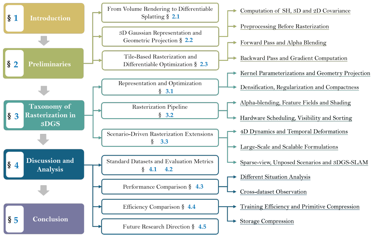
Figure 1.
Structural overview and algorithmic taxonomy of our survey. We systematically deconstruct the 3D Gaussian Splatting (3DGS) framework into a fine-grained hierarchy. Following the theoretical foundations, we categorize recent advancements into a three-tiered rasterization taxonomy: Representation and Optimization, Rasterization Pipeline, and Scenario-Driven Rasterization Extensions. Finally, we provide comprehensive cross-dataset evaluations (blue) and outline critical future research directions.
Figure 1.
Structural overview and algorithmic taxonomy of our survey. We systematically deconstruct the 3D Gaussian Splatting (3DGS) framework into a fine-grained hierarchy. Following the theoretical foundations, we categorize recent advancements into a three-tiered rasterization taxonomy: Representation and Optimization, Rasterization Pipeline, and Scenario-Driven Rasterization Extensions. Finally, we provide comprehensive cross-dataset evaluations (blue) and outline critical future research directions.
2. Preliminaries: Foundations of 3D Gaussian Splatting
This section reviews the historical evolution of explicit rendering and the core mechanics of the 3DGS differentiable rasterization pipeline.
2.1. From Volume Rendering to Differentiable Splatting
Novel view synthesis is founded on the volume rendering integral [13,14], which NeRF [3] approximates via expensive backward ray tracing. Splatting [1,15] avoids this by forward-mapping primitives and accumulating them in depth order. Point-based graphics [16,17] model complex geometries without meshes. Early systems [18,19,20] used bounding sphere hierarchies but suffered from gaps and aliasing. Surface Splatting [21,22] and EWA Splatting [23,24] introduced anisotropic Gaussian kernels, acting as low-pass filters during projection to eliminate aliasing and handle irregular sampling [25]. Although efficient on GPUs [26], these classical pipelines lacked gradient-based optimization.
Differentiable rendering [27] bridged explicit graphics and deep learning. Mesh-based methods such as OpenDR [28], Soft Rasterizer [29], and neural inverse renderers [30,31] demonstrated 3D property optimization via image-space gradients, while neural rendering [11] explored volumetric implicit representations [32,33,34]. NPBG [35] imbued point primitives with learnable features, replacing traditional shading [36]. Point-NeRF [37], SynSin [38] and Stable View Synthesis [39] combined neural features with point clouds, while Pulsar [40] and ADOP [41] developed efficient sphere-based differentiable rasterizers. However, these methods still relied on CNNs for hole-filling, limiting real-time performance.
A 3DGS scene is typically bootstrapped from a sparse Structure-from-Motion (SfM) point cloud [42,43,44,45], after which its geometric and photometric parameters are jointly refined. 3DGS [8] revitalizes EWA Splatting in a differentiable framework [46,47] for a pure explicit formulation. It allows anisotropic 3D Gaussians to jointly optimize their geometry, opacity and spherical harmonics via gradient descent, achieving state-of-the-art volumetric fidelity at real-time rasterization speed. This architecture continues to inspire specialized hardware accelerators [48], foveated VR rendering [49], and inverse rendering tasks [50,51].
Figure 2.
Illustration of the tile-based rasterization rendering process. The image plane is divided into a grid of distinct tiles. When a 3D Gaussian projected onto the 2D screen overlaps multiple tiles, it is duplicated for each intersected tile and assigned a unique sorting key in the format of [Tile ID | Depth]. These duplicated instances are subsequently sorted by depth within each tile to ensure correct visibility ordering. Finally, a thread block is assigned to each tile to perform per-pixel alpha blending, computing the cumulative transmittance and final pixel color where the evaluated opacity of a Gaussian at a specific pixel x is given by .
Figure 2.
Illustration of the tile-based rasterization rendering process. The image plane is divided into a grid of distinct tiles. When a 3D Gaussian projected onto the 2D screen overlaps multiple tiles, it is duplicated for each intersected tile and assigned a unique sorting key in the format of [Tile ID | Depth]. These duplicated instances are subsequently sorted by depth within each tile to ensure correct visibility ordering. Finally, a thread block is assigned to each tile to perform per-pixel alpha blending, computing the cumulative transmittance and final pixel color where the evaluated opacity of a Gaussian at a specific pixel x is given by .
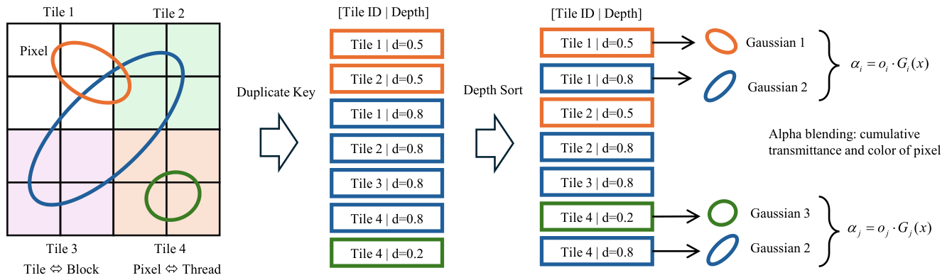

Table 1.
Deconstruction of the 3DGS Differentiable Rasterization Pipeline.
| Pipeline Stage | Core Operation | Primary Bottleneck | Related Method Types |
|---|---|---|---|
| Projection | 3D covariance to 2D footprint | Aliasing, distortion | Mip-Splatting, 3DGUT |
| Tile Binning | Duplicate Gaussians to tiles | Memory traffic | Speedy-Splat, FastGS, Taming-3DGS |
| Sorting | Per-tile depth order | Latency, popping artifacts | StopThePop, PGSR, StochasticSplats |
| Blending | Alpha accumulation | Transparency, semantic blending | Vol3DGS, LangSplat, 3DGS-Ray-Tracing |
| Backward Pass | Gradient accumulation | Atomic operations | Mini-Splatting, 2DGS |
2.2. 3D Gaussian Representation and Geometric Projection
3DGS parameterizes a scene as an unstructured ensemble of N anisotropic 3D Gaussians. Each primitive is defined by a mean position , a covariance matrix , a scalar opacity , and Spherical Harmonics (SH) color coefficients [8]. The spatial influence of a Gaussian at is evaluated as:
To ensure remains positive semi-definite during optimization, it is analytically decomposed into a learnable diagonal scaling matrix and a rotation matrix (derived from a unit quaternion ): .
During the forward pass, these 3D primitives are projected onto the 2D image plane. Given a viewing transformation and the Jacobian of the affine approximation of the perspective projection, the 3D covariance is mapped to screen space as [23]. To ensure numerical stability and prevent aliasing from sub-pixel primitives, a low-pass filter is applied by augmenting the diagonal: . The projected 2D Gaussian weight at pixel with 2D mean is:
Standard 3DGS absorbs the normalization constant into the opacity . For rigorous energy conservation during scaling, methods like Mip-Splatting [52] introduce a compensatory factor: .
2.3. Tile-Based Rasterization and Differentiable Optimization
To achieve real-time rendering speeds, 3DGS utilizes a highly optimized tile-based rasterizer. The image plane is uniformly partitioned into macro-tiles.
Initially, 3D Gaussians are frustum-culled. Surviving primitives are assigned to overlapping screen tiles and sorted by view-space depth using a fast device-side radix sort [53]. For rendering, a CUDA thread block is assigned to each tile. Threads cooperatively fetch sorted Gaussians and accumulate the final pixel color via iterative -blending:
Thread execution terminates early when the accumulated transmittance drops below a designated threshold.
During the backward pass, gradients propagate from the image-space loss through the blending chain. For a Gaussian k, gradients with respect to color and opacity are accumulated across all affected pixels using CUDA atomicAdd operations. Simultaneously, screen-space gradients for the 2D mean and covariance are derived via the chain rule on (2), and backpropagated through the viewing transform to explicitly update the 3D position , scaling , and rotation . This fully differentiable loop enables rapid, end-to-end refinement of the scene geometry and appearance.
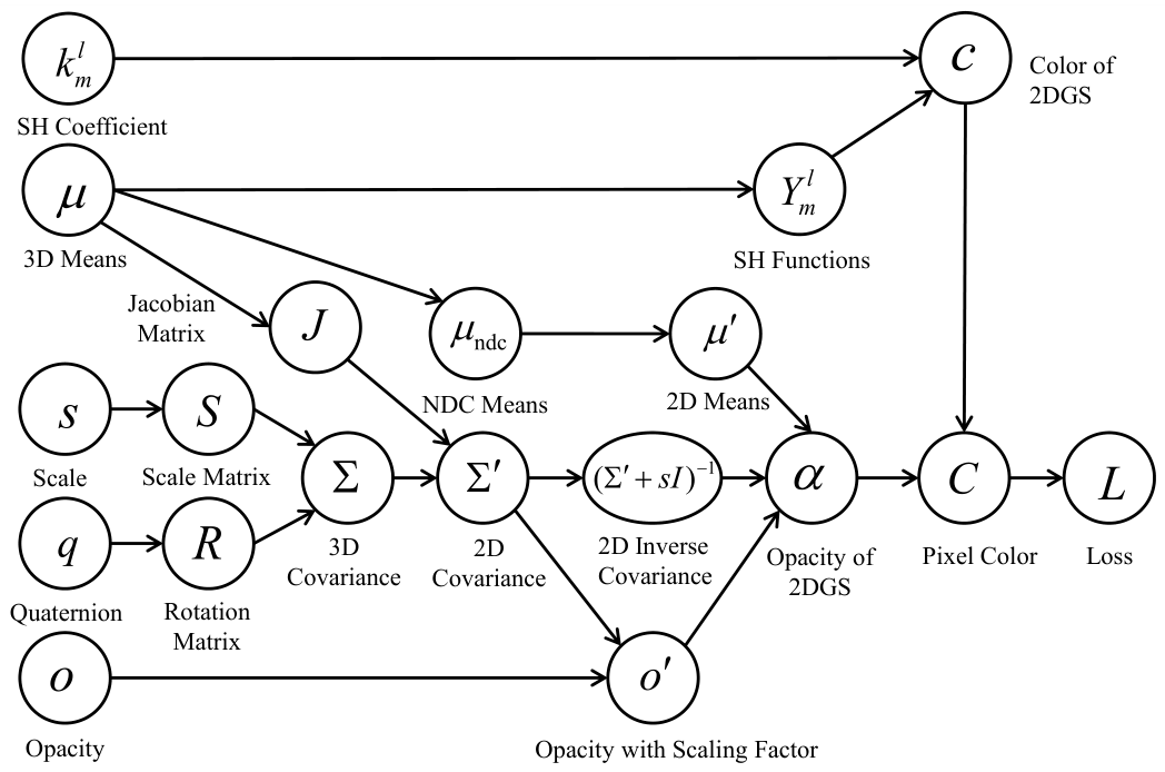
Figure 3.
The computational graph of the backward pass. The computational graph detailing the forward rendering pipeline and the backpropagation path. This directed acyclic graph illustrates how the final rendering loss L is derived from the learnable parameters of the splats. The primary optimized variables include the 3D means , spherical harmonics (SH) coefficients , scale s, quaternion q, and base opacity o. The graph demonstrates the intermediate transformations required for rendering, such as constructing the 3D covariance matrix from the scale matrix S and rotation matrix R, projecting it to the 2D covariance using the Jacobian matrix J, and computing the 2D opacity and final pixel color C. During training, the gradients flow backward through these explicit differentiable nodes to update the Gaussian parameters.
Figure 3.
The computational graph of the backward pass. The computational graph detailing the forward rendering pipeline and the backpropagation path. This directed acyclic graph illustrates how the final rendering loss L is derived from the learnable parameters of the splats. The primary optimized variables include the 3D means , spherical harmonics (SH) coefficients , scale s, quaternion q, and base opacity o. The graph demonstrates the intermediate transformations required for rendering, such as constructing the 3D covariance matrix from the scale matrix S and rotation matrix R, projecting it to the 2D covariance using the Jacobian matrix J, and computing the 2D opacity and final pixel color C. During training, the gradients flow backward through these explicit differentiable nodes to update the Gaussian parameters.
3. Taxonomy of 3DGS Rasterization Algorithms
We now present a structured algorithmic taxonomy of the 3DGS research landscape. Rather than categorizing by end-use application, we provide a viewpoint based on the specific rasterization and optimization sub-problems they address.
3.1. Representation and Optimization
3.1.1. Kernel Parameterizations and Geometry Projection
Alternative Geometric Distributions
The elliptically anisotropic 3D Gaussian serves as the fundamental primitive for standard 3DGS. However, its ellipsoidal symmetry, infinite support, and soft exponential decay often precipitate artifacts when modeling sharp edges or topologically complex boundaries. As shown in Figure 4, this inherent limitation has catalyzed a rich landscape of alternative kernel representations and projection strategies. GES [54] replaces the Gaussian kernel with a generalized exponential function that provides tighter support and sharper falloff. The kernel is defined as
where the shape parameter controls the decay rate. For , this recovers the standard Gaussian. 3DHGS [55] models each primitive as a truncated Gaussian:
where is a learnable normal direction. The hard cut introduces a true discontinuity, allowing the method to capture razor-sharp edges without blurring. 3D Student Splatting [56] generalizes the Gaussian to a Student’s t-distribution, whose heavy tails make it robust to outliers and offer more flexible shape control through the degrees of freedom. Moving beyond ellipsoids, 3D Convex Splatting [57] represents each primitive as a smooth convex polyhedron defined by the intersection of K half-spaces, allowing compact representation of complex geometries with sharp creases. Similarly, Deformable Beta Splatting uses a beta distribution density, , to enable richer deformation fields that can bend and stretch while maintaining a closed-form projection [58]. QuadBox [59] replaces the Gaussian with a geometry-aware bounding box, where the influence is defined by the smoothed distance to the box surface which accelerates rasterization as box-ray intersections are cheaper than Gaussian evaluations. N-Dimensional Gaussians lift the representation to a generic D-dimensional space, enabling joint modeling of appearance, geometry, and other attributes with a single kernel:
with the projection onto the image plane defined by marginalizing the extra dimensions [60]. 3D Skew Gaussian Splatting [61] employs a skew-normal distribution to better represent asymmetrical scattering and complex radiance fields:
where is the CDF of normal distribution, is the Cholesky factor, and the skew vector adds directional asymmetry.
Surface and Planar Approximations
To better approximate surfaces, several works collapse one dimension of the 3D Gaussian, effectively turning it into a 2D surfel. SUGAR [62] explicitly aligns Gaussian primitives with a mesh surface by adding a regularization term that encourages the shortest-axis of the covariance to align with the surface normal. Gaussian Opacity Fields (GOF) [63] proposes a paradigm shift: instead of densifying the Gaussian cloud to fill volumes, it directly models a continuous opacity field from the Gaussians and extracts a surface at the level set . The opacity field is defined as a smooth approximation of the maximum contribution from all Gaussians:
This formulation enables efficient adaptive surface reconstruction in unbounded scenes, dramatically reducing the number of required primitives. 2D Gaussian Splatting (2DGS) replaces the 3D covariance with a planar one, , which concentrates all density on a disk. This enables a geometrically consistent extraction of depth and normal via the point-to-plane distance:
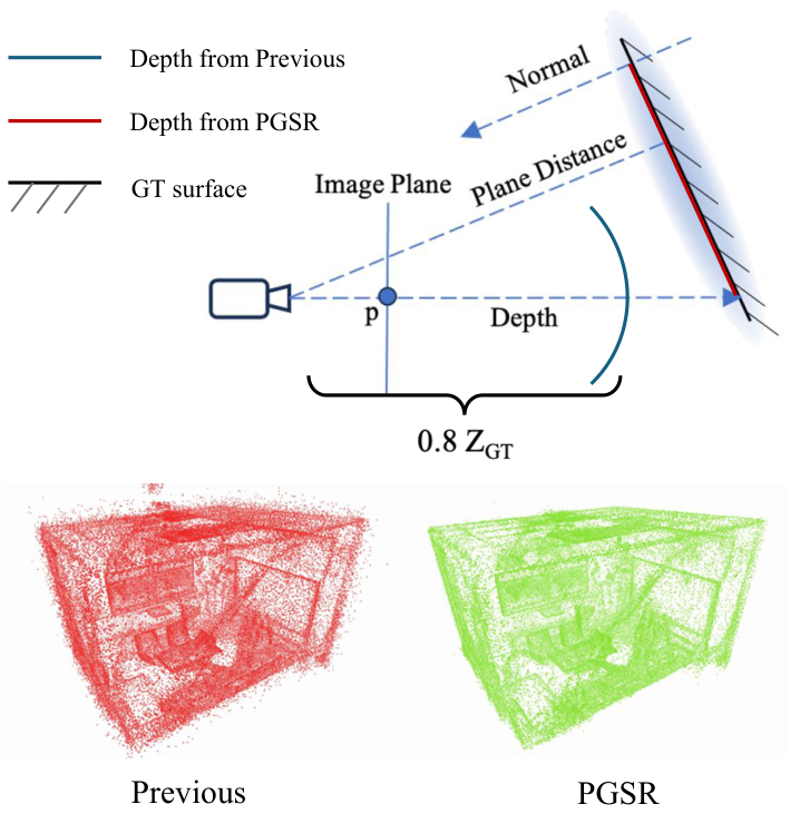
greatly improving surface alignment [64]. As shown in Figure 8, PGSR employs planar Gaussians that simplify the projection and rasterization steps, leading to more regular memory access patterns and higher efficiency on existing hardware [65]. UniGS [66] proposes a unified geometry-aware framework that jointly optimizes the Gaussian parameters and a signed distance field, using the SDF as an additional regularizer to improve densification and reconstruction accuracy across multiple modalities. Gabor Splatting [67] uses a Gabor wavelet, which is a product of a Gaussian and a sinusoid and provides a stronger response to oriented textures and high-frequency surface details.
Anti-Aliasing and Generalized Projections
Point-sampled evaluation of the Gaussian footprint triggers severe high-frequency aliasing during extreme zoom-outs. Mip-Splatting [52] mitigates aliasing by constraining the 3D frequency content of each Gaussian. It enforces that the largest scale of the covariance satisfies
where is the pixel footprint and f is a frequency factor, effectively applying a 3D low-pass filter. Analytic-Splatting [68] pushes this further by replacing the point sample with an approximate integral of the 2D Gaussian over the pixel square . 3DGUT [69] generalizes the projection model to handle distorted cameras and secondary rays. Instead of a pinhole projection , it defines a per-pixel ray function and samples the Gaussian along that ray, thereby making the rendering compatible with non-conventional optics. ODGS [70] reconstructs scenes from omnidirectional images by adjusting the projection to a spherical camera model and using feature blending that accounts for the 360° field of view. Multi-Scale 3DGS [71] addresses aliasing in unbounded scenes by building a mip-map pyramid of Gaussians. At rendering time, the appropriate level-of-detail l is selected based on the projected pixel size, and the blending function becomes a combination of scales. Multi-Sample Anti-Aliasing directly supersamples each pixel and averages the contributions [72], while Efficient Differentiable Hardware Rasterization designs dedicated GPU circuits that perform analytic anti-aliasing on the fly [73]. Physical adversarial camouflage [74] generation via 3DGS leverages the differentiability of the projection to perturb the color and texture of Gaussians, solving a min-max optimization over the rendered views under varying viewpoints.
Overall, these kernel-level designs trade the simplicity and hardware efficiency of standard Gaussian splats for greater geometric expressiveness. Different kernel designs can improve robustness and asymmetry modeling, but often require more complex projection and integration in the rasterization pipeline.
Figure 5.
Effect of collapsing 3D Gaussians into 2D splats and 3DGS’s depth simplification: (a) Integrating Gaussians along view rays r requires careful consideration of potentially overlapping 1D Gaussians. (b) Using flattened 2D splats and view-space z as depth (projection of onto v) puts 2D splats on spherical segments around the camera, inverting the relative positions of the two Gaussians along the example view ray. (c) Camera rotation inverts the order along r, resulting in popping. (d) Camera translation does not alter the distance compared to (b).
Figure 5.
Effect of collapsing 3D Gaussians into 2D splats and 3DGS’s depth simplification: (a) Integrating Gaussians along view rays r requires careful consideration of potentially overlapping 1D Gaussians. (b) Using flattened 2D splats and view-space z as depth (projection of onto v) puts 2D splats on spherical segments around the camera, inverting the relative positions of the two Gaussians along the example view ray. (c) Camera rotation inverts the order along r, resulting in popping. (d) Camera translation does not alter the distance compared to (b).

3.1.2. Densification, Regularization and Compactness
The structural evolution of a 3DGS scene relies on a coupled loop of forward rendering and adaptive density control. Standard discrete topological changes are susceptible to exploding primitives and massive memory footprints. Recent research refines these dynamics to enforce stability and extreme compactness.
Probabilistic and Perceptual Densification
The original densification heuristic relies on the noisy magnitude of positional gradients. 3DGS-MCMC [75] reinterprets the Gaussian cloud as a set of samples from an underlying probability distribution and uses Markov Chain Monte Carlo sampling to guide the life cycle of primitives. Specifically, it proposes a Metropolis–Hastings step where a new Gaussian is spawned at position with probability proportional to the rendering error:
and prunes Gaussians with low expected contribution according to a Markov chain equilibrium. This probabilistic framework helps to explore regions with unknown gradients during training, yielding more efficient and artifact-free clouds. Perceptual-GS [76] replaces the simple gradient threshold with a scene-adaptive perceptual signal. It computes a local perceptual error map using a lightweight vision-transformer head and densifies only in regions where SSIM falls below a dynamic threshold, significantly improving detail in visually salient areas. GaussianPro [77] introduces a progressive propagation strategy that expands the Gaussian cloud in a fronto-parallel manner, ensuring smooth expansion and better coverage.
Regularization and Artifact Reduction
To prevent overfitting and high-frequency artifacts during training, FreGS [78] applies progressive frequency regularization to the primitives, while Faster-GS [79] finds that gradient updates for the scaling and rotation parameters often oscillate due to a poorly conditioned learning rate ratio. They address this by rescaling the scaling gradient with the inverse of the current scale, which stabilizes convergence and cuts training time by nearly half. ABSGS [80] tackles the problem of fine detail recovery that is smoothed out during optimization. The reconstructed image is compared against the ground truth with a high-pass filter, and only the high-frequency residuals are back-propagated, effectively sharpening edges and thin structures.
Sparsification and Model Compression
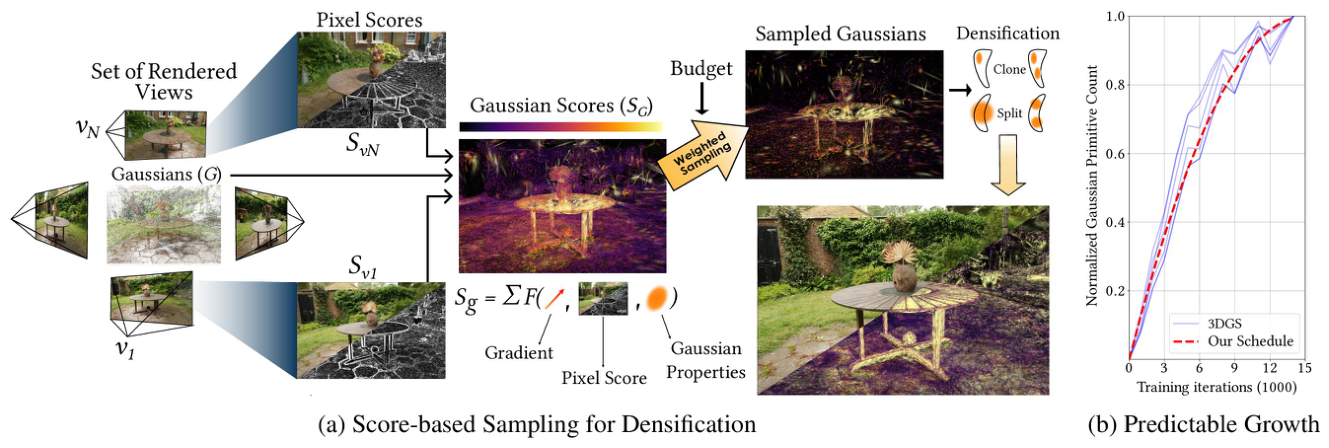
To explicitly bound memory footprints and accelerate training, recent methods aggressively prune redundancy. Mini-Splatting [81] explicitly constrains the total number of Gaussians by imposing a hard limit and formulating the optimization as a mixed integer problem. It iteratively prunes the least important Gaussians and splits the most important ones, keeping the total count constant. Taming 3DGS [82] explores a spectrum of resource-efficiency trade-offs, from predictable schedule to adaptive importance guidance as shown in Figure 9, enabling high-quality rendering on consumer-grade GPUs. LightGaussian [83] compresses the Gaussians by factorizing the SH parameter and applying a structured pruning strategy, achieving over 200 FPS with slight quality loss. RTGS [84] applies a multi-level redundancy reduction strategy that removes Gaussians based on both spatial overlap and temporal consistency. Speedy-Splat [85] accelerates both training and rendering by simultaneously applying pixel-sparse sampling and primitive-sparse selection as shown in Figure 6. GaussianSPA [86] proposes an optimizing-sparsifying loop that interleaves standard training with a sparsification operator, removing redundant primitives while boosting the influence of the remaining collection. Shorter Gaussian Lists [87] investigates training from a tiny initial set of Gaussians, showing that careful initialization and regularization help achieve comparable quality and accelerated pipeline. FastGS [88] re-engineers the entire training loop to finish optimization. It employs a dynamic sparse rasterization that skips tiles with negligible transmittance, combined with a fast gradient checkpointing scheme that recomputes only the necessary intermediate values. MMGS [89] treats the compression of 3D Gaussian as an optimal transport problem, learning a compact set of summary Gaussians that best represent the original cloud under multi-view ranking constraints The optimization minimizes the Wasserstein distance between the original and compressed sets:
maintaining rendering quality with only 10% primitives and 10× accelerated training speeds compared to 3DGS.
Feed-Forward and Initialization Strategies
Finally, a distinct subset of methods completely bypasses or drastically shortens the per-scene gradient descent loop. MVSplat [90] trains a feed-forward deep neural network to directly regress 3DGS parameters from sparse multi-view images in a single pass. Alternatively, RadSplat [91] leverages the robust initialization of NeRF to generate a highly accurate dense point cloud, which is subsequently converted into Gaussians. This hybrid approach circumvents the topological pitfalls of raw SfM initialization, achieving unprecedented 900+ FPS rendering with high quality.
In summary, densification methods improve coverage and high-frequency details, whereas pruning and compression methods reduce memory and training cost. The central challenge is to balance adaptive primitive growth with stable optimization and bounded resource consumption.
3.2. Rasterization Pipeline
With the underlying representations optimized, the computational bottleneck shifts to the execution logic on the GPU. This section dissects the rasterization pipeline, detailing innovations in physically-based shading, semantic feature blending, and low-level hardware thread scheduling.
3.2.1. Alpha Blending, Feature Fields and Shading
Physically-Based Shading and Relighting
The alpha blending algorithm in the rendering stage is not only a compositing step but also a framework that can be redesigned to incorporate complex light transport or semantic features, enabling physically based shading, open-vocabulary segmentation, and even interactive question answering. The original 3DGS uses a view-dependent spherical harmonics color model, which fails to represent specular reflections, glossy materials, and global illumination. A major paradigm shift is embedding physically-based material properties into each Gaussian for deferred shading. Relightable 3DGS [92] decomposes the outgoing radiance into a BRDF integration that respects material parameters. For a given view direction and an incident lighting direction , the reflected radiance is computed using the microfacet Cook-Torrance BRDF:
where is the half vector, and G denote the normal distribution function, Fresnel term and geometry term. The PBR color of each Gaussian is then given by:
where denotes the solid angle associated with the sampled incident direction. To compute direct illumination from a point source, the method traces secondary rays from each Gaussian to the light, evaluating a shadow map. This enables relighting the entire scene under novel illumination conditions while preserving real-time performance during view synthesis. GaussianShader [93] takes a similar approach but simplifies the BRDF to a neural shader that predicts specular and diffuse components directly from the view direction and a learnable material feature. GS-IR [94] performs inverse rendering by jointly optimizing the Gaussian geometry and an environment light probe, using the differentiable rasterizer to backpropagate gradients through the rendering equation. Geo-Splatting [95] guides the inverse rendering process with explicit geometric priors, adding a normal consistency loss between the Gaussian normals and a monocular depth estimator, which improves material decomposition.
Volumetric Consistency and Textures
Standard 3DGS blending treats each Gaussian as an independent emitter, which violates physical absorption-emission models for heterogeneous transparent media and implausible transparency effects. Don’t Splat your Gaussians [96] introduce volumetric ray-traced primitives with closed-form transmittance for efficient media rendering. 3d gaussian ray tracing [97] uses hardware-accelerated ray tracing via BVH and bounding meshes for semi-transparent particles. As shown in Figure 7, Vol3DGS [98] enforces that the alpha blending equation exactly satisfies the front-to-back absorption-emission model. It derives the discrete compositing as an unbiased Monte Carlo estimator of the continuous integral:
By introducing a continuous density field along the ray, the method resolves artifacts in scenes with semi-transparent objects. The necessity of volumetric accuracy is discussed by [99], who find that for purely opaque scenes the approximation is sufficient, but transparent and heterogeneous media benefit from the correction. Textured Gaussians [100] abandons SH coefficients in favor of explicit 2D textures mapped onto each primitive. The color of a Gaussian is sampled from the texture according to its local UV coordinates, enabling high-frequency appearance details without increasing the number of primitives. Neural Texture Splatting [101] further encodes textures as small neural networks evaluated at the Gaussian coordinates, which can also be deformed to model dynamic appearances and fine geometric displacements.
Semantic and Vision-Language Features
The speed of the 3DGS rasterizer makes it an ideal platform for distilling 2D vision-model features into a 3D representation. Feature-3DGS [102] and LangSplat [103] pioneer this direction by adding a high-dimensional feature vector to each Gaussian, which is used to render a feature map through alpha-blending:
The resulting 2D feature map can then be decoded by a segmentation head or compared against text embeddings from CLIP, enabling open-vocabulary semantic segmentation in real time. Language Embedded 3D Gaussians [104] expands this to full scene understanding, encoding not only pixel-level features but also object-level embeddings for phrase grounding. SplatTalk [105] and 3D Vision-Language GS [106] take the feature blending further by projecting vision-language models into the 3DGS framework. They train a joint embedding space where the rendered feature map can be queried with natural language, enabling tasks like 3D visual question answering and zero-shot semantic reasoning. NG-GS [107] uses a pretrained NeRF as a teacher to guide the feature distillation, improving the alignment between geometry and semantics. Fast-SegSim [108] adapts the feature rendering pipeline for robotics simulation, achieving real-time open-vocabulary segmentation by fusing 3DGS with a lightweight 2D segmentation network. LeafFit [109] applies 3DGS to create digital plant assets, leveraging the alpha blending and feature fields to accurately reconstruct translucent leaf structures. SeqAffordSplat [110] performs sequential affordance reasoning on the 3DGS representation, where the rendered feature fields encode interaction probabilities over time, allowing robots to plan actions in the rendered 3D scene.
3.2.2. Hardware Thread Scheduling, Visibility and Sorting
Sorting Elimination and Hierarchical Binning
The tile-based rasterizer of 3DGS achieves remarkable speed through a tight co-design with GPU hardware, but it also introduces bottlenecks in per-tile depth sorting, workload imbalance, and memory access. Research in this domain addresses these low-level mechanisms directly, often by reformulating the visibility problem or redesigning the rendering schedule. The per-tile radix sort is a major contributor to rendering latency. When the sorting results are retained, its efficiency becomes paramount. StochasticSplats [111] removes this step by applying stochastic transparency: each Gaussian is probabilistically accepted or discarded along the ray according to a random decision, producing a sort-free compositing that is hardware-friendly. AAA-Gaussians [112] eliminates sorting analytically by pre-integrating the alpha blending equation; it computes an equivalent order-independent transparency through a rational polynomial approximation of the visibility term, thereby suppressing popping artifacts without per-pixel depth sorting. StopThePop [113] observes that a global sort per tile often leads to view-inconsistent popping when Gaussian depths change across frames. As shown in Figure 5, it proposes a hierarchical sort that first groups Gaussians into coarse depth bins and then sorts only within the bin that covers the depth discontinuities. DistWar [114] accelerates sorting by exploiting the hardware accelerated visibility ordering in the rasterizer to perform a fast depth test and bypass the CUDA radix sort.
Hardware-Algorithm Co-Design
To maximize GPU utilization, rendering logic is increasingly co-designed with hardware primitives. GS-TG [115] proposes a tile-grouping architecture that merges adjacent tiles into larger work units, reducing redundant sorting and improving data reuse within GPU streaming multiprocessors. GauRast [116] augments standard triangle rasterizers with dedicated units for Gaussian projection and blending, achieving an order of magnitude speedup in the rasterization stage. GSAcc [117] introduces a depth-speculation mechanism that predicts per-tile depth ranges, enabling early culling of occluded Gaussians before sorting. GEMM-GS [118] maps the alpha-blending and sorting operations to a sequence of General Matrix Multiplications (GEMMs). The per-tile blending becomes a matrix multiplication where contains the Gaussian attributes and the pixel-wise accumulation weights.
Deployment Architectures and Edge Rendering
To support constrained environments, pipeline execution can be re-engineered. gsplat [119] continuously integrates low-level scheduling optimizations into a unified high-performance API. FlashGS [120] focuses on accelerating the forward process by partitioning the screen into finer tiles and scheduling them on a multi-GPU pipeline. Mobile-GS [121] brings real-time Gaussian splatting to smartphones for resource-constrained deployments by adopting a memory-centric rendering design. It loads only the Gaussians visible in the current view frustum from flash storage, uses a quantized integer representation for positions and colors, and performs the blending in a lower-precision shader.
Figure 8.
Unbiased depth rendering. (a) Illustration of the rendered depth: We take a single Gaussian, flatten it into a plane, and fit it onto the surface as an example. PGSR’s rendered depth is the intersection point of rays and surfaces, matching the actual surface. In contrast, the depth from previous methods corresponds to a curved surface and may deviate from the actual surface. (b) PGSR uses true depth to supervise two different depth rendering methods. After optimization, PGSR maps the positions of all Gaussian points. Gaussians of our method fit well onto the actual surface, while the previous method results in noise and poor adherence to the surface.
Figure 8.
Unbiased depth rendering. (a) Illustration of the rendered depth: We take a single Gaussian, flatten it into a plane, and fit it onto the surface as an example. PGSR’s rendered depth is the intersection point of rays and surfaces, matching the actual surface. In contrast, the depth from previous methods corresponds to a curved surface and may deviate from the actual surface. (b) PGSR uses true depth to supervise two different depth rendering methods. After optimization, PGSR maps the positions of all Gaussian points. Gaussians of our method fit well onto the actual surface, while the previous method results in noise and poor adherence to the surface.
3.3. Scenario-Driven Rasterization Extensions
3.3.1. 4D Dynamics and Temporal Deformations
Deformation Fields and Splines
Dynamic 3DGS extends rasterization from a static primitive set to a time-varying primitive field. The key rasterization challenge is no longer only projecting and sorting Gaussians, but doing so under temporally varying geometry, deformation fields, and visibility orders, often via a deformation network that predicts per-frame adjustments to a canonical Gaussian cloud [6,7]. A common paradigm is to keep a canonical 3DGS model at time and learn a deformation field that, for each timestep t, predicts a displacement for every Gaussian. Deformable 3D Gaussians [122] implements this with an MLP that takes positional and temporal encodings, directly supervising with multi-view videos. 4D Gaussian Splatting [123] extends this to real-time rendering by decomposing the 4D representation into a set of time-varying 3D Gaussians, where the deformation network is replaced by a compact hex-plane encoder. SplineGS replaces the discrete per-frame deformation with a smooth spline that models the trajectory of each primitive’s center and rotation as a function of time:
where are B-spline basis functions and are control points. This ensures physically plausible, smooth motion with fewer parameters [124]. TreeSplat organizes the deformation as a mergeable tree, where each node represents a rigid part of an articulated object, and the overall deformation is computed by traversing the kinematic chain [125].
Flow, Tracking, and Control
Gaussian-Flow treats each Gaussian as a dynamic particle advected by a 3D velocity field, and the 4D reconstruction is obtained by integrating the flow over time [126]. Spacetime adds a temporal dimension to the feature field, enabling real-time interpolation of both color and geometry between keyframes [127]. Gaussian Splatting Lucas-Kanade directly applies optical flow estimation to the rendered Gaussians, using the flow to align dynamic objects across frames and improve temporal consistency [128]. Real-time 4DGS achieves interactive frame rates by building a specialized renderer that fuses static background Gaussians with a small, fast-updating set of dynamic foreground Gaussians [129]. Dynamic 3D Gaussians performs tracking by persistent dynamic view synthesis, linking the motion of each Gaussian to the movement of a corresponding 3D point in the scene [130]. SC-GS allows sparse user-provided control points to edit the dynamic scene, propagating edits across time via a learned deformation prior [131]. SpeeDe3DGS [132] accelerates deformable 3DGS by applying temporal pruning. They identify static and active Gaussians and group the dynamic parts by motion similarity to reduce the number of deformation queries. RetimeGS [133] achieves continuous-time 4D reconstruction by modeling the trajectories with a neural ODE solver, allowing frame rates to be arbitrarily adjusted at test time. Gaufre [134] introduces a temporal coherence heuristic into the tile sorting, avoiding re-sorting of Gaussians whose depth order has not changed between frames.
3.3.2. Large-Scale and Scalable Formulations
Large-scale scenes stress the rasterizer through primitive count, memory bandwidth, tile occupancy, and out-of-core data movement. Overcoming this to enable city-scale reconstruction is a major challenge, addressed via spatial partitioning with level-of-detail (LoD) and out-of-core distributed training. Earlier lessons from scaling NeRF are provided by Block-NeRF [135] and Mega-NeRF [136], which introduced spatial partitioning for neural radiance fields. MatrixCity offers a large-scale city dataset specifically designed for benchmarking scalable neural rendering methods [137].
Block-Based Partitioning
A straightforward approach to massive scenes is divide-and-conquer. VastGaussian and CityGaussian [138,139] partition large scenes into overlapping blocks, train independent 3DGS models per block, and merge them at rendering time. CityGS-X [140] extends this with a geometry-aware architecture that refines block boundaries according to building footprints, achieving highly accurate urban reconstruction.
Hierarchical and LoD Structures
To avoid rendering millions of far-away, sub-pixel Gaussians, multi-resolution structures are employed. Scaffold-GS [141] anchors scene content to a sparse voxel grid, using the grid as a scaffold to allocate Gaussians only in occupied regions, which naturally adapts to view distance and improves memory efficiency. Octree-GS [142] builds an octree over the scene, associating each node with a merged Gaussian that summarizes the radiance and opacity of its children. Hierarchical 3D Gaussian Representations [143] render very large datasets in real time by storing a multi-resolution pyramid of Gaussians. Google’s LODGE [144] introduces a level-of-detail framework for large-scale 3D Gaussian Splatting, enabling efficient rendering by dynamically selecting appropriate detail levels. Similarly, Nvidia’s HiGS [145] proposes a hierarchical rendering architecture, achieving real-time performance through adaptive level selection and efficient GPU execution. FilterGS [146] proposes a traversal-free, parallel filtering structure that selects a single scale for each Gaussian via a learned network, avoiding expensive tree traversal at render time.
Urban Scenes and Autonomous Driving
Applying 3DGS to cityscapes and street views requires handling complex semantics and dynamic objects. UrbanGS [147] targets large-scale urban scenes, combining semantic segmentation to allocate Gaussians only on building facades and road surfaces. Proxy-GS [148] uses a coarse proxy mesh to guide Gaussian placement, significantly reducing the number of Gaussians required for background regions. Generative Gaussian Splatting [149] generates unbounded 3D cities by progressively extending the Gaussian cloud outward from a given seed region with a diffusion prior. For driving scenes, Street Gaussians [150] model dynamic urban environments by associating each vehicle or pedestrian with a separate 3DGS sub-model that can be moved independently. DrivingGaussian [151] composites surrounding views from multiple cameras into a single dynamic scene, aligning the Gaussian clouds of different vehicles with their tracked trajectories.
Out-of-Core and Distributed Optimization
Grendel-GS partitions the Gaussian list across multiple GPUs, where each GPU renders its own subset of Gaussians and combines the results via inter-GPU communication at partition boundaries [152]. CLM removes the GPU memory barrier by moving Gaussian states between CPU and GPU memory during optimization, using a smart caching policy to keep the most frequently updated Gaussians on the GPU [153]. TideGS pushes the frontier to over one billion primitives by implementing a fully out-of-core optimization that streams Gaussians from disk in a view-dependent order, training on a single machine with only a fraction of the data in GPU memory [154]. Wavelet-GS compresses the SH coefficients of each Gaussian using a wavelet decomposition, discarding high-frequency components that are not visible at typical viewing distances [155]. DWTGS rethinks frequency regularization for sparse-view 3DGS, applying a discrete wavelet transform on the rendered image and penalizing the loss in the wavelet domain to encourage sharper edges [156]. Momentum-GS leverages momentum self-distillation, where a teacher model (an exponential moving average of the parameters) guides the optimization of the student, improving convergence quality for large scenes [157].
Compression via Quantization and Codebooks
Concurrently, Compressed3D [158] and Compact3D [159] introduce vector quantization and codebooks to cluster Gaussian parameters with similar values into shared codewords for more efficient storage. Building on anchor-based representation, Context-GS [160] and CompGS [161] adopt context-aware approaches that explicitly model hierarchical relationships among anchors to enhance representational capacity. Pushing this further, HAC++ [162] incorporates an interpolated hash grid to provide spatial priors for unorganized anchors, establishing a sophisticated context model for arithmetic entropy coding. Alongside academic advances, industrial-grade data formats have emerged to standardize 3DGS delivery. For example, the LCC format family has evolved from LCC11 to LCC22. The original LCC1 format already supports spatial chunking and Level-of-Detail (LoD) organization for progressive loading and large-scale scene visualization. LCC2 further refines this design by decoupling data storage from LoD partitioning, organizing scene contents through a flexible hierarchical LoD tree that can index different payload types and storage backends. Together with compact binary layout and parameter quantization, such formats can reduce storage by up to 90% compared with standard PLY files, facilitating out-of-core streaming and interactive rendering for massive scenes on WebGPU clients.
Figure 9.
Overview of Taming 3DGS method. (a) They propose a systematic redesign of 3DGS densification. To select Gaussians to densify, they sample training views and compute per-pixel saliency. A scoring function F combines gradient, saliency, and primitive properties into a per-Gaussian score. (b) The addition of new Gaussians follows a predictable schedule. They follow a growth curve that mimics 3DGS’ behavior and can be fitted to yield any desired model size after training.
Figure 9.
Overview of Taming 3DGS method. (a) They propose a systematic redesign of 3DGS densification. To select Gaussians to densify, they sample training views and compute per-pixel saliency. A scoring function F combines gradient, saliency, and primitive properties into a per-Gaussian score. (b) The addition of new Gaussians follows a predictable schedule. They follow a growth curve that mimics 3DGS’ behavior and can be fitted to yield any desired model size after training.
3.3.3. Sparse-View, Unposed Scenarios and 3DGS-SLAM
Unposed Reconstruction and Feature Matching
Simultaneous Localization and Mapping (SLAM) with 3DGS is a crucial online application that unifies camera tracking and scene reconstruction. In this setting, the differentiable rasterizer provides a direct link from camera pose parameters to photometric error, enabling joint optimization. Many techniques for pose-free and sparse-view reconstruction build on earlier NeRF-based approaches [163,164,165,166,167,168,169]. For scenarios with very few input views with unknown camera poses, the 3DGS optimization problem becomes severely ill-posed. FSGS enables real-time few-shot view synthesis by initializing the Gaussian cloud from a learned prior over a shape category, then fine-tuning with a few images [170]. COLMAP-free 3DGS eliminates the need for external SfM by jointly optimizing camera poses and Gaussian parameters from scratch, using a progressive seeding strategy that starts with a single Gaussian and grows the cloud as more poses are discovered [171]. Depth-regularized Optimization improves the quality in few-shot settings by adding a monocular depth prior as an additional supervision signal for the Gaussian positions [172]. DropoutGS [173] introduces a dropout-like mechanism into the 3DGS training loop. During each forward pass, a random subset of Gaussians is temporarily deactivated, forcing the remaining primitives to compensate and learn a more generalizable representation and substantially improves novel view synthesis in sparse-view scenarios. NexusGS further exploits epipolar geometry: it computes epipolar depth priors from a small set of sparse matches and uses them to regularize the Gaussian mean and covariance during optimization [174]. Pseudo-View Enhancement via Confidence Fusion addresses unposed sparse-view reconstruction by generating pseudo-views from an ensemble of depth-to-3D estimators and fusing them based on their confidence scores, providing a richer supervision signal [175].
3DGS-based SLAM Systems
In SLAM and unposed reconstruction, rasterization becomes part of an online optimization loop, where camera poses, Gaussian parameters, and rendering residuals must be jointly updated under tight latency constraints. MonoGS [176] pioneered the tight coupling of a 3DGS map with a camera tracking frontend. It maintains a keyframe-based Gaussian cloud and, for each incoming frame, optimizes both the camera pose and the Gaussian parameters. GS-SLAM proposes a dense visual SLAM system that allocates Gaussians only in regions with high texture, reducing memory consumption while maintaining tracking accuracy [177]. Splat-SLAM performs global bundle adjustment with loop closure detection, optimizing all camera poses and the entire Gaussian cloud simultaneously in a scalable manner [178]. RTGS [84] achieves real-time performance by applying multi-level redundancy reduction: it removes spatially overlapping Gaussians and temporarily freezes the parameters of stable regions, focusing the computation on newly explored areas. OpenGS-SLAM [179] addresses RGB-only Gaussian Splatting SLAM in unbounded outdoor scenes by using pointmap regression for robust pose estimation and jointly optimizing camera poses with the 3DGS map. S3PO-GS [180] extends 3DGS-SLAM by incorporating a global scale factor estimated from monocular depth, compensating for the scale ambiguity inherent in monocular odometry. Gigaslam [181] tackles large-scale monocular SLAM by using a hierarchical representation: a coarse global map for localization and a fine local map for detailed reconstruction. WildGS-SLAM [182] is designed for dynamic environments, introducing robust motion filtering and scene decomposition to track the camera and reconstruct static backgrounds alongside moving objects.
4. Discussion and Analysis
In this section, we summarize the common benchmarks and evaluation protocols that have become standard in the 3D Gaussian Splatting literature and provide a comprehensive analysis of the performance and efficiency of state-of-the-art 3D Gaussian Splatting methods, followed by an in-depth discussion of promising directions for future research.
4.1. Standard Datasets
This subsection organizes commonly used datasets according to their primary evaluation purpose, separating benchmarks for rendering quality, geometry reconstruction, indoor scene reconstruction, large-scale outdoor scenes, and dynamic scene modeling.
4.1.1. Static Novel View Synthesis
Static novel view synthesis is commonly evaluated on Mip-NeRF 360 [183], Local Light Field Fusion (LLFF) [184], Deep Blending [185], and Tanks and Temples [186]. Mip-NeRF 360 contains challenging unbounded scenes with large depth variation and view-dependent effects. LLFF focuses on forward-facing real-world captures with sparse input views. Deep Blending provides free-viewpoint rendering scenes, while Tanks and Temples is frequently used for both view synthesis and reconstruction-oriented evaluation.
4.1.2. Geometry and Indoor RGB-D Scene Reconstruction
Geometry-oriented evaluation commonly uses DTU [187], Tanks and Temples [186], ETH3D [188], ScanNet [189], ScanNet++ [190], Replica [191] and SUN3D [192]. DTU and ETH3D provide calibrated multi-view images with reference geometry and are widely used for multi-view stereo and surface reconstruction. Tanks and Temples provides real-world indoor and outdoor scenes with laser-scanned ground-truth geometry. ScanNet, ScanNet++, and Replica are more commonly used for indoor RGB-D reconstruction, dense geometry evaluation, and scene-level analysis.
4.1.3. Large-Scale Outdoor Scenes
Large-scale outdoor reconstruction and driving-scene rendering are commonly evaluated on KITTI [193], KITTI-360 [194], Waymo Open Dataset [195], and MatrixCity [137]. KITTI and KITTI-360 are widely used for autonomous driving and urban scene understanding. Waymo provides large-scale multi-sensor street-view sequences with dynamic objects and complex traffic scenes. MatrixCity is a synthetic city-scale dataset designed for large-scale neural rendering and reconstruction.
4.1.4. Dynamic Scene Modeling
For dynamic scene modeling and 4D novel view synthesis, the Neural 3D Video dataset [196] is a representative benchmark. It contains multi-view videos of dynamic real-world scenes and is commonly used to evaluate temporal deformation, time-dependent rendering quality, and the efficiency of dynamic 3DGS.
4.2. Evaluation Metrics
The evaluation protocol should match the target task. Rendering metrics measure image quality, geometry metrics assess reconstructed structure, and efficiency metrics quantify the computational and storage cost of the rasterization pipeline.
4.2.1. Rendering Metrics
The standard rendering metrics are PSNR, SSIM [197,198], and LPIPS [199]. PSNR measures pixel-level reconstruction fidelity, SSIM evaluates structural similarity, and LPIPS measures perceptual similarity using deep visual features. Their combination has become the de facto protocol for evaluating novel view synthesis quality in 3DGS research.
4.2.2. Geometry Metrics
For geometry reconstruction, commonly used metrics include Chamfer Distance [200], accuracy, completeness, precision, recall and F-score. Chamfer Distance measures the bidirectional discrepancy between reconstructed and reference point sets or surfaces. Accuracy measures how close the reconstruction is to the reference geometry, while completeness measures how well the reference geometry is covered. Precision, recall, and F-score are widely used in reconstruction benchmarks [186,188].
4.3. Performance Comparison
To facilitate a thorough comparison across different design choices, we evaluate representative methods on three widely adopted benchmarks: Mip-NeRF 360 [183], Tanks & Temples [186], and Deep Blending [185]. The quantitative results are summarized in Table 2. All metrics are computed following the standard evaluation protocol established by 3DGS [8], reporting PSNR, SSIM [197], and LPIPS [199]. For all methods, we conducted experiments using our unified 3D Gaussian Splatting rasterization implementation for fair comparison.
4.3.1. Kernel Representation and Primitive Design
From the upper section of Table 2, it is clear that methods that refine the geometric primitive usually outperform the standard anisotropic 3D Gaussian. Among them, 3D Student Splatting and 3D Skew Gaussian Splatting achieve the highest reconstruction quality across all datasets. These improvements stem from their more flexible kernel shapes: the heavy-tailed Student’s t-distribution provides robustness to outliers, while the skew-normal distribution captures asymmetric radiance distributions that standard Gaussians cannot represent.
Flattening-based methods such as 2DGS and 3D-HGS deliver notable improvements on structured indoor scenes but show a smaller margin on unbounded outdoor environments like Mip-NeRF 360, indicating that they are more suitable for accurate surface extraction tasks. GES, despite its computationally efficient exponential kernel, trades a modest amount of quality for faster rendering, performing on par with 3DGS on Deep Blending but lagging behind other kernel designs on the other two datasets.
4.3.2. Efficiency-Oriented and Compression Methods
The middle section of Table 2 reports methods that prioritize rendering speed and training efficiency. These approaches generally accept a controlled loss in visual quality in exchange for substantial resource savings. Mini-Splatting and FastGS stand out as the most balanced compromises: Mini-Splatting constrains the total Gaussian count through importance-based pruning while preserving competitive PSNR, and FastGS reaches high reconstruction quality despite completing training in under a hundred seconds. In contrast, LightGaussian and Taming-3DGS exhibit larger quality drops, illustrating the difficulty of maintaining fidelity under aggressive compression and limited training budgets.
MMGS attains an order-of-magnitude compression via optimal transport aggregation, retaining accuracy comparable to uncompressed baselines on Tanks & Temples. Speedy-Splat and DashGaussian both deliver real-time frame rates with moderate quality, confirming that jointly exploiting pixel sparsity and primitive sparsity is a viable strategy for interactive applications.
4.3.3. Large-Scale and Anti-Aliasing Methods
The lower section of Table 2 compares methods tailored for large-scale reconstruction or anti-aliased rendering. Wavelet-GS achieves the highest PSNR on Deep Blending, benefiting from frequency-domain compression that preserves high-frequency details while reducing storage. Scaffold-GS and Octree-GS also perform strongly, particularly on Tanks & Temples, confirming that hierarchical and voxelization-based representations effectively handle large, complex scenes.
3DGS-MCMC reaches remarkable reconstruction quality on Mip-NeRF 360, demonstrating that principled, sampling-based densification can match or even surpass hand-crafted heuristics. Mip-Splatting excels in perceptual quality with lower LPIPS scores, confirming that anti-aliasing is crucial for view synthesis. GOF and PGSR show moderate quality but provide accurate surface extraction, a feature essential for downstream tasks such as meshing and collision detection.
4.3.4. Cross-Dataset Observations
Several patterns emerge across the three benchmarks. Deep Blending typically yields the highest PSNR values because of its forward-facing, densely captured scenes. Tanks & Temples poses the greatest challenge: its large-scale outdoor environments with varying illumination and heavy occlusions stress the geometric modeling capacity of each method. Interestingly, methods with alternative kernel designs show the largest relative improvements on Tanks & Temples, suggesting that better geometric primitives are especially beneficial for complex real-world scenes.
4.4. Efficiency Comparison
Low run-time, reduced memory consumption, and compact storage are critical for deployment in resource-constrained settings such as robotics, augmented/virtual reality, and mobile devices [121]. We analyze efficiency along three metrics: primitive counts, training speed and storage reduction.
4.4.1. Gaussian Count and Training Efficiency
We visualize the efficiency trade-offs through a series of plots. Figure 10 reports the Gaussian count compression ratio together with the PSNR improvement over the original 3DGS, highlighting each method’s ability to reduce model size while maintaining or even improving rendering quality. In particular, FastGS achieves a substantial reduction in Gaussian count with almost no quality degradation, while Mini-Splatting strikes an excellent balance between pruning aggressiveness and fidelity. MMGS [89] achieves a 10× reduction via optimal transport aggregation, with a modest quality trade-off. LightGaussian [83] reduces storage but with a larger PSNR penalty, illustrating the challenge of extreme compression.
Figure 11 and Figure 12 use logarithmic axes to better separate closely clustered methods and reveal subtle trade-offs. Figure 11 plots training time against PSNR. The most efficient methods achieve training speed while remaining competitive in quality. FastGS confirms that its sparse rasterization significantly accelerates the optimization loop without incurring a substantial PSNR penalty. Figure 12 compares the final Gaussian count with PSNR, again on logarithmic axes. Most efficiency-oriented methods reduce the number of primitives by 40%–70% relative to 3DGS, yet the quality loss varies significantly. MMGS and FastGS maintain quality close to the original, while LightGaussian accepts a larger drop in exchange for compact models. This indicates that a moderate reduction in primitive count is often achievable with minimal quality impact, but extreme compression still presents an open challenge.
4.4.2. Storage Compression
Figure 13 presents the storage compression ratios achieved by several representative methods across multiple large-scale datasets, including Mip-NeRF 360, Waymo, MatrixCity, and Tanks & Temples. The original 3DGS requires approximately 700–800 MB to store a typical full-resolution scene, which is prohibitive for many applications. HAC++ [162] and PyramidGS [204] achieve impressive storage compression, reducing the model size to a 15–20× reduction while maintaining a competitive PSNR. This is accomplished through a combination of hash-based parameter encoding, structured pruning, and quantization-aware training. Several methods, including Octree-GS [142], Scaffold-GS [141], and ContextGS, reduce storage indirectly by structuring the representation hierarchically or leveraging anchor-based sparsity. Their storage requirements are typically 3–5× smaller than 3DGS while maintaining competitive quality.
4.4.3. Summary of Efficiency Trends
Several key observations can be drawn from this analysis. First, the frontier of efficient 3DGS is advancing rapidly: multiple methods now achieve substantial reductions in training time, primitive count, and storage size without catastrophic quality loss. Second, there is a consistent trade-off between compression ratio and visual quality, but different techniques are pushing the frontier outward. Third, the most successful efficiency methods combine algorithmic innovations like sparse rasterization with implementation-level optimizations such as quantization and gradient clipping. This co-design philosophy is likely to drive further progress toward practical, real-time 3D Gaussian Splatting in everyday devices.
4.5. Future Research Directions
Building upon our rasterization-centric analysis, we identify several critical trajectories for future research, shifting the focus from application-level adaptations to rasterization pipeline innovations.
4.5.1. Sort-Free and Order-Robust Visibility Modeling
The per-tile radix sorting of millions of primitives constitutes a severe latency bottleneck in the current 3DGS pipeline. Furthermore, strict depth ordering frequently induces "popping" artifacts and struggles with complex semi-transparent surfaces. A paramount direction for future rasterizers is the development of sort-free or order-robust visibility modeling. Future frameworks must bypass brute-force sorting, formulating probabilistic or approximate blending mechanisms that maintain geometric fidelity while ensuring strict temporal consistency.
4.5.2. Differentiable Rasterization for Dynamic Visibility
Transitioning explicit representations to 4D dynamics and online SLAM environments introduces profound temporal visibility challenges. Currently, the continuous insertion and deformation during online updates disrupts tile-based memory coherency and necessitates costly global re-sorting. Future rasterization algorithms must natively support dynamic visibility, enabling asynchronous updates to the Gaussian representation. Furthermore, under unposed or sparse-view conditions, the pipeline must robustly propagate gradients to dynamic pose injections and handle depth uncertainty without catastrophic memory fragmentation.
4.5.3. Hardware-Aware Gaussian Rendering Primitives
While algorithmic compression is vital, the theoretical lower bound of rendering latency is strictly governed by hardware utilization. GEMM-GS [118] highlights a massive untapped potential: repurposing Tensor Cores, which is originally designed for neural network inference, for explicit rendering tasks. Future advancements will heavily rely on hardware algorithm co-design, moving toward optimized memory caching and lightweight primitive parameterizations specifically tailored for energy-constrained mobile GPUs [121] and specialized rendering accelerators [116].
4.5.4. Unified Multi-Output Splatting in a Single Pass
ReconFusion [205] and Difix3D+ [206] extended generative inpainting to the 3DGS, is a fertile research direction. Current 3DGS pipelines prioritize RGB novel view synthesis. While recent works embed semantic features [102,103] or physical material properties [94], these are typically achieved through computationally expensive, post-hoc optimization passes or duplicated rendering loops. A critical architectural evolution is the realization of a unified rasterizer. Such a pipeline would simultaneously accumulate color, depth, high-frequency surface normals, semantic logits, and BRDF properties within a single forward pass, dynamically sharing intermediate visibility states to avoid linear scaling of computational costs.
4.5.5. Standardized Efficiency and Systems-Level Benchmarks
As the field of explicit volumetric rendering matures, traditional evaluation metrics limited to perceptual quality are insufficient to capture the nuanced trade-offs of rasterization algorithms. Future research necessitates the establishment of standardized, systems-level benchmarks. To comprehensively evaluate a proposed rasterization intervention, protocols must rigorously quantify peak VRAM footprint during forward/backward passes, per-tile sorting latency, storage compression efficiency, and mobile-device energy cost. This paradigm shift will ensure that algorithmic innovations translate into tangible engineering deployments.
5. Conclusion
In this survey, we presented a rasterization-centric review of 3D Gaussian Splatting, organizing recent advances according to their intervention points in the rendering data flow. By deconstructing the 3DGS pipeline into representation design, tile-based scheduling, visibility sorting, alpha blending, and hardware-aware optimization, we illuminated the fundamental principles of how rasterization algorithms shape the efficiency and scalability of modern 3DGS systems. Furthermore, through a rigorous analysis of computational bottlenecks, we demonstrated how targeted innovations in rasterization algorithms serve as the primary catalyst for performance gains across diverse tasks. Finally, we further revealed that future progress will depend not only on more expressive primitives, but also on tighter co-design among algorithms, memory layouts, and hardware execution models.
Conflicts of Interest
The authors declare that they have no known competing financial interests or personal relationships that could have appeared to influence the work reported in this paper. This work was financially supported by the National Natural Science Foundation of China (No. 62406267), Guangdong Provincial Project (No. 2024QN11X072), Guangzhou-HKUST(GZ) Joint Funding Program (No. 2025A03J3956), and Guangzhou Municipal Education Project (No. 2024312122). The funders had no role in the study design, data collection and analysis, decision to publish, or preparation of the manuscript.
References
- Cook, R.L.; Carpenter, L.; Catmull, E. The Reyes image rendering architecture. ACM SIGGRAPH Comput. Graph. 1987, 21, 95–102. [Google Scholar] [CrossRef]
- Pharr, M.; Jakob, W.; Humphreys, G. Physically based rendering: From theory to implementation; MIT Press, 2023. [Google Scholar]
- Mildenhall, B.; Srinivasan, P.P.; Tancik, M.; Barron, J.T.; Ramamoorthi, R.; Ng, R. Nerf: Representing scenes as neural radiance fields for view synthesis. Commun. ACM 2021, 65, 99–106. [Google Scholar] [CrossRef]
- Müller, T.; Evans, A.; Schied, C.; Keller, A. Instant neural graphics primitives with a multiresolution hash encoding. ACM Trans. Graph. (TOG) 2022, 41, 1–15. [Google Scholar] [CrossRef]
- Fridovich-Keil, S.; Yu, A.; Tancik, M.; Chen, Q.; Recht, B.; Kanazawa, A. Plenoxels: Radiance fields without neural networks. In Proceedings of the Proceedings of the IEEE/CVF conference on computer vision and pattern recognition; 2022; pp. 5501–5510. [Google Scholar]
- Cao, A.; Johnson, J. Hexplane: A fast representation for dynamic scenes. In Proceedings of the Proceedings of the IEEE/CVF Conference on Computer Vision and Pattern Recognition; 2023; pp. 130–141. [Google Scholar]
- Fridovich-Keil, S.; Meanti, G.; Warburg, F.R.; Recht, B.; Kanazawa, A. K-planes: Explicit radiance fields in space, time, and appearance. In Proceedings of the Proceedings of the IEEE/CVF conference on computer vision and pattern recognition; 2023; pp. 12479–12488. [Google Scholar]
- Kerbl, B.; Kopanas, G.; Leimkühler, T.; Drettakis, G.; et al. 3d gaussian splatting for real-time radiance field rendering. ACM Trans. Graph. 2023, 42, 139–1. [Google Scholar] [CrossRef]
- Yifan, W.; Serena, F.; Wu, S.; Öztireli, C.; Sorkine-Hornung, O. Differentiable surface splatting for point-based geometry processing. ACM Trans. Graph. (TOG) 2019, 38, 1–14. [Google Scholar] [CrossRef]
- Chen, G.; Wang, W. A survey on 3d gaussian splatting. ACM Comput. Surv. 2024. [Google Scholar]
- Tewari, A.; Thies, J.; Mildenhall, B.; Srinivasan, P.; Tretschk, E.; Yifan, W.; Lassner, C.; Sitzmann, V.; Martin-Brualla, R.; Lombardi, S.; et al. Advances in neural rendering. In Proceedings of the Computer Graphics Forum; Wiley Online Library, 2022; Vol. 41, pp. 703–735. [Google Scholar] [CrossRef]
- Wang, F.; Zhu, Q.; Chang, D.; Gao, Q.; Han, J.; Zhang, T.; Hartley, R.; Pollefeys, M. Learning-based multi-view stereo: A survey. IEEE Trans. Pattern Anal. Mach. Intell. 2026. [Google Scholar]
- Max, N. Optical models for direct volume rendering. IEEE Trans. Vis. Comput. Graph. 2002, 1, 99–108. [Google Scholar]
- Brebin, R.A.; Carpenter, L.; Hanrahan, P. Volume rendering. In Seminal graphics: pioneering efforts that shaped the field; 1998; pp. 363–372. [Google Scholar] [CrossRef]
- Westover, L. Footprint evaluation for volume rendering. In Proceedings of the Proceedings of the 17th annual conference on Computer graphics and interactive techniques; 1990; pp. 367–376. [Google Scholar]
- Levoy, M.; Whitted, T. The use of points as a display primitive. 1985. [Google Scholar] [PubMed]
- Kobbelt, L.; Botsch, M. A survey of point-based techniques in computer graphics. Comput. Graph. 2004, 28, 801–814. [Google Scholar] [CrossRef]
- Rusinkiewicz, S.; Levoy, M. QSplat: A multiresolution point rendering system for large meshes. In Proceedings of the Proceedings of the 27th annual conference on Computer graphics and interactive techniques; 2000; pp. 343–352. [Google Scholar]
- Grossman, J.P.; Dally, W.J. Point sample rendering. In Proceedings of the Eurographics Workshop on Rendering Techniques; Springer, 1998; pp. 181–192. [Google Scholar]
- Dachsbacher, C.; Vogelgsang, C.; Stamminger, M. Sequential point trees. ACM Trans. Graph. (TOG) 2003, 22, 657–662. [Google Scholar] [CrossRef]
- Zwicker, M.; Pfister, H.; Van Baar, J.; Gross, M. Surface splatting. In Proceedings of the Proceedings of the 28th annual conference on Computer graphics and interactive techniques; 2001; pp. 371–378. [Google Scholar]
- Pfister, H.; Zwicker, M.; Van Baar, J.; Gross, M. Surfels: Surface elements as rendering primitives. In Proceedings of the Proceedings of the 27th annual conference on Computer graphics and interactive techniques; 2000; pp. 335–342. [Google Scholar]
- Zwicker, M.; Pfister, H.; Van Baar, J.; Gross, M. Ewa splatting. IEEE Trans. Vis. Comput. Graph. 2002, 8, 223–238. [Google Scholar] [CrossRef]
- Zwicker, M.; Pfister, H.; Van Baar, J.; Gross, M. Ewa volume splatting. In Proceedings of the Proceedings Visualization; VIS’01; IEEE, 2001; pp. 29–538. [Google Scholar]
- Ren, L.; Pfister, H.; Zwicker, M. Object space EWA surface splatting: A hardware accelerated approach to high quality point rendering. In Proceedings of the Computer graphics forum; Wiley Online Library, 2002; Vol. 21, pp. 461–470. [Google Scholar] [CrossRef]
- Botsch, M.; Hornung, A.; Zwicker, M.; Kobbelt, L. High-quality surface splatting on today’s GPUs. In Proceedings of the Proceedings Eurographics/IEEE VGTC Symposium Point-Based Graphics; IEEE, 2005; pp. 17–141. [Google Scholar]
- Kato, H.; Beker, D.; Morariu, M.; Ando, T.; Matsuoka, T.; Kehl, W.; Gaidon, A. Differentiable rendering: A survey. arXiv 2020, arXiv:2006.12057. [Google Scholar] [CrossRef]
- Loper, M.M.; Black, M.J. OpenDR: An approximate differentiable renderer. In Proceedings of the European Conference on Computer Vision; Springer, 2014; pp. 154–169. [Google Scholar]
- Liu, S.; Li, T.; Chen, W.; Li, H. Soft rasterizer: A differentiable renderer for image-based 3d reasoning. In Proceedings of the Proceedings of the IEEE/CVF international conference on computer vision; 2019; pp. 7708–7717. [Google Scholar]
- Kato, H.; Ushiku, Y.; Harada, T. Neural 3d mesh renderer. In Proceedings of the Proceedings of the IEEE conference on computer vision and pattern recognition; 2018; pp. 3907–3916. [Google Scholar]
- Nimier-David, M.; Vicini, D.; Zeltner, T.; Jakob, W. Mitsuba 2: A retargetable forward and inverse renderer. ACM Trans. Graph. (ToG) 2019, 38, 1–17. [Google Scholar] [CrossRef]
- Lombardi, S.; Simon, T.; Saragih, J.; Schwartz, G.; Lehrmann, A.; Sheikh, Y. Neural volumes: Learning dynamic renderable volumes from images. arXiv 2019, arXiv:1906.07751. [Google Scholar] [CrossRef]
- Yariv, L.; Gu, J.; Kasten, Y.; Lipman, Y. Volume rendering of neural implicit surfaces. Adv. Neural Inf. Process. Syst. 2021, 34, 4805–4815. [Google Scholar]
- Verbin, D.; Hedman, P.; Mildenhall, B.; Zickler, T.; Barron, J.T.; Srinivasan, P.P. Ref-nerf: Structured view-dependent appearance for neural radiance fields. IEEE Trans. Pattern Anal. Mach. Intell. 2024, 47, 9426–9437. [Google Scholar]
- Aliev, K.A.; Sevastopolsky, A.; Kolos, M.; Ulyanov, D.; Lempitsky, V. Neural point-based graphics. In Proceedings of the European conference on computer vision; Springer, 2020; pp. 696–712. [Google Scholar]
- Whitted, T. An improved illumination model for shaded display. In Proceedings of the Proceedings of the 6th annual conference on Computer graphics and interactive techniques; 1979; p. 14. [Google Scholar]
- Xu, Q.; Xu, Z.; Philip, J.; Bi, S.; Shu, Z.; Sunkavalli, K.; Neumann, U. Point-nerf: Point-based neural radiance fields. In Proceedings of the Proceedings of the IEEE/CVF conference on computer vision and pattern recognition; 2022; pp. 5438–5448. [Google Scholar]
- Wiles, O.; Gkioxari, G.; Szeliski, R.; Johnson, J. Synsin: End-to-end view synthesis from a single image. In Proceedings of the Proceedings of the IEEE/CVF conference on computer vision and pattern recognition; 2020; pp. 7467–7477. [Google Scholar]
- Riegler, G.; Koltun, V. Stable view synthesis. In Proceedings of the Proceedings of the IEEE/CVF conference on computer vision and pattern recognition; 2021; pp. 12216–12225. [Google Scholar]
- Lassner, C.; Zollhofer, M. Pulsar: Efficient sphere-based neural rendering. In Proceedings of the Proceedings of the IEEE/CVF conference on computer vision and pattern recognition; 2021; pp. 1440–1449. [Google Scholar]
- Rückert, D.; Franke, L.; Stamminger, M. Adop: Approximate differentiable one-pixel point rendering. ACM Trans. Graph. (ToG) 2022, 41, 1–14. [Google Scholar] [CrossRef]
- Seitz, S.M.; Dyer, C.R. Photorealistic scene reconstruction by voxel coloring. Int. J. Comput. Vis. 1999, 35, 151–173. [Google Scholar] [CrossRef]
- Furukawa, Y.; Ponce, J. Accurate, dense, and robust multiview stereopsis. IEEE Trans. Pattern Anal. Mach. Intell. 2009, 32, 1362–1376. [Google Scholar] [CrossRef]
- Schönberger, J.L.; Zheng, E.; Frahm, J.M.; Pollefeys, M. Pixelwise view selection for unstructured multi-view stereo. In Proceedings of the European conference on computer vision; Springer, 2016; pp. 501–518. [Google Scholar]
- Pittaluga, F.; Koppal, S.J.; Kang, S.B.; Sinha, S.N. Revealing scenes by inverting structure from motion reconstructions. In Proceedings of the Proceedings of the IEEE/CVF Conference on Computer Vision and Pattern Recognition; 2019; pp. 145–154. [Google Scholar]
- Laine, S.; Hellsten, J.; Karras, T.; Seol, Y.; Lehtinen, J.; Aila, T. Modular primitives for high-performance differentiable rendering. ACM Trans. Graph. (ToG) 2020, 39, 1–14. [Google Scholar] [CrossRef]
- Li, T.M.; Aittala, M.; Durand, F.; Lehtinen, J. Differentiable monte carlo ray tracing through edge sampling. ACM Trans. Graph. (TOG) 2018, 37, 1–11. [Google Scholar] [CrossRef]
- Li, X.; Jiang, J.; Feng, Y.; Gan, Y.; Zhao, J.; Liu, Z.; Leng, J.; Guo, M. SLTarch: Towards Scalable Point-Based Neural Rendering by Taming Workload Imbalance and Memory Irregularity. In Proceedings of the 2025 IEEE/ACM International Conference On Computer Aided Design (ICCAD); IEEE, 2025; pp. 1–9. [Google Scholar]
- Franke, L.; Fink, L.; Stamminger, M. Vr-splatting: Foveated radiance field rendering via 3d gaussian splatting and neural points. Proc. ACM Comput. Graph. Interact. Tech. 2025, 8, 1–21. [Google Scholar] [CrossRef]
- Chung, H.G.; Choi, S.; Baek, S.H. Differentiable point-based inverse rendering. In Proceedings of the Proceedings of the IEEE/CVF Conference on Computer Vision and Pattern Recognition; 2024; pp. 4399–4409. [Google Scholar]
- Rakhimov, R.; Ardelean, A.T.; Lempitsky, V.; Burnaev, E. Npbg++: Accelerating neural point-based graphics. In Proceedings of the Proceedings of the IEEE/CVF conference on computer vision and pattern recognition; 2022; pp. 15969–15979. [Google Scholar]
- Yu, Z.; Chen, A.; Huang, B.; Sattler, T.; Geiger, A. Mip-splatting: Alias-free 3d gaussian splatting. In Proceedings of the Proceedings of the IEEE/CVF conference on computer vision and pattern recognition; 2024; pp. 19447–19456. [Google Scholar]
- Laine, S.; Karras, T. High-performance software rasterization on GPUs. In Proceedings of the proceedings of the acm siggraph symposium on high performance graphics; 2011; pp. 79–88. [Google Scholar]
- Hamdi, A.; Melas-Kyriazi, L.; Mai, J.; Qian, G.; Liu, R.; Vondrick, C.; Ghanem, B.; Vedaldi, A. Ges: Generalized exponential splatting for efficient radiance field rendering. In Proceedings of the Proceedings of the IEEE/CVF Conference on Computer Vision and Pattern Recognition; 2024; pp. 19812–19822. [Google Scholar]
- Li, H.; Liu, J.; Sznaier, M.; Camps, O. 3d-hgs: 3d half-gaussian splatting. In Proceedings of the Proceedings of the Computer Vision and Pattern Recognition Conference; 2025; pp. 10996–11005. [Google Scholar]
- Zhu, J.; Yue, J.; He, F.; Wang, H. 3d student splatting and scooping. In Proceedings of the Proceedings of the Computer Vision and Pattern Recognition Conference; 2025; pp. 21045–21054. [Google Scholar]
- Held, J.; Vandeghen, R.; Hamdi, A.; Deliege, A.; Cioppa, A.; Giancola, S.; Vedaldi, A.; Ghanem, B.; Van Droogenbroeck, M. 3D convex splatting: Radiance field rendering with 3D smooth convexes. In Proceedings of the Proceedings of the IEEE/CVF Conference on Computer Vision and Pattern Recognition; 2025; pp. 21360–21369. [Google Scholar]
- Liu, R.; Sun, D.; Chen, M.; Wang, Y.; Feng, A. Deformable beta splatting. In Proceedings of the Proceedings of the Special Interest Group on Computer Graphics and Interactive Techniques Conference Conference Papers; 2025; pp. 1–11. [Google Scholar]
- Li, X.; Yang, B.; Chen, P.; Wang, Y.; Luo, H.; Cheng, W.; Su, W. QuadBox: Accelerating 3D Gaussian Splatting with Geometry-Aware Boxes. arXiv 2026, arXiv:2605.04844. [Google Scholar] [CrossRef]
- Diolatzis, S.; Zirr, T.; Kuznetsov, A.; Kopanas, G.; Kaplanyan, A. N-dimensional gaussians for fitting of high dimensional functions. In Proceedings of the ACM SIGGRAPH 2024 Conference Papers; 2024; pp. 1–11. [Google Scholar]
- Zhao, B.; Zhou, Y.; Song, G.; Yin, Z.; Wang, H. 3D Skew Gaussian Splatting with Any Camera Trajectory Visualization Engine. arXiv 2026, arXiv:2605.18334. [Google Scholar] [CrossRef]
- Guédon, A.; Lepetit, V. Sugar: Surface-aligned gaussian splatting for efficient 3d mesh reconstruction and high-quality mesh rendering. In Proceedings of the Proceedings of the IEEE/CVF conference on computer vision and pattern recognition; 2024; pp. 5354–5363. [Google Scholar]
- Yu, Z.; Sattler, T.; Geiger, A. Gaussian opacity fields: Efficient adaptive surface reconstruction in unbounded scenes. ACM Trans. Graph. (ToG) 2024, 43, 1–13. [Google Scholar] [CrossRef]
- Huang, B.; Yu, Z.; Chen, A.; Geiger, A.; Gao, S. 2d gaussian splatting for geometrically accurate radiance fields. In Proceedings of the ACM SIGGRAPH 2024 conference papers; 2024; pp. 1–11. [Google Scholar]
- Chen, D.; Li, H.; Ye, W.; Wang, Y.; Xie, W.; Zhai, S.; Wang, N.; Liu, H.; Bao, H.; Zhang, G. Pgsr: Planar-based gaussian splatting for efficient and high-fidelity surface reconstruction. IEEE Trans. Vis. Comput. Graph. 2024, 31, 6100–6111. [Google Scholar]
- Xie, Y.; Huang, Z.; Jiao, J.; Kanoulas, D.; Ma, J. UniGS: Unified Geometry-Aware Gaussian Splatting for Multimodal Rendering. arXiv 2025, arXiv:2510.12174. [Google Scholar] [CrossRef]
- Watanabe, H.; Umetani, N. Neural Gabor Splatting: Enhanced Gaussian Splatting with Neural Gabor for High-frequency Surface Reconstruction. arXiv 2026, arXiv:2604.15941. [Google Scholar]
- Liang, Z.; Zhang, Q.; Hu, W.; Zhu, L.; Feng, Y.; Jia, K. Analytic-splatting: Anti-aliased 3d gaussian splatting via analytic integration. In Proceedings of the European conference on computer vision; Springer, 2024; pp. 281–297. [Google Scholar]
- Wu, Q.; Esturo, J.M.; Mirzaei, A.; Moenne-Loccoz, N.; Gojcic, Z. 3dgut: Enabling distorted cameras and secondary rays in gaussian splatting. In Proceedings of the Proceedings of the Computer Vision and Pattern Recognition Conference; 2025; pp. 26036–26046. [Google Scholar]
- Lee, S.; Chung, J.; Huh, J.; Lee, K.M. Odgs: 3d scene reconstruction from omnidirectional images with 3d gaussian splattings. Adv. Neural Inf. Process. Syst. 2024, 37, 57050–57075. [Google Scholar] [CrossRef]
- Yan, Z.; Low, W.F.; Chen, Y.; Lee, G.H. Multi-scale 3d gaussian splatting for anti-aliased rendering. In Proceedings of the Proceedings of the IEEE/CVF Conference on Computer Vision and Pattern Recognition; 2024; pp. 20923–20931. [Google Scholar]
- Zhou, Z.; Zhang, J.C.; Xiong, Y.J.; Xia, C.M. Multi-Sample Anti-Aliasing and Constrained Optimization for 3D Gaussian Splatting. arXiv 2025, arXiv:2508.10507. [Google Scholar] [CrossRef]
- Yuan, Y.; He, Q. Efficient Differentiable Hardware Rasterization for 3D Gaussian Splatting. arXiv 2025, arXiv:2505.18764. [Google Scholar] [CrossRef]
- Lou, T.; Jia, X.; Liang, S.; Liang, J.; Zhang, M.; Xiao, Y.; Cao, X. 3d gaussian splatting driven multi-view robust physical adversarial camouflage generation. In Proceedings of the Proceedings of the IEEE/CVF International Conference on Computer Vision; 2025; pp. 28752–28762. [Google Scholar]
- Kheradmand, S.; Rebain, D.; Sharma, G.; Sun, W.; Tseng, Y.C.; Isack, H.; Kar, A.; Tagliasacchi, A.; Yi, K.M. 3d gaussian splatting as markov chain monte carlo. Adv. Neural Inf. Process. Syst. 2024, 37, 80965–80986. [Google Scholar] [CrossRef]
- Zhou, H.; Ni, Z. Perceptual-GS: Scene-adaptive perceptual densification for Gaussian splatting. arXiv 2025, arXiv:2506.12400. [Google Scholar] [CrossRef]
- Cheng, K.; Long, X.; Yang, K.; Yao, Y.; Yin, W.; Ma, Y.; Wang, W.; Chen, X. Gaussianpro: 3d gaussian splatting with progressive propagation. In Proceedings of the Forty-first International Conference on Machine Learning; 2024. [Google Scholar]
- Zhang, J.; Zhan, F.; Xu, M.; Lu, S.; Xing, E. Fregs: 3d gaussian splatting with progressive frequency regularization. In Proceedings of the Proceedings of the IEEE/CVF Conference on Computer Vision and Pattern Recognition; 2024; pp. 21424–21433. [Google Scholar]
- Hahlbohm, F.; Franke, L.; Eisemann, M.; Magnor, M. Faster-gs: Analyzing and improving gaussian splatting optimization. arXiv 2026, arXiv:2602.09999. [Google Scholar]
- Ye, Z.; Li, W.; Liu, S.; Qiao, P.; Dou, Y. Absgs: Recovering fine details in 3d gaussian splatting. In Proceedings of the Proceedings of the 32nd ACM international conference on multimedia; 2024; pp. 1053–1061. [Google Scholar]
- Fang, G.; Wang, B. Mini-splatting: Representing scenes with a constrained number of gaussians. In Proceedings of the European conference on computer vision; Springer, 2024; pp. 165–181. [Google Scholar]
- Mallick, S.S.; Goel, R.; Kerbl, B.; Steinberger, M.; Carrasco, F.V.; De La Torre, F. Taming 3dgs: High-quality radiance fields with limited resources. In Proceedings of the SIGGRAPH Asia 2024 Conference Papers; 2024; pp. 1–11. [Google Scholar] [CrossRef]
- Fan, Z.; Wang, K.; Wen, K.; Zhu, Z.; Xu, D.; Wang, Z. Lightgaussian: Unbounded 3d gaussian compression with 15x reduction and 200+ fps. Adv. Neural Inf. Process. Syst. 2024, 37, 140138–140158. [Google Scholar] [CrossRef]
- Li, L.; Qin, J.; Peng, J.; Wan, Z.; Qu, H.; Han, Y.; Zheng, P.; Zhang, H.; Cao, Y.; Chen, T.; et al. Rtgs: Real-time 3d gaussian splatting slam via multi-level redundancy reduction. In Proceedings of the Proceedings of the 58th IEEE/ACM International Symposium on Microarchitecture; 2025; pp. 1838–1851. [Google Scholar]
- Hanson, A.; Tu, A.; Lin, G.; Singla, V.; Zwicker, M.; Goldstein, T. Speedy-splat: Fast 3d gaussian splatting with sparse pixels and sparse primitives. In Proceedings of the Proceedings of the Computer Vision and Pattern Recognition Conference; 2025; pp. 21537–21546. [Google Scholar]
- Zhang, Y.; Jia, W.; Niu, W.; Yin, M. Gaussianspa: An" optimizing-sparsifying" simplification framework for compact and high-quality 3d gaussian splatting. In Proceedings of the Proceedings of the Computer Vision and Pattern Recognition Conference; 2025; pp. 26673–26682. [Google Scholar]
- Liu, J.; Han, Z. Speeding Up the Learning of 3D Gaussians with Much Shorter Gaussian Lists. arXiv 2026, arXiv:2603.09277. [Google Scholar]
- Ren, S.; Wen, T.; Fang, Y.; Lu, B. FastGS: Training 3D Gaussian Splatting in 100 Seconds. arXiv 2025, arXiv:2511.04283. [Google Scholar]
- Zhao, B.; Yu, S.; Yin, Z.; Shen, D.; Wang, H. MMGS: 10× Compressed 3DGS through Optimal Transport Aggregation based on Multi-view Ranking. arXiv 2026, arXiv:2605.19304. [Google Scholar]
- Chen, Y.; Xu, H.; Zheng, C.; Zhuang, B.; Pollefeys, M.; Geiger, A.; Cham, T.J.; Cai, J. Mvsplat: Efficient 3d gaussian splatting from sparse multi-view images. In Proceedings of the European conference on computer vision; Springer, 2024; pp. 370–386. [Google Scholar]
- Niemeyer, M.; Manhardt, F.; Rakotosaona, M.J.; Oechsle, M.; Duckworth, D.; Gosula, R.; Tateno, K.; Bates, J.; Kaeser, D.; Tombari, F. Radsplat: Radiance field-informed gaussian splatting for robust real-time rendering with 900+ fps. In Proceedings of the 2025 International Conference on 3D Vision (3DV). IEEE; 2025; pp. 134–144. [Google Scholar]
- Gao, J.; Gu, C.; Lin, Y.; Li, Z.; Zhu, H.; Cao, X.; Zhang, L.; Yao, Y. Relightable 3d gaussians: Realistic point cloud relighting with brdf decomposition and ray tracing. In Proceedings of the European Conference on Computer Vision; Springer, 2024; pp. 73–89. [Google Scholar]
- Jiang, Y.; Tu, J.; Liu, Y.; Gao, X.; Long, X.; Wang, W.; Ma, Y. Gaussianshader: 3d gaussian splatting with shading functions for reflective surfaces. In Proceedings of the Proceedings of the IEEE/CVF conference on computer vision and pattern recognition; 2024; pp. 5322–5332. [Google Scholar]
- Liang, Z.; Zhang, Q.; Feng, Y.; Shan, Y.; Jia, K. Gs-ir: 3d gaussian splatting for inverse rendering. In Proceedings of the Proceedings of the IEEE/CVF Conference on Computer Vision and Pattern Recognition; 2024; pp. 21644–21653. [Google Scholar]
- Ye, K.; Gao, C.; Li, G.; Chen, W.; Chen, B. Geosplatting: Towards geometry guided gaussian splatting for physically-based inverse rendering. In Proceedings of the Proceedings of the IEEE/CVF International Conference on Computer Vision; 2025; pp. 28991–29000. [Google Scholar]
- Condor, J.; Speierer, S.; Bode, L.; Bozic, A.; Green, S.; Didyk, P.; Jarabo, A. Don’t Splat your Gaussians: Volumetric Ray-Traced Primitives for Modeling and Rendering Scattering and Emissive Media. ACM Trans. Graph. 2025, 44, 1–17. [Google Scholar] [CrossRef]
- Moenne-Loccoz, N.; Mirzaei, A.; Perel, O.; De Lutio, R.; Martinez Esturo, J.; State, G.; Fidler, S.; Sharp, N.; Gojcic, Z. 3d gaussian ray tracing: Fast tracing of particle scenes. ACM Trans. Graph. (TOG) 2024, 43, 1–19. [Google Scholar] [CrossRef]
- Talegaonkar, C.; Belhe, Y.; Ramamoorthi, R.; Antipa, N. Volumetrically consistent 3d gaussian rasterization. In Proceedings of the Proceedings of the IEEE/CVF Conference on Computer Vision and Pattern Recognition; 2025; pp. 10953–10963. [Google Scholar]
- Celarek, A.; Kopanas, G.; Drettakis, G.; Wimmer, M.; Kerbl, B. Does 3d gaussian splatting need accurate volumetric rendering? In Proceedings of the Computer Graphics Forum; Wiley Online Library, 2025; Vol. 44, p. e70032. [Google Scholar]
- Chao, B.; Tseng, H.Y.; Porzi, L.; Gao, C.; Li, T.; Li, Q.; Saraf, A.; Huang, J.B.; Kopf, J.; Wetzstein, G.; et al. Textured gaussians for enhanced 3d scene appearance modeling. In Proceedings of the Computer Vision and Pattern Recognition Conference; 2025; pp. 8964–8974. [Google Scholar] [CrossRef]
- Wang, Y.; Wang, S.; Mihajlovic, M.; Tang, S. Neural Texture Splatting: Expressive 3D Gaussian Splatting for View Synthesis, Geometry, and Dynamic Reconstruction. In Proceedings of the Proceedings of the SIGGRAPH Asia 2025 Conference Papers; 2025; pp. 1–12. [Google Scholar] [CrossRef]
- Zhou, S.; Chang, H.; Jiang, S.; Fan, Z.; Zhu, Z.; Xu, D.; Chari, P.; You, S.; Wang, Z.; Kadambi, A. Feature 3dgs: Supercharging 3d gaussian splatting to enable distilled feature fields. In Proceedings of the Proceedings of the IEEE/CVF Conference on Computer Vision and Pattern Recognition; 2024; pp. 21676–21685. [Google Scholar]
- Qin, M.; Li, W.; Zhou, J.; Wang, H.; Pfister, H. Langsplat: 3d language gaussian splatting. In Proceedings of the Proceedings of the IEEE/CVF Conference on Computer Vision and Pattern Recognition; 2024; pp. 20051–20060. [Google Scholar]
- Shi, J.C.; Wang, M.; Duan, H.B.; Guan, S.H. Language embedded 3d gaussians for open-vocabulary scene understanding. In Proceedings of the Proceedings of the IEEE/CVF Conference on Computer Vision and Pattern Recognition; 2024; pp. 5333–5343. [Google Scholar]
- Thai, A.; Peng, S.; Genova, K.; Guibas, L.; Funkhouser, T. Splattalk: 3d vqa with gaussian splatting. In Proceedings of the Proceedings of the IEEE/CVF International Conference on Computer Vision; 2025; pp. 4712–4721. [Google Scholar]
- Peng, Q.; Planche, B.; Gao, Z.; Zheng, M.; Choudhuri, A.; Chen, T.; Chen, C.; Wu, Z. 3d vision-language gaussian splatting. In Proceedings of the International Conference on Learning Representations; 2025; Vol. 2025, pp. 61008–61031. [Google Scholar]
- He, Y.; Wang, T.; Jin, Y.; Lang, C.; Li, Y.; Ling, H. NG-GS: NeRF-Guided 3D Gaussian Splatting Segmentation. arXiv 2026, arXiv:2604.14706. [Google Scholar]
- Yu, X.; Xie, Y.; Zhai, S.; Ye, S.; Xiong, R.; Wang, Y. Fast-SegSim: Real-Time Open-Vocabulary Segmentation for Robotics in Simulation. arXiv 2026, arXiv:2604.10951. [Google Scholar] [CrossRef]
- Luo, C.; Umetani, N. LeafFit: Plant Assets Creation from 3D Gaussian Splatting. In Proceedings of the Computer Graphics Forum; Wiley Online Library, 2026; p. e70374. [Google Scholar]
- Li, D.; Feng, J.; Chen, J.; Dong, W.; Li, G.; Zheng, Y.; Feng, M.; Shi, G. SeqAffordSplat: Scene-level Sequential Affordance Reasoning on 3D Gaussian Splatting. arXiv 2025, arXiv:2507.23772. [Google Scholar] [CrossRef]
- Kheradmand, S.; Vicini, D.; Kopanas, G.; Lagun, D.; Yi, K.M.; Matthews, M.; Tagliasacchi, A. Stochasticsplats: Stochastic rasterization for sorting-free 3d gaussian splatting. In Proceedings of the Proceedings of the IEEE/CVF International Conference on Computer Vision; 2025; pp. 26326–26335. [Google Scholar]
- Steiner, M.; Köhler, T.; Radl, L.; Windisch, F.; Schmalstieg, D.; Steinberger, M. AAA-Gaussians: Anti-Aliased and Artifact-Free 3D Gaussian Rendering. In Proceedings of the Proceedings of the IEEE/CVF International Conference on Computer Vision; 2025; pp. 27650–27659. [Google Scholar]
- Radl, L.; Steiner, M.; Parger, M.; Weinrauch, A.; Kerbl, B.; Steinberger, M. Stopthepop: Sorted gaussian splatting for view-consistent real-time rendering. ACM Trans. Graph. (TOG) 2024, 43, 1–17. [Google Scholar] [CrossRef]
- Durvasula, S.; Zhao, A.; Chen, F.; Liang, R.; Sanjaya, P.K.; Vijaykumar, N. Distwar: Fast differentiable rendering on raster-based rendering pipelines. arXiv 2023, arXiv:2401.05345. [Google Scholar] [CrossRef]
- Jo, J.; Park, J. GS-TG: 3D Gaussian Splatting Accelerator with Tile Grouping for Reducing Redundant Sorting while Preserving Rasterization Efficiency. In Proceedings of the 2025 62nd ACM/IEEE Design Automation Conference (DAC); IEEE, 2025; pp. 1–7. [Google Scholar]
- Li, S.; Keller, B.; Lin, Y.C.; Khailany, B. GauRast: Enhancing GPU triangle rasterizers to accelerate 3D Gaussian splatting. In Proceedings of the 2025 62nd ACM/IEEE Design Automation Conference (DAC); IEEE, 2025; pp. 1–7. [Google Scholar]
- Yang, M.; Wang, Y.; Lo, C.P.; Zhang, X.; Oruganti, S.; Kulkarni, J.P. GSAcc: Accelerate 3D Gaussian Splatting via Depth Speculation and Gaussian-centric Rasterization. In Proceedings of the 2025 62nd ACM/IEEE Design Automation Conference (DAC); IEEE, 2025; pp. 1–7. [Google Scholar]
- Li, H.; Zhu, B.; Liu, F.; Wang, Z.; Liang, X.; Jiang, L.; Guan, H. GEMM-GS: Accelerating 3D Gaussian Splatting on Tensor Cores with GEMM-Compatible Blending. arXiv 2026, arXiv:2604.02120. [Google Scholar] [CrossRef]
- Ye, V.; Li, R.; Kerr, J.; Turkulainen, M.; Yi, B.; Pan, Z.; Seiskari, O.; Ye, J.; Hu, J.; Tancik, M.; et al. gsplat: An open-source library for Gaussian splatting. J. Mach. Learn. Res. 2025, 26, 1–17. [Google Scholar] [CrossRef]
- Feng, G.; Chen, S.; Fu, R.; Liao, Z.; Wang, Y.; Liu, T.; Hu, B.; Xu, L.; Pei, Z.; Li, H.; et al. Flashgs: Efficient 3d gaussian splatting for large-scale and high-resolution rendering. In Proceedings of the Proceedings of the Computer Vision and Pattern Recognition Conference; 2025; pp. 26652–26662. [Google Scholar]
- Du, X.; Wang, Y.; Zhan, K.; Yu, X. Mobile-GS: Real-time Gaussian splatting for mobile devices. arXiv 2026, arXiv:2603.11531. [Google Scholar] [CrossRef]
- Yang, Z.; Gao, X.; Zhou, W.; Jiao, S.; Zhang, Y.; Jin, X. Deformable 3d gaussians for high-fidelity monocular dynamic scene reconstruction. In Proceedings of the Proceedings of the IEEE/CVF conference on computer vision and pattern recognition; 2024; pp. 20331–20341. [Google Scholar]
- Wu, G.; Yi, T.; Fang, J.; Xie, L.; Zhang, X.; Wei, W.; Liu, W.; Tian, Q.; Wang, X. 4d gaussian splatting for real-time dynamic scene rendering. In Proceedings of the Proceedings of the IEEE/CVF conference on computer vision and pattern recognition; 2024; pp. 20310–20320. [Google Scholar]
- Park, J.; Bui, M.Q.V.; Bello, J.L.G.; Moon, J.; Oh, J.; Kim, M. Splinegs: Robust motion-adaptive spline for real-time dynamic 3d gaussians from monocular video. In Proceedings of the Proceedings of the Computer Vision and Pattern Recognition Conference; 2025; pp. 26866–26875. [Google Scholar]
- Shen, Q.; Yang, X.; Wang, X. TreeSplat: mergeable tree for deformable gaussian splatting. Adv. Neural Inf. Process. Syst. 2026, 38, 137092–137111. [Google Scholar]
- Lin, Y.; Dai, Z.; Zhu, S.; Yao, Y. Gaussian-flow: 4d reconstruction with dynamic 3d gaussian particle. In Proceedings of the Proceedings of the IEEE/CVF Conference on Computer Vision and Pattern Recognition; 2024; pp. 21136–21145. [Google Scholar]
- Li, Z.; Chen, Z.; Li, Z.; Xu, Y. Spacetime gaussian feature splatting for real-time dynamic view synthesis. In Proceedings of the Proceedings of the IEEE/CVF Conference on Computer Vision and Pattern Recognition; 2024; pp. 8508–8520. [Google Scholar]
- Xie, L.; Julin, J.; Niinuma, K.; Jeni, L.A. Gaussian splatting lucas-kanade. In Proceedings of the International Conference on Learning Representations; 2025; Vol. 2025, pp. 97444–97463. [Google Scholar]
- Yang, Z.; Yang, H.; Pan, Z.; Zhang, L. Real-time photorealistic dynamic scene representation and rendering with 4d gaussian splatting. In Proceedings of the International Conference on Learning Representations; 2024; Vol. 2024, pp. 9142–9159. [Google Scholar]
- Luiten, J.; Kopanas, G.; Leibe, B.; Ramanan, D. Dynamic 3d gaussians: Tracking by persistent dynamic view synthesis. In Proceedings of the 2024 International Conference on 3D Vision (3DV). IEEE; 2024; pp. 800–809. [Google Scholar]
- Huang, Y.H.; Sun, Y.T.; Yang, Z.; Lyu, X.; Cao, Y.P.; Qi, X. Sc-gs: Sparse-controlled gaussian splatting for editable dynamic scenes. In Proceedings of the Proceedings of the IEEE/CVF conference on computer vision and pattern recognition; 2024; pp. 4220–4230. [Google Scholar]
- Tu, A.; Ying, H.; Hanson, A.; Lee, Y.; Goldstein, T.; Zwicker, M. SpeeDe3DGS: Speedy Deformable 3D Gaussian Splatting with Temporal Pruning and Motion Grouping. arXiv 2025, arXiv:2506.07917. [Google Scholar]
- Wang, X.; Ma, L.; Shen, Y.; Wang, Z.; Sander, P.V. RetimeGS: Continuous-Time Reconstruction of 4D Gaussian Splatting. arXiv 2026, arXiv:2603.13783. [Google Scholar]
- Liang, Y.; Khan, N.; Li, Z.; Nguyen-Phuoc, T.H.; Lanman, D.; Tompkin, J.; Xiao, L. Gaufre: Gaussian deformation fields for real-time dynamic novel view synthesis. In Proceedings of the Proceedings of the Winter Conference on Applications of Computer Vision; 2025; pp. 2642–2652. [Google Scholar]
- Tancik, M.; Casser, V.; Yan, X.; Pradhan, S.; Mildenhall, B.; Srinivasan, P.P.; Barron, J.T.; Kretzschmar, H. Block-nerf: Scalable large scene neural view synthesis. In Proceedings of the Proceedings of the IEEE/CVF conference on computer vision and pattern recognition; 2022; pp. 8248–8258. [Google Scholar]
- Turki, H.; Ramanan, D.; Satyanarayanan, M. Mega-nerf: Scalable construction of large-scale nerfs for virtual fly-throughs. In Proceedings of the Proceedings of the IEEE/CVF conference on computer vision and pattern recognition; 2022; pp. 12922–12931. [Google Scholar]
- Li, Y.; Jiang, L.; Xu, L.; Xiangli, Y.; Wang, Z.; Lin, D.; Dai, B. Matrixcity: A large-scale city dataset for city-scale neural rendering and beyond. In Proceedings of the Proceedings of the IEEE/CVF International Conference on Computer Vision; 2023; pp. 3205–3215. [Google Scholar]
- Lin, J.; Li, Z.; Tang, X.; Liu, J.; Liu, S.; Liu, J.; Lu, Y.; Wu, X.; Xu, S.; Yan, Y.; et al. Vastgaussian: Vast 3d gaussians for large scene reconstruction. In Proceedings of the Proceedings of the IEEE/CVF Conference on Computer Vision and Pattern Recognition; 2024; pp. 5166–5175. [Google Scholar]
- Liu, Y.; Luo, C.; Fan, L.; Wang, N.; Peng, J.; Zhang, Z. Citygaussian: Real-time high-quality large-scale scene rendering with gaussians. In Proceedings of the European Conference on Computer Vision; Springer, 2024; pp. 265–282. [Google Scholar]
- Gao, Y.; Li, H.; Chen, J.; Zou, Z.; Zhong, Z.; Zhang, D.; Sun, X.; Han, J. Citygs-x: A scalable architecture for efficient and geometrically accurate large-scale scene reconstruction. In Proceedings of the Proceedings of the IEEE/CVF International Conference on Computer Vision; 2025; pp. 27187–27196. [Google Scholar]
- Lu, T.; Yu, M.; Xu, L.; Xiangli, Y.; Wang, L.; Lin, D.; Dai, B. Scaffold-gs: Structured 3d gaussians for view-adaptive rendering. In Proceedings of the Proceedings of the IEEE/CVF conference on computer vision and pattern recognition; 2024; pp. 20654–20664. [Google Scholar]
- Ren, K.; Jiang, L.; Lu, T.; Yu, M.; Xu, L.; Ni, Z.; Dai, B. Octree-gs: Towards consistent real-time rendering with lod-structured 3d gaussians. arXiv 2024, arXiv:2403.17898. [Google Scholar] [CrossRef]
- Kerbl, B.; Meuleman, A.; Kopanas, G.; Wimmer, M.; Lanvin, A.; Drettakis, G. A hierarchical 3d gaussian representation for real-time rendering of very large datasets. ACM Trans. Graph. (TOG) 2024, 43, 1–15. [Google Scholar] [CrossRef]
- Kulhanek, J.; Rakotosaona, M.J.; Manhardt, F.; Tsalicoglou, C.; Niemeyer, M.; Sattler, T.; Peng, S.; Tombari, F. LODGE: Level-of-detail large-scale Gaussian splatting with efficient rendering. arXiv 2025, arXiv:2505.23158. [Google Scholar] [CrossRef]
- Dawid, P.; Bisson, M.; Lima, R. HiGS: A Hierarchical Rendering Architecture for Real-Time 3D Gaussian Splatting. arXiv 2026, arXiv:2606.00352. [Google Scholar] [CrossRef]
- Wang, Y.; Yu, H.; Tang, J.; Gao, Y.; Wang, X.; Yue, Y.; Yang, Y. FilterGS: Traversal-Free Parallel Filtering and Adaptive Shrinking for Large-Scale LoD 3D Gaussian Splatting. arXiv 2026, arXiv:2603.23891. [Google Scholar]
- Li, C.; Zhu, H.; Chen, H.; Liang, X.; Chen, T.; Shao, S.; Yang, L.; Tan, H.; Zhang, B. UrbanGS: A Scalable and Efficient Architecture for Geometrically Accurate Large-Scene Reconstruction. arXiv 2026, arXiv:2602.02089. [Google Scholar] [CrossRef]
- Gao, Y.; Gong, Y.; Liu, Y.; Jingfeng, L.; Zhong, Z.; Zhang, D.; Zhang, Y.; Xu, D.; Sun, X. Proxy-GS: Efficient 3D Gaussian Splatting via Proxy Mesh. arXiv 2025, arXiv:2509.24421. [Google Scholar] [CrossRef]
- Xie, H.; Chen, Z.; Hong, F.; Liu, Z. Generative gaussian splatting for unbounded 3D city generation. In Proceedings of the Proceedings of the Computer Vision and Pattern Recognition Conference; 2025; pp. 6111–6120. [Google Scholar]
- Yan, Y.; Lin, H.; Zhou, C.; Wang, W.; Sun, H.; Zhan, K.; Lang, X.; Zhou, X.; Peng, S. Street gaussians for modeling dynamic urban scenes. (2023). arXiv 2023, arXiv:2401.01339. [Google Scholar]
- Zhou, X.; Lin, Z.; Shan, X.; Wang, Y.; Sun, D.; Yang, M.H. Drivinggaussian: Composite gaussian splatting for surrounding dynamic autonomous driving scenes. In Proceedings of the Proceedings of the IEEE/CVF conference on computer vision and pattern recognition; 2024; pp. 21634–21643. [Google Scholar]
- Zhao, H.; Weng, H.; Lu, D.; Li, A.; Li, J.; Panda, A.; Xie, S. On scaling up 3d gaussian splatting training. In Proceedings of the International Conference on Learning Representations; 2025; Vol. 2025, pp. 35642–35661. [Google Scholar]
- Zhao, H.; Min, X.; Liu, X.; Gong, M.; Li, Y.; Li, A.; Xie, S.; Li, J.; Panda, A. Clm: Removing the gpu memory barrier for 3d gaussian splatting. In Proceedings of the Proceedings of the 31st ACM International Conference on Architectural Support for Programming Languages and Operating Systems; 2026; Volume 2, pp. 377–393. [Google Scholar] [CrossRef]
- Zhong, C.; Shi, L.; Chen, H.; Sun, T.; Zhao, H.; Yuan, B.; Li, C. TideGS: Scalable Training of Over One Billion 3D Gaussian Splatting Primitives via Out-of-Core Optimization. arXiv 2026, arXiv:2605.20150. [Google Scholar] [CrossRef]
- Zhao, B.; Zhou, Y.; Yu, S.; Wang, Z.; Wang, H. Wavelet-GS: 3D Gaussian Splatting with Wavelet Decomposition. In Proceedings of the Proceedings of the 33rd ACM International Conference on Multimedia; 2025; pp. 8616–8625. [Google Scholar]
- Nguyen, H.; Li, R.; Le, A.; Nguyen, T. DWTGS: Rethinking Frequency Regularization for Sparse-view 3D Gaussian Splatting. arXiv 2025, arXiv:2507.15690. [Google Scholar] [CrossRef]
- Fan, J.; Li, W.; Han, Y.; Dai, T.; Tang, Y. Momentum-GS: Momentum Gaussian self-distillation for high-quality large scene reconstruction. In Proceedings of the Proceedings of the IEEE/CVF International Conference on Computer Vision; 2025; pp. 25250–25260. [Google Scholar]
- Niedermayr, S.; Stumpfegger, J.; Westermann, R. Compressed 3d gaussian splatting for accelerated novel view synthesis. In Proceedings of the Proceedings of the IEEE/CVF Conference on Computer Vision and Pattern Recognition; 2024; pp. 10349–10358. [Google Scholar]
- Navaneet, K.; Meibodi, K.P.; Koohpayegani, S.A.; Pirsiavash, H. Compact3d: Compressing gaussian splat radiance field models with vector quantization. arXiv 2023, arXiv:2311.18159. [Google Scholar]
- Wang, Y.; Li, Z.; Guo, L.; Yang, W.; Kot, A.; Wen, B. Contextgs: Compact 3d gaussian splatting with anchor level context model. Adv. Neural Inf. Process. Syst. 2024, 37, 51532–51551. [Google Scholar] [CrossRef]
- Liu, X.; Wu, X.; Zhang, P.; Wang, S.; Li, Z.; Kwong, S. Compgs: Efficient 3d scene representation via compressed gaussian splatting. In Proceedings of the Proceedings of the 32nd ACM International Conference on Multimedia; 2024; pp. 2936–2944. [Google Scholar]
- Chen, Y.; Wu, Q.; Lin, W.; Harandi, M.; Cai, J. Hac++: Towards 100x compression of 3d gaussian splatting. arXiv 2025, arXiv:2501.12255. [Google Scholar] [CrossRef]
- Yu, A.; Ye, V.; Tancik, M.; Kanazawa, A. pixelnerf: Neural radiance fields from one or few images. In Proceedings of the Proceedings of the IEEE/CVF conference on computer vision and pattern recognition; 2021; pp. 4578–4587. [Google Scholar]
- Wang, P.; Liu, Y.; Chen, Z.; Liu, L.; Liu, Z.; Komura, T.; Theobalt, C.; Wang, W. F2-nerf: Fast neural radiance field training with free camera trajectories. In Proceedings of the Proceedings of the IEEE/CVF Conference on Computer Vision and Pattern Recognition; 2023; pp. 4150–4159. [Google Scholar]
- Lin, C.H.; Ma, W.C.; Torralba, A.; Lucey, S. Barf: Bundle-adjusting neural radiance fields. In Proceedings of the Proceedings of the IEEE/CVF international conference on computer vision; 2021; pp. 5741–5751. [Google Scholar]
- Bian, W.; Wang, Z.; Li, K.; Bian, J.W.; Prisacariu, V.A. Nope-nerf: Optimising neural radiance field with no pose prior. In Proceedings of the Proceedings of the IEEE/CVF conference on computer vision and pattern recognition; 2023; pp. 4160–4169. [Google Scholar]
- Wang, G.; Chen, Z.; Loy, C.C.; Liu, Z. Sparsenerf: Distilling depth ranking for few-shot novel view synthesis. In Proceedings of the Proceedings of the IEEE/CVF international conference on computer vision; 2023; pp. 9065–9076. [Google Scholar]
- Cheng, Z.; Esteves, C.; Jampani, V.; Kar, A.; Maji, S.; Makadia, A. Lu-nerf: Scene and pose estimation by synchronizing local unposed nerfs. In Proceedings of the Proceedings of the IEEE/CVF International Conference on Computer Vision; 2023; pp. 18312–18321. [Google Scholar]
- Smith, C.; Du, Y.; Tewari, A.; Sitzmann, V. Flowcam: Training generalizable 3d radiance fields without camera poses via pixel-aligned scene flow. arXiv 2023, arXiv:2306.00180. [Google Scholar] [CrossRef]
- Zhu, Z.; Fan, Z.; Jiang, Y.; Wang, Z. Fsgs: Real-time few-shot view synthesis using gaussian splatting. In Proceedings of the European conference on computer vision; Springer, 2024; pp. 145–163. [Google Scholar]
- Fu, Y.; Liu, S.; Kulkarni, A.; Kautz, J.; Efros, A.A.; Wang, X. Colmap-free 3d gaussian splatting. In Proceedings of the Proceedings of the IEEE/CVF conference on computer vision and pattern recognition; 2024; pp. 20796–20805. [Google Scholar]
- Chung, J.; Oh, J.; Lee, K.M. Depth-regularized optimization for 3d gaussian splatting in few-shot images. In Proceedings of the Proceedings of the IEEE/CVF Conference on Computer Vision and Pattern Recognition; 2024; pp. 811–820. [Google Scholar]
- Xu, Y.; Wang, L.; Chen, M.; Ao, S.; Li, L.; Guo, Y. Dropoutgs: Dropping out gaussians for better sparse-view rendering. In Proceedings of the Proceedings of the Computer Vision and Pattern Recognition Conference; 2025; pp. 701–710. [Google Scholar]
- Zheng, Y.; Jiang, Z.; He, S.; Sun, Y.; Dong, J.; Zhang, H.; Du, Y. Nexusgs: Sparse view synthesis with epipolar depth priors in 3d gaussian splatting. In Proceedings of the Proceedings of the Computer Vision and Pattern Recognition Conference; 2025; pp. 26800–26809. [Google Scholar]
- Zhao, B.; Yu, S.; Ding, G.; Hu, Y.; Wang, H. Pseudo-View Enhancement via Confidence Fusion for Unposed Sparse-View Reconstruction. arXiv 2026, arXiv:2602.21535. [Google Scholar] [CrossRef]
- Matsuki, H.; Murai, R.; Kelly, P.H.; Davison, A.J. Gaussian splatting slam. In Proceedings of the Proceedings of the IEEE/CVF conference on computer vision and pattern recognition; 2024; pp. 18039–18048. [Google Scholar]
- Yan, C.; Qu, D.; Xu, D.; Zhao, B.; Wang, Z.; Wang, D.; Li, X. Gs-slam: Dense visual slam with 3d gaussian splatting. In Proceedings of the Proceedings of the IEEE/CVF conference on computer vision and pattern recognition; 2024; pp. 19595–19604. [Google Scholar]
- Sandström, E.; Zhang, G.; Tateno, K.; Oechsle, M.; Niemeyer, M.; Zhang, Y.; Patel, M.; Van Gool, L.; Oswald, M.; Tombari, F. Splat-slam: Globally optimized rgb-only slam with 3d gaussians. In Proceedings of the Proceedings of the Computer Vision and Pattern Recognition Conference; 2025; pp. 1680–1691. [Google Scholar]
- Yu, S.; Cheng, C.; Zhou, Y.; Yang, X.; Wang, H. Rgb-only gaussian splatting slam for unbounded outdoor scenes. In Proceedings of the 2025 IEEE International Conference on Robotics and Automation (ICRA); IEEE, 2025; pp. 11068–11074. [Google Scholar]
- Cheng, C.; Yu, S.; Wang, Z.; Zhou, Y.; Wang, H. Outdoor monocular slam with global scale-consistent 3d gaussian pointmaps. In Proceedings of the Proceedings of the IEEE/CVF International Conference on Computer Vision; 2025; pp. 26035–26044. [Google Scholar]
- Deng, K.; Zhang, Y.; Yang, J.; Xie, J. Gigaslam: Large-scale monocular slam with hierarchical gaussian splats. In Proceedings of the SIGGRAPH Asia 2025 Conference Papers; 2025; pp. 1–10. [Google Scholar] [CrossRef]
- Zheng, J.; Zhu, Z.; Bieri, V.; Pollefeys, M.; Peng, S.; Armeni, I. Wildgs-slam: Monocular gaussian splatting slam in dynamic environments. In Proceedings of the Proceedings of the IEEE/CVF Conference on Computer Vision and Pattern Recognition; 2025; pp. 11461–11471. [Google Scholar]
- Barron, J.T.; Mildenhall, B.; Verbin, D.; Srinivasan, P.P.; Hedman, P. Mip-nerf 360: Unbounded anti-aliased neural radiance fields. In Proceedings of the Proceedings of the IEEE/CVF conference on computer vision and pattern recognition; 2022; pp. 5470–5479. [Google Scholar]
- Mildenhall, B.; Srinivasan, P.P.; Ortiz-Cayon, R.; Kalantari, N.K.; Ramamoorthi, R.; Ng, R.; Kar, A. Local light field fusion: Practical view synthesis with prescriptive sampling guidelines. ACM Trans. Graph. (ToG) 2019, 38, 1–14. [Google Scholar] [CrossRef]
- Hedman, P.; Philip, J.; Price, T.; Frahm, J.M.; Drettakis, G.; Brostow, G. Deep blending for free-viewpoint image-based rendering. ACM Trans. Graph. (ToG) 2018, 37, 1–15. [Google Scholar] [CrossRef]
- Knapitsch, A.; Park, J.; Zhou, Q.Y.; Koltun, V. Tanks and temples: Benchmarking large-scale scene reconstruction. ACM Trans. Graph. (ToG) 2017, 36, 1–13. [Google Scholar] [CrossRef]
- Aanæs, H.; Jensen, R.R.; Vogiatzis, G.; Tola, E.; Dahl, A.B. Large-scale data for multiple-view stereopsis. Int. J. Comput. Vis. 2016, 120, 153–168. [Google Scholar] [CrossRef]
- Schops, T.; Schonberger, J.L.; Galliani, S.; Sattler, T.; Schindler, K.; Pollefeys, M.; Geiger, A. A multi-view stereo benchmark with high-resolution images and multi-camera videos. In Proceedings of the Proceedings of the IEEE conference on computer vision and pattern recognition; 2017; pp. 3260–3269. [Google Scholar]
- Dai, A.; Chang, A.X.; Savva, M.; Halber, M.; Funkhouser, T.; Nießner, M. Scannet: Richly-annotated 3d reconstructions of indoor scenes. In Proceedings of the Proceedings of the IEEE conference on computer vision and pattern recognition; 2017; pp. 5828–5839. [Google Scholar]
- Yeshwanth, C.; Liu, Y.C.; Nießner, M.; Dai, A. Scannet++: A high-fidelity dataset of 3d indoor scenes. In Proceedings of the Proceedings of the IEEE/CVF International Conference on Computer Vision; 2023; pp. 12–22. [Google Scholar]
- Straub, J.; Whelan, T.; Ma, L.; Chen, Y.; Wijmans, E.; Green, S.; Engel, J.J.; Mur-Artal, R.; Ren, C.; Verma, S.; et al. The replica dataset: A digital replica of indoor spaces. arXiv 2019, arXiv:1906.05797. [Google Scholar] [CrossRef]
- Xiao, J.; Owens, A.; Torralba, A. Sun3d: A database of big spaces reconstructed using sfm and object labels. In Proceedings of the Proceedings of the IEEE international conference on computer vision; 2013; pp. 1625–1632. [Google Scholar]
- Geiger, A.; Lenz, P.; Urtasun, R. Are we ready for autonomous driving? the kitti vision benchmark suite. In Proceedings of the 2012 IEEE conference on computer vision and pattern recognition. IEEE; 2012; pp. 3354–3361. [Google Scholar]
- Liao, Y.; Xie, J.; Geiger, A. Kitti-360: A novel dataset and benchmarks for urban scene understanding in 2d and 3d. IEEE Trans. Pattern Anal. Mach. Intell. 2022, 45, 3292–3310. [Google Scholar] [CrossRef]
- Sun, P.; Kretzschmar, H.; Dotiwalla, X.; Chouard, A.; Patnaik, V.; Tsui, P.; Guo, J.; Zhou, Y.; Chai, Y.; Caine, B.; et al. Scalability in perception for autonomous driving: Waymo open dataset. In Proceedings of the Proceedings of the IEEE/CVF conference on computer vision and pattern recognition; 2020; pp. 2446–2454. [Google Scholar]
- Li, T.; Slavcheva, M.; et al. Neural 3d video synthesis from multi-view video. In Proceedings of the Proceedings of the IEEE/CVF conference on computer vision and pattern recognition; 2022; pp. 5521–5531. [Google Scholar]
- Wang, Z.; Bovik, A.C.; Sheikh, H.R.; Simoncelli, E.P. Image quality assessment: from error visibility to structural similarity. IEEE Trans. Image Process. 2004, 13, 600–612. [Google Scholar] [CrossRef] [PubMed]
- Hore, A.; Ziou, D. Image quality metrics: PSNR vs. SSIM. In Proceedings of the 2010 20th international conference on pattern recognition. IEEE; 2010; pp. 2366–2369. [Google Scholar]
- Zhang, R.; Isola, P.; Efros, A.A.; Shechtman, E.; Wang, O. The unreasonable effectiveness of deep features as a perceptual metric. In Proceedings of the Proceedings of the IEEE conference on computer vision and pattern recognition; 2018; pp. 586–595. [Google Scholar]
- Borgefors, G. Distance transformations in arbitrary dimensions. Comput. Vis. Graph. Image Process. 1984, 27, 321–345. [Google Scholar] [CrossRef]
- Wang, T.; Li, M.; Zeng, G.; Meng, C.; Zhang, Q. Gaussian Herding across Pens: An Optimal Transport Perspective on Global Gaussian Reduction for 3DGS. arXiv 2025, arXiv:2506.09534. [Google Scholar]
- Chen, Y.; Jiang, J.; Jiang, K.; Tang, X.; Li, Z.; Liu, X.; Nie, Y. DashGaussian: Optimizing 3D Gaussian Splatting in 200 Seconds. In Proceedings of the Proceedings of the Computer Vision and Pattern Recognition Conference; 2025; pp. 11146–11155. [Google Scholar]
- Lee, J.C.; Rho, D.; Sun, X.; Ko, J.H.; Park, E. Compact 3d gaussian representation for radiance field. In Proceedings of the Proceedings of the IEEE/CVF Conference on Computer Vision and Pattern Recognition; 2024; pp. 21719–21728. [Google Scholar]
- Wang, Z.; Zhao, B.; Wang, H. Perceive-Sample-Compress: Towards Real-Time 3D Gaussian Splatting. arXiv 2025, arXiv:2508.04965. [Google Scholar] [CrossRef]
- Wu, R.; Mildenhall, B.; Henzler, P.; Park, K.; Gao, R.; Watson, D.; Srinivasan, P.P.; Verbin, D.; Barron, J.T.; Poole, B.; et al. Reconfusion: 3d reconstruction with diffusion priors. In Proceedings of the Proceedings of the IEEE/CVF conference on computer vision and pattern recognition; 2024; pp. 21551–21561. [Google Scholar]
- Wu, J.Z.; Zhang, Y.; Turki, H.; Ren, X.; Gao, J.; Shou, M.Z.; Fidler, S.; Gojcic, Z.; Ling, H. Difix3d+: Improving 3d reconstructions with single-step diffusion models. In Proceedings of the Proceedings of the IEEE/CVF Conference on Computer Vision and Pattern Recognition; 2025; pp. 26024–26035. [Google Scholar]
Figure 4.
Distribution profiles and parameterized evolution of different kernels for 3D Splatting. This figure demonstrates the morphological differences of the foundational distributions used in six novel splatting methods under various parameter adjustments: (1) Standard Gaussian: Serves as the classical baseline, presenting a perfectly symmetric bell-shaped curve. (2) Skew Gaussian: Breaks symmetry by introducing a skewness parameter (), enabling it to naturally fit asymmetric or slanted object surfaces in real-world scenes. (3) Half-Gaussian: Utilizes a strict one-sided truncation on the normal distribution, making it suitable for modeling hard boundaries with strong occlusion relationships. (4) Student’s t-Distribution: Produces a significant heavy-tail effect by decreasing the degrees of freedom (). (5) Generalized Normal Distribution: Increasing the shape parameter () causes the top of the distribution to flatten, presenting a “flat-top" uniform density. (6) Beta Distribution: Exhibits the highest morphological flexibility and possesses a strict bounded support domain.
Figure 4.
Distribution profiles and parameterized evolution of different kernels for 3D Splatting. This figure demonstrates the morphological differences of the foundational distributions used in six novel splatting methods under various parameter adjustments: (1) Standard Gaussian: Serves as the classical baseline, presenting a perfectly symmetric bell-shaped curve. (2) Skew Gaussian: Breaks symmetry by introducing a skewness parameter (), enabling it to naturally fit asymmetric or slanted object surfaces in real-world scenes. (3) Half-Gaussian: Utilizes a strict one-sided truncation on the normal distribution, making it suitable for modeling hard boundaries with strong occlusion relationships. (4) Student’s t-Distribution: Produces a significant heavy-tail effect by decreasing the degrees of freedom (). (5) Generalized Normal Distribution: Increasing the shape parameter () causes the top of the distribution to flatten, presenting a “flat-top" uniform density. (6) Beta Distribution: Exhibits the highest morphological flexibility and possesses a strict bounded support domain.
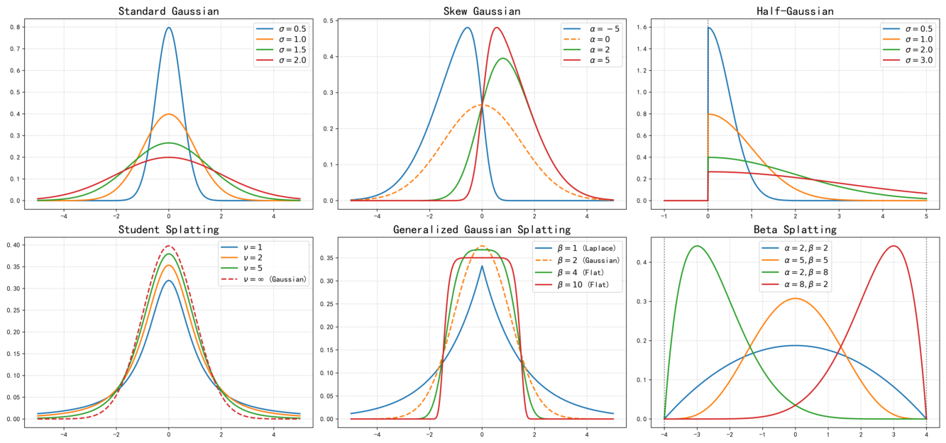
Figure 6.
Gaussian tile allocation by method. (a) 3D Gaussian Splatting allocates a Gaussian to a tile when that tile intersects the square inscribing the circle with radius defined. (b) Speedysplat’s SnugBox method allocates a Gaussian to a tile when that tile intersects the tight bounding box defined by the axis-aligned minima and maxima of the ellipse. (c) Speedysplat’s AccuTile method allocates a Gaussian to a tile only if that tile intersects the ellipse by algorithm, which computes the minimum and maximum tiles by iterating over the shorter side of the rectangular tile extent given by SnugBox. In this example, AccuTile algorithm iterates over the tile rows; the only points that are processed are and .
Figure 6.
Gaussian tile allocation by method. (a) 3D Gaussian Splatting allocates a Gaussian to a tile when that tile intersects the square inscribing the circle with radius defined. (b) Speedysplat’s SnugBox method allocates a Gaussian to a tile when that tile intersects the tight bounding box defined by the axis-aligned minima and maxima of the ellipse. (c) Speedysplat’s AccuTile method allocates a Gaussian to a tile only if that tile intersects the ellipse by algorithm, which computes the minimum and maximum tiles by iterating over the shorter side of the rectangular tile extent given by SnugBox. In this example, AccuTile algorithm iterates over the tile rows; the only points that are processed are and .
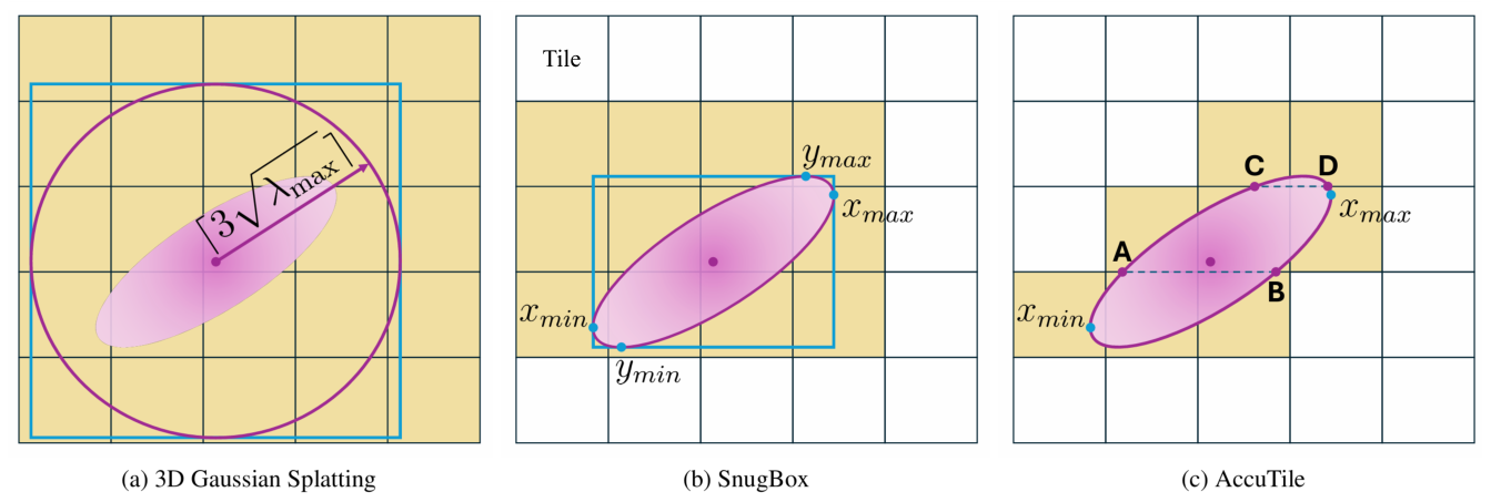
Figure 7.
Volumetrically consistent Computation. Top row: 3D Gaussians that are not grey contribute to the pixel along the camera ray. Next, 1D Gaussian densities along the ray are used to compute values required for color computation. Vol3DGS performs volumetrically consistent computation by accumulating the density along the ray in accordance with the volume rendering equation.
Figure 7.
Volumetrically consistent Computation. Top row: 3D Gaussians that are not grey contribute to the pixel along the camera ray. Next, 1D Gaussian densities along the ray are used to compute values required for color computation. Vol3DGS performs volumetrically consistent computation by accumulating the density along the ray in accordance with the volume rendering equation.
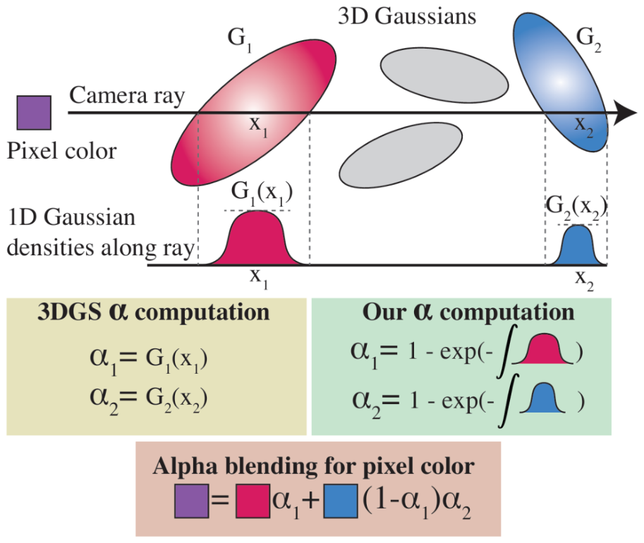
Figure 10.
Empirical Analysis of Gaussian Compression vs. Rendering Quality. Comparison of Gaussian count compression ratios (bar charts, left y-axis) and the corresponding variations relative to the 3DGS baseline (line plots, right y-axis) across Mip-NeRF 360, Tanks & Temples, and Deep Blending datasets. Traditionally, heavy compression incurs a noticeable penalty in visual fidelity (e.g., LightGaussian). However, recent state-of-the-art frameworks (e.g., MMGS and DashGaussian) successfully break this trade-off. By strategically culling redundant primitives or utilizing structural regularization, these methods achieve extreme compression ratios (often exceeding ) while simultaneously yielding a positive . This counter-intuitive quality improvement suggests that rigorous simplification not only reduces memory footprint but also inherently acts as a geometric regularizer, effectively suppressing high-frequency artifacts and "floaters" present in the baseline.
Figure 10.
Empirical Analysis of Gaussian Compression vs. Rendering Quality. Comparison of Gaussian count compression ratios (bar charts, left y-axis) and the corresponding variations relative to the 3DGS baseline (line plots, right y-axis) across Mip-NeRF 360, Tanks & Temples, and Deep Blending datasets. Traditionally, heavy compression incurs a noticeable penalty in visual fidelity (e.g., LightGaussian). However, recent state-of-the-art frameworks (e.g., MMGS and DashGaussian) successfully break this trade-off. By strategically culling redundant primitives or utilizing structural regularization, these methods achieve extreme compression ratios (often exceeding ) while simultaneously yielding a positive . This counter-intuitive quality improvement suggests that rigorous simplification not only reduces memory footprint but also inherently acts as a geometric regularizer, effectively suppressing high-frequency artifacts and "floaters" present in the baseline.
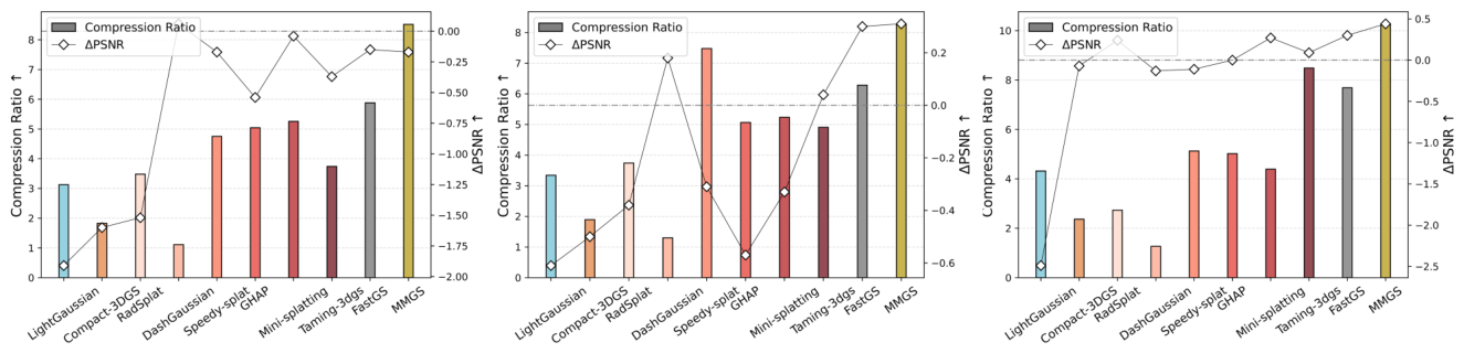
Figure 11.
Trade-off Dynamics between Training Efficiency and Rendering Fidelity. Plotting training time (logarithmic scale) against PSNR across three benchmark datasets. The baseline 3DGS typically requires substantial optimization time (clustering on the right). Modern algorithmic interventions aggressively push the Pareto frontier towards the top-left corner. Notably, methods such as MMGS and FastGS achieve an order-of-magnitude acceleration in convergence speed ( minutes) without sacrificing visual quality. This dramatic shift highlights the critical importance of hardware-aware thread scheduling, optimized densification strategies, and efficient visibility sorting over naive brute-force optimization.
Figure 11.
Trade-off Dynamics between Training Efficiency and Rendering Fidelity. Plotting training time (logarithmic scale) against PSNR across three benchmark datasets. The baseline 3DGS typically requires substantial optimization time (clustering on the right). Modern algorithmic interventions aggressively push the Pareto frontier towards the top-left corner. Notably, methods such as MMGS and FastGS achieve an order-of-magnitude acceleration in convergence speed ( minutes) without sacrificing visual quality. This dramatic shift highlights the critical importance of hardware-aware thread scheduling, optimized densification strategies, and efficient visibility sorting over naive brute-force optimization.
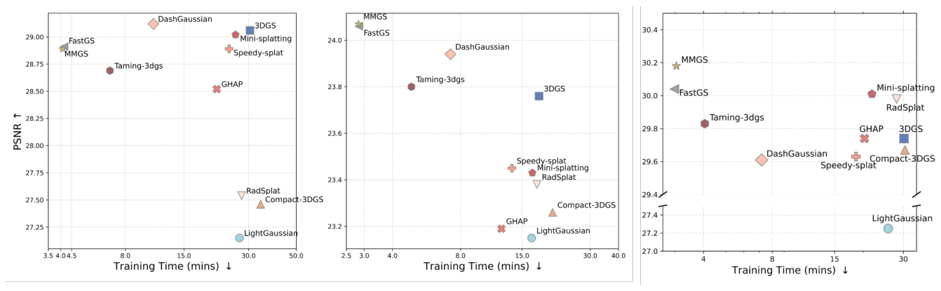
Figure 12.
Geometric Sparsity vs. Reconstruction Fidelity. Evaluation of the number of Gaussians (logarithmic scale) required to achieve specific PSNR levels. The baseline 3DGS is highly over-parameterized, often relying on millions of unstructured primitives to construct a scene. The distribution reveals that aggressive pruning and merging techniques can successfully cull over of the initial Gaussian population with minimal fidelity degradation. The emergence of highly sparse representations in the top-left quadrant empirically proves that complex 3D scenes exhibit significant low-rank or structural redundancies that can be exploited for highly compact explicit rendering.
Figure 12.
Geometric Sparsity vs. Reconstruction Fidelity. Evaluation of the number of Gaussians (logarithmic scale) required to achieve specific PSNR levels. The baseline 3DGS is highly over-parameterized, often relying on millions of unstructured primitives to construct a scene. The distribution reveals that aggressive pruning and merging techniques can successfully cull over of the initial Gaussian population with minimal fidelity degradation. The emergence of highly sparse representations in the top-left quadrant empirically proves that complex 3D scenes exhibit significant low-rank or structural redundancies that can be exploited for highly compact explicit rendering.
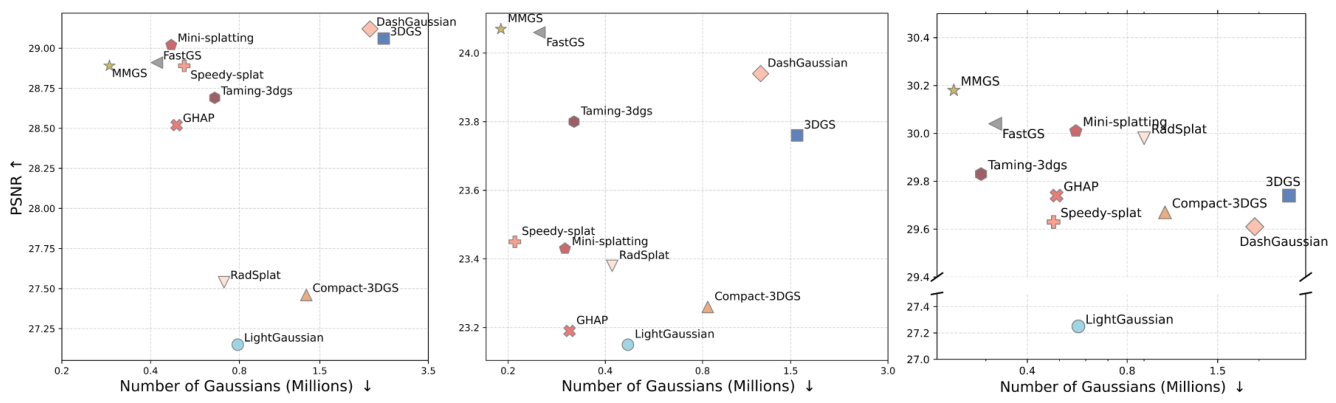
Figure 13.
Rate-Distortion Frontiers for Large-Scale Scene Compression. Storage size (MB, log scale) versus PSNR across unbounded environments from the Mip-NeRF 360, MatrixCity, and Tanks & Temples datasets. Unlike the vanilla 3DGS, advanced representations (such as PyramidGS, ContextGS, and HAC++) provide continuous rate-distortion curves via LoD or hierarchical quantization mechanisms. The massive reduction factors depicted demonstrate the transition of Gaussian splatting from memory-bound theoretical models to scalable assets suitable for resource-constrained edge deployment.
Figure 13.
Rate-Distortion Frontiers for Large-Scale Scene Compression. Storage size (MB, log scale) versus PSNR across unbounded environments from the Mip-NeRF 360, MatrixCity, and Tanks & Temples datasets. Unlike the vanilla 3DGS, advanced representations (such as PyramidGS, ContextGS, and HAC++) provide continuous rate-distortion curves via LoD or hierarchical quantization mechanisms. The massive reduction factors depicted demonstrate the transition of Gaussian splatting from memory-bound theoretical models to scalable assets suitable for resource-constrained edge deployment.
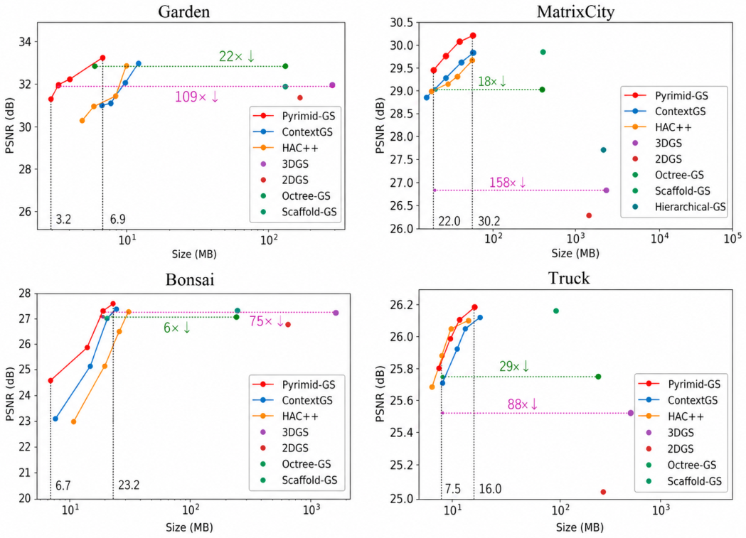
Table 2.
Quantitative Evaluation and Algorithmic Taxonomy across Benchmark Datasets. All evaluations adhere to the original 3DGS experimental protocols on the Mip-NeRF 360, Tanks & Temples, and Deep Blending datasets. The evaluated frameworks are structurally categorized into four distinct tiers: Tier 1 (Kernel Representations), Tier 2 (Sparsity & Acceleration), Tier 3 (Optimization Mechanisms), Tier 4 (LoD & Storage Compression). For all methods, we conducted experiments using our unified 3D Gaussian Splatting rasterization implementation for fair comparison.
Table 2.
Quantitative Evaluation and Algorithmic Taxonomy across Benchmark Datasets. All evaluations adhere to the original 3DGS experimental protocols on the Mip-NeRF 360, Tanks & Temples, and Deep Blending datasets. The evaluated frameworks are structurally categorized into four distinct tiers: Tier 1 (Kernel Representations), Tier 2 (Sparsity & Acceleration), Tier 3 (Optimization Mechanisms), Tier 4 (LoD & Storage Compression). For all methods, we conducted experiments using our unified 3D Gaussian Splatting rasterization implementation for fair comparison.
| Method | Publication | Mip-NeRF 360 | Tanks & Temples | Deep Blending | ||||||
|---|---|---|---|---|---|---|---|---|---|---|
| PSNR↑ | SSIM↑ | LPIPS↓ | PSNR↑ | SSIM↑ | LPIPS↓ | PSNR↑ | SSIM↑ | LPIPS↓ | ||
| 3DGS [8] | SIGGRAPH 2023 | 29.05 | 0.870 | 0.184 | 23.69 | 0.844 | 0.178 | 29.74 | 0.903 | 0.250 |
| 2DGS [64] | SIGGRAPH 2024 | 28.24 | 0.852 | 0.219 | 23.13 | 0.830 | 0.212 | 29.50 | 0.899 | 0.259 |
| 3DHGS [55] | CVPR 2025 | 29.47 | 0.871 | 0.179 | 24.35 | 0.857 | 0.169 | 29.41 | 0.899 | 0.244 |
| 3DSGS [61] | ARXIV 2026 | 29.49 | 0.878 | 0.165 | 24.36 | 0.858 | 0.173 | 29.75 | 0.904 | 0.236 |
| 3DSSS [56] | CVPR 2025 | 29.48 | 0.881 | 0.164 | 24.37 | 0.861 | 0.161 | 29.98 | 0.906 | 0.247 |
| GES [54] | CVPR 2024 | 28.50 | 0.855 | 0.212 | 23.43 | 0.836 | 0.198 | 29.62 | 0.901 | 0.252 |
| 3D Convex Splatting [57] | CVPR 2025 | 28.99 | 0.863 | 0.175 | 23.89 | 0.849 | 0.157 | 29.68 | 0.901 | 0.235 |
| BetaSplatting [58] | SIGGRAPH 2025 | 29.55 | 0.874 | 0.185 | 24.46 | 0.866 | 0.152 | 29.19 | 0.904 | 0.252 |
| LightGaussian [83] | NeurIPS 2024 | 28.47 | 0.858 | 0.212 | 23.03 | 0.816 | 0.232 | 27.23 | 0.874 | 0.298 |
| Mini-splatting [81] | ECCV 2024 | 29.02 | 0.869 | 0.170 | 23.43 | 0.844 | 0.181 | 30.01 | 0.907 | 0.243 |
| Speedy-splat [85] | CVPR 2025 | 28.89 | 0.869 | 0.198 | 23.45 | 0.820 | 0.240 | 29.63 | 0.905 | 0.256 |
| Taming-3dgs [82] | SIGGRAPH Asia 2024 | 28.69 | 0.852 | 0.223 | 23.80 | 0.833 | 0.212 | 29.83 | 0.899 | 0.274 |
| GHAP [201] | NeurIPS 2025 | 28.52 | 0.856 | 0.219 | 23.19 | 0.828 | 0.217 | 29.74 | 0.902 | 0.255 |
| DashGaussian [202] | CVPR 2025 | 29.12 | 0.872 | 0.186 | 23.94 | 0.847 | 0.181 | 29.61 | 0.902 | 0.249 |
| FastGS [88] | CVPR 2026 | 28.91 | 0.864 | 0.207 | 24.06 | 0.835 | 0.212 | 30.04 | 0.904 | 0.257 |
| MMGS [89] | ARXIV 2026 | 28.89 | 0.861 | 0.215 | 24.07 | 0.838 | 0.208 | 30.18 | 0.905 | 0.260 |
| GOF [63] | SIGGRAPH Asia 2024 | 28.74 | 0.874 | 0.177 | 23.60 | 0.854 | 0.167 | 28.87 | 0.879 | 0.278 |
| PGSR [65] | TVCG 2024 | 28.56 | 0.876 | 0.172 | 23.16 | 0.853 | 0.194 | 28.56 | 0.866 | 0.285 |
| Mip-Splatting [52] | CVPR 2024 | 29.31 | 0.880 | 0.168 | 23.83 | 0.852 | 0.175 | 29.35 | 0.903 | 0.244 |
| 3DGS-MCMC [75] | NeurIPS 2024 | 29.33 | 0.883 | 0.169 | 24.10 | 0.858 | 0.156 | 29.53 | 0.898 | 0.247 |
| Scaffold-GS [141] | CVPR 2024 | 29.35 | 0.870 | 0.188 | 23.96 | 0.853 | 0.177 | 30.21 | 0.906 | 0.254 |
| Octree-GS [142] | TPAMI 2025 | 29.11 | 0.867 | 0.188 | 24.68 | 0.866 | 0.153 | 29.65 | 0.901 | 0.257 |
| Wavelet-GS [155] | ACM MM 2025 | 29.68 | 0.870 | 0.170 | 24.40 | 0.863 | 0.124 | 30.38 | 0.909 | 0.231 |
| Compact-3DGS [203] | CVPR 2024 | 28.45 | 0.854 | 0.210 | 23.32 | 0.831 | 0.201 | 29.63 | 0.901 | 0.257 |
| ContextGS [160] | NeurIPS 2024 | 29.15 | 0.861 | 0.201 | 24.20 | 0.852 | 0.184 | 30.11 | 0.907 | 0.265 |
| HAC++ [162] | TPAMI 2025 | 29.26 | 0.865 | 0.207 | 24.32 | 0.854 | 0.178 | 30.16 | 0.907 | 0.266 |
| RadSplat [91] | ECCV 2024 | 27.54 | 0.825 | 0.239 | 23.38 | 0.831 | 0.208 | 29.98 | 0.908 | 0.255 |
Disclaimer/Publisher’s Note: The statements, opinions and data contained in all publications are solely those of the individual author(s) and contributor(s) and not of MDPI and/or the editor(s). MDPI and/or the editor(s) disclaim responsibility for any injury to people or property resulting from any ideas, methods, instructions or products referred to in the content. |
© 2026 by the authors. Licensee MDPI, Basel, Switzerland. This article is an open access article distributed under the terms and conditions of the Creative Commons Attribution (CC BY) license (http://creativecommons.org/licenses/by/4.0/).
Copyright: This open access article is published under a Creative Commons CC BY 4.0 license, which permit the free download, distribution, and reuse, provided that the author and preprint are cited in any reuse.


