

Submitted:
09 July 2026
Posted:
10 July 2026
You are already at the latest version
Abstract
Spatial self-organized patterns are ubiquitous features of vegetation ecosystems, and cyclic nontransitive competition serves as a crucial intrinsic mechanism for sustaining biodiversity. However, existing studies lack cross-scale comparative analyses of vegetation territorial competition based on multiple models. This study combines lattice models and continuous differential equation models to investigate the territorial occupation dynamics and spatial evolution of vegetation communities driven by cyclic competition. The results demonstrate that cyclic competition acts as a core mechanism maintaining vegetation biodiversity, which enables the self-organization of stable spiral wave patterns in space and supports the long-term dynamic coexistence of multiple species. Discrete and continuous models exhibit highly consistent macroscopic dynamical behaviors, which reveal the intrinsic dynamical characteristics of cyclic competitive systems. By integrating microscopic lattice simulation and macroscopic differential equation analysis, this study verifies that spiral waves represent a highly robust species coexistence mode and clarifies the coupled regulatory effects of species richness and stochasticity on system evolution. The findings further deepen the understanding of the complexity of vegetation ecosystems and provide important theoretical references for subsequent theoretical derivation and field observational research on vegetation community competition and evolution.
Keywords:
cyclic competition
; lattice model
; spiral wave
; species coexistence
MSC: [2010] 35B36; 35C07; 35G50
1. Introduction
Spatial pattern formation is a ubiquitous natural phenomenon across scales, ranging from macroscopic ecosystems to microscopic cellular tissues [1]. In ecology, unraveling the mechanisms underlying such spatial patterns is critical for addressing core research questions including species coexistence, community stability, and ecosystem functioning. For instance, vegetation in arid and semi-arid regions frequently develops regular geometric configurations such as patches, stripes, or labyrinths [2,3], and the emergence of these patterns is generally attributed to scale-dependent feedback mechanisms [1,4]. In recent years, researchers have incorporated additional complex factors into relevant investigations, such as nonlocal interactions [5], fractional-order dynamics [6], and community succession under climate change scenarios [7], which have substantially advanced our understanding of the formative mechanisms of vegetation spatial patterns.
Beyond the interactions between vegetation and environmental resources, direct interspecific competition acts as a vital driving force shaping community structure and spatial distribution [8]. Classical competition theories predominantly focus on hierarchical competition, where species are ordered by clear dominance hierarchies. Nevertheless, natural ecosystems harbor a more complex form of intransitive competitive interaction, commonly referred to as cyclic competition [9]. Cyclic competition prevails extensively across real ecological systems. For example, in certain populations of side-blotched lizards, male individuals engage in cyclic competition via three distinct throat-color strategies: aggressive, defensive, and sneaker tactics [10]. Within microbial communities, different strains of E. coli establish cyclic competitive relationships through toxin production, resistance, and susceptibility, which in turn sustains strain diversity [11]. Analogous phenomena have also been documented among marine sessile organisms and plant communities [9]. The core ecological implication of cyclic competition lies in its role as a powerful mechanism for the maintenance of biodiversity.
To investigate the spatial dynamics of cyclic competition systems, researchers have developed a variety of modeling approaches. Among them, Individual-Based Models (IBMs), especially lattice models, represent the most widely adopted category [12]. In lattice models, space is discretized into a grid, with each lattice site corresponding to a habitat occupied by an individual of a single species. Interactions among individuals (e.g., competition, reproduction, dispersal) follow a set of predefined stochastic rules [13,14]. The strength of such models lies in their ability to intuitively capture critical microscopic features including stochastic fluctuations, individual discreteness and local interactions, making them well-suited for investigating complex spatiotemporal dynamics via computer simulations [15,16]. Nevertheless, lattice models also carry limitations: the generality of their outputs can be sensitive to detailed settings such as lattice geometry and neighborhood definition, and rigorous mathematical analysis is difficult to implement. Contrasting with lattice models are macroscopic continuous-field models, which are generally formulated by a system of differential equations [17]. The major advantage of differential equation models stems from their robust mathematical analytical capacity. Tools such as stability analysis and bifurcation theory can be adopted to precisely predict macroscopic properties including the threshold conditions for pattern formation, wave propagation speed and wavelength [18]. However, the derivation of differential equation models commonly neglects individual discreteness and stochastic fluctuations, which may prevent these models from fully reproducing certain noise-induced phenomena.
Bridging microscopic lattice models and macroscopic differential equation models constitutes a core challenge and vital research frontier in theoretical ecology [19]. Constructing a linkage between these two types of models not only provides solid theoretical interpretations for simulation outputs from lattice models, but also endows parameters of PDE models with explicit micro-biological interpretations. Such cross-scale research approaches enable a more comprehensive and in-depth understanding of the dynamical behaviors of ecological systems [20,21].
Although numerous existing studies have separately explored vegetation spatial patterns [22] and interspecific cyclic competition [23,24], few studies have developed and compared discrete lattice models and continuous differential equation models for vegetation territorial competition, and cross-scale integrated analyses are still lacking. Against this backdrop, this study adopts multi-species vegetation communities with cyclic competition as the research object. We construct a microscopic two-dimensional stochastic lattice model and a macroscopic continuous dynamic model respectively. By integrating numerical simulations and stability analysis, we investigate how species richness and environmental noise modulate vegetation spatial patterns and population coexistence dynamics, reveal the core mechanism by which cyclic competition generates self-organized spiral wave patterns and preserves vegetation diversity, and establish a unified theoretical framework linking microscopic individual interactions and macroscopic community evolution.
2. Methods
2.1. 2 Dimensional (2D) Lattice Model
Simulations are performed on a two-dimensional grid, and periodic boundary conditions are implemented to eliminate boundary effects. Each lattice site is occupied by only one single vegetation species. At the initial time step, vegetation species are randomly assigned to all lattice sites with equal probability. The model rules are illustrated using a system with vegetation species as an example (Figure 1). In subplot (a), arrows point from competitively dominant vegetation to inferior vegetation, forming a closed loop. Subplot (b) demonstrates the update rules for a single lattice site. Take vegetation 3 located at the center of a Moore neighborhood at time t as an example. Let C denote the number of neighboring vegetation 2 individuals surrounding the central vegetation 3. We define , where represents uniform white noise with a mean of 0 and variance of , and is the noise intensity parameter. If and is greater than or equal to the threshold , the central vegetation 3 will be replaced by vegetation 2 at time .
2.2. Differential Equation Model
The dynamic equation governing the population density of each vegetation species is established based on cyclic interspecific competition and resource occupation mechanisms. Within this closed cyclic competition framework, every species undergoes two distinct competitive influences from its adjacent counterparts in the ecological loop.
The first term functions as the population gain term for species i. From an ecological perspective, species i regards species as its target for resource occupation. A higher population abundance of lives space and essential limiting resources (including light, moisture and soil nutrients) for the reproduction and expansion of species i, and accordingly delivers a positive, boosting contribution to the growth rate of .
In comparison, the second term represents the population loss term. Species is a direct invasive competitor of species i: it continuously seizes the finite survival resources required by species i and squeezes its viable habitat. Such unilateral resource occupation imposes a strong inhibitory constraint on the population growth of species i, driving the decline of its population density and generating a persistent negative loss effect on the temporal evolution of .
Combining these two counteracting competitive contributions, we arrive at the dynamical relation
where denotes the population density of the i-th vegetation species, and the non-zero constant c represents the uniform interspecific competition strength among vegetation populations.
To close the cyclic competitive chain for vegetation species, periodic boundary conditions and are imposed to resolve the out-of-bound subscripts at the two ends of the species sequence. Here, the non-zero constant c uniformly quantifies the overall strength of interspecific resource competition and occupation; the absolute value governs the magnitude of population fluctuations induced by cyclic interactions, while the sign of c only reverses the rotational direction of periodic population oscillations without altering the inherent competitive topology of the system. This mean-field model applies to small spatial domains where spatial heterogeneity and dispersal gradients can be safely neglected.
For large spatial domains where spatial heterogeneity cannot be ignored, the spatial characteristics of the system must be taken into account. Equation (1) is rewritten as
where D denotes the diffusion coefficient shared by all vegetation species, and is . Numerical simulations for this model are implemented on a grid with periodic boundary conditions.
Numerical computations commenced with spatial discretization of the partial differential equation (PDE) system outlined in Eq. (2) via the nine-point finite difference scheme. This spatial transformation converted the coupled PDE set into a system of ordinary differential equations (ODEs). Afterwards, the derived ODE formulations and Eq. (1) were numerically integrated with the fourth-order Runge-Kutta algorithm, adopting a fixed time increment of . The parameter c is , and the scaled diffusion coefficient is 0.1 (h is the spatial step).
3. Results
3.1. Results of the Lattice Model
We first investigate the scenario with three vegetation species, and Figure 2 illustrates the evolutionary process of vegetation spatial distribution within the system under the parameter . The system evolves from an initial random distribution into dynamically stable spiral wave patterns, and the spatial distribution of vegetation exhibits obvious regularity and stratification. Throughout the entire evolution process, no phenomenon occurs in which a single dominant vegetation species expands excessively or inferior species go completely extinct. The system eventually forms large-scale stable patch structures and realizes dynamic balanced coexistence of multiple vegetation species. The maintenance of this steady state stems from the persistent existence of spiral wave cores. The cyclic competitive relationships remain stable without evident attenuation, thereby guaranteeing long-term coexistence of the three-species vegetation system.
To accurately reflect the quantitative variation of each vegetation species within the system, we calculate the population density of each vegetation species, defined as the proportion of lattice sites occupied by the corresponding species, i.e., the ratio between the number of lattice sites occupied by one vegetation species and the total number of lattice sites. Figure 3 depicts the temporal evolution of population density for all vegetation species. The population density of each species oscillates around the value of , demonstrating the characteristic of dynamic equilibrium.
x
Next, we increase the number of vegetation species to examine the effect of species number N on vegetation spatial patterns. Figure 4 presents the evolutionary processes of spatial patterns for systems containing 4 to 7 vegetation species with the parameter . The results reveal that for and , spiral wave structures can still emerge spontaneously among vegetation species, and the system eventually reaches dynamic equilibrium. In contrast, when and , the spatial distribution of vegetation retains the initial random configuration and presents static patterns.
Figure 5 illustrates the temporal evolution of vegetation population density for each system shown in Figure 4. For systems with and , the population density of each species oscillates around , exhibiting dynamic equilibrium. By contrast, when and , the population density of each vegetation species remains at its initial value of without any fluctuations.
The fundamental reason for the loss of dynamical evolution in systems with and is that the total number C of competitively dominant neighboring vegetation individuals around each lattice site declines as N rises, such that cannot exceed the threshold . Accordingly, the system can be restored to dynamic equilibrium by raising the noise intensity or lowering the threshold . Figure 6 displays the evolution of vegetation patterns for systems with six and seven vegetation species under , where the systems eventually evolve into dynamically balanced spatiotemporal spiral wave patterns. This demonstrates that elevating noise intensity is capable of recovering the system’s dynamical equilibrium. In addition, as N increases, the contiguous spatial domains occupied by a single vegetation species within spiral waves expand.
To gain a more detailed insight into the system behaviors, we investigate system states across the parameter plane. Figure 7 presents the probability that the system exhibits dynamic equilibrium within this parameter plane. These results indicate that higher noise intensity is required to restore the system’s dynamic equilibrium as N increases, which is consistent with the above conjecture.
3.2. Results of the Differential Equation Model
When spatial heterogeneity is negligible, Eq. (1) can characterize the temporal evolution of population density for each vegetation species within the system. Figure 8 separately illustrates the evolutionary trajectories of population density for each vegetation species under . The results show that all vegetation species restrict one another mutually; no single species undergoes sustained population expansion or decline. The population density of each species undergoes persistent oscillations around , and no vegetation species goes extinct throughout the evolution process. These findings are consistent with the dynamic coexistence features of multiple vegetation species observed in the lattice model. Theoretically, this outcome demonstrates that cyclic competition systems can sustain long-term community stability and verifies the inherent rationality of this mechanism for supporting multi-species coexistence.
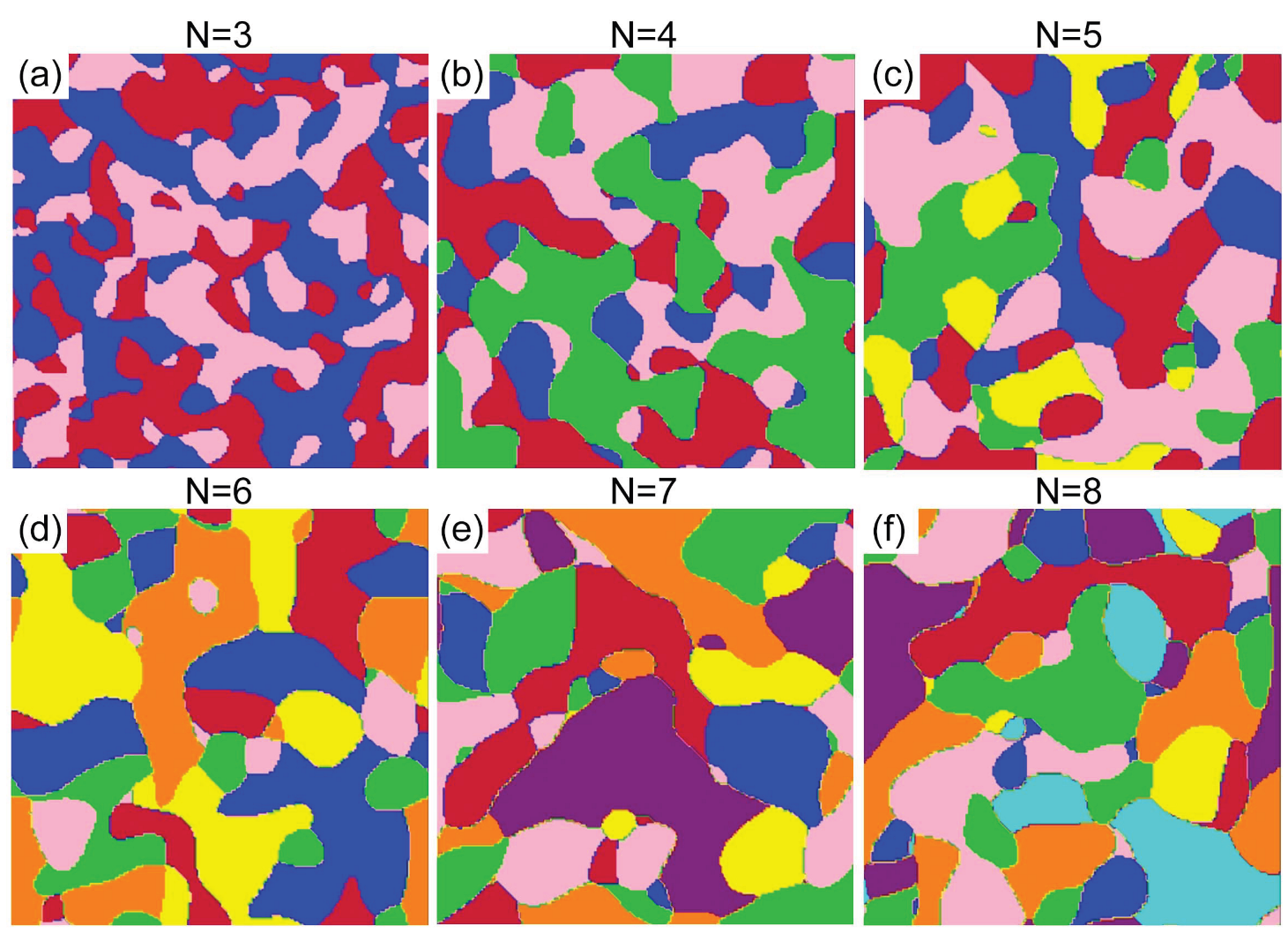
For systems with extensive spatial domains where spatial heterogeneity is non-negligible, Eq. (2) governs the spatiotemporal evolution of spatial patterns for all vegetation species in the community. We derive the corresponding vegetation spatial patterns for based on Eq. (2), as presented in Figure 9. The results reveal that dynamic spiral wave patterns ultimately emerge in all systems. Specifically, the habitat ranges of each vegetation species migrate back and forth around fixed points, demonstrating dynamic coexistence equilibrium. These outcomes are consistent with those obtained from the lattice model.
4. Analytical Results
4.1. Conservation of Total Quantity
Summing all equations in Eq. (1) yields
Therefore, the total vegetation biomass of the system satisfies conservation, namely,
where is a constant determined by the initial conditions.
4.2. Linear Stability Analysis
Setting the time derivative of population density to zero yields the criterion for fixed points of the system:
Solving Eq. (5) together with Eq. (4) allows the non-trivial fixed points to be classified into three categories: single-species survival, coexistence of partial vegetation species, and coexistence of all vegetation species.
We next conduct separate analyses taking the cases of and as examples. We construct the fixed-point equations corresponding to , i.e.,
When the population density of certain vegetation species equals zero, this corresponds to the survival of a single species and the extinction of the remaining species. Three sets of fixed points are obtained: , , and . The Jacobian matrix of the system is denoted as
Substituting yields
The characteristic equation is given by
Solving it gives the eigenvalues , so is an unstable saddle point. Similarly, it can be proven that and are also unstable saddle points. This indicates that the state where a single species dominates the community cannot resist tiny perturbations and cannot persist over the long term.
When the population densities of all three vegetation species are positive, combining the equilibrium condition (6), we can derive that . Substituting this into the total conservation equation (4), the coexistence fixed point is solved as . The corresponding characteristic equation can be obtained: . The solved eigenvalues are , where . Since the eigenvalues contain a zero root and a pair of conjugate purely imaginary roots, is a neutral fixed point.
The fixed-point equations corresponding to four vegetation species are as follows:
When only one vegetation species survives in the community and all other species go extinct, there exist four such fixed points, which are respectively given by
The stability analysis is carried out taking the fixed point as an example. The Jacobian matrix of the system is
Substituting the fixed point yields the characteristic equation
The solved eigenvalues are . Hence, is an unstable saddle point. Similarly, it can be verified that , and are also unstable saddle points.
When vegetation species survive alternately, set . By combining the total mass conservation constraint , we obtain the first family of fixed points . The solved eigenvalues are . If , the eigenvalues include one positive and one negative real root, so the fixed point is an unstable saddle point. If , the fixed point is a neutral fixed point. For the alternate survival case with , it can be proven that the stability of the corresponding fixed point is consistent with the above result.
For the coexisting equilibrium of the four vegetation species, the constraint relations and can be derived from the equilibrium condition Eq. (8). Let and . Substitute them into the total conservation equation Eq. (4) and simplify to obtain . Accordingly, the family of coexistence fixed points reads . The eigenvalues are solved as . The system possesses two zero eigenvalues together with a pair of conjugate purely imaginary roots, which implies a degenerate critical state, and the fixed point is neutral.
4.3. Conservative Oscillations
We construct a multiplicative function . Taking the time derivative yields
Hence, V is a conserved quantity of the system whose value remains invariant over time. Combined with the total population conservation constraint , the trajectories of the system are confined within the N-dimensional phase space. In detail, all trajectories are restricted to the conserved subspace formed simultaneously by the hyperplane and the hypersurface (with constant K). As a result, the system undergoes persistent conservative oscillations along these closed orbits.
5. Conclusions and Discussions
This study constructs and analyzes lattice models and continuous differential equation models to investigate the territory occupation dynamics and spatial pattern formation mechanisms driven by cyclic competition within vegetation communities. The results verify that cyclic competition serves as a core functional mechanism sustaining vegetation biodiversity, which can self-organize to generate stable spiral wave patterns in space and enable long-term dynamic coexistence of multiple species. The macroscopic dynamical behaviors of the two types of models are highly consistent, collectively revealing the inherent dynamical characteristics of cyclic competitive systems. This research highlights the central role of spatial self-organization in biodiversity conservation. By unifying microscopic and macroscopic modeling frameworks, this work not only demonstrates that spiral waves constitute a highly robust coexistence regime for species, but also disentangles the complex coupling effects of species richness and stochasticity on system evolution. Our findings advance the understanding of ecosystem complexity and offer theoretical references for subsequent theoretical deductions and field observational investigations.
One of our core findings is that spiral waves, as stable spatiotemporal structures, play a pivotal role in sustaining species coexistence. In our simulations, spiral waves emerge from initial random distributions in both individual-based lattice models and population-density-based partial differential equation (PDE) models. The formation of such patterns is consistent with previous findings reported for other cyclic competitive systems [25,26]. The rotational cores of spiral waves function as dynamic refuges, preventing any single species from being completely eliminated by its competitively superior counterparts. This breaks the cyclic species extinctions commonly observed in non-spatial models and stabilizes the entire community [11]. Our results offer a novel perspective for interpreting vegetation pattern formation in natural ecosystems [27,28], distinct from the classical scale-dependent feedback mechanism [29,30]: direct non-transitive interactions among species alone are sufficient to trigger large-scale spatial self-organization.
Another important contribution of this study lies in the successful linkage between the microscopic stochastic lattice model and the macroscopic deterministic differential equation model. The lattice model is capable of capturing key microscopic features such as individual discreteness and stochastic fluctuations. One particularly intriguing finding concerns the constructive effect of noise within the lattice model: systems with a larger number of species become trapped in frozen static patterns under low noise levels, whereas elevating noise intensity can reactivate the system and restore the dynamically coexisting spiral wave states. This indicates that environmental stochastic perturbations or intrinsic demographic randomness may not act as disruptive forces in complex communities with abundant species; instead, they constitute an essential prerequisite for sustaining system dynamics and species coexistence. In contrast, the deterministic PDE model fails to capture such noise-induced phase transitions, yet it excels in rigorous mathematical analysis. Our linear stability analysis and derivations of conserved quantities lay a solid theoretical foundation for understanding why the system tends to undergo persistent oscillations around coexistence fixed points, and further explain the instability of single-species dominance states. The mutual consistency of results obtained from the two models not only strengthens the reliability of our conclusions but also demonstrates the great potential of cross-scale modeling in ecological research [21].
Our research further reveals the profound influence of species richness (N) on system dynamics. In both models, the wavelength of spiral waves and the size of patches increase with rising N. Nevertheless, sustaining dynamic coexistence becomes more challenging in lattice models, which requires higher noise intensity. This implies that growing species diversity in cyclically competing communities may come at the cost of greater reliance on stochasticity. This finding provides insights into disentangling the intricate relationship between biodiversity and ecosystem stability. When competitive networks grow more complex—for instance, those incorporating multiple competing cycles [31] or distinct coalition structures [14,15]—the resulting system dynamics can become far more diverse and less predictable.
Although our model successfully reproduces the key dynamical signatures of cyclic competition, we also recognize its inherent limitations. First, the model adopts substantial simplifications; for example, all species are assumed to possess identical competitive strength (c) and diffusion coefficient (D). In real vegetation communities, species exhibit pronounced disparities in growth, reproduction and dispersal capacity. The incorporation of asymmetric competitive rates [13,32] and species-specific mobility [33,34] may drastically alter the spatiotemporal dynamics and coexistence criteria of the system. Second, despite the functional effectiveness of the threshold-based replacement rule in the lattice model, its direct biological counterpart remains unclear, calling for future exploration of interaction mechanisms with stronger biological realism. Furthermore, our model omits numerous other vital ecological processes, including environmental heterogeneity, resource competition, natural disturbances [35], grazing [36], and long-term community succession [37].
Acknowledgments
This work is supported by the Action Program for Cultivating Young and Middle-Aged Faculty in Institutions of Higher Education under Grant no. YQZD2025055 (J. Gao), the National Natural Science Foundation of China under Grant no. 12205006 (J. Gao), and the Excellent Youth Scientific Research Project of Anhui Province under Grant no. 2022AH030107 (J. Gao).
References
- Borgogno, F.; D’odorico, P.; Laio, F.; Ridolfi, L. Mathematical models of vegetation pattern formation in ecohydrology. Rev. Geophys. 2009, 47(1), RG1005. [Google Scholar] [CrossRef]
- HilleRisLambers, R.; Rietkerk, M.; Van Den Bosch, F.; Prins, H. H. T.; de Kroon, H. Vegetation pattern formation in semi-arid grazing systems. Ecology 2001, 82(1), 50–61. [Google Scholar] [CrossRef]
- Gowda, K.; Riecke, H.; Silber, M. Transitions between patterned states in vegetation models for semiarid ecosystems. Phys. Rev. E 2014, 89(2), 022701. [Google Scholar] [CrossRef]
- Consolo, G.; Curro, C.; Grifo, G.; Valenti, G. Vegetation pattern formation and transition in dryland ecosystems with finite soil resources and inertia. Phys. D. 2025, 476, 134601. [Google Scholar] [CrossRef]
- Liu, L.; Maimaiti, Y. Spatiotemporal dynamics of nonlocal water-plant models: Insights into the mechanisms of vegetation pattern formation. Adv. Contin. Discret. M. 2025, 2025(1), 1–26. [Google Scholar] [CrossRef]
- Li, S.; Maimaiti, Y. Stability and bifurcation analysis of a time-order fractional model for water-plants: Implications for vegetation pattern formation. Math. Comput. Simulat. 2025, 234, 342–358. [Google Scholar] [CrossRef]
- Ferré, M. A.; Pavithran, I.; Bera, B. K.; Uecker, H.; Meron, E. Vegetation pattern formation and community assembly under drying climate trends. Chaos 2025, 35(9), 093114. [Google Scholar] [CrossRef] [PubMed]
- Durrett, R.; Levin, S. Spatial aspects of interspecific competition. Theor. Popul. Biol. 1998, 53(1), 30–43. [Google Scholar] [CrossRef] [PubMed]
- Szolnoki, A.; Mobilia, M.; Jiang, L. L.; Szczesny, B.; Rucklidge, A. M.; Perc, M. Cyclic dominance in evolutionary games: A review. J. R. Soc. Interface 2014, 11(100), 20140735. [Google Scholar] [CrossRef] [PubMed]
- Sato, K. Effects of cyclic allele dominance rules and spatial structure on the dynamics of cyclic competition models. Math. Biosci. Eng. 2020, 17(2), 1479–1494. [Google Scholar] [CrossRef]
- Laird, R. A. Population interaction structure and the coexistence of bacterial strains playing `rock–paper–scissors’. Oikos 2014, 123(4), 472–480. [Google Scholar] [CrossRef]
- Daly, A. J.; Quaghebeur, W.; Depraetere, T.; Baetens, J. M.; De Baets, B. Coexistence in three-species cyclic competition: Lattice-based versus lattice-free individual-based models. International Conference on Cellular Automata, 2018; Springer; pp. pages 115–124. [Google Scholar]
- He, Q.; Mobilia, M.; Täuber, U. C. Spatial rock-paper-scissors models with inhomogeneous reaction rates. Phys. Rev. E 2010, 82(5), 051909. [Google Scholar] [CrossRef]
- Szabó, G.; Szolnoki, A.; Borsos, I. Self-organizing patterns maintained by competing associations in a six-species predator-prey model. Phys. Rev. E 2008, 77, 041919. [Google Scholar] [CrossRef]
- Szabó, G. Competing associations in six-species predator–prey models. J. Phys. A Math. Gen. 2005, 38(30), 6689–6702. [Google Scholar] [CrossRef]
- Lütz, A. F.; Risau-Gusman, S.; Arenzon, J. J. Intransitivity and coexistence in four species cyclic games. J. Theor. Biol. 2013, 317, 286–292. [Google Scholar] [CrossRef] [PubMed]
- Manna, K.; Volpert, V.; Banerjee, M. Pattern formation in a three-species cyclic competition model. B. Math. Biol. 2021, 83(5), 52. [Google Scholar] [CrossRef]
- Ni, X.; Wang, W. X.; Lai, Y. C.; Grebogi, C. Cyclic competition of mobile species on continuous space: Pattern formation and coexistence. Phys. Rev. E 2010, 82(6), 066211. [Google Scholar] [CrossRef]
- Avelino, P. P.; de Oliveira, B. F.; Trintin, R. S. Lotka-Volterra versus May-Leonard formulations of the spatial stochastic rock-paper-scissors model: The missing link. Phys. Rev. E 2022, 105(2), 024309. [Google Scholar] [CrossRef] [PubMed]
- Strang, G. On the construction and comparison of difference schemes. SIAM J. Numer. Anal. 1968, 5(3), 506–517. [Google Scholar] [CrossRef]
- Karachalios, N. I.; Krypotos, A.; Kyriazopoulos, P. Nonlinear lattices from the physics of ecosystems: The Lefever–Lejeune nonlinear lattice in Z2. Math. Method. Appl. Sci. 2024, 47(16), 12487–12506. [Google Scholar] [CrossRef]
- Zhang, H.; Huang, T.; Dai, L.; Pan, G.; Liu, Z.; Gao, Z.; Zhang, X. Regular and irregular vegetation pattern formation in semiarid regions: A study on discrete Klausmeier model. Complexity 2020, 2020(1), 2498073. [Google Scholar] [CrossRef]
- He, Q.; Täuber, U. C.; Zia, R. K. P. On the relationship between cyclic and hierarchical three-species predator-prey systems and the two-species Lotka-Volterra model. Eur. Phys. J. B 2012, 85(4), 141. [Google Scholar] [CrossRef]
- Palombi, F.; Ferriani, S.; Toti, S. Coevolutionary dynamics of a variant of the cyclic Lotka–Volterra model with three-agent interactions. Eur. Phys. J. B 2020, 93(10), 194. [Google Scholar] [CrossRef]
- Reichenbach, T.; Mobilia, M.; Frey, E. Noise and correlations in a spatial population model with cyclic competition. Phys. Rev. Lett. 2007, 99(23), 238105. [Google Scholar] [CrossRef] [PubMed]
- Reichenbach, T.; Mobilia, M.; Frey, E. Self-organization of mobile populations in cyclic competition. J. Theor. Biol. 2008, 254(2), 368–383. [Google Scholar] [CrossRef] [PubMed]
- White, P. S. Pattern, process, and natural disturbance in vegetation. Bot. Rev. 1979, 45(3), 229–299. [Google Scholar] [CrossRef]
- Legendre, P.; Fortin, M. J. Spatial pattern and ecological analysis plant ecology; 1989. [Google Scholar]
- Klausmeier, C. A. Regular and irregular patterns in semiarid vegetation. Science 1999, 284(5421), 1826–1828. [Google Scholar] [CrossRef] [PubMed]
- Kéfi, S.; Rietkerk, M.; Alados, C.; Pueyo, Y.; Papanastasis, V. P.; ElAich, A.; De R., Peter C. Spatial vegetation patterns and imminent desertification in mediterranean arid ecosystems. Nature 2007, 449(7159), 213–217. [Google Scholar] [CrossRef] [PubMed]
- Noguchi, H. Dynamics due to competitive flip cycles in active potts models. Phys. Rev. E 2026, 113(3), 034210. [Google Scholar] [CrossRef] [PubMed]
- Pei, K.; Pei, Y.; Li, C. Effects of asymmetric rates and impulse interference in rock-paper-scissors games. Phys. D. 2024, 470, 134384. [Google Scholar] [CrossRef]
- Adamson, M. W.; Morozov, A. Y. Revising the role of species mobility in maintaining biodiversity in communities with cyclic competition. B. Math. Biol. 2012, 74(9), 2004–2031. [Google Scholar] [CrossRef]
- Mobilia, M.; Rucklidge, A. M.; Szczesny, B. The influence of mobility rate on spiral waves in spatial rock-paper-scissors games. Games 2016, 7(3), 24. [Google Scholar] [CrossRef]
- Wang, J.; Xie, X.; Li, W.; Chen, X.; Zhang, X.; Fan, N.; Wang, T.; Zhang, H. Damage-fracture evolution mechanism of rock bridge structures in flawed sandstone under cyclic disturbance: Insights from DIC-AE. Theor. Appl. Fract. Mec. 2010, 140, 21. [Google Scholar]
- Adler, P.; Raff, D.; Lauenroth, W. The effect of grazing on the spatial heterogeneity of vegetation. Oecologia 2001, 128(4), 465–479. [Google Scholar] [CrossRef] [PubMed]
- Kirkpatrick, J. B.; Gibson, N.; Fitzgerald, N. Stability among cyclic change in an Antipodean pond and bolster heath system 1983–2017. Aust. J. Bot. 2021, 69(8), 610–621. [Google Scholar] [CrossRef]
Figure 1.
Rules of the lattice model. (a) A cyclic competition system consisting of five vegetation species, where arrows point from competitively superior vegetation to inferior vegetation. (b) Vegetation replacement rules illustrated by the vegetation at the center of a grid. The left panel shows the spatial distribution at time t, and the right panel displays the distribution at time .
Figure 1.
Rules of the lattice model. (a) A cyclic competition system consisting of five vegetation species, where arrows point from competitively superior vegetation to inferior vegetation. (b) Vegetation replacement rules illustrated by the vegetation at the center of a grid. The left panel shows the spatial distribution at time t, and the right panel displays the distribution at time .
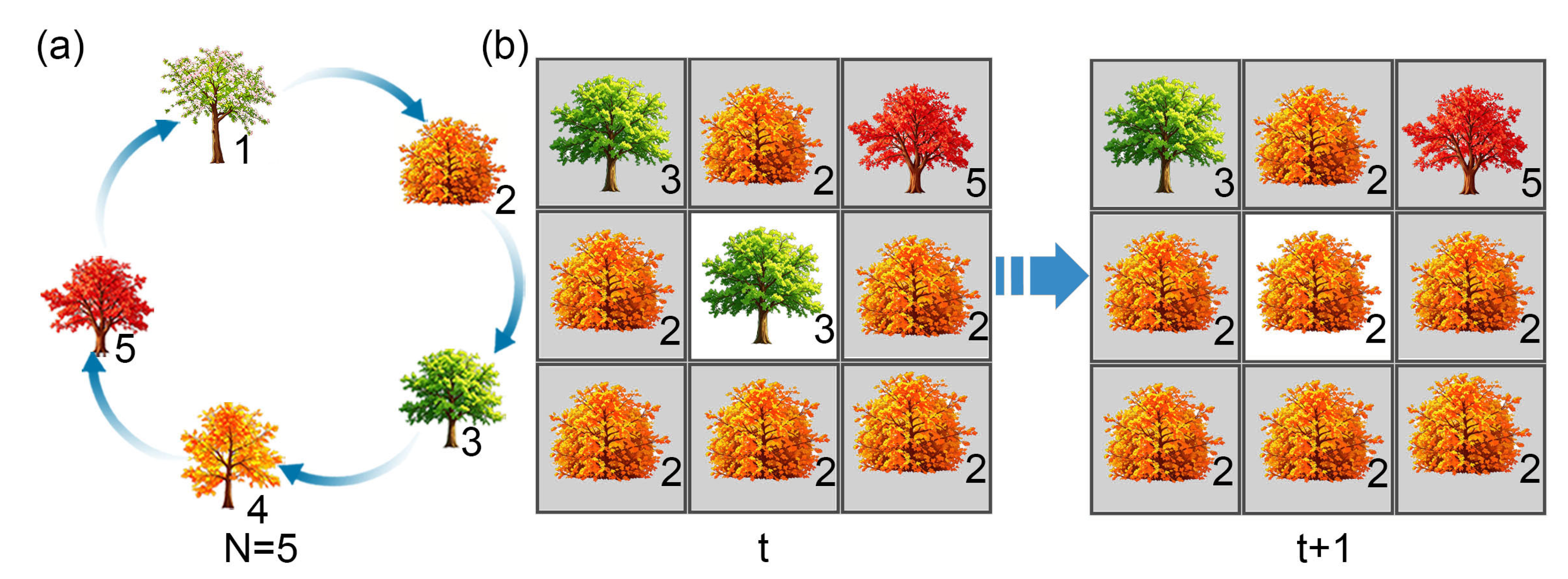
Figure 2.
Spatial pattern evolution of the three-species vegetation system at noise intensity . Red, dark blue, and pink represent vegetation species 1, 2, and 3, respectively. Panels (a-d) show snapshots of the system at generations , 2000, 12000, and 20000 in sequence.
Figure 2.
Spatial pattern evolution of the three-species vegetation system at noise intensity . Red, dark blue, and pink represent vegetation species 1, 2, and 3, respectively. Panels (a-d) show snapshots of the system at generations , 2000, 12000, and 20000 in sequence.
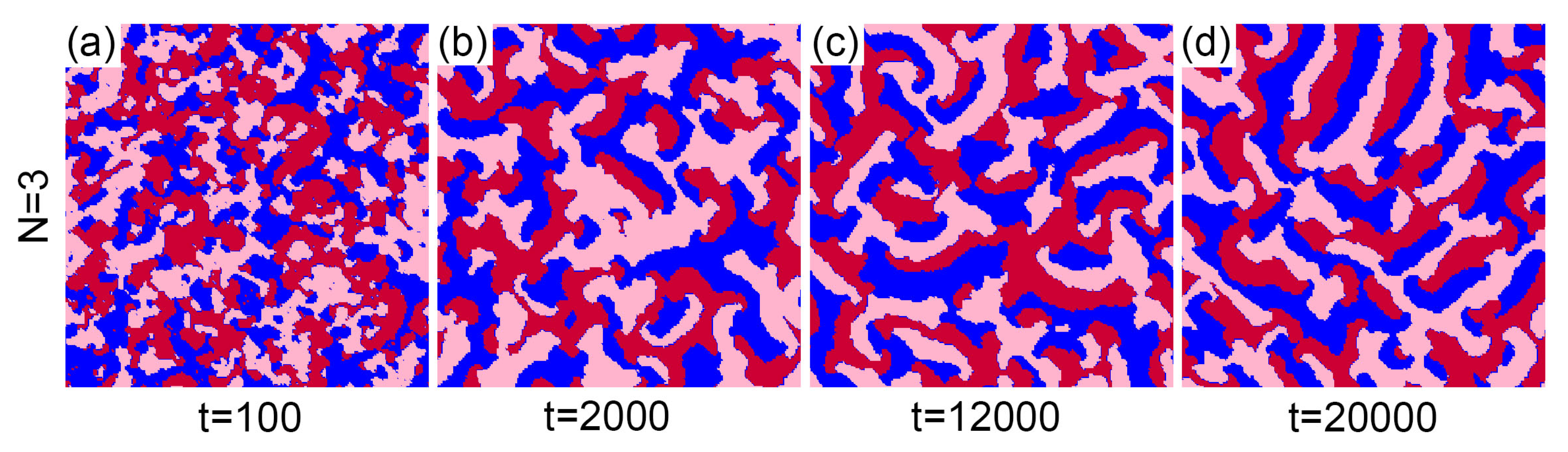
Figure 3.
Temporal evolution of population densities of each vegetation species in Figure 2.
Figure 3.
Temporal evolution of population densities of each vegetation species in Figure 2.
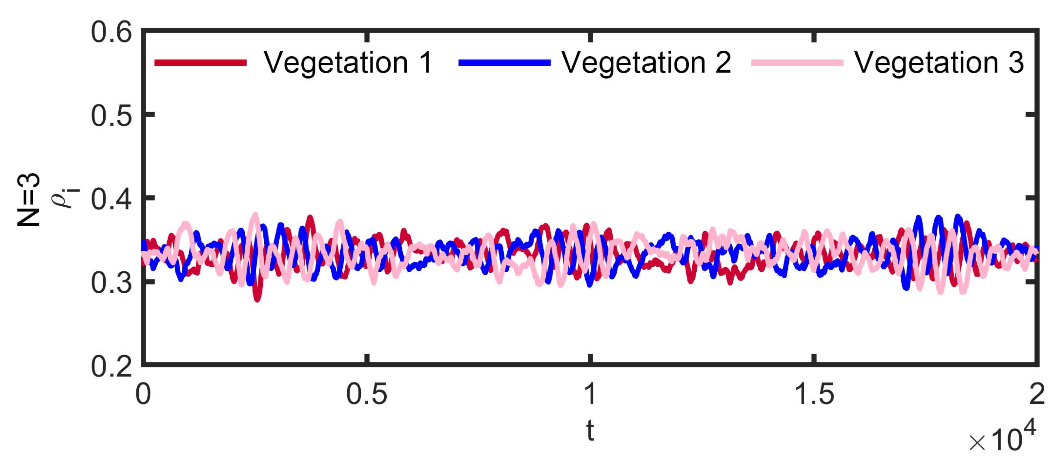
Figure 4.
Spatial pattern evolution of systems with more vegetation species under noise intensity . Panels (a)-(d) correspond to , respectively. From left to right in each column are snapshots of spatial patterns at generations , 2000, 12000, and 20000, with distinct colors denoting different vegetation species.
Figure 4.
Spatial pattern evolution of systems with more vegetation species under noise intensity . Panels (a)-(d) correspond to , respectively. From left to right in each column are snapshots of spatial patterns at generations , 2000, 12000, and 20000, with distinct colors denoting different vegetation species.
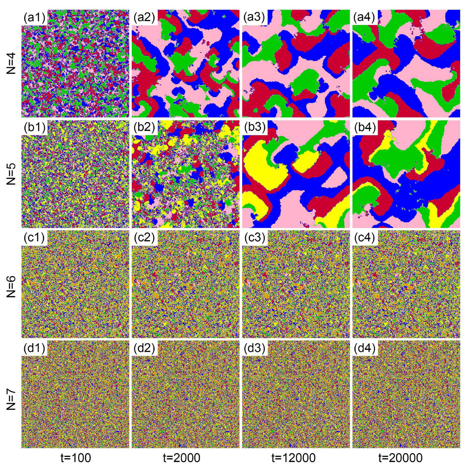
Figure 5.
Temporal variations in population densities of vegetation species for each system illustrated in Figure 4. Panels (a)-(d) correspond to systems with vegetation species, respectively, and curves of different colors represent the population densities of distinct vegetation species.
Figure 5.
Temporal variations in population densities of vegetation species for each system illustrated in Figure 4. Panels (a)-(d) correspond to systems with vegetation species, respectively, and curves of different colors represent the population densities of distinct vegetation species.
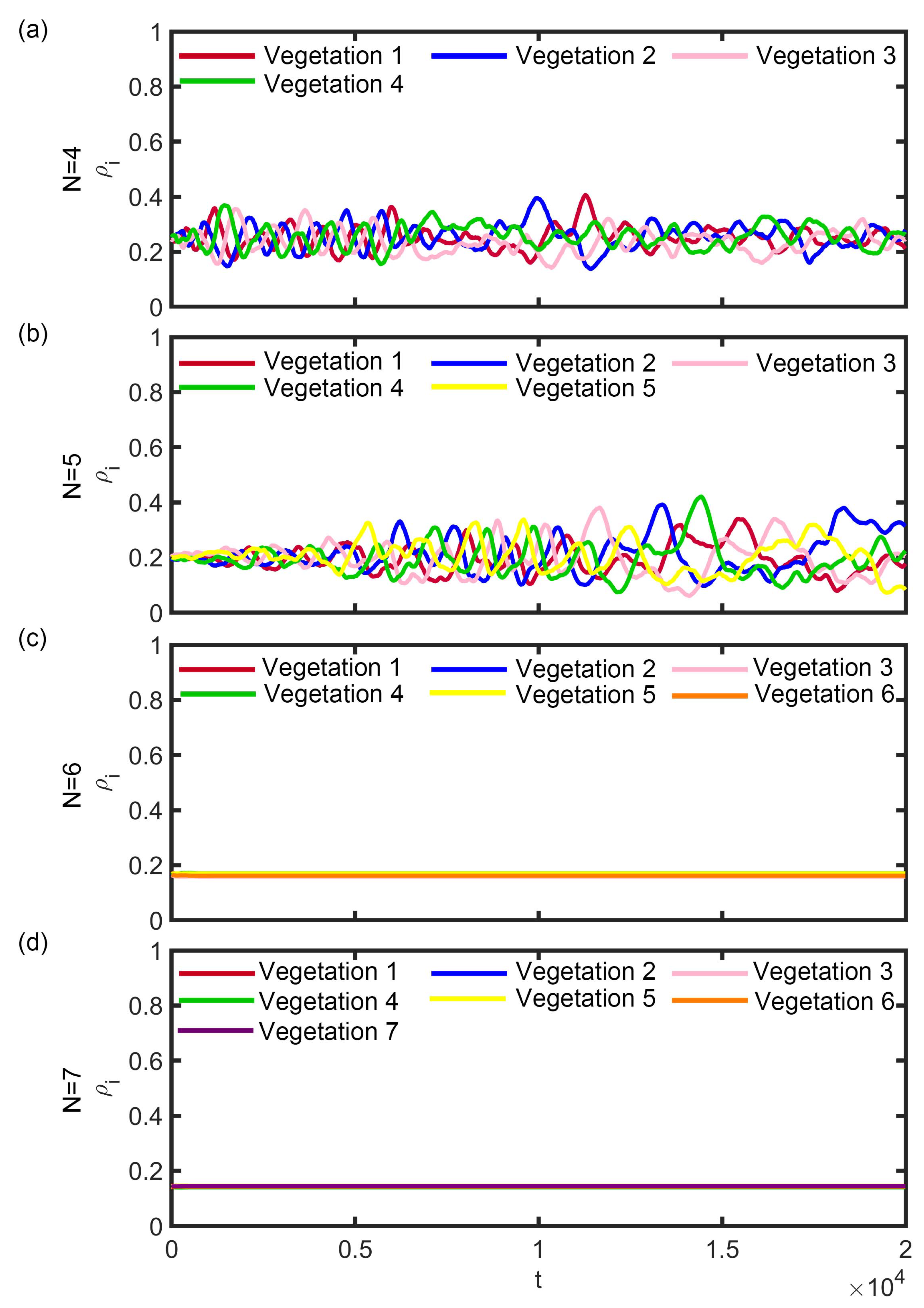
Figure 6.
Evolution of six-species and seven-species vegetation systems at noise intensity . Panels (a & b) depict the spatial pattern evolution, while panels (c & d) illustrate the temporal variations in population densities.
Figure 6.
Evolution of six-species and seven-species vegetation systems at noise intensity . Panels (a & b) depict the spatial pattern evolution, while panels (c & d) illustrate the temporal variations in population densities.
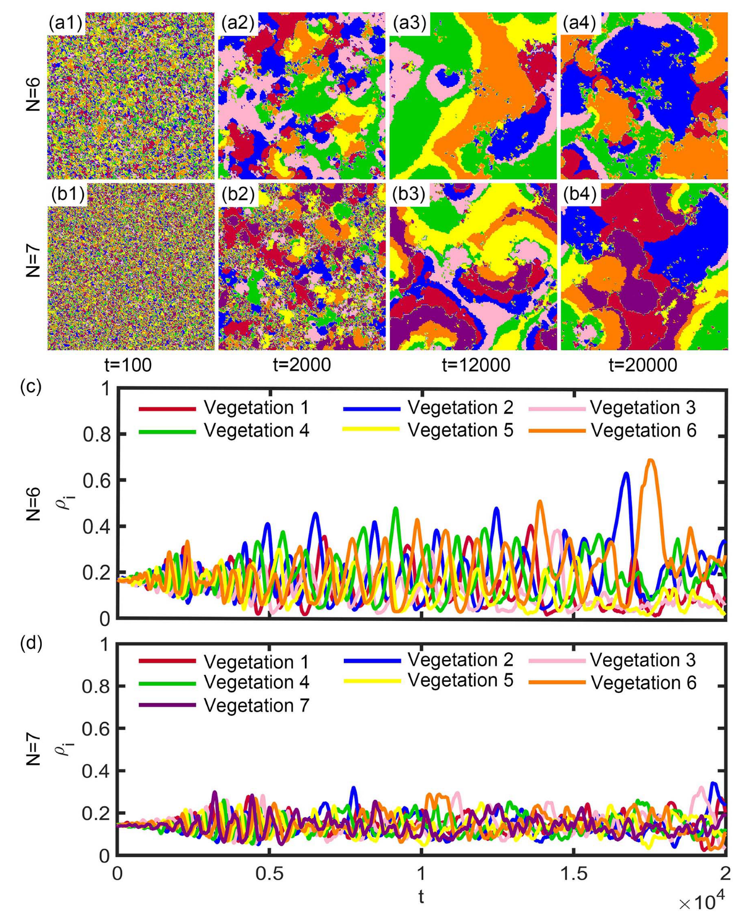
Figure 7.
Distribution of the probability of dynamic equilibrium of the system over the parameter plane. Colors denote the probability that the system remains in an oscillatory state, and the values are averaged from 100 independent replicate simulations.
Figure 7.
Distribution of the probability of dynamic equilibrium of the system over the parameter plane. Colors denote the probability that the system remains in an oscillatory state, and the values are averaged from 100 independent replicate simulations.
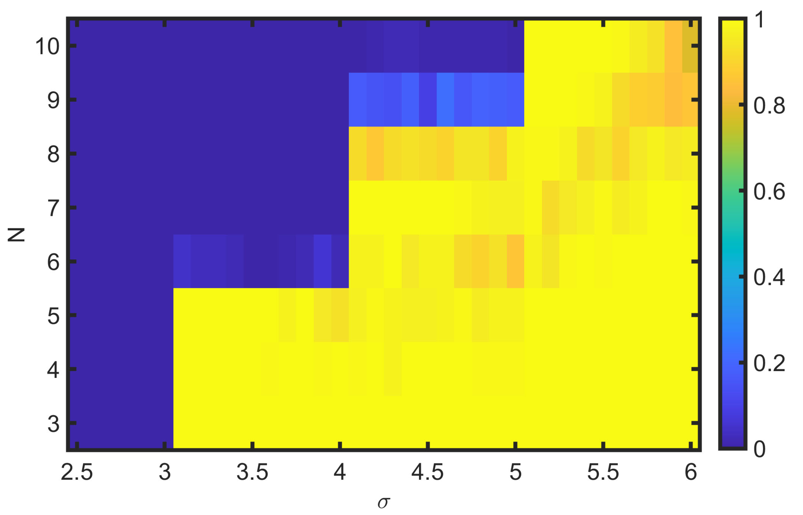
Figure 8.
Temporal evolution of vegetation population densities derived from Eq. (1). Panels (a)-(e) correspond to systems with initial species numbers , respectively.
Figure 8.
Temporal evolution of vegetation population densities derived from Eq. (1). Panels (a)-(e) correspond to systems with initial species numbers , respectively.
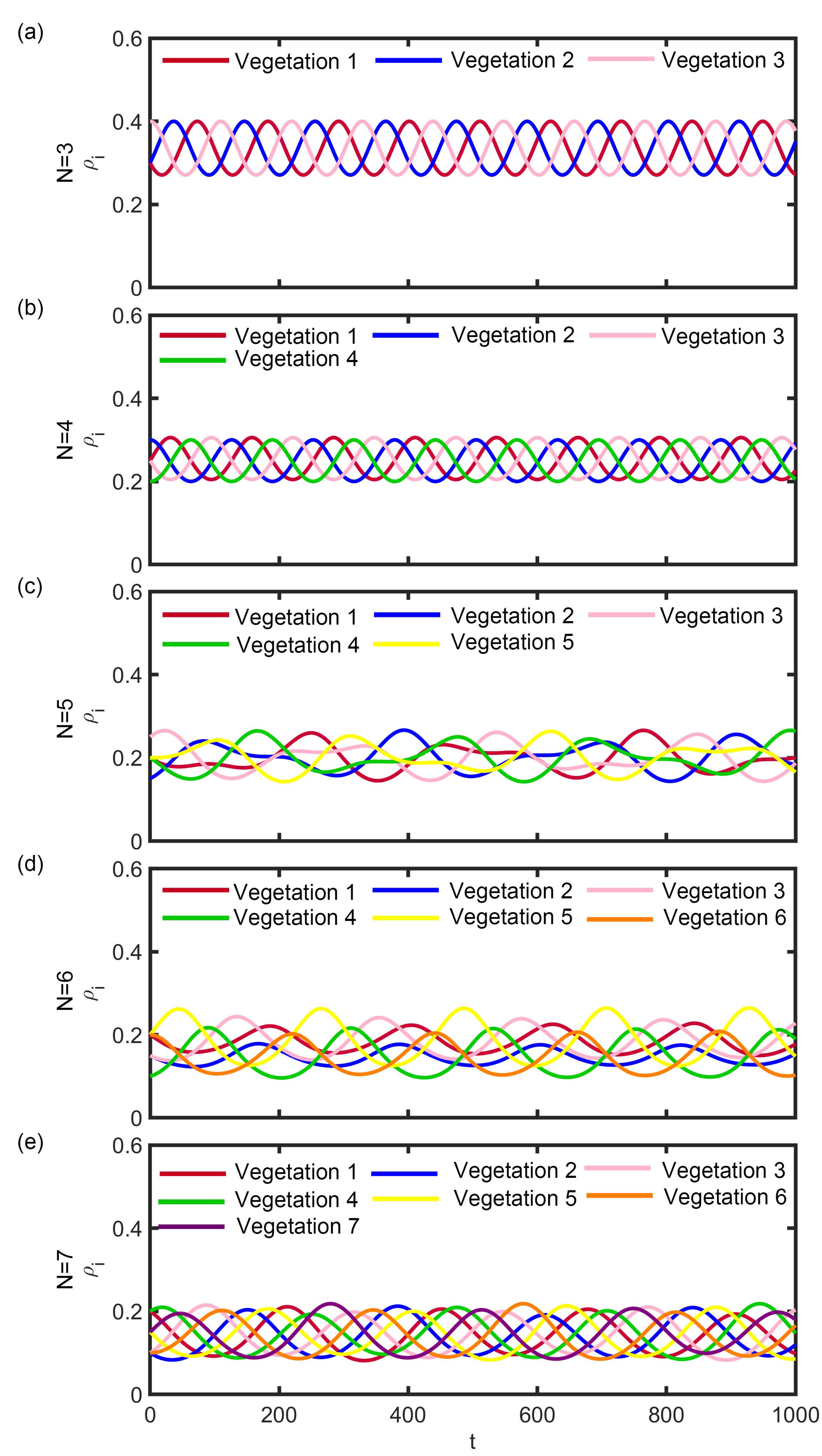
Figure 9.
Spatial patterns of vegetation obtained from Eq. (2). Panels (a)-(f) correspond to systems with initial species quantities , respectively. Different vegetation species are distinguished by distinct colors, and each lattice site is colored according to the vegetation with the maximum population density at that location.
Figure 9.
Spatial patterns of vegetation obtained from Eq. (2). Panels (a)-(f) correspond to systems with initial species quantities , respectively. Different vegetation species are distinguished by distinct colors, and each lattice site is colored according to the vegetation with the maximum population density at that location.
Disclaimer/Publisher’s Note: The statements, opinions and data contained in all publications are solely those of the individual author(s) and contributor(s) and not of MDPI and/or the editor(s). MDPI and/or the editor(s) disclaim responsibility for any injury to people or property resulting from any ideas, methods, instructions or products referred to in the content. |
© 2026 by the authors. Licensee MDPI, Basel, Switzerland. This article is an open access article distributed under the terms and conditions of the Creative Commons Attribution (CC BY) license (http://creativecommons.org/licenses/by/4.0/).
Copyright: This open access article is published under a Creative Commons CC BY 4.0 license, which permit the free download, distribution, and reuse, provided that the author and preprint are cited in any reuse.