

Submitted:
09 July 2026
Posted:
10 July 2026
You are already at the latest version
Abstract
Transportation planning in regions with insufficient public transit often relies on observed travel volumes, overlooking unmanifested latent demand. This study proposes a method to estimate latent travel demand (LTD) within a few kilometers of residential areas using open data—population distribution, aggregated activity data, and facility locations—and investigates its validity and regional variation across three Japanese prefectures (Hiroshima, Ibaraki, and Iwate). Validity was assessed by examining the relationship between estimated LTD and observed travel volumes (apparent traffic volume, ATV) derived from smartphone GPS data. Three key findings emerged. First, LTD, combined with facility count, transit availability, and distance, explained observed travel volumes with R2 = 0.61–0.63 on the original scale and R2 > 0.91 on the log–log scale, and likelihood ratio tests confirmed that LTD provides information complementary to, and distinct from, conventional accessibility indicators. Second, regional fixed-effects analysis revealed that while LTD is a significant predictor across all regions, the demand realization rate (ATV/LTD) varies systematically—from 0.021 in transit-rich Hiroshima to 0.045 in car-dependent Iwate—reflecting differences in transit infrastructure and car dependency. The interaction between LTD and transit availability was statistically significant (p = 0.008), with moderate-transit areas showing the largest marginal effect of LTD on realized travel. Third, activity-type analysis showed that mandatory activities (e.g., medical visits, childcare) maintain stable demand realization regardless of transit levels, while discretionary activities (e.g., hobbies, leisure) are strongly transit-dependent. These results demonstrate that LTD estimation offers a practical, scalable diagnostic tool for identifying mobility gaps and prioritizing transit investments in resource-constrained municipalities.
Keywords:
latent travel demand
; open data
; demand realization rate
; regional variation
; transportation planning
1. Introduction
In regions with insufficient public transportation, such as mountainous and rural areas, securing daily mobility within a few kilometers of home remains a critical challenge [19]. New local transportation modes—including personal mobility devices and low-speed vehicles—have emerged in recent years to address this need. To deploy these modes effectively, it is essential to understand latent travel demand, the potential for travel that is not captured by observed travel volumes, particularly in areas where limited transport options suppress trip-making.
Historically, travel demand has been estimated through person-trip surveys, four-step estimation techniques [1], and activity-based models [11]. Person-trip surveys capture manifest trips but fail to account for latent demand and are seldom conducted in rural areas. Four-step methods are limited by coarse trip-purpose categorization and large spatial zones. Activity-based models comprehensively represent individual behaviors but require disaggregated data and substantial computational resources, making them inaccessible to many small and medium-sized municipalities [13].
This study develops a complementary approach that estimates latent travel demand within a few kilometers of residential areas using aggregated open data—population distribution, activity rates, and facility locations—without requiring individual-level data. The proposed method can be applied to any municipality in Japan where these datasets are available. The study then addresses three research questions:
- 1.
- Validity: Does the estimated LTD bear a significant and meaningful relationship with observed travel volumes, and is this relationship distinct from conventional accessibility measures?
- 2.
- Regional variation: How does the relationship between LTD and realized travel differ across regions with varying transit infrastructure, and what factors explain these differences?
- 3.
- Activity-type heterogeneity: Do mandatory and discretionary activities exhibit different demand realization patterns in response to transit availability?
The analysis covers three Japanese prefectures—Hiroshima, Ibaraki, and Iwate—representing diverse mobility environments from tram-served urban areas to car-dependent rural regions. By examining how latent demand translates into actual travel under varying conditions, this study contributes a diagnostic framework for identifying mobility gaps and informing transit planning in resource-constrained municipalities.
Figure 1 illustrates the conceptual framework of this study. Residents engage in activities, some of which generate a need to move. This need, at the planning and scheduling stages, constitutes latent travel demand. Depending on available transport modes, a portion of this demand is realized as observed travel, while the remainder represents unmet mobility needs.
2. Literature Review
2.1. Approaches to Capturing Travel Demand
Two main approaches exist for capturing travel demand in transportation planning: utilizing observed realized travel volumes and estimating latent (potential) travel demand. The former is effective in urban areas where traffic volumes are substantial and reasonably represent underlying demand [16,18]. Various methods have been developed to measure realized volumes, including smartphone location data [18], taxi trip records [9], and econometric models linking observed travel with transport-level variables [17].
However, in areas with low travel volumes or limited daily travel options, observed volumes may substantially underrepresent actual mobility needs. Clifton and Moura [6] conceptualized latent demand along six stages from unimaginable behaviors to materialized travel. Travel demand fundamentally originates from residents who wish to engage in desired activities [4,12], and activity-based models have been developed to capture this process [2,3,8]. Yet these models require disaggregated individual data and considerable computational resources.
Table 1 compares existing approaches along key dimensions. The proposed method occupies an intermediate position: it incorporates activity-based logic using aggregated data, enabling application in municipalities lacking the resources for full activity-based modeling.
2.2. Latent Travel Demand and Accessibility
Latent travel demand may appear conceptually similar to accessibility indicators used in transportation planning [7,10]. Traditional accessibility measures quantify the supply side of mobility—the ease of reaching opportunities from a given location—using formulations such as:
where represents opportunities at destination j and is a distance-decay function.
In contrast, latent travel demand represents the demand side—quantifying the population’s desire and need to undertake travel-requiring activities at specific times and locations. While accessibility asks “What opportunities can be reached?”, latent demand asks “Who needs to reach what, and when?” This distinction is empirically tested in Section 3.2.2.
2.3. Regional Variation in Travel Behavior
Travel behavior varies substantially across regions with different transportation infrastructure. Car-dependent rural areas exhibit different trip-making patterns than transit-served urban areas. However, most demand estimation methods do not explicitly model how the relationship between potential demand and realized travel varies with regional characteristics.
The concept of a “demand realization rate”—the proportion of latent demand that materializes as observed travel—provides a useful analytical lens. Regions where a smaller fraction of latent demand is realized may represent areas with unmet mobility needs, offering targets for transit investment. This study introduces this concept and analyzes its determinants.
3. Materials and Methods
3.1. Estimation of Latent Travel Demand
3.1.1. Conceptual Framework
Latent travel demand is defined as the number of desired activities requiring travel at the planning and scheduling stages [6]. Following Chapin [4] and Kitamura et al. [12], travel is understood as deriving from people’s desired activities. The estimation integrates three open datasets: population distribution (who, from where), facility distribution (for what purpose, to where), and activity rates (when, who, for what purpose) (Figure 2).
3.1.2. Mathematical Formulation
Table 2 defines the key variables used throughout this paper.
Latent travel demand is calculated as:
3.1.3. Estimation Procedure
The estimation followed four steps (Figure 3):
Step 1: Calculate the activity-specific population by time of day for each 500 m mesh:
Step 2: Apply the trip generation rate to estimate latent demand:
Step 3: Allocate demand to nearest facilities within 1, 3, and 5 km radii using a distance-decay function.
Step 4: Aggregate all activity-specific demands to construct the origin–destination matrix:
Table 3 summarizes the correspondence between activities, facilities, and trip generation rates.
3.1.4. Data Sources
Population distribution data were sourced from the National Land Numerical Information database (MLIT) at mesh resolution, disaggregated by age and sex. Facility distribution data were collected from open online maps, covering 20 facility types associated with travel activities. Activity data were obtained from the NHK Time Use Survey, providing aggregated proportions of the population engaged in specific activities by age, sex, and time of day.
3.2. Validation Framework
3.2.1. Realized Travel Model
Since latent travel demand is inherently unobservable, validation was conducted indirectly. The core logic is that if LTD estimates are valid, they should strongly explain observed travel volumes when combined with supply-side factors representing the realization process:
Figure 4 illustrates this conceptual model. Latent travel demand, estimated from open data (population, activity, and facility distributions), transforms into realized travel through supply-side factors—facility count, transit availability (number of buses/railways and stations), and distance—within 1, 3, and 5 km radii from residential areas. Realized travel is observed through Probe Person Data (smartphone GPS).
The explanatory power () and statistical significance of the LTD variable serve as evidence for the validity of the estimation approach. Six model specifications (Models 1–6) were estimated, varying in functional form, estimation method, and distributional assumptions (see Section 4.3.1 for details).
Observed traffic volumes were derived from Konzatsu-Tokei® data, based on anonymized smartphone GPS records from consenting NTT DOCOMO users. These data provide daily visitor counts to each 500 m mesh (excluding residents), stratified by distance from home. Half-day records were aggregated to daily totals.
3.2.2. Comparison with Accessibility Measures
To empirically test whether LTD provides information distinct from accessibility, a Hansen-type accessibility index was computed:
where is the number of facilities and is the distance band midpoint (0.5, 2.0, 4.0, or km). Four competing models were estimated:
- Model A: (demand-side only)
- Model B: (supply-side only)
- Model C: (combined)
- Model D: (full model)
Likelihood ratio tests (LRT) assessed whether each variable adds significant information beyond the other.
3.2.3. Robustness Checks
Sensitivity to trip generation rate: Since values were derived from national statistics and may not reflect local conditions, the trip generation rate was varied by ±10%, ±20%, and ±30%, and models were re-estimated to assess result stability.
Spatial autocorrelation: Moran’s I statistic was computed on model residuals to test for spatial autocorrelation, using a K-nearest-neighbor spatial weights matrix () constructed from mesh centroid coordinates.
3.3. Regional Variation Analysis
3.3.1. Regional Fixed-Effects Model
To examine whether the LTD–ATV relationship varies across regions, prefecture dummy variables were introduced:
An interaction model further tested whether the LTD effect itself differs by region:
A likelihood ratio test (analogous to Chow test) assessed the significance of regional differences.
3.3.2. Demand Realization Rate
The demand realization rate was defined as:
An OLS regression examined the determinants of log-transformed realization rate:
3.3.3. Transit as Moderator
The moderating effect of transit availability on the LTD–ATV relationship was tested through an interaction term (). Additionally, the sample was stratified into three transit-level groups (Low, Medium, High) based on tertiles, and separate models were estimated for each group.
3.4. Study Areas and Data
Three Japanese prefectures were selected to represent diverse mobility environments:
- Hiroshima: Tram-served urban area with 48% car use and 6.2% public transport share.
- Ibaraki: Suburban area served by JR Joban Line and Tsukuba Express, with 68% car use and 5.3% public transport share.
- Iwate: Car-dependent rural area with limited rail access (JR Tohoku Main Line), 70% car use and 3.4% public transport share.
Geospatial processing was performed in QGIS, with statistical estimation in Python using statsmodels and scipy. Data from the three prefectures were pooled for the primary analysis, with regional heterogeneity explicitly modeled through fixed effects and interaction terms.
4. Results
4.1. Descriptive Statistics
Table 4 presents the descriptive statistics. The three prefectures exhibit distinct mobility profiles. Hiroshima, with the highest transit operations (mean = 1,077), shows moderate ATV (40.1) despite high LTD (1,867). Iwate, with the lowest transit availability (370), shows the highest ATV (50.1) relative to its moderate LTD (1,115). These patterns foreshadow the regional variation in demand realization analyzed in Section 4.4.
4.2. Estimation of Latent Travel Demand
Figure 6 presents the temporal and spatial patterns of estimated latent travel demand. Commuting and school travel were excluded, as individuals with personal vehicles have lower priority for mobility support, and school travel demands can be identified through separate surveys.
Morning demand (6:00–8:00) concentrates on leisure and sports facilities; midday demand (10:00–15:00) shifts toward shopping and medical facilities; and evening demand (17:00–19:00) peaks for childcare-related travel. The OD lines demonstrate spatially concentrated corridors linking residential meshes to facility clusters.
4.3. Validation of the LTD Estimation Method
4.3.1. Realized Travel Models
Table 6 summarizes the estimation results across six model specifications, and Figure 7 presents the observed vs. predicted scatter plots. Models 1–2 (OLS with log-transformed ATV) yielded values of 0.61–0.62. Model 3 (Poisson GLM) showed similar performance. Models 4–6, which applied logarithmic transformations to both dependent and explanatory variables, substantially improved model performance, explaining over 90% of the variance (–). In all models, the LTD coefficient was highly significant (), confirming that estimated latent demand is a strong predictor of observed travel volumes.
The substantial difference in between Models 1–3 (0.61–0.63) and Models 4–6 (0.91–0.92) warrants discussion. The log–log specification (Models 4–6) compresses variance in both dependent and explanatory variables, which mechanically inflates relative to models on the original scale. Models 1–3, which do not apply logarithmic transformation to the explanatory variables, provide a more conservative estimate of explanatory power. Ten-fold cross-validation on the original (non-log) scale yielded an out-of-sample of 0.61 (Section 4.3.3), further confirming that the model’s predictive performance on the original scale is moderate rather than exceptionally high. Importantly, the LTD coefficient remains highly significant () across all six specifications regardless of functional form, indicating that the finding of LTD as a meaningful predictor of observed travel volumes is not an artifact of the logarithmic transformation.
4.3.2. Distinction from Accessibility Measures
Table 7 presents the comparison between LTD and accessibility-based models. LTD alone (Model A) explains 55.1% of ATV variance, while accessibility alone (Model B) performs poorly (). When both are included (Model C), both LTD (, ) and accessibility (, ) are significant, indicating complementary information.
Likelihood ratio tests confirmed that each variable adds significant information beyond the other (Table 8).
The asymmetry in values (467,726 vs. 6,826) indicates that LTD contributes far more explanatory power than accessibility, consistent with the view that demand-side information is more fundamental than supply-side information for explaining realized travel.
4.3.3. Robustness Checks
Sensitivity to trip generation rate: Table 9 shows that varying p by ±30% produces negligible changes in model performance ( range: 0.626–0.627; RMSE change < 0.1%). The LTD coefficient adjusts slightly but remains highly significant across all specifications.
Spatial autocorrelation: Moran’s I test on mesh-level model residuals yielded (, ), indicating no significant spatial autocorrelation (Supplementary Figure S1). This confirms that the non-spatial GLM estimation is appropriate and residuals are spatially independent.
Cross-validation: Ten-fold random cross-validation on the pooled data yielded an average out-of-sample of 0.61 on the original scale and 0.79 on the log scale, with an average correlation of , confirming model stability and absence of overfitting.
4.4. Regional Variation in Demand Realization
4.4.1. Regional Fixed-Effects Models
Table 10 presents the estimation results for pooled, fixed-effects, and interaction models. The likelihood ratio test strongly rejects the pooling assumption (, , ), confirming significant regional differences.
Three important findings emerge. First, the core variables (LTD, facilities, transit, distance) maintain consistent signs and significance across all specifications, confirming the structural validity of the model. Second, Ibaraki shows a significantly lower intercept (), reflecting its lower baseline ATV, while Iwate shows a higher intercept (). Third, and most notably, the interaction term for Iwate (, ) indicates that the effect of LTD on realized travel is substantially stronger in this car-dependent rural prefecture. The interaction for Ibaraki is not significant (), suggesting a similar LTD effect structure to Hiroshima.
4.4.2. Determinants of Demand Realization
Table 11 presents the OLS regression of log-transformed realization rate on supply-side factors.
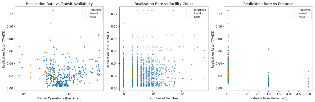
The realization rate is positively associated with facility count (): more facilities enable more demand to be realized. Distance has a strong negative effect (): demand farther from home is less likely to be realized. The transit coefficient is negative (), which may appear counterintuitive but reflects that transit-rich areas (urban centers) have higher population densities, generating larger LTD denominators while ATV does not increase proportionally.
After controlling for these factors, the Iwate dummy remains significantly positive (), indicating that car-dependent regions exhibit higher demand realization. This is consistent with the interpretation that in areas without public transit alternatives, residents rely on private vehicles, resulting in more latent demand being manifested as actual travel.
Figure 8.
Demand realization rate (ATV/LTD) vs. (a) transit availability, (b) facility count, and (c) distance from home. Colors indicate prefectures: blue = Hiroshima, orange = Ibaraki, green = Iwate.
Figure 8.
Demand realization rate (ATV/LTD) vs. (a) transit availability, (b) facility count, and (c) distance from home. Colors indicate prefectures: blue = Hiroshima, orange = Ibaraki, green = Iwate.
4.4.3. Transit as Moderator of Demand Realization
Table 12 shows that the interaction between and is statistically significant (, ), indicating that transit availability moderates the LTD–ATV relationship.
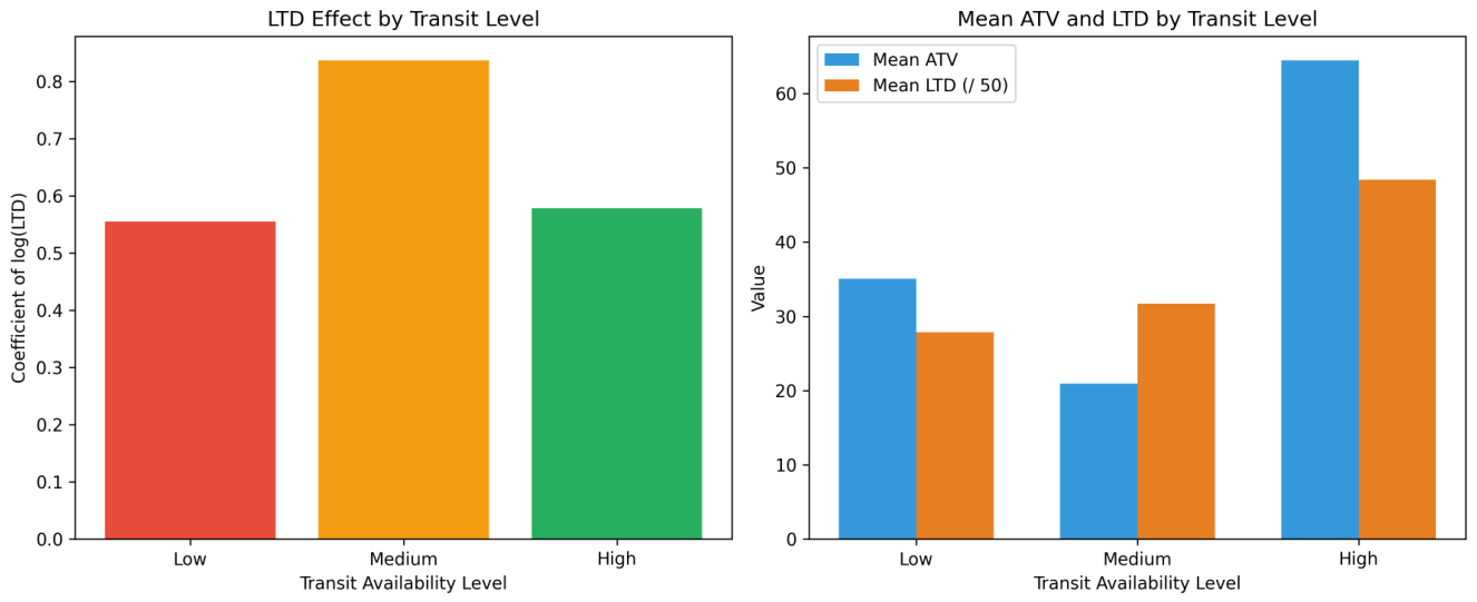
Subgroup analysis by transit level (Table 13) reveals a non-linear pattern: the LTD coefficient is highest in the medium-transit group (), compared to low-transit () and high-transit () groups. This suggests that the marginal effect of latent demand on realized travel is greatest at moderate transit service levels—a “sweet spot” where transit improvements yield the largest gains in demand realization.
Figure 9.
LTD effect by transit availability level. (a) Coefficient of by transit level. (b) Mean ATV and LTD by transit level.
Figure 9.
LTD effect by transit availability level. (a) Coefficient of by transit level. (b) Mean ATV and LTD by transit level.
4.5. Activity-Type Analysis by Transit Level
Table 14 presents the LTD coefficients by activity type, stratified by transit availability.
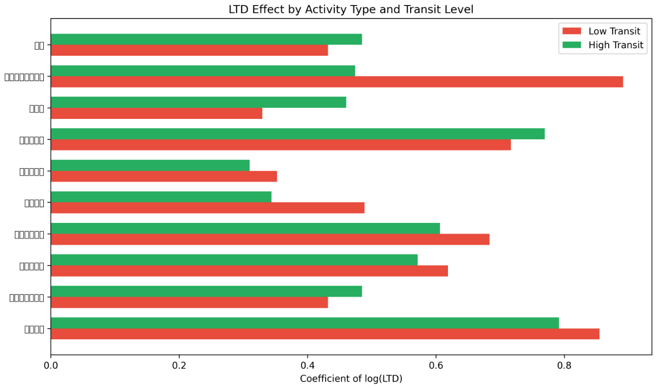
For mandatory activities such as medical care ( vs. 0.310) and childcare ( vs. 0.606), the LTD coefficient is relatively stable across transit levels. These are essential activities that residents undertake regardless of transit availability, likely using private vehicles when public transit is unavailable.
In contrast, hobbies and entertainment show a striking difference: in low-transit areas vs. 0.474 in high-transit areas. The high coefficient in low-transit areas suggests that there is substantial latent demand for cultural and recreational activities that goes unrealized due to transportation constraints. This represents a clear mobility gap that transit improvements could address.
Shopping shows the opposite pattern ( in low-transit vs. 0.460 in high-transit areas), suggesting that transit availability enables shopping trips that would otherwise not occur.
Figure 10.
LTD coefficient () by activity type, stratified by transit level. Red = low transit; green = high transit.
Figure 10.
LTD coefficient () by activity type, stratified by transit level. Red = low transit; green = high transit.
5. Discussion
5.1. Validity of the LTD Estimation Approach
The results provide strong evidence for the validity of the proposed LTD estimation method. First, LTD is a highly significant predictor of observed travel volumes across all model specifications (Table 6). On the original (non-log) scale, Models 1–3 explain 61–63% of ATV variance; on the log–log scale, Models 4–6 explain 91–92%. The higher in the log–log specifications reflects variance compression inherent in the logarithmic transformation rather than a fundamentally different level of predictive accuracy. Ten-fold cross-validation on the original scale yielded an out-of-sample of 0.61, providing a conservative but reliable estimate of predictive performance. Critically, the LTD coefficient is highly significant () in all six specifications, confirming that the finding is robust to functional form choice. Second, LTD provides information that is statistically distinct from conventional accessibility measures (Table 7 and Table 8): likelihood ratio tests confirm that LTD adds substantial explanatory power beyond accessibility (), while accessibility adds comparatively modest information beyond LTD (). This asymmetry supports the theoretical distinction that LTD captures demand-side information (“who needs to travel”) while accessibility captures supply-side information (“what can be reached”). Third, the results are robust to parameter sensitivity (±30% variation in p produces <0.1% change in RMSE) and free from spatial autocorrelation (Moran’s , ).
These findings address the fundamental validation challenge: since latent demand is unobservable, it cannot be validated directly. Our approach demonstrates validity indirectly but convincingly, by showing that LTD estimates, when combined with supply-side factors representing the realization process, produce strong, robust, and theoretically consistent explanations of observed travel patterns.
5.2. Regional Variation and Its Interpretation
The regional variation in the LTD–ATV relationship is perhaps the most substantively interesting finding. The demand realization rate varies from 0.021 in Hiroshima to 0.045 in Iwate (Table 5), and the fixed-effects analysis confirms that this variation is statistically significant (Chow test, ). Moreover, the interaction analysis reveals that the LTD effect is substantially stronger in Iwate (, ).
These patterns are interpretable through the lens of regional transport infrastructure:
Hiroshima (low realization rate, high transit): With extensive tram and bus networks, Hiroshima has a large population generating substantial latent demand. However, the high LTD denominator—driven by population density—means that the ratio of realized to latent demand is relatively low. This does not indicate poor mobility; rather, it reflects that dense urban populations generate latent demand across many activities, only a fraction of which translates to observable travel to any given mesh.
Iwate (high realization rate, low transit): In this car-dependent rural region, limited public transit options mean residents must rely on private vehicles. Consequently, a larger fraction of latent demand is manifested as observed travel—residents travel because they have no alternative. The higher LTD coefficient ( for Iwate vs. 0.599 for Hiroshima; Table 13) is consistent with this interpretation: each unit of latent demand translates more directly into actual travel in car-dependent areas.
Ibaraki (intermediate): With moderate transit infrastructure, Ibaraki falls between the extremes, showing intermediate realization rates and LTD coefficients.
5.3. Policy Implications
The demand realization framework offers several practical applications for transportation planners:
Identifying mobility gaps: The gap between estimated LTD and observed ATV quantifies unmet mobility needs at the mesh level. Meshes with high LTD but low realization rates represent priority areas for transit investment.
Prioritizing transit improvements: The subgroup analysis (Table 13) reveals that moderate-transit areas show the largest LTD coefficient (), suggesting that transit improvements yield the greatest marginal effect on demand realization at intermediate service levels. This finding can guide resource allocation toward areas where investment would have the highest impact.
Activity-specific planning: The activity-type analysis (Table 14) identifies which types of demand are most suppressed by limited transit. Hobbies and entertainment show the largest gap between low- and high-transit areas (), indicating substantial unmet demand for cultural and recreational mobility. Conversely, shopping shows higher realization in transit-rich areas, suggesting that transit improvements can unlock new shopping trips.
Benchmarking across regions: The realization rate enables comparisons across municipalities. Regions with the lowest realization rates, controlling for structural factors, can be identified as underserved. Data Envelopment Analysis (DEA) could be applied to benchmark regional performance [5].
5.4. Limitations and Future Work
Several limitations should be noted. First, the analysis focuses on single-purpose trips, excluding trip chains that commonly occur in daily travel behavior. Second, the study covers three prefectures; while these represent diverse mobility environments, validation across additional regions would strengthen generalizability. Third, trip generation rates (p) were derived from national-level statistics and may not perfectly reflect local conditions, although sensitivity analysis shows the results are robust to ±30% variation. Fourth, distance thresholds (1, 3, and 5 km) were selected to represent typical short-distance daily travel but lack empirical justification specific to the study areas. Fifth, the model excludes commuting, school, and tourism trips. Sixth, it does not account for facility attractiveness or quality, treating all facilities of the same type equally. Seventh, sample sizes for Ibaraki () and Iwate () are substantially smaller than for Hiroshima (), which may limit the statistical power of prefecture-specific analyses.
Future research should address five areas. First, incorporating trip chains would more accurately represent daily travel patterns. Second, expanding to additional prefectures and using multilevel modeling would enable more robust treatment of regional heterogeneity. Third, developing local calibration methods for trip generation rates using limited local survey data could improve accuracy. Fourth, integrating the demand realization framework with DEA would provide a formal benchmarking tool for regional transportation planning. Fifth, applying the method to evaluate specific policy scenarios (e.g., new transit routes, facility relocations) would demonstrate its practical utility.
6. Conclusions
This study developed a method to estimate latent travel demand using open data and investigated its validity and regional variation through analysis of three Japanese prefectures. Three principal findings emerged:
First, the proposed LTD estimation method produces valid demand estimates. LTD, combined with supply-side factors, explains 61–63% of observed travel volume variance on the original scale and over 90% on the log–log scale; the higher in the latter reflects variance compression due to the logarithmic transformation. LTD provides information that is empirically distinct from accessibility indicators, contributing substantially more explanatory power in likelihood ratio tests. The estimation is robust to parameter choices and free from spatial autocorrelation.
Second, the relationship between latent demand and realized travel varies systematically across regions. Car-dependent rural areas (Iwate) show higher demand realization rates and stronger LTD effects, while transit-rich urban areas (Hiroshima) show lower realization rates. The interaction between LTD and transit availability is statistically significant, with the marginal effect of LTD on realized travel being greatest at moderate transit service levels.
Third, mandatory activities (medical care, childcare) exhibit stable demand realization regardless of transit availability, while discretionary activities (hobbies, entertainment) show large differences between transit-rich and transit-poor areas, indicating substantial unmet demand in underserved regions.
These findings contribute to both methodology and practice. Methodologically, the study demonstrates that latent travel demand can be estimated from publicly available aggregated data without individual-level surveys, and introduces the demand realization rate as a diagnostic indicator for regional mobility assessment. Practically, the approach provides resource-constrained municipalities with a scalable tool for identifying where, when, and for what purposes mobility needs remain unmet, enabling evidence-based prioritization of transit investments.
Author Contributions
Takashi Kobayashi: Conceptualization, Methodology, Software, Validation, Formal analysis, Investigation, Data curation, Writing—original draft, Writing—review & editing, Visualization.
Data Availability Statement
The population distribution data are publicly available from the National Land Numerical Information download service (https://nlftp.mlit.go.jp/). Activity rate data are available from the NHK Broadcasting Culture Research Institute Time Use Survey. The observed travel volume data (Konzatsu-Tokei, a registered trademark of NTT DOCOMO) were obtained under a data use agreement and are not publicly available due to licensing restrictions. Processed analysis results are available from the author upon reasonable request.
Acknowledgments
This research received no external funding. Generative AI tools (Anthropic Claude) were used to assist with English-language editing and manuscript preparation; the author reviewed all output and takes full responsibility for the content.
Conflicts of Interest
The author declares that there are no known competing financial interests or personal relationships that could have appeared to influence the work reported in this paper.
References
- Agrawal, A., Udmale, S.S., Sambhe, V.K., 2018. Extended four-step travel demand forecasting model for urban planning. In: Mishra, D.K., Nayak, M.K., Joshi, A. (Eds.), Information and Communication Technology for Sustainable Development. Springer, Singapore, pp. 469–474.
- Arentze, T.A., Timmermans, H.J.P., 2004. A learning-based transportation oriented simulation system. Transp. Res. B: Methodol. 38 (7), 613–633.
- Bowman, J.L., Ben-Akiva, M.E., 2001. Activity-based disaggregate travel demand model system with activity schedules. Transp. Res. A Policy Pract. 35 (1), 1–28.
- Chapin, F.S., 1974. Human Activity Patterns in the City: Things People Do in Time and in Space. University of Massachusetts at Boston.
- Charnes, A., Cooper, W.W., Rhodes, E., 1978. Measuring the efficiency of decision making units. Eur. J. Oper. Res. 2 (6), 429–444.
- Clifton, K.J., Moura, F., 2017. Conceptual framework for understanding latent demand: accounting for unrealized activities and travel. Transp. Res. Rec. 2668 (1), 78–83.
- Geurs, K.T., van Wee, B., 2004. Accessibility evaluation of land-use and transport strategies: review and research directions. J. Transp. Geogr. 12 (2), 127–140.
- Hägerstrand, T., 1970. What about people in Regional Science? Region. Sci. Assoc. 24 (1), 6–21.
- Hamedmoghadam, H., Ramezani, M., Saberi, M., 2019. Revealing latent characteristics of mobility networks with coarse-graining. Sci. Rep. 9 (1), 7545.
- Hansen, W.G., 1959. How accessibility shapes land use. J. Am. Inst. Plann. 25 (2), 73–76.
- Jones, P.M., 1979. New approaches to understanding travel behaviour: the human activity approach. In: Hensher, D.A., Stopher, P.R. (Eds.), Behavioural Travel Modelling. Routledge, London.
- Kitamura, R., Fujii, S., Pas, E.I., 1997. Time-use data, analysis and modeling: toward the next generation of transportation planning methodologies. Transp. Policy 4 (4), 225–235.
- Liu, Y., Liao, X., Ma, H., He, B.Y., Stanford, C., Ma, J., 2025. Human mobility modeling with household coordination activities under limited information via retrieval-augmented LLMs. In: Proceedings of the IEEE 28th International Conference on Intelligent Transportation Systems (ITSC 2025). IEEE.
- Ministry of Health, Labour and Welfare (MHLW), 2020. Patient Survey (Kanja Chosa). Available at: https://www.mhlw.go.jp/toukei/saikin/hw/kanja/20/.
- Ministry of Internal Affairs and Communications (MIC), 2021. Family Income and Expenditure Survey (Kakei Chosa). Statistics Bureau of Japan. Available at: https://www.stat.go.jp/data/kakei/.
- Noland, R.B., Lem, L.L., 2002. A review of the evidence for induced travel and changes in transportation and environmental policy in the US and the UK. Transp. Res. D: Transp. Environ. 7 (1), 1–26.
- Plakandaras, V., Papadimitriou, T., Gogas, P., 2019. Forecasting transportation demand for the U.S. market. Transp. Res. A: Policy Pract. 126, 195–214.
- Toole, J.L., Colak, S., Sturt, B., Alexander, L.P., Evsukoff, A., Gonzalez, M.C., 2015. The path most traveled: travel demand estimation using big data resources. Transp. Res. C: Emerg. Technol. 58, 162–177.
- Uspalyte-Vitkuniene, R., Bureika, G., Burinskiene, M., Vabuolyte, V., Skrickij, V., 2022. Sharing mobility solutions in remote touristic area: case study of Lithuania. Transport 37 (4), 241–250.
Figure 1.
Definition of latent travel demand. The framework illustrates the stages from unimaginable behaviors to realized travel, following Clifton and Moura [6]. This study focuses on the planning and scheduling stages.
Figure 1.
Definition of latent travel demand. The framework illustrates the stages from unimaginable behaviors to realized travel, following Clifton and Moura [6]. This study focuses on the planning and scheduling stages.
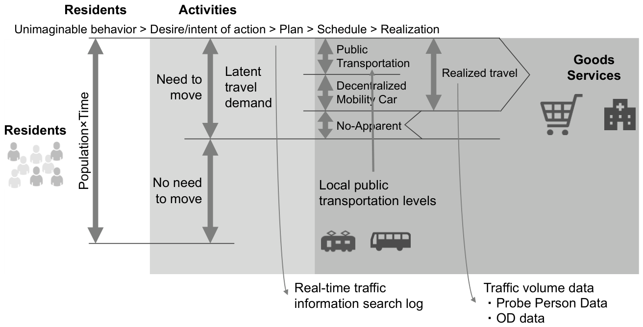
Figure 2.
Three types of open data required for estimating latent travel demand: population distribution (who, from where), facility distribution (for what purpose, to where), and activity rates (when, who, for what purpose).
Figure 2.
Three types of open data required for estimating latent travel demand: population distribution (who, from where), facility distribution (for what purpose, to where), and activity rates (when, who, for what purpose).
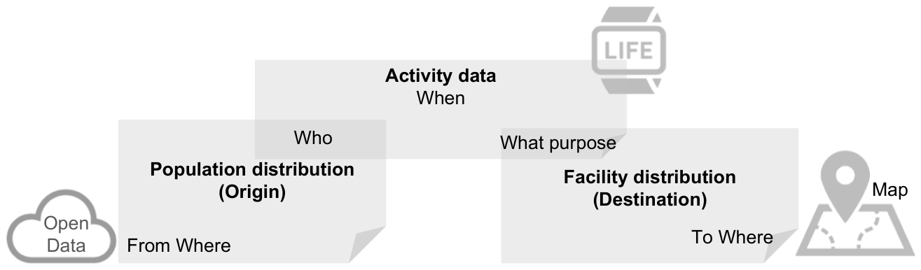
Figure 3.
Procedure for estimating latent travel demand. The four-step process: (1) calculate activity-specific population by time of day (Equation (3)), (2) apply trip generation rates (Equation (4)), (3) allocate demand to nearest facilities, (4) generate OD matrix (Equation (5)).
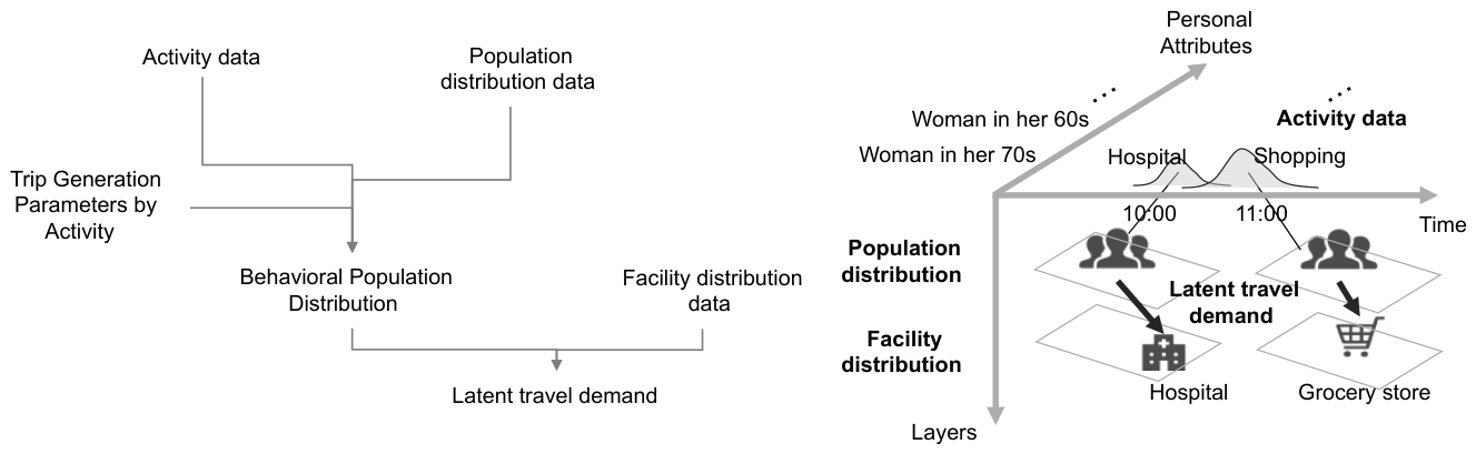
Figure 4.
Conceptual model of demand realization. Latent demand (right) transforms into observed travel (left) through supply-side factors (facilities, transit) and impedance (distance) within concentric distance bands.
Figure 4.
Conceptual model of demand realization. Latent demand (right) transforms into observed travel (left) through supply-side factors (facilities, transit) and impedance (distance) within concentric distance bands.
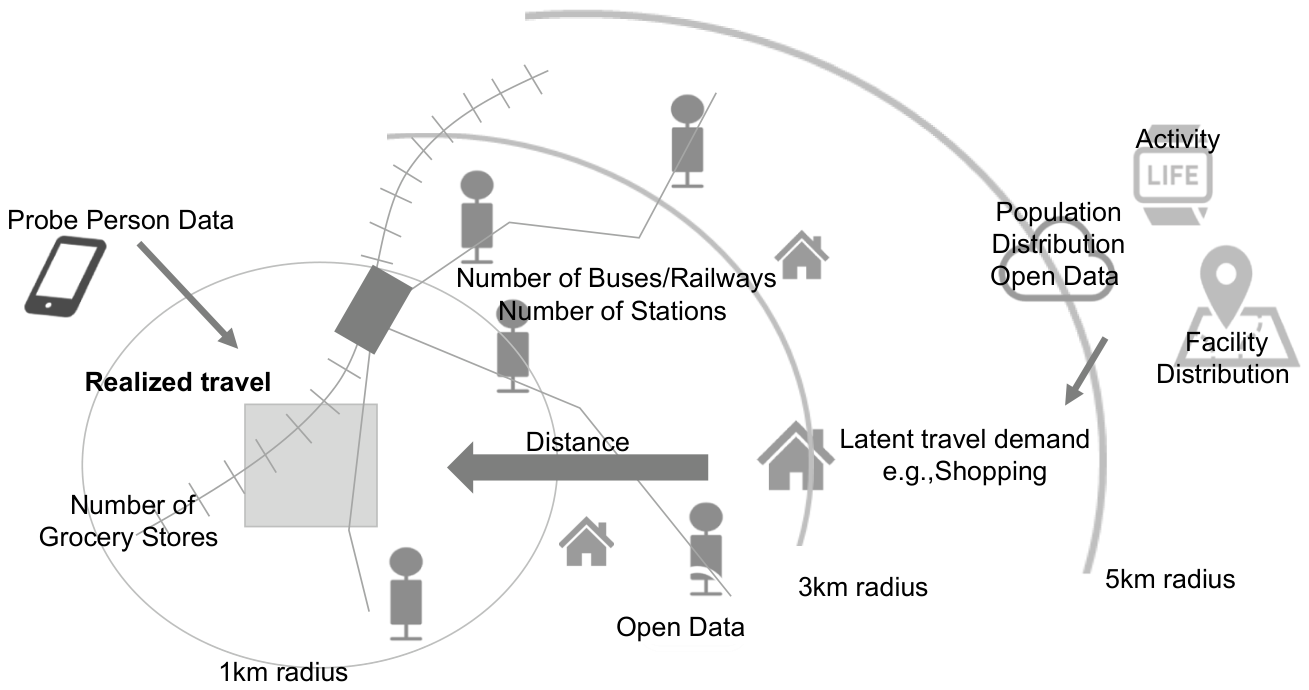
Figure 5.
Core LTD–ATV relationship. (a) LTD vs. ATV by prefecture on original scale. (b) Log–log scale showing linear relationship. (c) Demand realization rate vs. transit availability.
Figure 5.
Core LTD–ATV relationship. (a) LTD vs. ATV by prefecture on original scale. (b) Log–log scale showing linear relationship. (c) Demand realization rate vs. transit availability.
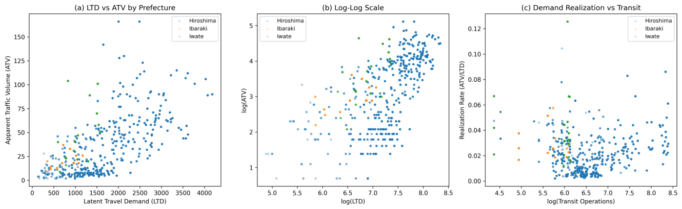
Figure 6.
Temporal and spatial patterns of estimated latent travel demand. Upper: activity rates by time of day. Lower: origin–destination pairs with line thickness proportional to demand volume.
Figure 6.
Temporal and spatial patterns of estimated latent travel demand. Upper: activity rates by time of day. Lower: origin–destination pairs with line thickness proportional to demand volume.
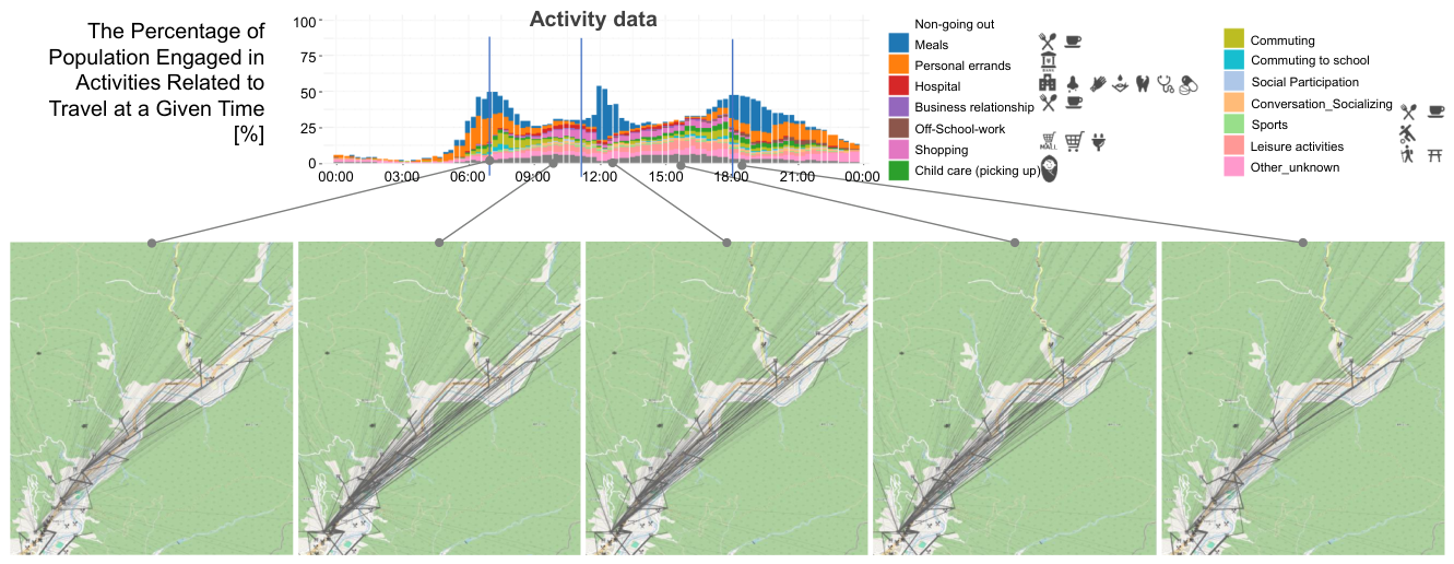
Figure 7.
Observed vs. predicted travel volumes for Models 1–6. Colors indicate distance bands: red = 0–1 km, green = 1–3 km, blue = 3–5 km. The dashed line represents perfect prediction.
Figure 7.
Observed vs. predicted travel volumes for Models 1–6. Colors indicate distance bands: red = 0–1 km, green = 1–3 km, blue = 3–5 km. The dashed line represents perfect prediction.
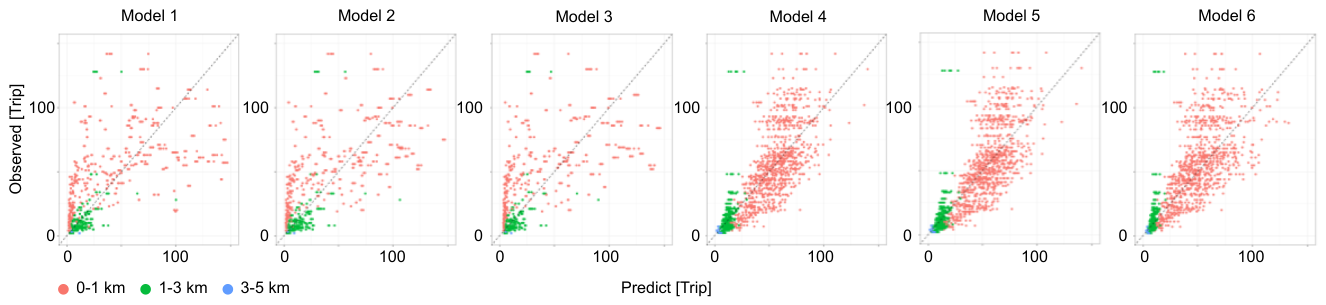

Table 1.
Comparison of travel demand estimation approaches.
| Characteristic | Person-trip | Four-step | Activity-based | Proposed |
| surveys | method | models | method | |
| Captures latent demand | No | Partially | Yes | Yes |
| Fine spatial resolution | No | No | Yes | Yes |
| Time-of-day resolution | Limited | Limited | Yes | Yes |
| Purpose-specific | Limited | Limited | Yes | Yes |
| Individual data required | Yes | Yes | Yes | No |
| Applicable to rural areas | Rarely | Partially | Rarely | Yes |
| Computational resources | Low | Moderate | High | Low |
Table 2.
Variable definitions.
| Variable | Definition | Unit | Data source |
|---|---|---|---|
| Latent travel demand from mesh i for activity j at time k | Persons/day/mesh | Estimated | |
| Apparent traffic volume (observed visitors excl. residents) | Persons/day/mesh | Konzatsu-Tokei® | |
| Population in mesh i (by age and sex) | Persons | Nat’l Land Num. Info. | |
| Activity rate for activity j at time k | Proportion | NHK Time Use Survey | |
| Trip generation rate for activity j (p in Table 3) | Proportion | National statistics | |
| Demand realization rate () | Ratio | Computed |
Table 3.
Correspondence between activities, facilities, and trip generation rates.
| Activity | Facility | Trip generation rate (p) |
|---|---|---|
| Meals | Restaurants | 0.13 |
| Medical care | Hospitals, clinics, pharmacies | 0.039–0.318 |
| Shopping | Supermarkets, malls, electronics | 0.014–0.286 |
| Work-related socializing | Restaurants | 0.90 |
| Childcare | Nursery schools, kindergartens | 0.71 |
| Household chores | Banks, government offices | 0.033 |
| Conversation/Socializing | Cafes | 0.345 |
| Sports | Parks, gyms, fitness centers | 0.14–0.86 |
| Outings/Strolling | Museums, scenic spots, farms | 0.14–0.44 |
| Hobbies/Entertainment | Sports facilities | 0.10 |
Note: p represents the proportion of each activity that generates travel to the corresponding facility type. Medical care rates were calculated from the MHLW Patient Survey [14]; meal-related rates from the Family Income and Expenditure Survey [15]. The sensitivity of results to ±30% variation in these rates is reported in Section 3.2.3.
Table 4.
Descriptive statistics by prefecture (weekday data).
| Variable | Hiroshima | Ibaraki | Iwate | Total |
|---|---|---|---|---|
| N (observations) | 4,281 | 144 | 244 | 4,669 |
| N (meshes) | 242 | 13 | 18 | 273 |
| ATV (mean ± SD) | ||||
| LTD (mean ± SD) | ||||
| Facilities (mean ± SD) | ||||
| Transit ops. (mean ± SD) | ||||
| Distance (mean ± SD) |
Table 5.
Demand realization rate by prefecture.
| Prefecture | Mean RR | Median RR | SD | Mean transit | Mean LTD | Mean ATV |
|---|---|---|---|---|---|---|
| Hiroshima | 0.021 | 0.018 | 0.015 | 1,077 | 1,867 | 40.1 |
| Ibaraki | 0.028 | 0.026 | 0.011 | 290 | 810 | 21.5 |
| Iwate | 0.045 | 0.040 | 0.026 | 370 | 1,115 | 50.1 |
Table 6.
Estimation results of realized travel models.
| Model 1 | Model 2 | Model 3 | Model 4 | Model 5 | Model 6 | |
|---|---|---|---|---|---|---|
| Dependent | log(ATV) | log(ATV) | ATV | ATV | ATV | ATV |
| Method | OLS | OLS | MLE | MLE | MLE | MLE |
| Distribution | Gaussian | Gaussian | Poisson | Poisson | Poisson | Poisson |
| LTD | 0.00130*** | 0.00133*** | 0.00043*** | — | — | — |
| Facilities | 0.00262*** | 0.00249*** | 0.00066*** | — | — | — |
| Rail ops. | −0.00027*** | — | — | — | — | — |
| Bus ops. | 0.00144*** | — | — | — | — | — |
| Distance | 0.232*** | 0.159*** | 0.078*** | — | — | — |
| Rail+Bus | — | 0.00032*** | 0.00011*** | — | — | — |
| log(LTD) | — | — | — | 0.448*** | 0.468*** | 0.178*** |
| log(Facilities) | — | — | — | 0.152*** | 0.151*** | 0.050*** |
| log(Rail+Bus) | — | — | — | 0.064*** | — | −0.007 |
| log(Distance) | — | — | — | −1.286*** | −1.265*** | −0.496*** |
| log(Stops) | — | — | — | — | 0.109*** | — |
| N | 4,669 | 4,669 | 4,669 | 4,669 | 4,669 | 4,669 |
| 0.61 | 0.62 | 0.63 | 0.91 | 0.92 | 0.91 |
*** . ATV = Apparent traffic volume.
Table 7.
Comparison of LTD and accessibility models (Poisson GLM with intercept).
| Model | Specification | AIC | |||
|---|---|---|---|---|---|
| A | LTD only | 0.551 | 67,714 | 0.531*** | — |
| B | Accessibility only | −6.889 | 528,614 | — | 1.053*** |
| C | LTD + Accessibility | 0.617 | 60,890 | 0.490*** | 0.160*** |
| D | Full model (current) | 0.627 | 60,315 | 0.448*** | — |
Table 8.
Likelihood ratio test results.
| Test | df | Interpretation | |
|---|---|---|---|
| Model A vs. C (adding Accessibility to LTD) | 6,826 | 1 | Accessibility adds information |
| Model B vs. C (adding LTD to Accessibility) | 467,726 | 1 | LTD adds substantially more |
Both tests .
Table 9.
Sensitivity analysis for trip generation rate (p).
| p variation | RMSE | RMSE (%) | ||
|---|---|---|---|---|
| −30% | 0.470 | 0.627 | 20.18 | −0.09 |
| −20% | 0.462 | 0.627 | 20.19 | −0.06 |
| −10% | 0.454 | 0.627 | 20.19 | −0.03 |
| Baseline | 0.448 | 0.626 | 20.20 | 0.00 |
| +10% | 0.442 | 0.626 | 20.20 | +0.03 |
| +20% | 0.437 | 0.626 | 20.21 | +0.06 |
| +30% | 0.433 | 0.626 | 20.22 | +0.08 |
Table 10.
Regional fixed-effects and interaction models (Poisson GLM with intercept).
| Variable | Pooled | Fixed Effects | Interaction |
|---|---|---|---|
| log(LTD) | 0.448*** | 0.441*** | 0.440*** |
| log(Facilities) | 0.152*** | 0.145*** | 0.144*** |
| log(Transit) | 0.064*** | 0.072*** | 0.073*** |
| log(Distance) | −1.250*** | −1.243*** | −1.242*** |
| — | −0.352*** | −0.459 | |
| — | 0.209*** | −2.475*** | |
| — | — | 0.016 | |
| — | — | 0.381*** | |
| 0.627 | 0.635 | 0.636 | |
| AIC | 60,315 | 59,406 | 59,235 |
*** . for all models.
Table 11.
Determinants of demand realization rate (OLS on ).
| Variable | Model 1 (no dummies) | Model 2 (with dummies) |
|---|---|---|
| Constant | −3.274*** | −3.571*** |
| log(Facilities) | 0.130*** | 0.123*** |
| log(Transit) | −0.076*** | −0.036*** |
| log(Distance) | −1.222*** | −1.179*** |
| — | 0.077 | |
| — | 0.377*** | |
| 0.633 | 0.642 |
*** .
Table 12.
Transit moderation models (Poisson GLM with intercept).
| Model | AIC | p(int.) | |||
|---|---|---|---|---|---|
| Base | 0.627 | 59,710 | 0.568*** | — | — |
| LTD × Transit | 0.626 | 59,705 | 0.452*** | 0.019** | 0.008 |
| LTD × Facilities | 0.634 | 59,285 | 0.662*** | −0.102*** (fac.) | <0.001 |
** , *** .
Table 13.
Subgroup analysis by transit availability level (Poisson GLM with intercept).
| Transit level | Threshold | N | Mean ATV | Mean LTD | ||
|---|---|---|---|---|---|---|
| Low | 1,563 | 35.0 | 1,392 | 0.555*** | 0.638 | |
| Medium | 512–867 | 1,568 | 20.9 | 1,586 | 0.837*** | 0.551 |
| High | 1,538 | 64.5 | 2,419 | 0.578*** | 0.359 | |
| Hiroshima | — | 4,281 | 40.1 | 1,867 | 0.599*** | 0.646 |
| Ibaraki | — | 144 | 21.5 | 810 | 0.360*** | 0.298 |
| Iwate | — | 244 | 50.1 | 1,115 | 0.784*** | 0.375 |
*** . Transit thresholds based on tertiles of pooled data.
Table 14.
LTD coefficients by activity type and transit level (Poisson GLM with intercept).
| Activity | Low | High | Diff. | Interpretation |
|---|---|---|---|---|
| Mandatory activities | ||||
| Medical care | 0.352*** | 0.310*** | Small | Stable regardless of transit |
| Childcare | 0.683*** | 0.606*** | Small | Essential; realized regardless |
| Household chores | 0.489*** | 0.344*** | Moderate | Some transit dependency |
| Shopping | 0.329*** | 0.460*** | +0.131 | Transit enables shopping trips |
| Discretionary activities | ||||
| Hobbies/Entertain. | 0.892*** | 0.474*** | −0.418 | Large unmet demand in low-transit |
| Sports | 0.855*** | 0.792*** | Small | Active demand in all areas |
| Leisure/Strolling | 0.717*** | 0.770*** | Small | Similar across transit levels |
| Socializing | 0.619*** | 0.572*** | Small | Socially driven; stable |
| Dining/Work soc. | 0.432*** | 0.485*** | +0.053 | Transit enables dining trips |
*** . Low transit = below median; High transit = above median.
Disclaimer/Publisher’s Note: The statements, opinions and data contained in all publications are solely those of the individual author(s) and contributor(s) and not of MDPI and/or the editor(s). MDPI and/or the editor(s) disclaim responsibility for any injury to people or property resulting from any ideas, methods, instructions or products referred to in the content. |
© 2026 by the authors. Licensee MDPI, Basel, Switzerland. This article is an open access article distributed under the terms and conditions of the Creative Commons Attribution (CC BY) license (http://creativecommons.org/licenses/by/4.0/).
Copyright: This open access article is published under a Creative Commons CC BY 4.0 license, which permit the free download, distribution, and reuse, provided that the author and preprint are cited in any reuse.