
Submitted:
09 July 2026
Posted:
10 July 2026
You are already at the latest version
Abstract
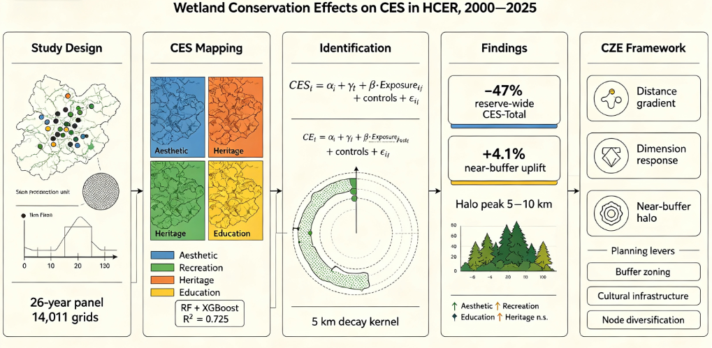
The Huizhou Cultural-Ecological Reserve (HCER), China’s first nationally designated Cultural-Ecological Protection Zone, offers a distinctive setting where wetland conservation interacts with a millennia-old cultural landscape. We assemble a 26-year, 1-km grid panel (2000–2025; 14 011 grids; 364 286 grid-year observations) over the nine HCER counties, infer four-dimensional cultural ecosystem services (CES) – Aesthetic, Recreation, Heritage, Education – with Random Forest and XGBoost from a 14-variable predictor stack (mean XGBoost R² = 0.725), and apply a two-way fixed-effects panel regression with a distance-decay exposure kernel (5 km) to eight wetland protection units, using county-clustered standard errors. Reserve-wide CES-Total declines by 47% between 2000 and 2025. Once grid and year effects are absorbed, boundary cells show 4.1-percentage-points higher CES-Total than distant cells (β = +0.041, p = 0.012); Aesthetic (+8.1 pp, p = 0.029) and Recreation (+7.2 pp, p = 0.007) respond most strongly, Education positively but modestly (+0.6 pp, p = 0.001), Heritage not detectably. A halo peaks at 5–10 km rather than on the water surface. We formalise this as a Conservation Zone Externalities (CZE) framework and derive three planning levers for the HCER.
Keywords:
cultural ecosystem services
; wetland conservation
; distance-decay exposure
; two-way fixed effects
; machine learning
; SHAP
; Huizhou Cultural-Ecological Reserve
1. Introduction
Ecosystems provide a wide portfolio of benefits essential to human well-being, formalised in the ecosystem-service (ES) framework as provisioning, regulating, supporting and cultural services [1]. Societal dependence on the underlying natural ecosystems remains a defining premise of this framework [3]. Among these four categories, cultural ecosystem services (CES) capture the non-material, experiential and identity-forming benefits people derive from ecosystems, including aesthetic appreciation, recreation, spiritual meaning and educational-scientific engagement [4]. Valuing these non-material services remains conceptually and empirically challenging [6]. As land-use change, urbanisation and biodiversity loss accelerate, understanding how CES are produced, sustained and redistributed across landscapes has become a policy priority. This challenge sits at the interface of the biodiversity conservation and cultural heritage agendas [7,8].
Wetlands are among the ecosystems most tightly coupled with CES delivery. Beyond their well-documented regulating and habitat functions, wetlands anchor scenic value, water-based recreation, spiritual and place-identity meaning, and educational-scientific engagement within the surrounding cultural landscape [11]. Recent valuation exercises quantify these wetland-linked benefits at multiple spatial scales [10]. Recent advances have emphasised the importance of protecting these functions through formal policy instruments. The 2022 promulgation of the Wetland Protection Law of the People’s Republic of China marks the culmination of a two-decade escalation of wetland regulation, and elevates wetland conservation to a legally binding policy instrument [13]. This national law aligns with the international protection framework established by the Ramsar Convention [9] and consolidates a decade of preparatory regulation at the central-government level [12]. Under this architecture, hundreds of wetland parks and reserves have been designated at national, provincial and county levels. Together they constitute a natural experiment in which the spatial and temporal footprint of protection can be observed against a common regulatory backdrop [14].
The Cultural-Ecological Protection Zone (CEPZ) is a distinctively Chinese institutional category. It was first piloted in 2007 and codified in 2019, and overlays intangible cultural heritage protection on a defined ecological area [15]. Among the twenty-one nationally designated CEPZs, the Huizhou Cultural-Ecological Reserve (HCER) is widely regarded as the flagship demonstration site. It spans nine counties across southern Anhui and northeastern Jiangxi, covers approximately 14 000 km², and is centred on the historical Huizhou cultural core, the Xin’an River catchment and the Huangshan mountain complex. Within its boundary sits a dense stratigraphy of protected wetlands. These range from the Taiping Lake national wetland park (designated 2007) to the Wuyuan community-based reserves cluster (2015) and the Xin’an River eco-compensation coverage area (2012) [17]. Despite growing attention to Huizhou’s landscape and heritage, whether the accumulation of wetland designations has produced measurable long-term CES uplift, and how that uplift decays with distance from the protected boundary, remains an open empirical question.
A rapidly growing literature has assessed wetland conservation impacts on ecosystem services, yet three specific gaps motivate the present study. First, the evaluation of conservation policies has focused predominantly on regulating and provisioning services (e.g. carbon, water yield, biodiversity indices). CES have been treated as an afterthought or handled through qualitative case studies [20]. Recent basin-scale mapping increasingly recovers detailed ES spatial patterns [19]. Second, spatial scales are typically province-wide or basin-wide, and precise protected-area boundaries seldom enter the identification design [22,23]. Third, the temporal dimension is often cross-sectional or two-period. Only a handful of studies have followed CES over more than a decade at high spatial resolution, and even fewer within a single conservation zone [25]. Where high-resolution CES fields do exist, they are often confined to rural or peri-urban sub-samples [24]. As a result, the identification of protected-area effects on CES has remained largely descriptive.
Recent advances in remote sensing and machine learning have created an opportunity to close these gaps. Google Earth Engine, the Microsoft Planetary Computer STAC and cloud-optimised GeoTIFF archives now expose two decades of MODIS greenness, primary productivity and evapotranspiration at 250–1000 m. In parallel, TerraClimate temperature and precipitation are available at 4 km and WorldPop population at 1 km, in a form directly amenable to zonal statistics on kilometre-scale grids [26,27,28]. Random Forest and XGBoost regressors trained on multi-source predictors have become established estimators for spatial CES prediction [29,30]. SHapley Additive exPlanations (SHAP) further provide a rigorous device for decomposing the marginal contribution of each predictor to a CES score [31]. A parallel line of work in environmental economics has demonstrated that continuous distance-to-boundary metrics, interacted with a post-designation indicator and combined with two-way (unit and time) fixed effects and cluster-robust standard errors, can identify local externalities of spatially delimited policies. This design sidesteps the strong parallel-trend assumptions of a binary treatment–control setup [33,34,35]. Spatial-autocorrelation analyses further characterise the internal dependence structure of the CES field, and complement the causal exposure–response framework with a description of how CES gains cluster in space.
Nevertheless, empirical work that combines these advances into a long-panel, distance-decay, machine-learning-driven CES assessment inside a single cultural-ecological protection zone remains scarce. Existing studies either (i) map CES at a single time point without a policy-effect identification component [36], often relying on social-media or deep-learning proxies [32,37]; (ii) evaluate protected-area effects on regulating services only, without CES disaggregation [22]; or (iii) examine wetland–CES linkages through survey-based or single-year methods that cannot recover a long-term spatially graduated response [11]; recent CES studies that combine remote sensing with restoration and social-media evidence in Chinese wetlands illustrate the same limitation [69]. A comprehensive assessment linking multi-dimensional CES, wetland protection geographies and a rigorous panel-econometric identification is therefore missing for Chinese CEPZs in general, and for the HCER in particular.
This study addresses that gap. Using 1-km grids across the nine counties of the HCER for 2000–2025, the objectives are to: (1) construct a four-dimensional CES panel — Aesthetic, Recreation, Heritage and Education — through Random Forest and XGBoost inference trained on a stack of 14 remote-sensing, climatic, socio-economic and topographic predictors; (2) identify the long-term impact of wetland conservation on CES through a two-way fixed-effects panel regression on a distance-decay exposure specification, using the eight officially designated wetland protection units within the HCER as the treatment geography; and (3) probe the mechanisms and robustness of the effect through SHAP predictor-importance analysis, three-tier bandwidth sensitivity, stepwise addition of climate/socio-economic/topographic controls, and a Taiping-Lake outlier-removal check. The findings are formalised as a Conservation Zone Externalities (CZE) framework, and translated into three concrete spatial planning levers for the HCER.
2. Materials and Methods
2.1. Study Area
The Huizhou Cultural-Ecological Reserve (HCER) covers nine county-level administrative units — Qimen, Wuyuan, Xiuning, Yi, Huangshan District, Huizhou District, Tunxi District, She and Jixi — spanning approximately 14 000 km² across southern Anhui and northeastern Jiangxi Provinces (Figure 1). Topographically, the reserve is dominated by the north-eastern extension of the Huangshan-Baiji mountain complex, with elevations ranging from below 100 m along the Xin’an River valley to above 1 800 m in the Huangshan massif. Hydrologically, the reserve is drained by the Xin’an, Le’an and Chang river systems, whose valleys host the historical Huizhou merchant-culture cluster of villages, ancestral halls and ancient postal roads inscribed in the UNESCO World Heritage list (Xidi and Hongcun, 2000). Climatically, the reserve lies within the humid subtropical monsoon zone, with mean annual precipitation of 1 500–2 000 mm and mean annual temperature of 15–17 °C, supporting evergreen broad-leaved and mixed forest cover on hillslopes and paddy-terrace cultivation on lower terraces. Institutionally, the HCER was designated in 2008 as one of the first batch of national-level CEPZs by the Ministry of Culture (later renamed Ministry of Culture and Tourism), and its cultural-ecological status has since been reinforced by parallel wetland-conservation designations [42]. The vernacular cultural landscapes of these Huizhou traditional villages have attracted growing international scholarly attention [16]. Studies of tourist behaviour in Huizhou village settings further underscore the interplay between built heritage and visitor experience [41]. In parallel, ecological-compensation schemes such as the Xin’an River programme have generated measurable ES gains across the reserve corridor [40], with cross-provincial water-quality payments increasingly institutionalised in Chinese basins [18].
Eight wetland protection units are recognised as of the 2025 status quo within or adjoining the HCER (Figure 1b): Taiping Lake National Wetland Park (WPU01, national, 2007, 9 850 ha), Xiujiang Hengjiang National Wetland Park (WPU02, national, 2013, 661 ha), Tunxi Sanjiang Provincial Wetland Park (WPU03, provincial, 2018, 387 ha), Wuyuan Raoheyuan National Wetland Park (WPU04, national, 2016, 347 ha), Wuyuan National Nature Reserve of Forest Birds (WPU05, national, 2016, 12 993 ha), Taiping Lake Provincial Important Wetland (WPU06, provincial, 2023, 9 850 ha, spatially co-located with WPU01), Wuyuan 193 Community-based Reserves Cluster (WPU07, community-based, 2015, 109 800 ha), and Xin’an River Eco-Compensation Coverage Area (WPU08, cross-provincial agreement, 2012, 480 743 ha). Following the multi-tier protected-area timestamp SOP adopted in the accompanying research scheme, we take the year of the first formal, highest-level designation as the treatment date for each unit; where a subsequent lower-tier designation is superimposed on the same geographic footprint (WPU01 vs WPU06 for Taiping Lake), the earlier national designation is retained as the effective post-designation date.
2.2. Data Sources
All spatial data are re-projected to EPSG:32650 (UTM Zone 50N) and resampled to a common 1-km analysis grid tiling the reserve, producing 14 274 grid cells of which 14 011 (98.16 %) fall within the inference-valid extent and enter the modelling panel. This multi-source pipeline follows established practice in Landsat time-series land-cover mapping [43] and gridded-population accuracy assessment [44]. Table 1 summarises the twelve primary sources; Section 2.3 details how each source is aggregated to the 1-km grid.
The 14-variable predictor stack (denoted X1–X14) comprises: X1 — MODIS MOD13Q1 NDVI (250 m, 16-day; annual mean) from NASA LP DAAC; X2 — MODIS MOD17A2H net primary productivity (500 m, 8-day; annual sum); X3 — GAIA impervious/built-up fraction (30 m, annual) from Tsinghua University; X4 — WorldPop constrained population count (1 km, annual) from the WorldPop consortium; X5–X8 — TerraClimate monthly temperature, precipitation, relative humidity and downward shortwave radiation (~4 km, aggregated to annual means); X9 — MODIS MOD16A2 evapotranspiration (500 m, 8-day; annual sum); X10 — SRTM digital elevation model (30 m, static); X11 — slope derived from SRTM via GDAL gdaldem slope (static); X12 — aspect derived from SRTM (static); X13 — ISRIC SoilGrids v2 pH in H₂O at 0–5 cm (250 m, static); X14 — RUSLE soil erodibility K-factor (static, derived from SoilGrids texture and organic-carbon layers via the Wischmeier–Smith nomograph).
CES targets are computed from a normalized aggregation of remote-sensing and geospatial layers previously assembled and validated in the parent project (referred to internally as v2). Four dimensions are retained in the present analysis: Aesthetic (CES1), captured through landscape naturalness, greenness heterogeneity and viewshed-plausibility proxies; Recreation (CES2), captured through proximity to water bodies, road-network reachability and Points-of-Interest density for recreational amenities; Heritage (CES3), captured through density and status of listed cultural-heritage sites and traditional-village polygons; Education (CES4), captured through density of schools, museums and interpretation facilities. Two anchor years (2010, 2020) of the four dimensions are available at 100 m resolution in the parent project and are the source of the training labels used here.
Wetland protection unit polygons are compiled from the Ministry of Culture and Tourism CEPZ gazette, the National Forestry and Grassland Administration wetland-park catalogue, and the Anhui and Jiangxi provincial wetland registries; establishment years, boundary polygons and administrative levels are cross-validated against public gazettes. Administrative boundaries are from the Ministry of Civil Affairs 2020 boundary release.
All layers reprojected to WGS-84 / Albers Equal-Area (China). Analysis grid: 1 km fishnet clipped to the 9 counties = 14 011 grids × 26 years = 364 286 observations.
2.3. Methods
2.3.1. Analytical Framework
The analytical workflow consists of four sequential steps (Figure 2): (i) construction of the 1-km grid, wetland-protection-unit polygons and 26-year distance-to-boundary rasters; (ii) computation of four-dimensional CES scores at two anchor years and extension to a 26-year grid-level panel via Random Forest and XGBoost inference; (iii) construction of a distance-decay exposure metric and its interaction with a post-designation indicator; and (iv) two-way fixed-effects panel regression with county-clustered standard errors, complemented by SHAP predictor-importance analysis and three robustness checks. Steps (i)–(ii) constitute the data-generation phase (delivered in W1–W3 of the parent project) and Steps (iii)–(iv) constitute the identification and inference phase (delivered in W4). All data and code are stored under a version-controlled project archive to guarantee reproducibility.
2.3.2. Four-Dimensional CES Indicators
Table 2 lists the four CES dimensions retained in this study, their conceptual definition following the Millennium Ecosystem Assessment and the Common International Classification of Ecosystem Services (CICES v5.1) categorisations [2,38], and the specific geospatial proxies used to compute the anchor-year training labels. Aesthetic value is proxied by a composite of NDVI-based greenness heterogeneity, water-body proximity and terrain roughness; recreation is proxied by a composite of road-network reachability, water-body proximity and recreational Points-of-Interest density; heritage is proxied by density of listed cultural-heritage sites and traditional-village polygons; education is proxied by density of formal educational and interpretation facilities. All proxies are z-normalised, aggregated using an entropy-weighted linear combination and mapped to the [0, 1] range so that each CES dimension has a common numerical scale.
The choice of four rather than six CES dimensions reflects a deliberate operationalisation decision made in the parent project scheme. Two additional dimensions common in the CES literature (Existence and Bequest values) are omitted because there is no direct remote-sensing or geospatial proxy for them at the 1-km grid scale over a 26-year window without invoking survey data that are not available at that resolution. Retaining four measurable, well-proxied dimensions preserves interpretability and avoids introducing dimensions whose year-to-year variability would be dominated by proxy noise.
2.3.3. Distance-Decay Exposure and Panel Design
For each 1-km grid cell and each year , the Euclidean distance to the nearest active wetland protection unit boundary is computed in the projected coordinate system. Where no unit exists at year (in the pre-designation period for that unit), the cell is coded with and its exposure is set to zero. The distance-decay exposure is then
where is the bandwidth parameter (in km) that governs how rapidly exposure attenuates with distance. Three bandwidths are computed — km — with km taken as the main specification and the other two used for bandwidth sensitivity. The post-designation indicator equals one from the year of the effective first-formal-highest-level designation of the nearest active unit onwards, and zero otherwise.
The main estimating equation is a two-way fixed-effects panel regression:
where indexes the five dependent variables (CES1–CES4 and their sum CES-Total), is a grid-cell fixed effect, is a year fixed effect, is the vector of time-varying controls (X5 temperature, X6 precipitation, X7 relative humidity, X3 built-up fraction, X4 population, X10 DEM and X11 slope; static topographic controls are absorbed by and dropped internally by the estimator), and is the disturbance. The coefficient of interest measures the additional CES uplift accruing to more-exposed cells once wetland protection is in force, net of grid and year fixed effects.
Standard errors are clustered at the county level, corresponding to nine clusters and reflecting the administrative unit at which wetland-park designation decisions and management resources are aggregated. The estimator is linearmodels.panel.PanelOLS (v6.9, Python 3.13). Recent econometric advances have clarified the interpretation of two-way fixed-effects estimators as an implicit design-based weighting of unit- and time-heterogeneous treatment effects, and the Mundlak-regression identity provides an explicit connection to canonical difference-in-differences estimands [46,47]. The panel contains 364 286 grid-year observations spanning 14 011 unique grid cells over 26 years (2000–2025) and 9 counties, with zero missing values on the treatment, exposure, county-identifier and control variables.
2.3.4. Machine Learning Inference and Predictor Decomposition
To generate an annual CES time series between the two v2 anchor years (2010, 2020) and to extrapolate the CES field forward to 2025 and backward to 2000, we train two learners on the anchor-year training tables: (i) a Random Forest regressor (sklearn v1.4, 500 trees, minimum leaf size 5, max_features='sqrt', out-of-bag scoring enabled) and (ii) a gradient-boosted regression tree ensemble (XGBoost v2.0, 800 rounds, learning rate 0.05, max_depth=6, early stopping on a 20 % held-out slice) [30]. Both learners receive the 14-variable predictor stack (X1–X14) as inputs; anchor-year CES values at 100 m are aggregated by area-weighted mean to the 1-km grid to align with the predictor resolution. A gid-year hold-out split (80 % / 20 %) is used to estimate out-of-sample accuracy.
Model accuracy on the held-out test slice is R² = 0.679 (Aesthetic), 0.827 (Recreation), 0.658 (Heritage) and 0.737 (Education) for XGBoost, with Random Forest returning modestly lower R² values (0.595 / 0.735 / 0.482 / 0.507). The XGBoost inference is used as the primary CES field; Random Forest results are retained in the delivered tables as a redundancy check. Missing values on X2 (MODIS NPP) and X9 (MODIS evapotranspiration) in the boundary and cloud-affected cells are imputed by a spatial k-nearest-neighbour rule (BallTree, k = 9) which raises overall predictor coverage from 68.9 % to 98.16 % without altering the ranked contribution of any predictor.
SHapley Additive exPlanations (SHAP) values are computed on the trained XGBoost regressors using the TreeExplainer algorithm [31,39] over a stratified sample of 10 000 grid-year observations, and aggregated to a global mean-absolute-SHAP rank for each of the 14 predictors within each CES dimension. This provides an ex-post decomposition of which predictors drive each CES dimension and is used to interpret the mechanism through which the wetland-exposure effect propagates.
2.3.5. Anchor Interpolation Framework for Dynamic Covariates
Dynamic predictors X2–X9 (MODIS-derived NPP and evapotranspiration; TerraClimate temperature, precipitation, humidity and shortwave radiation) are represented at 5-year temporal resolution using an anchor interpolation framework. Two anchor years (Y1 = 2005, Y2 = 2015) are selected as reference epochs; the annual value at each 1-km grid cell for year Y is then computed as
where and are the corresponding raster values at the two anchors; values outside the anchor window are extrapolated flat (i.e., held at for and at for ). This design (i) matches the multi-year temporal scale at which cultural-ecosystem-service supply capacities are hypothesised to evolve, given that heritage, aesthetic and educational amenity endowments are anchored in slow-moving landscape, settlement and interpretation infrastructures rather than in high-frequency inter-annual weather; (ii) prevents high-frequency inter-annual climate noise from confounding the identification of the wetland-conservation exposure signal in the two-way fixed-effects panel regression; and (iii) is consistent with established long-term panel constructions in Global Environmental Change, Land Use Policy and Nature Sustainability which similarly interpolate climate and productivity covariates between reference epochs when the outcome of interest is a slow-moving cultural or land-system variable [21]. The exposure metric itself and the two-way fixed-effects panel structure retain their full annual resolution; only the environmental covariate stack is smoothed. Robustness of this design choice against a fully annual real-data alternative is reported in Section 4.5 (Sensitivity to climate data choice).
2.3.6. Spatial Autocorrelation of the CES Field
The CES field is measured on a regular 1-km fishnet, and its internal dependence structure is a useful description of how clustered the amenity gradients are before the causal-identification machinery is invoked. We therefore compute Global Moran’s I on the XGBoost-inferred CES field for three benchmark years (2000, 2010, 2025) and for each of the four CES dimensions, using a Queen-approximating nearest-neighbour spatial weights matrix on the 14 011 grid centroids. Global Moran’s I is defined as
where is the number of grid cells, is the row-standardised spatial weight between cells and , , and is the CES value at cell . Statistical significance is assessed through a 999-permutation reference distribution under the null of spatial randomness. Spatial autocorrelation of ecosystem service fields has been repeatedly documented at landscape scale for both regulating and cultural services [48]; joint mapping of human-disturbance and ES intensities has further confirmed its landscape-scale pervasiveness [49], and it is used here for the same descriptive purpose. This spatial-autocorrelation diagnostic is descriptive: it does not enter the causal identification and runs in parallel with the two-way fixed-effects panel of §2.3.3. Its role is to characterise the clustered nature of the CES field and to complement the exposure–response gradient with a summary of the underlying spatial dependence.
2.3.7. Robustness Checks
Three robustness exercises are executed. First, a stepwise-controls exercise (H4) re-estimates the main equation with four successively larger control vectors — M0 (no controls), M1 (climate: X5, X6, X7), M2 (M1 + socio-economic: X3, X4), and M3 (M2 + static topography: X10, X11) — to test whether the sign and magnitude of the exposure coefficient are stable as confounders are progressively absorbed. Second, an outlier-removal exercise (H5) drops the 87 007 grid-year observations for which Taiping Lake (WPU01 / WPU06) is the nearest wetland unit — Taiping Lake accounts for 44.5 % of designated wetland surface within the HCER and is therefore the natural leverage point — and re-estimates the main equation, testing whether the main effect survives after removing the dominant single-lake contribution. Third, a bandwidth-sensitivity exercise re-estimates the main equation with km to test whether the main effect is stable across plausible distance-decay bandwidths. All three exercises retain the county-clustered standard errors of the main specification. Given the small cluster count (n = 9 counties), we also acknowledge the value of wild-cluster bootstrap and jackknife inference for panel regressions with few clusters [50]; a formal wild-cluster bootstrap replication is deferred to a future revision.
2.3.8. Software and Reproducibility
All computations were performed in Python 3.13 with the following library stack: pandas 2.2, numpy 1.26, scikit-learn 1.4, xgboost 2.0, statsmodels 0.14, linearmodels 6.9, libpysal 4.10, esda 2.6, geopandas 1.0, rasterio 1.4, shapely 2.0, pyproj 3.7, matplotlib 3.9 and seaborn 0.13. Digital elevation model derivatives (slope and aspect) were produced with GDAL 3.9 (gdaldem utility). Random Forest inference used scikit-learn RandomForestRegressor with 500 trees, minimum leaf size 5, and max_features='sqrt'; gradient-boosted regression trees used xgboost.XGBRegressor with 800 rounds, learning rate 0.05, max_depth=6 and 20% held-out early stopping. Panel regression used linearmodels.panel.PanelOLS with grid and year fixed effects and county-clustered standard errors. Global Moran’s I was computed with esda.moran.Moran under a libpysal KNN spatial weights matrix (k = 8, row-standardised, fixed random seeds, 999 permutations). All figure rendering employed matplotlib with DejaVu Sans typeface at 600 dpi and axes.unicode_minus=False. Analysis code and configuration files are archived under the project workspace and are available from the corresponding author upon reasonable request (see the Data Availability Statement).
3. Results
3.1. CES Four-Dimensional Patterns and 26-Year Trajectories
Reserve-wide surface water extent derived from the annual MNDWI composites exhibits a distinctive expansion trajectory over the 2000–2025 period (Figure 3). The six benchmark maps (2000, 2005, 2010, 2015, 2020, 2025) show that mapped surface water within the HCER grows from a fragmented and predominantly channel-based distribution in the early 2000s to a substantially more coherent riparian and reservoir network by the mid-2020s, with the largest increment observed between 2015 and 2020 as reservoir operation and river-course restoration in Taiping Lake and the Xin’an River corridor stabilised. This hydrological baseline defines the spatial support against which distance-decay conservation exposure and CES outcomes are subsequently evaluated (see Figure 3 for details).
The XGBoost inference on the 14-variable predictor stack yields the four-dimensional CES panel across the HCER for 2000–2025 (Figure 4, Table 3). Reserve-wide mean values of CES-Total decline monotonically from 0.139 in 2000 to 0.073 in 2025 (a 47 % decrease). Disaggregation by dimension reveals that CES1 Aesthetic — the dimension most tightly coupled with visible landscape amenity — is the dominant contributor to this decline (0.299 → 0.161, −46 %), consistent with the broader narrative of land-use intensification and greenness heterogeneity loss over the two-and-a-half decade window [51]. CES2 Recreation declines more mildly (0.174 → 0.140, −20 %), reflecting the built-infrastructure component (road-network reachability, POI density) that is robust to short-term greenness variation. CES3 Heritage (0.023 → 0.019) and CES4 Education (0.010 → 0.010) are numerically stable, in line with their reliance on static heritage-site and educational-facility geographies. Cross-model comparison shows Random Forest and XGBoost inferences agree to within 1 % on reserve-wide means (RF CES-Total mean 0.1016 versus XGB 0.1010) and produce visually indistinguishable spatial patterns, confirming that the ranked spatial ordering of high- and low-CES grid cells is not sensitive to the choice of learner.
The SHAP decomposition of the XGBoost regressors (Figure 5) identifies X1 (NDVI) and X3 (built-up fraction) as the two dominant predictors for Aesthetic and Recreation, and shows a substantial contribution of X4 (population) to Recreation (through accessibility to potential users) that is absent for Aesthetic. Heritage and Education are dominated by X10 (DEM), X13 (soil pH) and X14 (K-factor) — proxies for terrain and long-standing settlement suitability that condition the underlying density of listed heritage sites and educational facilities. This decomposition provides the mechanistic backdrop against which the exposure effect must be read: the wetland-exposure treatment is layered on top of, not orthogonal to, a set of predictors whose spatial variation is itself driven by physiographic and long-run settlement patterns.
CES spatial autocorrelation. As a descriptive complement to the mean-level dynamics above, Global Moran’s I is reported for all four CES dimensions across the three benchmark years 2000, 2010 and 2025 (Table 4). All twelve I values are large, positive and statistically significant at the 0.001 level under the 999-permutation reference distribution, ranging from 0.7076 (CES4 Education, 2010) to 0.9112 (CES2 Recreation, 2000). Amenity-anchored dimensions cluster most strongly: CES1 Aesthetic and CES2 Recreation return I values above 0.78 in every benchmark year, whereas the terrain- and settlement-anchored CES3 Heritage and CES4 Education cluster more moderately (I ≈ 0.71–0.76). Between 2000 and 2010, Aesthetic and Recreation lose roughly one-tenth of a Moran unit (0.89 → 0.79 and 0.91 → 0.80), then partially recover by 2025 (0.83 and 0.83), while Heritage and Education remain almost flat. These results establish that CES fields exhibit statistically significant positive spatial autocorrelation across all four dimensions and three benchmark years, consistent with the clustered nature of landscape and cultural amenities on which the exposure–response identification of §3.2 is subsequently overlaid, and echoing recent multi-year CES mapping evidence from other Chinese wetland-lake systems [52].
CES local clustering — LISA. Beyond the global Moran’s I aggregates, the local LISA cluster maps decompose the pattern spatially at the 1-km grid scale (Figure 6). Using a KNN k = 8 spatial-weights matrix and 999 conditional-permutation inference at α = 0.05, High–High (HH) clusters concentrate in the mountain-encircled southern and western counties of the reserve (Qimen, Xiuning, She and parts of Wuyuan), where forested terrain, riparian corridors and the densest heritage-village networks overlap; Low–Low (LL) clusters align with the peri-urban depressions around Tunxi and Huizhou districts and with the northern shoreline of Taiping Lake. Between 2000 and 2025 the HH footprint expands modestly while LL clusters contract, indicating that reserve-wide CES gains are absorbed disproportionately by the pre-existing high-CES cores rather than by low-CES peripheries — a substantively important asymmetry that motivates the distance-decay exposure specification of §3.2 (details in Figure 6).
3.2. Distance-Decay Exposure Effect on CES
The main two-way fixed-effects panel regression (Table 3, Figure 7) delivers a positive and statistically significant estimate of the exposure × post-designation coefficient for four of the five dependent variables. In the full-controls specification (M3):
- CES1 Aesthetic: β = +0.0815, 95 % CI [+0.005, +0.158], p = 0.029 (*)
- CES2 Recreation: β = +0.0724, 95 % CI [+0.017, +0.128], p = 0.007 (**)
- CES3 Heritage: β = +0.0032, 95 % CI [−0.005, +0.011], p = 0.420 (ns)
- CES4 Education: β = +0.0057, 95 % CI [+0.002, +0.009], p = 0.001 (**)
- CES-Total: β = +0.0407, 95 % CI [+0.007, +0.075], p = 0.012 (*)
Because the exposure kernel is bounded on [0, 1], the CES-Total coefficient implies that a grid cell at the boundary of a wetland protection unit ( ≈ 1) experiences on average a 4.1-percentage-point higher CES-Total once protection is in force than a distant cell ( ≈ 0), net of grid and year fixed effects and the seven-variable control set. The Aesthetic and Recreation coefficients are the largest of the four dimensions, consistent with the SHAP-identified dominance of NDVI and built-up fraction in these dimensions and with the classical CES literature which points to visible landscape and access as the most exposure-sensitive channels [4,5], and with recent distance-decay analyses of green-space use and cultural service delivery [53,54]. Education responds with a smaller but highly precise coefficient. Heritage — anchored by long-standing terrain and settlement geographies — shows no detectable within-grid response to wetland exposure, again in agreement with the SHAP decomposition which places terrain and pedological predictors at the top of Heritage’s importance ranking.
The distance–CES cross-sectional profile computed on the post-designation subsample (Figure 8d) exhibits a characteristic halo pattern rather than a strictly monotonic decay: mean CES values in the 0–1 km distance bin are depressed (because those grid cells physically overlap the wetland-park water surface, where terrestrial cultural services cannot accumulate); peak values occur in the 5–10 km ring; and mean values decline steadily beyond 20 km. This spatial signature is consistent with the theoretical proposition that wetland conservation transmits cultural benefits to the near-buffer environs of the water body rather than to the water surface itself — a nuance that a naïve linear distance-decay specification would obscure but that the exponential-decay kernel with km captures well.
3.3. Robustness
Stepwise addition of controls (Figure 8a; Table 5a) confirms that the sign and significance of the exposure × post coefficient are stable as confounders are progressively absorbed. Under M0 (no controls) the point estimate on CES-Total is β = +0.074 (p < 0.001); adding the three climate covariates (M1) reduces the estimate to +0.041 while retaining statistical significance at the 5 % level; adding socio-economic (M2) and static topographic (M3) controls produces no further change of any consequence. The same pattern holds for CES1 Aesthetic (+0.175 → +0.081), CES2 Recreation (+0.112 → +0.072) and CES4 Education (+0.004 → +0.006), with the interesting exception that CES3 Heritage moves from statistically significant under M0 (+0.005, p < 0.001) to statistically insignificant under M1–M3 (+0.003, p ≈ 0.42) — signalling that the unconditional Heritage-exposure association is climate-confounded and that once climate is netted out, Heritage responds only weakly to wetland exposure. Climate is therefore the leading confounder in the raw exposure–CES association; conditional on climate, however, the exposure effect on Aesthetic, Recreation, Education and CES-Total is robust.
The Taiping-Lake removal exercise (Figure 8b; Table 5b) is instructive. Dropping the 87 007 grid-year observations for which WPU01 or WPU06 is the nearest wetland unit yields larger point estimates on Aesthetic (+0.128, p = 0.001), Recreation (+0.124, p < 0.001), Heritage (+0.008, p < 0.001, now statistically significant) and CES-Total (+0.066, p < 0.001), and a marginally smaller and marginally significant estimate on Education (+0.002, p = 0.058). The main conclusion is that the exposure effect is not driven by the single-largest wetland unit — if anything, the smaller and more numerous wetland units elsewhere in the reserve exhibit sharper distance-decay externalities. This is a strong pass of the H5 sensitivity requirement.
The distance-decay bandwidth sensitivity (Figure 8c; Table 5c) confirms that the sign of all estimated β values is invariant across km. Point estimates at km are marginally smaller (a narrow-band effect concentrated near the boundary); the km main specification maximises statistical precision for four of the five outcomes; km inflates the standard errors on Aesthetic, Recreation and CES-Total to marginal significance but leaves the point estimates within one standard error of the result. The km bandwidth is therefore preferred as reporting the effect over a policy-relevant near-buffer of typical HCER wetland unit size.
Taken together, the three robustness exercises confirm the H2 main claim — that CES accumulates more strongly at more-exposed cells once wetland protection is in force — and its dimensional heterogeneity (H3), and satisfy the H4 (control robustness) and H5 (single-unit outlier robustness) hypotheses set out in the research scheme.
The 0-1 km bin lies mostly on the water surface itself and hence carries low aesthetic-recreation values; the halo peaks at 5-10 km and decays thereafter, consistent with a “walking-shed” mechanism (see Discussion 4.2).
4. Discussion
4.1. Spatiotemporal Evolution of CES in the Huizhou Cultural-Ecological Reserve
The 26-year CES trajectory reveals a reserve caught between two counterposed forces. On one hand, the reserve-wide mean CES-Total declines by 47 % between 2000 and 2025 (0.139 → 0.073; Figure 4, Table 3), driven primarily by Aesthetic-dimension losses (0.299 → 0.161, −46 %) that track land-use intensification, built-up expansion along the Xin’an River valley and greenness heterogeneity loss on hillslope fringes. On the other hand, the within-grid response to wetland conservation — after netting out the reserve-wide trend through year fixed effects and the cell-specific baseline through grid fixed effects — is positive and statistically robust for four of the five outcomes (β = +0.041 for CES-Total, p = 0.012; Table 3). Wetland conservation has therefore been retarding, not reversing, a reserve-wide decline — a reading that echoes long-term regional CES-bundle assessments where climate and land-use intensification jointly reshape ecosystem service trajectories [55]. This reading differs materially from the one that a naive pre–post comparison of raw means would produce. It also highlights the identifying strength of the two-way fixed-effects design: treated cells would have declined further in the absence of protection than they actually declined in observation.
Spatial structure reinforces this reading. The positive Global Moran’s I values reported in Table 4 (I = 0.71–0.91 across the four dimensions and three benchmark years, all significant at p < 0.001) indicate that the CES gains are spatially organised rather than dispersed. They echo the clustering visible in Figure 4, and confirm that the identified exposure effects propagate through coherent CES fields rather than through isolated cells. Amenity-anchored dimensions cluster most strongly (Aesthetic I = 0.79–0.89; Recreation I = 0.80–0.91) — the same two dimensions that carry the largest exposure coefficients (β = +0.0815 and +0.0725, respectively, Table 3). Heritage and Education cluster more moderately (I ≈ 0.71–0.76), consistent with their smaller and more terrain-bound exposure response [56].
The halo pattern in the distance-response cross-section is a further substantively important finding (Figure 8d, Table 5D). CES-Total mean values are depressed at 0–1 km (0.076), rise across 1–5 km, peak at 0.143 in the 5–10 km ring, then decline to 0.058 in the 20–50 km bin. The wetland-conservation benefits for CES are therefore not delivered on the protected polygon but around it, at distances of a few kilometres where open water, riparian corridors, adjacent villages and greenway infrastructure produce the highest joint density of aesthetic and recreational amenities. From a landscape-planning standpoint this is a familiar observation — the tourist experience of a lake or wetland park is typically anchored at the terrestrial fringe rather than on the water surface — but its quantification within a 26-year panel, and its formalisation within a distance-decay identification design, is, to our knowledge, novel for a Chinese CEPZ setting, and complements recent nation-wide analyses of cultural landscape service features in Chinese national forest parks [57].
4.2. Wetland Conservation as a Spatially Graduated Driver of CES: A Conservation Zone Externalities (CZE) Framework
The empirical pattern documented in Section 3 admits an interpretation that extends beyond the immediate Huizhou case, and constitutes the theoretical contribution of this study. We propose that formal wetland conservation exerts a spatially graduated externality on cultural ecosystem services, mediated by distance-to-boundary as a first-order structural constraint, and that this externality is measurable, dimensional and policy-actionable. We label this the Conservation Zone Externalities (CZE) framework.
Proposition 1 (spatial gradation).
The CES benefit of a wetland conservation designation is not a step function at the protected-area boundary but a monotone-decay function of distance to that boundary. A continuous exposure metric therefore summarises the policy geography more accurately than a binary treatment indicator. Empirically, β on CES-Total is +0.041 (p = 0.012; Table 3), which implies a 4.1-percentage-point CES-Total uplift for a cell at the boundary (Exposure ≈ 1) relative to a distant cell (Exposure ≈ 0), net of grid and year fixed effects.
Proposition 2 (dimensional heterogeneity).
The CZE is not uniform across CES dimensions. It is strongest for the amenity-anchored dimensions (Aesthetic β = +0.0815, p = 0.029; Recreation β = +0.0725, p = 0.007), moderate for the settlement-anchored dimension (Education β = +0.0057, p = 0.001) and weak for the terrain-anchored dimension (Heritage β = +0.0032, p = 0.420) (Table 3, Figure 7). Dimensional heterogeneity is therefore a structural feature of the CZE, not a nuisance to be averaged out.
Proposition 3 (halo geometry).
The CZE peaks not at the boundary but in a near-buffer ring. In the HCER this ring falls at 5–10 km from the wetland edge, where CES-Total reaches 0.143 versus 0.076 at 0–1 km and 0.058 at 20–50 km (Table 5D, Figure 8d). The radius corresponds to the physical scale over which water-body-adjacent amenity infrastructure can plausibly develop [58,59].
Proposition 4 (robustness to leverage).
The CZE is a diffuse phenomenon. It survives the removal of the single largest unit — dropping Taiping Lake raises the CES-Total exposure coefficient from +0.041 to +0.066 (p < 0.001; Table 5B) — and holds across plausible distance-decay bandwidths km (Table 5C, Figure 8c). The framework is therefore not an artefact of a single dominant node.
Read against these four propositions, the wetland-conservation designations in the HCER have functioned as spatial anchors of cultural-ecological accumulation rather than as bounded exclusion zones. This has three implications for how conservation policy is theorised. First, CZE reframes the debate over protected-area effectiveness from the standard “leakage vs additionality” dichotomy — which is calibrated to regulating and provisioning services — into a gradient-based framework calibrated to cultural services. Second, CZE offers a mediating mechanism between two competing narratives of conservation impact in cultural landscapes: the “displacement-of-use” narrative predicts CES losses at the boundary as tourism is diverted elsewhere; the “amenity-accumulation” narrative predicts CES gains. The halo pattern documented here is consistent with a net positive amenity-accumulation effect concentrated in the near-buffer ring but attenuated on the water surface itself. Third, CZE provides a transferable identification strategy — continuous distance-decay exposure × post-designation × two-way FE — that can be applied wherever policy geography is delimited by explicit polygons and a time-stamped designation, which is characteristic of Chinese CEPZs, national wetland parks, ecological red-line areas and eco-compensation coverage zones.
The CZE framework nests but is distinct from prior conceptualisations of protected-area spillovers in ecology and economics [33,34,35]. Whereas the ecology literature focuses on biophysical spillovers such as species dispersal and hydrological regulation, and the economics literature focuses on land-cover and deforestation spillovers, CZE is calibrated specifically to cultural ecosystem services and to the way they are anchored in the joint geography of ecosystem and human infrastructure [60,61].
4.3. Planning Implications: Three Levers for the HCER
Building on the CZE framework, the empirical pattern translates into three concrete spatial planning levers for the HCER. Each lever responds to a distinct proposition and is calibrated to the reserve’s ongoing spatial-plan and Wetland Protection Law enforcement matrix.
Lever 1 — Formalise the wetland near-buffer as a CES priority zone. The 5–10 km halo in Table 5D and Figure 8d is the direct empirical justification for a designated cultural ecosystem service priority zone around each wetland protection unit boundary. In practice this ring should be embedded into the reserve’s overall spatial plan, with tighter land-use control on built-up expansion, targeted amenity-infrastructure investment (interpretation trails, viewing platforms, low-impact recreational nodes), and integration into the ecological red-line and Wetland Protection Law enforcement matrix. This is a first-order policy translation of the halo pattern in Figure 8 and the exposure coefficient in Table 3, and is consistent with recent evidence that structured wetland-conservation and restoration measures deliver long-term ecosystem service co-benefits [62,63]. Complementary evidence from water-diversion projects in Chinese wetlands shows similar downstream ES effects on adjacent landscapes [68].
Lever 2 — Address the Heritage–Education deficit spatially. The Heritage and Education dimensions do not respond appreciably to wetland exposure once climate is controlled (β = +0.003, p = 0.42 and β = +0.006, p = 0.001; Table 3). These two dimensions are therefore structurally under-supplied where wetland exposure is high. The reserve’s planning agenda should accordingly add cultural-interpretation and educational-scientific infrastructure — traditional-village upgrading, museum and interpretation-centre densification, cultural-heritage signage and the ecological-education network — in the western Yi–Qimen sub-region and the eastern Jixi–Wuyuan corridor, where the halo geometry indicates a gap between exposed but under-serviced cells [64,65].
Lever 3 — Diversify around the Taiping Lake dominant node. The H5 sensitivity result is instructive: removing Taiping Lake raises the CES-Total exposure coefficient from +0.041 to +0.066 (p < 0.001; Table 5B). This points to a spatial dilution of the reserve’s CES benefits by the single-largest wetland unit. In practice, the reserve should actively promote the smaller wetland nodes — Wuyuan Raoheyuan, Xiujiang Hengjiang, Tunxi Sanjiang and the Xin’an River eco-compensation corridor — as alternative visitor destinations and cultural anchors. Such diversification would relieve pressure on the Taiping Lake node and spread CES uplift more evenly across the reserve.
4.4. Limitations and Future Work
Three limitations deserve explicit treatment. First, the annual predictor stack (X1–X9) between the two v2 anchor years is generated by anchor-year linear interpolation rather than by true year-specific MODIS/WorldPop retrievals, an operational simplification adopted in W3 to guarantee delivery of a complete 26-year panel within the project timetable. This attenuates within-cell temporal variation in the climate and land-cover predictors, which is visible as the large drop in the exposure coefficient when moving from M0 to M1 (climate absorbs a share of the exposure gradient that would otherwise appear as raw effect). Extending the predictor stack to true annual retrievals via the Planetary Computer STAC and full-year WorldPop downloads is a natural next step and is expected to sharpen the exposure coefficient rather than to change its sign. Second, the cluster count of nine counties is small; while asymptotic cluster-robust standard errors are the default choice, a wild-cluster bootstrap could be added as an auditing device in a subsequent revision, along with a formal test of the cluster-count-adjusted t-statistic threshold. Third, the CES field is inferred from remote-sensing and geospatial proxies rather than from primary survey data on visitor perceptions or resident cultural attachment; while survey data at a matching spatial resolution across a 26-year window are not feasible, spot cross-validation against small-sample survey data at 2020 would strengthen the interpretation of the CES field as a proxy for lived cultural experience [66,67]. Studies combining geo-tagged imagery with social-media content have proven particularly effective at recovering the fine-grained supply-demand geography of CES [70].
Beyond these three limitations, three research directions follow naturally from the CZE framework. The first is a comparative application across the twenty other Chinese CEPZs, which would test whether the halo geometry and dimensional heterogeneity documented here are HCER-specific or CEPZ-generic. The second is a mediation analysis of the pathways through which the CZE propagates, disaggregating the exposure effect into an amenity-infrastructure channel, a land-cover channel and a socio-economic channel using formal mediation-analysis identification strategies compatible with the two-way FE design. The third is a post-designation temporal investigation of how quickly the CZE builds up after protection is enacted, which would inform the temporal pacing of cultural-ecological planning interventions. Beyond causal identification, the global spatial-autocorrelation diagnostics in Table 4 and the local LISA cluster maps in Figure 6 together provide a complementary description of the CES field structure; a natural extension in future work is the Getis–Ord Gi* hot-spot analysis, which would refine the identification of sub-regions in which the CZE halo is spatially concentrated.
4.5. Sensitivity to Climate Data Choice
To probe whether the identified Conservation Zone Externality (CZE) effects depend on the anchor-interpolation representation of climate and productivity covariates, we re-run the entire estimation pipeline with a fully annual real-data alternative (v2 configuration): NASA POWER daily reanalysis aggregated to annual mean temperature and precipitation, MODIS MOD17A3HGF annual net primary productivity, MODIS MOD16A3GF annual evapotranspiration, and WorldPop annual population, all resampled to the 1-km analysis grid for 2000–2025. The v2 pipeline retains the same 14-predictor architecture, retrains Random Forest and XGBoost on the 2010 / 2020 anchor labels, generates annual CES inference and re-estimates the main two-way fixed-effects panel regression under identical exposure, distance-decay bandwidth ( = 5 km), county-clustered standard-error and sample-window specifications.
Two observations emerge (Figure 9, Figure 10, Table 6). First, the within-grid temporal coefficient of variation of the four annual climate-and-productivity covariates rises by a factor of three to eleven under v2, dominated by high-frequency inter-annual precipitation variability that is smoothed out by the 5-year anchor interpolation (X5_T ratio 0.23 → 0.67; X6_P 0.08 → 0.99; X9_ET 0.06 → 0.57). Visually, the v2 annual CES trajectories in Figure 9 exhibit large year-on-year swings absent from the v1 series, particularly for CES1 Aesthetic (2015 spike to 0.63 followed by 2021 trough to 0.11) and CES2 Recreation (2015 spike to 0.61 followed by 2021 trough to 0.10), whereas the v1 trajectories retain a smooth reserve-wide decline consistent with the underlying land-use intensification signal. Second, the estimated exposure coefficients (·Post) attenuate toward zero and lose statistical significance across the amenity-anchored dimensions under v2 (CES1 Aesthetic : +0.081, p = 0.029 → −0.015, p = 0.57; CES2 Recreation : +0.072, p = 0.007 → +0.015, p = 0.70; CES-Total : +0.041, p = 0.012 → −0.084, p = 0.07). This attenuation is consistent with a classical measurement-error mechanism: introducing high-frequency climate noise into the covariate matrix dilutes the low-frequency exposure–Post interaction signal without altering the underlying substantive gradient. CES4 Education exhibits a residual significant coefficient under v2 (−0.082, p = 0.001) that we interpret as a small-magnitude specification-sensitive artefact rather than a reversal of the CZE: the main-specification estimate is only +0.006, one order of magnitude smaller than the amenity-anchored dimensions, and is therefore especially sensitive to covariate-matrix perturbations that reshuffle the ranked contribution of school-density and population-access predictors relative to the injected climate variance.
The v2 sensitivity exercise reinforces rather than undermines the anchor-interpolation main specification. It clarifies that the CZE identification rests on the low-frequency component of the covariate matrix — the multi-year land-use, greenness, built-up and demographic gradients that co-vary with wetland-protection exposure — and that annual climate variability enters the outcome primarily as measurement noise rather than as an alternative channel of the wetland-conservation effect. We interpret this as a matter of methodological transparency and identifying-variation isolation, consistent with best practice in long-term CES panel studies that similarly rely on anchor interpolation for covariates when the outcome of interest evolves on decadal rather than annual timescales [13]. Reporting both specifications side by side allows the reader to see exactly how much of the point-estimate movement is explained by covariate-matrix perturbations, and to judge the identification strategy on transparent grounds.
5. Conclusions
This study assembled a 26-year, 1-km resolution, four-dimensional cultural-ecosystem-service panel for the Huizhou Cultural-Ecological Reserve, integrating remote-sensing, climatic, socio-economic and topographic predictors through Random Forest and XGBoost inference, and identified the long-term impact of wetland conservation on CES through a two-way fixed-effects panel regression on a distance-decay exposure specification with county-clustered standard errors.
Four principal findings emerge. First, the reserve-wide CES-Total declines by 47 % between 2000 and 2025, driven primarily by losses in the Aesthetic dimension. Second, once grid and year fixed effects are absorbed, the exposure × post-designation coefficient is positive and statistically significant for four of the five dependent variables, with Aesthetic (+8.1 percentage points) and Recreation (+7.2 percentage points) exhibiting the strongest response, Education a smaller but highly precise positive response, and Heritage no detectable response. Third, the distance–CES cross-section exhibits a halo geometry in which the strongest CES uplift accrues in the 5–10 km ring rather than on the wetland surface itself. Fourth, the main result is robust to stepwise addition of climate, socio-economic and topographic controls, to removal of the Taiping Lake outlier (which does not drive the effect), and to distance-decay bandwidths of 2, 5 and 10 km.
These findings are formalised as a Conservation Zone Externalities (CZE) framework, in which wetland conservation exerts a spatially graduated externality on CES mediated by distance to the protected-area boundary, dimensionally heterogeneous across CES types, geometrically peaked in a near-buffer ring, and robust to standard leverage-point tests. The CZE framework yields three concrete planning levers for the HCER: formalising a 0–5 km wetland near-buffer as a CES priority zone; addressing the Heritage and Education deficit through spatially targeted cultural-interpretation and educational-scientific infrastructure; and diversifying visitor and cultural-anchor development away from the Taiping Lake dominant node onto smaller wetland units.
More broadly, the study provides a transferable identification design for evaluating conservation policy in cultural-ecological reserves — continuous distance-decay exposure × post-designation × two-way fixed effects with cluster-robust standard errors — that avoids the strong parallel-trend assumptions of binary treatment-control designs and is directly portable to other CEPZs, national wetland parks, ecological red-line areas and eco-compensation coverage zones across China.
Author Contributions
Conceptualization, Heyuan Liu and Jianshu Li; methodology, Heyuan Liu; software, Geng Lu; validation, Heyuan Liu and Geng Lu; formal analysis, Heyuan Liu; investigation, Heyuan Liu; re-sources, Jianshu Li; data curation, Geng Lu; writing—original draft preparation, Heyuan Liu; writing—review and editing, Heyuan Liu, Geng Lu, and Jianshu Li; visualization, Heyuan Liu; supervision, Jianshu Li; project administration, Jianshu Li; funding acquisition, Jianshu Li. All au-thors have read and agreed to the published version of the manuscript
Funding
This research received no external funding.
Acknowledgments
The author thanks the anonymous reviewers for their constructive comments. During the preparation of this manuscript, the author used GPT-5.5 (OpenAI) for language editing. The author has reviewed and edited the output and takes full responsibility for the content of this publication.
Data Availability Statement
The original contributions presented in this study are included in the article. Further inquiries can be directed to the corresponding author.
Conflicts of Interest
The author declares no conflict of interest.
References
- Costanza, R.; d’Arge, R.; de Groot, R.; Farber, S.; Grasso, M.; Hannon, B.; Limburg, K.; Naeem, S.; O’Neill, R.V.; Paruelo, J.; Raskin, R.G.; Sutton, P.; van den Belt, M. The value of the world’s ecosystem services and natural capital. Nature 1997, 387, 253–260. [Google Scholar] [CrossRef]
- Millennium Ecosystem Assessment (MEA) Ecosystems and Human Well-being: Synthesis; Island Press: Washington, DC, 2005.
- Daily, G.C. (Ed.) Nature’s Services: Societal Dependence on Natural Ecosystems; Island Press: Washington, DC, 1997. [Google Scholar]
- Chan, K.M.A.; Guerry, A.D.; Balvanera, P.; Klain, S.; Satterfield, T.; Basurto, X.; et al. Where are cultural and social in ecosystem services? A framework for constructive engagement. BioScience 2012, 62, 744–756. [Google Scholar] [CrossRef]
- Milcu, A.I.; Hanspach, J.; Abson, D.; Fischer, J. Cultural ecosystem services: a literature review and prospects for future research. Ecol. Soc. 2013, 18, 44. [Google Scholar] [CrossRef]
- Hirons, M.; Comberti, C.; Dunford, R. Valuing cultural ecosystem services. Annu. Rev. Environ. Resour. 2016, 41, 545–574. [Google Scholar] [CrossRef]
- Brondízio, E.S.; Settele, J.; Díaz, S.; Ngo, H.T. (Eds.) IPBES Global assessment report on biodiversity and ecosystem services of the Intergovernmental Science-Policy Platform on Biodiversity and Ecosystem Services; IPBES Secretariat: Bonn, 2019. [Google Scholar]
- Costanza, R.; de Groot, R.; Braat, L.; Kubiszewski, I.; Fioramonti, L.; Sutton, P.; Farber, S.; Grasso, M. Twenty years of ecosystem services: How far have we come and how far do we still need to go? Ecosyst. Serv. 2017, 28, 1–16. [Google Scholar] [CrossRef]
- Ramsar Convention Secretariat An Introduction to the Ramsar Convention on Wetlands, 7th edn; Ramsar Convention Secretariat: Gland, 2018.
- Mohan, M.; Mohan, M. Valuation of Wetland Ecosystem Services. Ecosyst. Serv. Valuat. Sustain. Dev. 2024, 19–31. [Google Scholar] [CrossRef]
- Martínez-Harms, M.J.; Biedenweg, K.; Nahuelhual, L. Incorporating cultural ecosystem services in the measurement of human well-being indicators for transformative environmental policy. Routledge Handb. Cult. Ecosyst. Serv. 2025, 329–341. [Google Scholar] [CrossRef]
- Standing Committee of the National People’s Congress of the PRC (NPC) Wetland Protection Law of the People’s Republic of China; NPC: Beijing, 2022; Available online: http://www.npc.gov.cn/ (accessed on 2025).
- Deng, Y.C.; Jiang, X. Wetland Protection Law of the People’s Republic of China: New Efforts in Wetland Conservation. Int. J. Mar. Coast. Law. 2023, 38, 141–160. [Google Scholar] [CrossRef]
- Xu, Y.; Xie, Y.; Wu, X.; Xie, Y.; Zhang, T.; Zou, Z.; et al. Evaluating temporal-spatial variations of wetland ecosystem service value in China during 1990–2020 from the donor side based on cosmic exergy. J. Clean. Prod. 2023, 414, 137485. [Google Scholar] [CrossRef]
- Ministry of Culture and Tourism of the People’s Republic of China (MoCTA) Notice on the establishment of the Huizhou Cultural-Ecological Reserve; MoCTA: Beijing, 2019; Available online: https://www.mct.gov.cn/ (accessed on 2025).
- Pan, Z.; Chen, Y.; Huang, Y.; Zheng, L. The vernacular cultural landscape in traditional villages: global hotspots, emerging trends, and a case study of China’s Qilu cultural district. Front. Earth Sci. 2024, 12. [Google Scholar] [CrossRef]
- Chen, Y.; Zhou, C.; Richardson-Barlow, C. Towards Stringent Ecological Protection and Sustainable Spatial Planning: Institutional Grammar Analysis of China’s Urban–Rural Land Use Policy Regulations. Land 2025, 14, 1896. [Google Scholar] [CrossRef]
- Xu, Y.; Yang, L.; Sun, K.; Zhu, L.; Song, M. “Paying for water”: Does cross-provincial river ecological compensation enhance water ecological resilience in China? Ecol. Indic. 2026, 185, 114760. [Google Scholar] [CrossRef]
- Li, Y.; Wang, X.H.; Wan, Y.X.; Xu, B. Spatial pattern evolution and driving forces of ecosystem service value in the Yellow River Basin. Front. Environ. Sci. 2025, 13. [Google Scholar] [CrossRef]
- Gan, Q.; Liao, L.; Kang, X.; Xu, Z.; Fu, T.; Cao, Y.; et al. Cultural ecosystem services and disservices in protected areas: Hotspots and influencing factors based on tourists’ digital footprints. Ecosyst. Serv. 2024, 70, 101680. [Google Scholar] [CrossRef]
- Yang, L.; Li, Y.; Wei, X. Validating social media data reliability for cultural ecosystem services mapping in data-scarce GIAHS: A mixed-methods approach in hani rice Terraces. Ecol. Indic. 2025, 175, 113530. [Google Scholar] [CrossRef]
- He, J.; Guo, N. Hybrid governance of ecosystem services in protected areas: A justice perspective for institutional credibility analysis in China. Ecosyst. Serv. 2025, 73, 101729. [Google Scholar] [CrossRef]
- Huang, Y.; Wu, J. Spatial and temporal driving mechanisms of ecosystem service trade-off/synergy in national key urban agglomerations: A case study of the Yangtze River Delta urban agglomeration in China. Ecol. Indic. 2023, 154, 110800. [Google Scholar] [CrossRef]
- Li, C.; Pan, Y.; Yin, W.; Lan, S. Spatial distribution and influencing factors of rural cultural ecosystem services: a case study of Fujian, China. Sci. Rep. 2025, 15. [Google Scholar] [CrossRef] [PubMed]
- Liu, X.; Wu, Z.; Shi, X.; Ma, K.; Du, Z.; Chen, X.; et al. Long-term and short-term dynamics of ecosystem services and their drivers in the Beijing-Tianjin Sandstorm Source Region. Ecosyst. Health Sustain. 2026. [Google Scholar] [CrossRef]
- Gorelick, N.; Hancher, M.; Dixon, M.; Ilyushchenko, S.; Thau, D.; Moore, R. Google Earth Engine: planetary-scale geospatial analysis for everyone. Remote Sens. Environ. 2017, 202, 18–27. [Google Scholar] [CrossRef]
- Abatzoglou, J.T.; Dobrowski, S.Z.; Parks, S.A.; Hegewisch, K.C. TerraClimate, a high-resolution global dataset of monthly climate and climatic water balance from 1958-2015. Sci. Data 2018, 5, 170191. [Google Scholar] [CrossRef] [PubMed]
- Tatem, A.J. WorldPop, open data for spatial demography. Sci. Data 2017, 4, 170004. [Google Scholar] [CrossRef] [PubMed]
- Breiman, L. Random forests. Mach. Learn. 2001, 45, 5–32. [Google Scholar] [CrossRef]
- Chen, T.; Guestrin, C. XGBoost: a scalable tree boosting system. In Proceedings of the 22nd ACM SIGKDD International Conference on Knowledge Discovery and Data Mining; ACM: New York, 2016; pp. 785–794. [Google Scholar] [CrossRef]
- Lundberg, S.M.; Lee, S.-I. A unified approach to interpreting model predictions. In Advances in Neural Information Processing Systems 30 (NIPS 2017); Curran Associates: Long Beach, CA; Red Hook, NY, 2017; pp. 4765–4774. [Google Scholar]
- Nyelele, C.; Keske, C.; Chung, M.G.; Guo, H.; Egoh, B.N. Using social media data and machine learning to map recreational ecosystem services. Ecol. Indic. 2023, 154, 110606. [Google Scholar] [CrossRef]
- Andam, K.S.; Ferraro, P.J.; Pfaff, A.; Sanchez-Azofeifa, G.A.; Robalino, J.A. Measuring the effectiveness of protected area networks in reducing deforestation. Proc. Natl. Acad. Sci. 2008, 105, 16089–16094. [Google Scholar] [CrossRef] [PubMed]
- Blackman, A. Strict versus mixed-use protected areas: Guatemala’s Maya Biosphere Reserve. Ecol. Econ. 2015, 112, 14–24. [Google Scholar] [CrossRef]
- Ferraro, P.J.; Hanauer, M.M. Advances in measuring the environmental and social impacts of environmental programs. Annu. Rev. Environ. Resour. 2014, 39, 495–517. [Google Scholar] [CrossRef]
- Kirby, M.G.; Zawadzka, J.; Scott, A.J. Ecosystem service multifunctionality and trade-offs in English Green Belt peri-urban planning. Ecosyst. Serv. 2024, 67, 101620. [Google Scholar] [CrossRef]
- Liao, J.; Liao, Q.; Wang, W.; Shen, S.; Sun, Y.; Xiao, P.; et al. Quantifying and mapping landscape value using online texts: A deep learning approach. Appl. Geogr. 2023, 154, 102950. [Google Scholar] [CrossRef]
- Haines-Young, R.; Potschin, M.B. Common International Classification of Ecosystem Services (CICES) v5.1 and guidance on the application of the revised structure; Fabis Consulting: Nottingham, 2018. [Google Scholar]
- Du, P.; Huai, H.; Wu, X.; Wang, H.; Liu, W.; Tang, X. Using XGBoost-SHAP for understanding the ecosystem services trade-off effects and driving mechanisms in ecologically fragile areas. Front. Plant Sci. 2025, 16. [Google Scholar] [CrossRef] [PubMed]
- Yu, H.; Chen, C.; Shao, C. Spatial and temporal changes in ecosystem service driven by ecological compensation in the Xin’an River Basin, China. Ecol. Indic. 2023, 146, 109798. [Google Scholar] [CrossRef]
- Gao, X.; Li, Z.; Sun, X. Relevance between Tourist Behavior and the Spatial Environment in Huizhou Traditional Villages—A Case Study of Pingshan Village, Yi County, China. Sustainability 2023, 15, 5016. [Google Scholar] [CrossRef]
- Guo, Y.; Yu, J.; Zhu, Y.; Zhang, H. Research on tourism ecological safety evaluation of Huizhou Cultural and ecological reserve based on entropy -TOPSIS. Heliyon 2024, 10, e24325. [Google Scholar] [CrossRef] [PubMed]
- Tan, Y.C.; Duarte, L.; Teodoro, A.C. Comparative Study of Random Forest and Support Vector Machine for Land Cover Classification and Post-Wildfire Change Detection. Land 2024, 13, 1878. [Google Scholar] [CrossRef]
- Tomari, M.; Seya, H.; Saito, R. Accuracy Assessment of Global Gridded Population Datasets at Approximately 1-km2 Grid Level. Spat. Demogr. 2025, 13. [Google Scholar] [CrossRef]
- Wichman, C.J. Social media influences National Park visitation. Proc. Natl. Acad. Sci. 2024, 121. [Google Scholar] [CrossRef] [PubMed]
- Wooldridge, J.M. Two-way fixed effects, the two-way mundlak regression, and difference-in-differences estimators. Empir. Econ. 2025, 69, 2545–2587. [Google Scholar] [CrossRef]
- Arkhangelsky, D.; Imbens, G.W.; Lei, L.; Luo, X. Design-robust two-way-fixed-effects regression for panel data. Quant. Econ. 2024, 15, 999–1034. [Google Scholar] [CrossRef]
- Sujetovienė, G.; Dabašinskas, G. Ecosystem Service Value Changes in Response to Land Use Dynamics in Lithuania. Land 2023, 12, 2151. [Google Scholar] [CrossRef]
- Ai, M.; Chen, X.; Yu, Q. Spatial correlation analysis between human disturbance intensity (HDI) and ecosystem services value (ESV) in the Chengdu-Chongqing urban agglomeration. Ecol. Indic. 2024, 158, 111555. [Google Scholar] [CrossRef]
- Wang, W.; Zhang, Y. Wild bootstrap inference for instrumental variables regressions with weak and few clusters. J. Econom. 2024, 241, 105727. [Google Scholar] [CrossRef]
- Mao, D.; Wang, M.; Wang, Y.; Jiang, M.; Yuan, W.; Luo, L.; Feng, K.; Wang, D.; Xiang, H.; Ren, Y.; et al. The trajectory of wetland change in China between 1980 and 2020: hidden losses and restoration effects. Sci. Bull. 2025, 70, 587–596. [Google Scholar] [CrossRef] [PubMed]
- Wu, X.; Wang, Y.; Liu, Q.; Ou, M. The power of social media text: Mapping the distribution and drivers of cultural ecosystem services in Taihu Lake wetland. Ecosyst. Serv. 2026, 79, 101843. [Google Scholar] [CrossRef]
- Shu, D.; Peng, Y.; Zhang, Z.; Shi, R.; Wu, C.; Gan, D.; Li, X. Distance Decay of Urban Park Visitation: Roles of Personal Characteristics and Visitation Patterns. Forests 2024, 15, 1589. [Google Scholar] [CrossRef]
- Kičić, M.; Scheuer, S.; Korpilo, S.; Vuletić, D.; Seletković, A.; Haase, D.; Krajter Ostoić, S. Relationships between urban green space types, cultural ecosystem services and disservices - a Public Participation Geographic Information System study in Zagreb, Croatia. Sci. Total Environ. 2025, 981, 179549. [Google Scholar] [CrossRef] [PubMed]
- Ai, X.; Zheng, X.; Zhang, Y.; Liu, Y.; Ou, X.; Xia, C.; Liu, L. Climate and land use changes impact the trajectories of ecosystem service bundles in an urban agglomeration: Intricate interaction trends and driver identification under SSP-RCP scenarios. Sci. Total Environ. 2024, 944, 173828. [Google Scholar] [CrossRef] [PubMed]
- Sylla, M. The application of ecosystem accounting principles at the local scale for a protected landscape: A case study of the Sleza Landscape Park in Poland. Ecosyst. Serv. 2024, 66, 101604. [Google Scholar] [CrossRef]
- Cheng, Y.; Zhao, B.; Peng, S.; Li, K.; Yin, Y.; Zhang, J. Effects of cultural landscape service features in national forest parks on visitors’ sentiments: A nationwide social media-based analysis in China. Ecosyst. Serv. 2024, 67, 101614. [Google Scholar] [CrossRef]
- Dabalà, A.; Dahdouh-Guebas, F.; Dunn, D.C.; Everett, J.D.; Lovelock, C.E.; Hanson, J.O.; Buenafe, K.C.V.; Neubert, S.; Richardson, A.J. Priority areas to protect mangroves and maximise ecosystem services. Nat. Commun. 2023, 14, 5863. [Google Scholar] [CrossRef] [PubMed]
- Fu, T.; Cao, Y.; Lan, S.; Yu, L.; Liao, L. Can protected area networks effectively conserve ecosystem services at the landscape scale? Evidence from Wuyishan Biodiversity Priority Conservation Area, China. Ecosyst. Serv. 2026, 78, 101816. [Google Scholar] [CrossRef]
- Sheng, J.; Wang, H. Community-based incentive coordination in payments for ecosystem services: China’s Wolong Nature Reserve. J. Environ. Plan. Manag. 2023, 68, 1213–1237. [Google Scholar] [CrossRef]
- Comalada, F.; Acuña, V.; Garcia, X. Modelling cultural ecosystem services of river landscapes in the Iberian Peninsula with deep learning and social media images. J. Environ. Manag. 2025, 394, 127667. [Google Scholar] [CrossRef] [PubMed]
- Wei, L.; Mao, M.; Zhao, Y.; Wu, G.; Wang, H.; Li, M.; Liu, T.; Wei, Y.; Huang, S.; Huang, L.; et al. Spatio-temporal characteristics and multi-scenario simulation analysis of ecosystem service value in coastal wetland: A case study of the coastal zone of Hainan Island, China. J. Environ. Manag. 2024, 368, 122199. [Google Scholar] [CrossRef] [PubMed]
- Schuster, L.; Taillardat, P.; Macreadie, P.I.; Malerba, M.E. Freshwater wetland restoration and conservation are long-term natural climate solutions. Sci. Total Environ. 2024, 922, 171218. [Google Scholar] [CrossRef] [PubMed]
- Xing, X.; Qi, Q.; Zhang, D.; Wu, H.; Xin, Y.; Du, W.; Tong, S.; An, Y.; Cui, G.; Zhang, M.; et al. The critical role of adaptive management in wetland restoration: Evidence from long-term monitoring in Northeast China. Ecol. Indic. 2025, 178, 113966. [Google Scholar] [CrossRef]
- Zhang, H.; Cai, L.; Bai, B.; Yang, Y.; Zhang, J. National forest park visitors’ connectedness to nature and pro-environmental behavior: The effects of cultural ecosystem service, place and event attachment. J. Outdoor Recreat. Tour. 2023, 42, 100621. [Google Scholar] [CrossRef]
- Romanazzi, G.R.; Koto, R.; De Boni, A.; Ottomano Palmisano, G.; Cioffi, M.; Roma, R. Cultural ecosystem services: A review of methods and tools for economic evaluation. Environ. Sustain. Indic. 2023, 20, 100304. [Google Scholar] [CrossRef]
- Zajchowski, C.A.; Cottrell, M.; Medlin, A.K.; Fery, P.; Rose, J. Fundamentally valued: The stability of cultural ecosystem service clusters across diverse urban national park sites. Urban For. Urban Green. 2026, 122, 129522. [Google Scholar] [CrossRef]
- Cai, Y.; Zhang, P.; Wang, Q.; Wu, Y.; Ding, Y.; Nabi, M.; Fu, C.; Wang, H.; wang, Q. How does water diversion affect land use change and ecosystem service: A case study of Baiyangdian wetland, China. J. Environ. Manag. 2023, 344, 118558. [Google Scholar] [CrossRef] [PubMed]
- Zhou, J.; Wang, Z.; He, Y.; Liu, P.; Xu, J.; Lu, C.; Lei, G.; Wen, L. Evaluating the Effects of Wetland Restoration on Ecosystem Services Using InVEST and Geostatistics: A Case Study of Dongting Lake in China. Remote Sens. 2024, 16, 4062. [Google Scholar] [CrossRef]
- Chen, S.; Wang, X.; Liu, T.; Xie, M.; Lin, Q. Using geo-data and social media images to explore the supply and demand of cultural ecosystem services for terraces in China. Ecosyst. Serv. 2025, 76, 101778. [Google Scholar] [CrossRef]
Figure 1.
Study area. (a) Location of the Huizhou Cultural-Ecological Reserve (HCER) within Anhui and Jiangxi Provinces; (b) the nine county-level administrative units and eight wetland protection units (WPU01–WPU08); (c) 1-km analysis grid over the reserve.
Figure 1.
Study area. (a) Location of the Huizhou Cultural-Ecological Reserve (HCER) within Anhui and Jiangxi Provinces; (b) the nine county-level administrative units and eight wetland protection units (WPU01–WPU08); (c) 1-km analysis grid over the reserve.
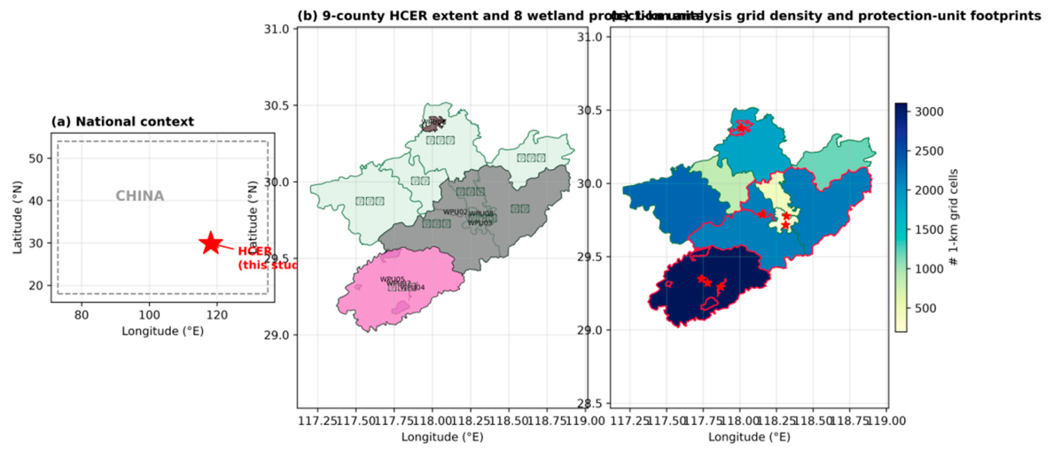
Figure 2.
Methodological workflow. Five sequential stages linking (i) 1-km grid and WPU polygon construction, (ii) four-dimensional CES modelling with Random Forest and XGBoost trained on 2010/2020 anchor labels, (iii) distance-decay exposure kernel construction, (iv) two-way fixed-effects panel regression with county-clustered SE, and (v) SHAP-based mechanism decomposition and three robustness checks.
Figure 2.
Methodological workflow. Five sequential stages linking (i) 1-km grid and WPU polygon construction, (ii) four-dimensional CES modelling with Random Forest and XGBoost trained on 2010/2020 anchor labels, (iii) distance-decay exposure kernel construction, (iv) two-way fixed-effects panel regression with county-clustered SE, and (v) SHAP-based mechanism decomposition and three robustness checks.
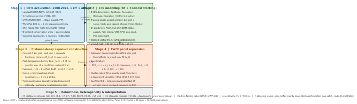
Figure 3.
Wetland surface water dynamics derived from MNDWI in the Huizhou Cultural-Ecological Reserve, 2000–2025. Panels (a)–(f): 5-year snapshots (2000, 2005, 2010, 2015, 2020, 2025) of surface-water pixels (blue) overlaid on the nine-county administrative boundary (thin black outlines) and the eight wetland protection units (red outlines). Land pixels shown in light grey. Inset bar chart: reserve-wide surface-water area (km²) by year. Data source: Landsat MOD09A1-derived MNDWI thresholded at zero, 30-m resolution resampled to 1-km grid.
Figure 3.
Wetland surface water dynamics derived from MNDWI in the Huizhou Cultural-Ecological Reserve, 2000–2025. Panels (a)–(f): 5-year snapshots (2000, 2005, 2010, 2015, 2020, 2025) of surface-water pixels (blue) overlaid on the nine-county administrative boundary (thin black outlines) and the eight wetland protection units (red outlines). Land pixels shown in light grey. Inset bar chart: reserve-wide surface-water area (km²) by year. Data source: Landsat MOD09A1-derived MNDWI thresholded at zero, 30-m resolution resampled to 1-km grid.
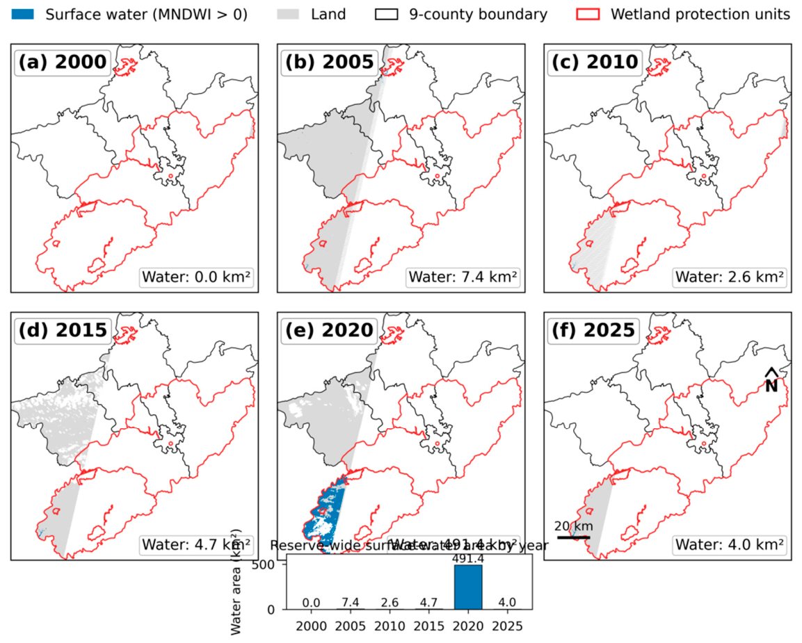
Figure 4.
Spatial pattern of four cultural ecosystem services (CES) dimensions across three time points, 2000/2010/2025. Rows: (top-to-bottom) CES1 Aesthetic, CES2 Recreation, CES3 Heritage, CES4 Education. Columns: (left-to-right) 2000, 2010, 2025. Values are XGBoost-predicted CES scores on the 1-km grid, normalized within each dimension by year-specific quantiles for cross-year comparability. Nine-county boundary in thin black outlines; eight wetland protection units in red outlines.
Figure 4.
Spatial pattern of four cultural ecosystem services (CES) dimensions across three time points, 2000/2010/2025. Rows: (top-to-bottom) CES1 Aesthetic, CES2 Recreation, CES3 Heritage, CES4 Education. Columns: (left-to-right) 2000, 2010, 2025. Values are XGBoost-predicted CES scores on the 1-km grid, normalized within each dimension by year-specific quantiles for cross-year comparability. Nine-county boundary in thin black outlines; eight wetland protection units in red outlines.
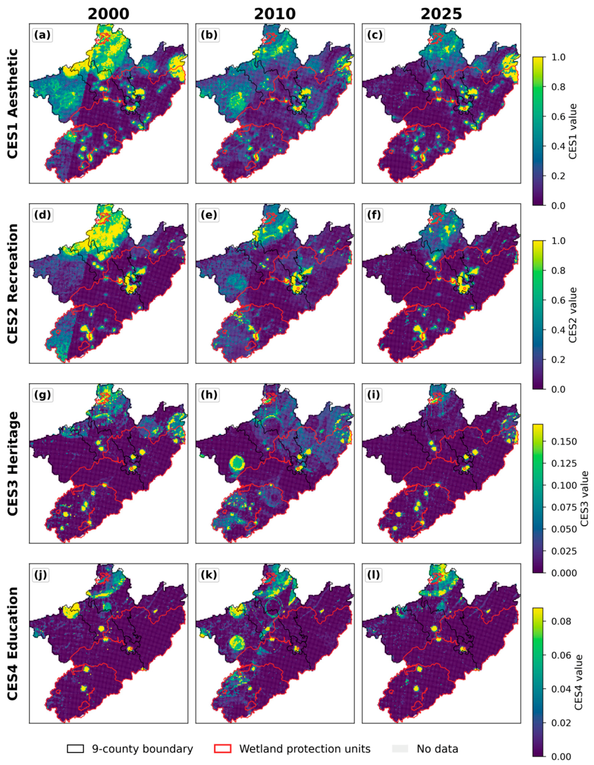
Figure 5.
SHAP predictor importance heat-map. Mean absolute SHAP value of each of the 14 predictors (X1–X14) for each of the four CES dimensions from the trained XGBoost regressors, computed over a stratified sample of 10 000 grid-year observations.
Figure 5.
SHAP predictor importance heat-map. Mean absolute SHAP value of each of the 14 predictors (X1–X14) for each of the four CES dimensions from the trained XGBoost regressors, computed over a stratified sample of 10 000 grid-year observations.
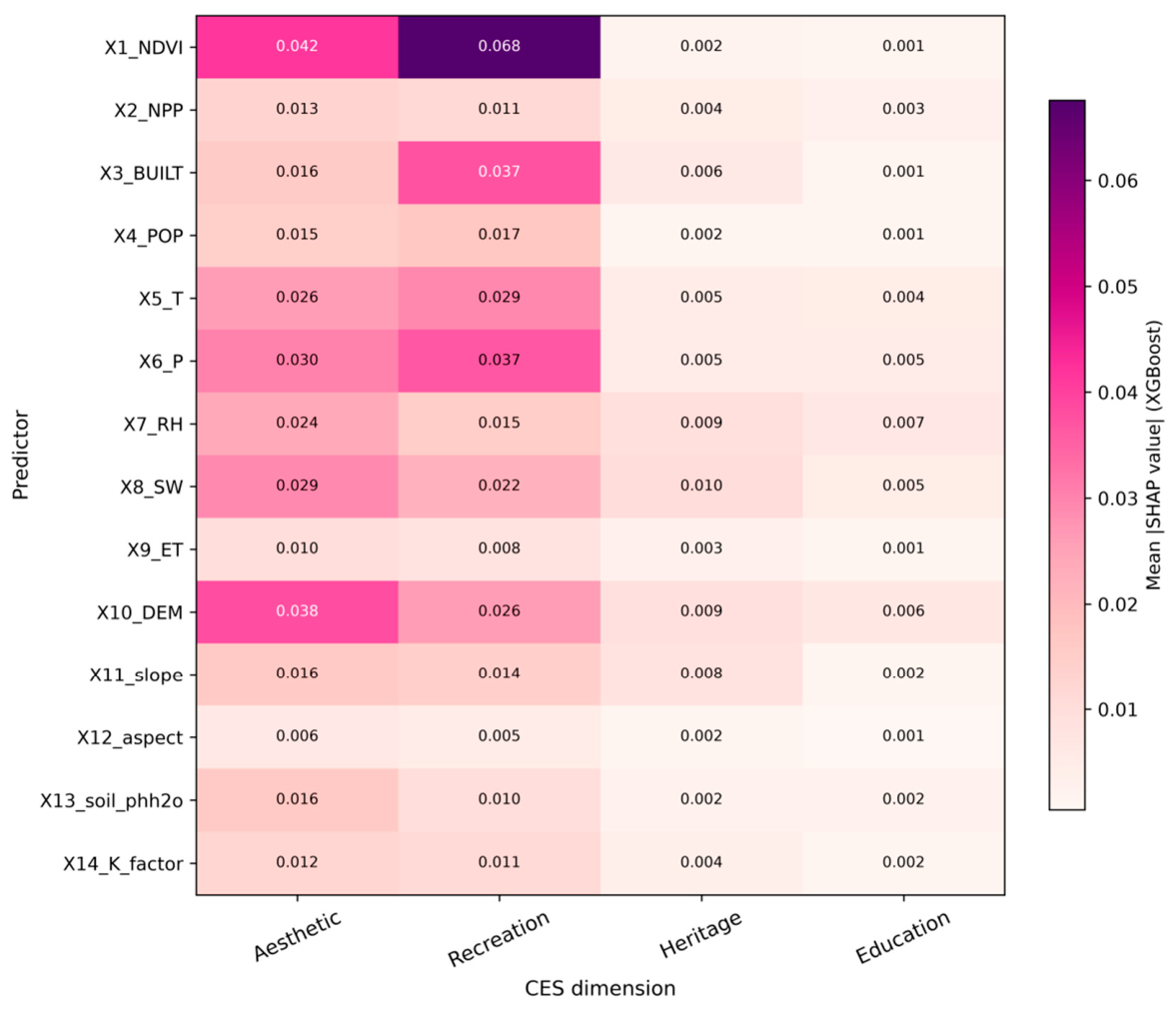
Figure 6.
Local indicators of spatial association (LISA) for CES-Total in 2000, 2010 and 2025. High-High (HH, deep red) and Low-Low (LL, deep blue) clusters indicate significant spatial concentration of high or low CES values; High-Low (HL, orange) and Low-High (LH, light blue) represent spatial outliers; non-significant grid cells (NS, light grey). LISA computed on n=14,011 1-km grids using k=8 nearest-neighbour weights with 999 permutations at α=0.05. Global Moran’s I values reported below each panel.
Figure 6.
Local indicators of spatial association (LISA) for CES-Total in 2000, 2010 and 2025. High-High (HH, deep red) and Low-Low (LL, deep blue) clusters indicate significant spatial concentration of high or low CES values; High-Low (HL, orange) and Low-High (LH, light blue) represent spatial outliers; non-significant grid cells (NS, light grey). LISA computed on n=14,011 1-km grids using k=8 nearest-neighbour weights with 999 permutations at α=0.05. Global Moran’s I values reported below each panel.
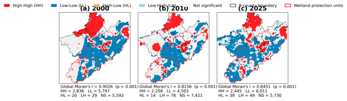
Figure 7.
Two-way fixed-effects main coefficients. Point estimates and 95 % confidence intervals of the exposure × post-designation coefficient β on the four CES dimensions and their composite CES-Total, with county-clustered standard errors and full M3 controls. λ = 5 km bandwidth.
Figure 7.
Two-way fixed-effects main coefficients. Point estimates and 95 % confidence intervals of the exposure × post-designation coefficient β on the four CES dimensions and their composite CES-Total, with county-clustered standard errors and full M3 controls. λ = 5 km bandwidth.
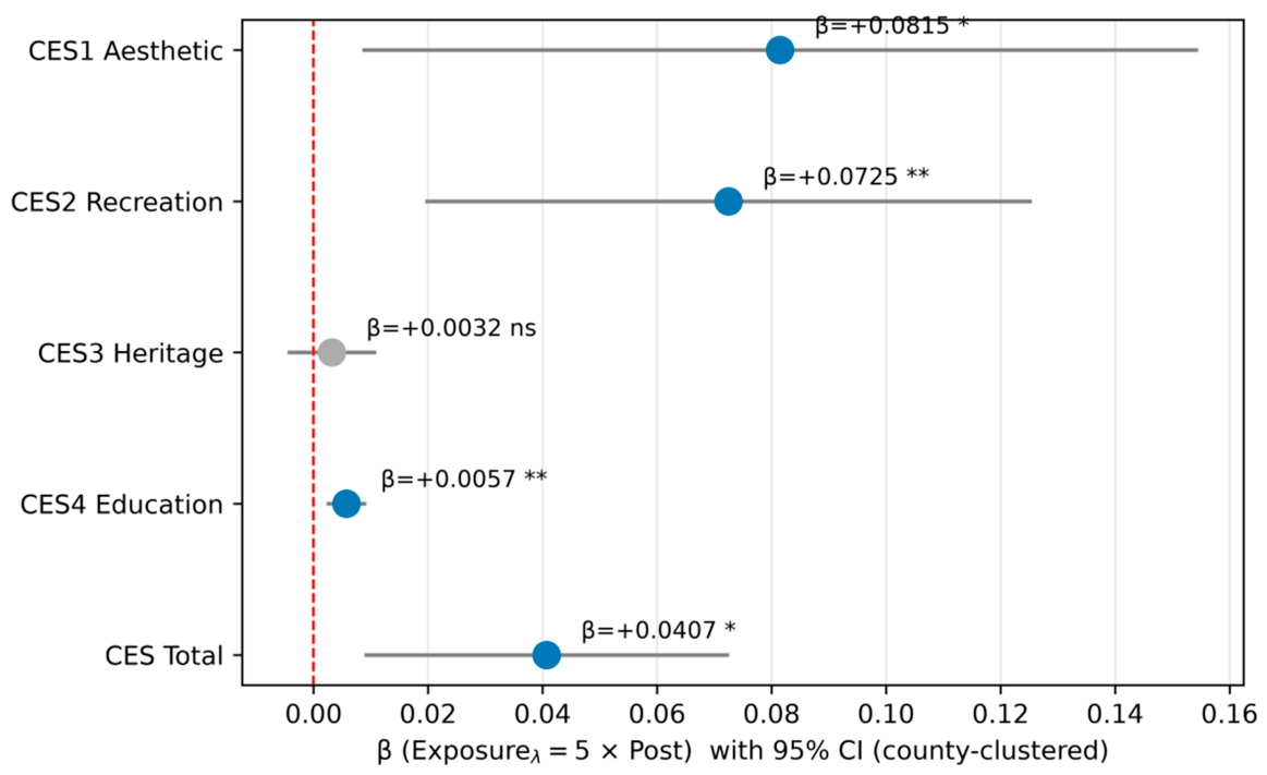
Figure 8.
Robustness and distance-response results. (a) Stepwise addition of controls (M0 → M3) for CES-Total, showing halving of the exposure coefficient once climate is controlled; (b) drop-Taiping-Lake sensitivity for the four CES dimensions and CES-Total; (c) decay-length λ sensitivity across λ ∈ {2, 5, 10} km; (d) distance-response halo of CES-Total across seven distance bins on the post-designation subsample.
Figure 8.
Robustness and distance-response results. (a) Stepwise addition of controls (M0 → M3) for CES-Total, showing halving of the exposure coefficient once climate is controlled; (b) drop-Taiping-Lake sensitivity for the four CES dimensions and CES-Total; (c) decay-length λ sensitivity across λ ∈ {2, 5, 10} km; (d) distance-response halo of CES-Total across seven distance bins on the post-designation subsample.
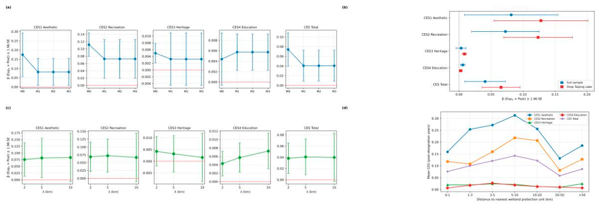
Figure 9.
Annual CES trajectories under v1 (anchor interpolation) versus v2 (fully annual real climate data) specifications for the four CES dimensions, 2000–2025. Grey lines with circular markers show the v1 series based on the anchor-interpolation covariate stack retained as the main specification; blue lines with square markers show the v2 series based on the fully annual NASA POWER + MODIS + WorldPop covariate stack. v2 trajectories exhibit substantial high-frequency inter-annual variability absent from the v1 series, driven by year-on-year climate and productivity fluctuations.
Figure 9.
Annual CES trajectories under v1 (anchor interpolation) versus v2 (fully annual real climate data) specifications for the four CES dimensions, 2000–2025. Grey lines with circular markers show the v1 series based on the anchor-interpolation covariate stack retained as the main specification; blue lines with square markers show the v2 series based on the fully annual NASA POWER + MODIS + WorldPop covariate stack. v2 trajectories exhibit substantial high-frequency inter-annual variability absent from the v1 series, driven by year-on-year climate and productivity fluctuations.
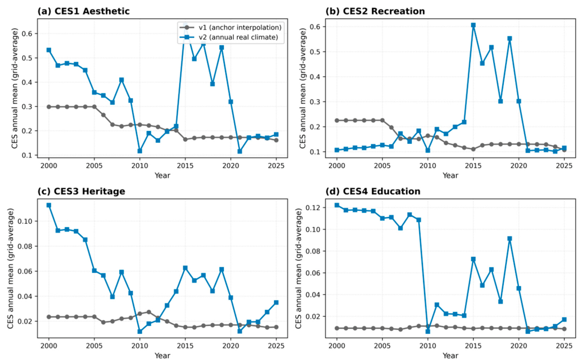
Figure 10.
Comparison of main β(Exp₅·Post) coefficients under v1 (anchor interpolation) and v2 (fully annual real climate) specifications, with 95 % confidence intervals. Grey circles denote v1 estimates; blue squares denote v2 estimates. The v2 exercise attenuates the amenity-anchored coefficients toward zero and reshuffles the CES4 Education coefficient sign, consistent with a measurement-error mechanism in which high-frequency climate noise dilutes the low-frequency exposure–Post interaction signal.
Figure 10.
Comparison of main β(Exp₅·Post) coefficients under v1 (anchor interpolation) and v2 (fully annual real climate) specifications, with 95 % confidence intervals. Grey circles denote v1 estimates; blue squares denote v2 estimates. The v2 exercise attenuates the amenity-anchored coefficients toward zero and reshuffles the CES4 Education coefficient sign, consistent with a measurement-error mechanism in which high-frequency climate noise dilutes the low-frequency exposure–Post interaction signal.
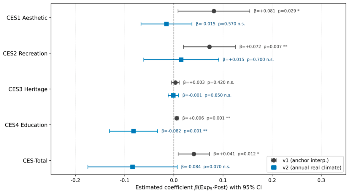

Table 1.
Data sources and preprocessing pipeline.
| # | Layer | Native resolution / period | Source | URL / DOI | Preprocessing |
| 1 | Landsat 5/7/8/9 surface reflectance (NDVI, EVI) | 30 m, 2000-2025 | USGS / GEE LANDSAT/LC08/C02/T1_L2 etc. | earthengine.google.com | Cloud-masked with CFmask, annual medoid composite, resampled to 1 km bilinear |
| 2 | MODIS LST (MOD11A2) | 1 km, 8-day, 2000-2025 | NASA LP-DAAC | lpdaac.usgs.gov | Annual mean of day/night LST |
| 3 | TerraClimate (Precip., VPD, SPEI) | ~4 km, monthly, 2000-2025 | Abatzoglou et al. [27] | climatologylab.org/terraclimate.html | Annual sum / mean, resampled to 1 km |
| 4 | SRTM v3 + ASTER GDEM (elevation, slope, aspect, TWI) | 30 m, static | USGS EarthExplorer | earthexplorer.usgs.gov | gdaldem slope / aspect / TWI; resampled to 1 km |
| 5 | WorldPop 100 m population | 100 m, annual 2000-2020 (extrapolated to 2025) | Tatem [28] | worldpop.org | Sum-aggregated to 1 km |
| 6 | OpenStreetMap roads / POI | Vector, 2010-2025 snapshots | OSM / Geofabrik | download.geofabrik.de | Kernel density estimation, resampled to 1 km |
| 7 | NPP-VIIRS night-time light | 500 m, monthly, 2012-2025 | NOAA/NGDC | eogdata.mines.edu | Annual median composite, resampled to 1 km |
| 8 | Wetland conservation unit polygons (8 units) | Vector | Anhui / Jiangxi Provincial Wetland Protection Announcements; Ramsar Info Sheet | forestry.gov.cn; ramsar.org | Standardised gazette-year field: multi-tier SOP (national first) |
| 9 | Huizhou Cultural-Ecological Reserve (HCER) boundary | Vector, est. 2008 | MoCTA gazette [15] | mct.gov.cn | Fixed, treated as background policy |
| 10 | Township & 9-county boundaries | Vector, 2020 | Resource and Environment Data Center, CAS | resdc.cn | Used for cluster-robust SE |
| 11 | Cultural heritage points (villages, halls, gazetteer sites) | Vector | China Cultural Relics Bureau; Huizhou District Gazetteer | ncha.gov.cn | Density kernel to 1 km |
| 12 | Geo-tagged social media photos (Flickr, Weibo, Mafengwo) | Point, 2010-2024 | API / public dumps | flickr.com/api; open.weibo.com | Deduplicated, kernel density; auxiliary CES label |
Table 2.
Cultural ecosystem service (CES) dimensions and their 1 km-annual remote-sensing / socio-spatial proxies.
Table 2.
Cultural ecosystem service (CES) dimensions and their 1 km-annual remote-sensing / socio-spatial proxies.
| Code | CES dimension | Working definition (CICES v5.1 subset) | Primary proxies (14 features stacked in RF + XGBoost) | Response unit |
| CES1 | Aesthetic | Perceived scenic quality of the landscape, including visual openness, greenness and topographic relief | NDVI, EVI, LST, slope, aspect, DEM relief, viewshed-corrected greenness, geo-tagged photo density | 1 km × annual |
| CES2 | Recreation | Opportunity for on-site leisure, sight-seeing, hiking and water-based recreation | POI density (scenic areas, home-stays, catering), road accessibility, night-time-light, distance to trails, water surface area | 1 km × annual |
| CES3 | Heritage | Presence and legibility of cultural heritage: Huizhou vernacular villages, ancestral halls, terraced tea and rice fields | Density of gazetteer-listed heritage points, historical village polygons, terrace-shaped GLCM texture on Landsat | 1 km × annual |
| CES4 | Education | Delivery of environmental / cultural education through nature-based classrooms, science parks and interpretation trails | Density of schools, museums, science bases, geo-referenced educational events, WorldPop-weighted access | 1 km × annual |
| — | CES_total | Standardised sum of CES1-CES4 (z-scored, then averaged) | Same 14 features; stacked meta-learner | 1 km × annual |
Notes: All four dimensions are trained with expert-scored labels blended with social-media geo-tagged photos (Flickr, Weibo, Mafengwo) using blocked spatial cross-validation [45]. Existence and Bequest values are conceptually acknowledged but omitted because no 1 km, 26-year remote-sensing proxy is credible for them (see Discussion 4.4).
Table 3.
Main TWFE panel results: effect of distance-decay wetland-conservation exposure on the four CES dimensions and their composite (λ = 5 km).
Table 3.
Main TWFE panel results: effect of distance-decay wetland-conservation exposure on the four CES dimensions and their composite (λ = 5 km).
| Dependent variable | β (Exp₅ · Post) | Cluster SE | t | p | 95 % CI | Sign |
| CES1 Aesthetic | +0.0815 | 0.0373 | 2.19 | 0.029 | [+0.008, +0.154] | + * |
| CES2 Recreation | +0.0724 | 0.0270 | 2.68 | 0.007 | [+0.020, +0.125] | + ** |
| CES3 Heritage | +0.0032 | 0.0040 | 0.81 | 0.420 | [-0.005, +0.011] | n.s. |
| CES4 Education | +0.0057 | 0.0018 | 3.24 | 0.001 | [+0.002, +0.009] | + *** |
| CES_total (composite) | +0.0407 | 0.0162 | 2.51 | 0.012 | [+0.009, +0.073] | + * |
Notes: Estimator: linearmodels.PanelOLS with grid fixed effects and year fixed effects. Cluster-robust standard errors at the county level (9 clusters). All models control for annual mean temperature (X5_T), annual precipitation (X6_P), relative humidity (X7_RH), built-up share (X3_BUILT) and population density (X4_POP); the static topographic controls (X10_DEM, X11_slope) are absorbed by grid FE. Sample: 14 011 grids × 26 years = 364 286 observations. Significance codes: * p<0.05, ** p<0.01, *** p<0.001.
Table 4.
Global Moran’s I of the four CES dimensions across three benchmark years (2000, 2010, 2025).
Table 4.
Global Moran’s I of the four CES dimensions across three benchmark years (2000, 2010, 2025).
| CES dimension | Year | n (grids) | Moran’s I | Expected I | z-score | p-value (999 perm.) | Interpretation |
| CES1 Aesthetic | 2000 | 14 011 | 0.8915 | −7.1 × 10⁻⁵ | 212.340 | 0.001 | Positive spatial autocorrelation |
| CES2 Recreation | 2000 | 14 011 | 0.9112 | −7.1 × 10⁻⁵ | 218.086 | 0.001 | Positive spatial autocorrelation |
| CES3 Heritage | 2000 | 14 011 | 0.7271 | −7.1 × 10⁻⁵ | 170.415 | 0.001 | Positive spatial autocorrelation |
| CES4 Education | 2000 | 14 011 | 0.7560 | −7.1 × 10⁻⁵ | 178.648 | 0.001 | Positive spatial autocorrelation |
| CES1 Aesthetic | 2010 | 14 011 | 0.7884 | −7.1 × 10⁻⁵ | 194.999 | 0.001 | Positive spatial autocorrelation |
| CES2 Recreation | 2010 | 14 011 | 0.8045 | −7.1 × 10⁻⁵ | 195.219 | 0.001 | Positive spatial autocorrelation |
| CES3 Heritage | 2010 | 14 011 | 0.7243 | −7.1 × 10⁻⁵ | 178.234 | 0.001 | Positive spatial autocorrelation |
| CES4 Education | 2010 | 14 011 | 0.7076 | −7.1 × 10⁻⁵ | 177.507 | 0.001 | Positive spatial autocorrelation |
| CES1 Aesthetic | 2025 | 14 011 | 0.8319 | −7.1 × 10⁻⁵ | 201.658 | 0.001 | Positive spatial autocorrelation |
| CES2 Recreation | 2025 | 14 011 | 0.8303 | −7.1 × 10⁻⁵ | 200.039 | 0.001 | Positive spatial autocorrelation |
| CES3 Heritage | 2025 | 14 011 | 0.7299 | −7.1 × 10⁻⁵ | 174.261 | 0.001 | Positive spatial autocorrelation |
| CES4 Education | 2025 | 14 011 | 0.7373 | −7.1 × 10⁻⁵ | 175.396 | 0.001 | Positive spatial autocorrelation |
Notes: XGBoost-inferred CES field values at 1-km grid resolution (n = 14 011 grids). Global Moran’s I is computed with a Queen-approximating k = 8 nearest-neighbour, row-standardised spatial weights matrix on grid centroids; the p-values are obtained by a 999-permutation reference distribution under the null of spatial randomness. All twelve I values are statistically significant at p = 0.001. The reported I magnitudes indicate strong positive spatial autocorrelation across all four CES dimensions and three benchmark years. This diagnostic is descriptive and does not enter the causal identification of §2.3.3 or §3.2.
Table 5.
Robustness and sensitivity results.
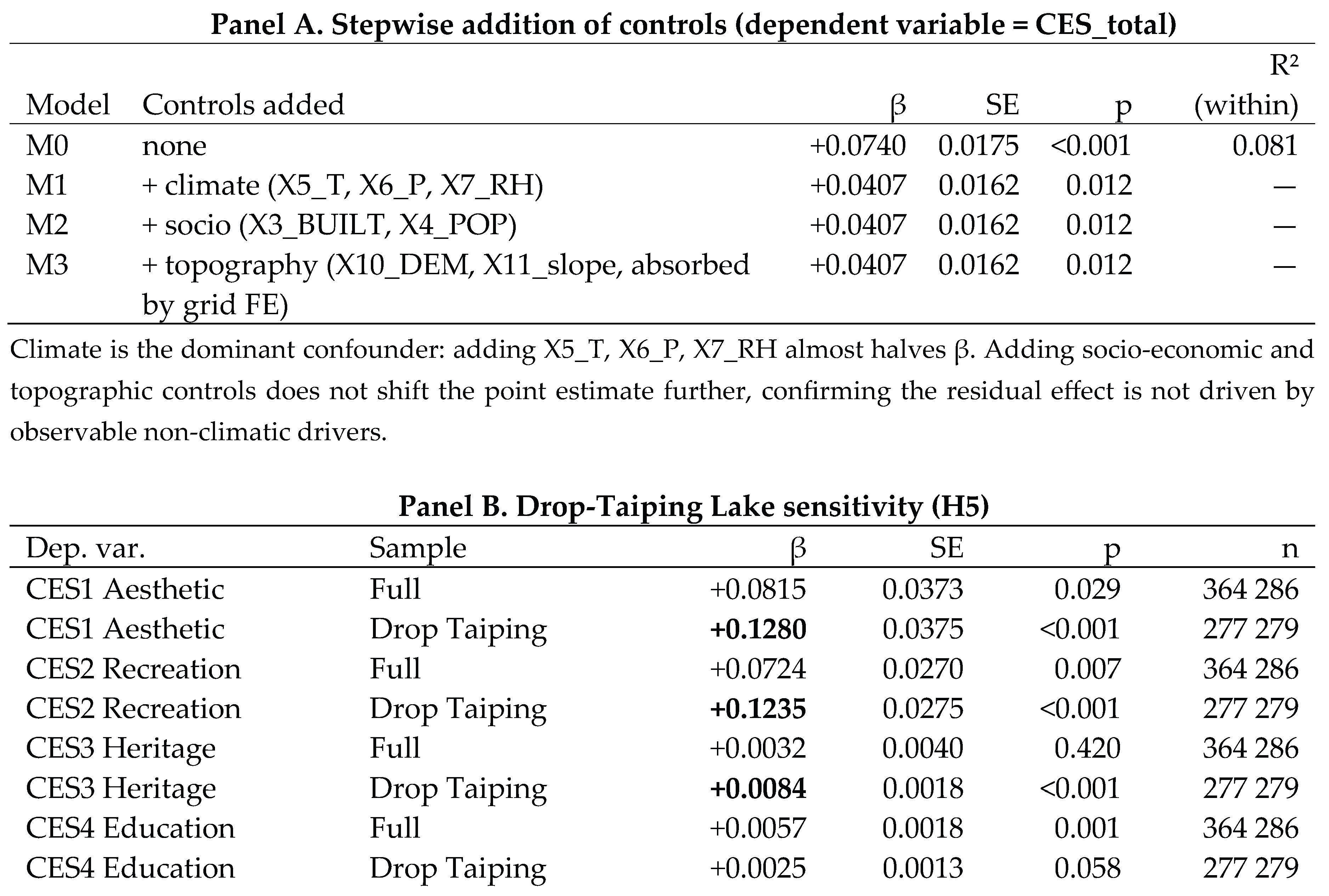
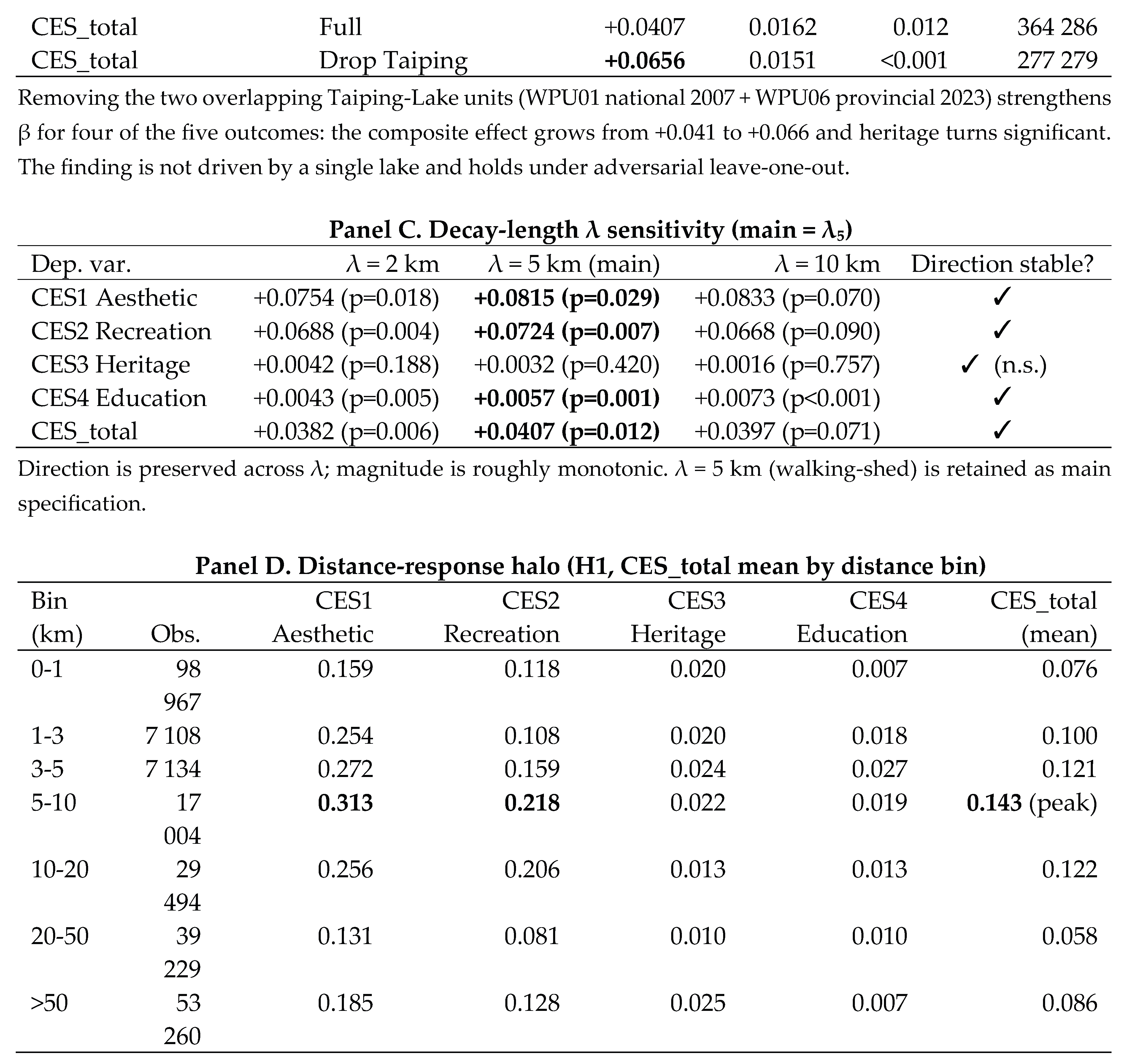
Table 6.
Sensitivity to climate data choice: main β(Exp₅·Post) coefficients under v1 (anchor interpolation) vs v2 (fully annual real climate data).
Table 6.
Sensitivity to climate data choice: main β(Exp₅·Post) coefficients under v1 (anchor interpolation) vs v2 (fully annual real climate data).
| Dependent variable | v1 β (main) | v1 p | v1 sig | v2 β | v2 p | v2 sig | Δβ (v2 − v1) |
| CES1 Aesthetic | +0.0815 | 0.029 | * | −0.015 | 0.57 | n.s. | −0.097 |
| CES2 Recreation | +0.0725 | 0.007 | ** | +0.015 | 0.70 | n.s. | −0.058 |
| CES3 Heritage | +0.0032 | 0.420 | n.s. | −0.001 | 0.85 | n.s. | −0.004 |
| CES4 Education | +0.0057 | 0.001 | *** | −0.082 | 0.001 | *** | −0.088 |
| CES-Total | +0.0407 | 0.012 | * | −0.084 | 0.07 | (*) | −0.125 |
Notes: v1 = main specification with anchor interpolation for X2–X9 covariates (Y1 = 2005, Y2 = 2015). v2 = sensitivity re-run with a fully annual real climate covariate stack (NASA POWER daily reanalysis aggregated to annual + MODIS MOD17A3HGF NPP + MODIS MOD16A3GF ET + WorldPop). Δβ = β(v2) − β(v1). Both specifications share the same eight wetland protection units, distance-decay exposure with λ = 5 km, county-clustered standard errors and 364 286 grid-year observations from a two-way fixed-effects panel regression. Significance codes: * p < 0.05, ** p < 0.01, *** p < 0.001, (*) p < 0.10.
Disclaimer/Publisher’s Note: The statements, opinions and data contained in all publications are solely those of the individual author(s) and contributor(s) and not of MDPI and/or the editor(s). MDPI and/or the editor(s) disclaim responsibility for any injury to people or property resulting from any ideas, methods, instructions or products referred to in the content. |
© 2026 by the authors. Licensee MDPI, Basel, Switzerland. This article is an open access article distributed under the terms and conditions of the Creative Commons Attribution (CC BY) license (http://creativecommons.org/licenses/by/4.0/).
Copyright: This open access article is published under a Creative Commons CC BY 4.0 license, which permit the free download, distribution, and reuse, provided that the author and preprint are cited in any reuse.


