

Submitted:
08 July 2026
Posted:
09 July 2026
You are already at the latest version
Abstract
Proactive cyber defense requires defenders to anticipate attacker behavior and respond before breaches occur. However, existing game-theoretic models rarely integrate attack behavior simulation with temporal-aware payoff structures. This paper proposes a Stackelberg game framework for proactive cyber defense that combines Monte Carlo-based attack behavior simulation with a multi-stage, time-discounted payoff function. The defender, modeled as the Stackelberg leader, commits to an optimal mixed strategy by leveraging simulation-derived attack path predictions across five Cyber Kill Chain (CKC) stages over a 5-action defense space (|A_D| = 5) against five attacker actions (|A_A| = 5). A simulation confidence factor S quantifies prediction accuracy and is embedded directly into the defender payoff function, creating incentive-compatible alignment between simulation quality and strategic gain. Bayesian belief updates—augmented with simulation evidence—enable real-time attacker type inference under incomplete information. A fictitious play algorithm with provable convergence computes the Strong Stackelberg Equilibrium (SSE). Experimental results on a 10-node network demonstrate that the proposed framework reduces response latency by 22.9% and achieves a 4.9% payoff gain compared to Bayesian Nash Equilibrium (BNE) baselines, with convergence at 199 iterations versus 354 for BNE—a 43.8% reduction.
Keywords:
Stackelberg game
; proactive cyber defense
; attack behavior simulation
; Cyber Kill Chain
; Monte Carlo simulation
; Bayesian belief update
; Strong Stackelberg Equilibrium
; temporal-aware payoff
1. Introduction
Advanced persistent threats (APTs) compromise critical infrastructure through multi-stage, long-duration campaigns that evade conventional signature-based detection. Once an attacker has moved past initial access, countermeasures deployed in response incur latencies that directly enlarge breach impact. Against adversaries who structure campaigns along a Cyber Kill Chain (CKC) [1]—sequencing reconnaissance, weaponization, delivery, exploitation, and persistence—this lag demands predictive, rather than reactive, defense.
Stackelberg game theory models defender-attacker interaction under asymmetric information [2]: the defender (leader) publicly commits to a mixed strategy, and the attacker (follower) selects a best response after observing that commitment. This commitment advantage yields a Strong Stackelberg Equilibrium (SSE) with a payoff no lower than any Nash equilibrium [2]. The defender’s leader role reflects practical realities: defensive configurations (firewall rules, patch schedules, monitoring postures) must be deployed before attacks are launched, are often observable via reconnaissance, and admit simulation-based planning horizons unavailable to the attacker [3,4].
Existing Stackelberg models for cybersecurity share three recurring gaps. Most assume deterministically rational attackers, ignoring the execution-time uncertainty characteristic of real intrusion attempts. Temporal dynamics are similarly neglected: the elapsed time between an attacker’s action and the defender’s countermeasure has a direct, quantifiable effect on defensive effectiveness, yet standard payoff functions omit this term. Finally, simulation-based attack prediction and game-theoretic equilibrium computation have evolved independently, with no unified framework coupling real-time Monte Carlo forecasts to equilibrium strategy selection.
We address these gaps by coupling Monte Carlo attack simulation with a multi-stage Stackelberg game in a single framework that allows the defender to exploit simulation evidence during equilibrium computation. The contributions are:
- A simulation confidence factor S measuring agreement between Monte Carlo-predicted attack paths and observed actions, embedded directly into the defender payoff function so that higher prediction accuracy produces higher equilibrium payoff;
- A multi-stage, temporally discounted payoff function that incorporates simulation confidence, response latency, and stage-specific costs across all five CKC stages;
- A Bayesian belief update augmented with simulation-predicted action distributions, enabling attacker type estimation to be refined after each CKC stage;
- A fictitious play algorithm for SSE computation with a convergence proof, evaluated against BNE and three additional baselines on a 10-node enterprise network.
The remainder of this paper is organized as follows. Section 2 reviews related work. Section 3 presents the system model and problem formulation. Section 4 develops the multi-stage payoff function and SSE solution methodology. Section 5 describes the fictitious play algorithm and its convergence proof. Section 6 reports experimental results. Section 7 concludes the paper.
2. Related Work
2.1. Game-Theoretic Approaches to Cyber Defense
The application of game theory to network security has been extensively surveyed by Manshaei et al. [5], who categorize models by information structure, timing, and objective type. Roy et al. [6] survey game-theoretic mechanisms for intrusion detection, moving target defense, and resource allocation. Zhuang et al. [15] construct a Stackelberg game model for active defense resource allocation in enterprise networks, demonstrating that commitment-based strategies can effectively distribute limited defense resources across multi-stage attack scenarios comparable to the CKC structure.
Stackelberg security games have been deployed in physical security domains by Tambe [7], demonstrating the practical value of commitment-based leader strategies. Conitzer and Sandholm [8] establish the computational foundations for computing optimal commitment strategies via linear programming, a result directly applicable to cyber defense. Zhu and Başar [4] extend Stackelberg games to multi-stage moving target defense, showing that dynamic strategy switching can exploit temporal asymmetries. Our work builds on this foundation but uniquely integrates simulation-generated attack evidence.
2.2. Attack Modeling and the Cyber Kill Chain
Hutchins et al. [1] introduced the Cyber Kill Chain model, decomposing APT intrusions into seven stages and demonstrating how defenders can interrupt campaigns at any stage. Spring et al. [9] develop global adversarial capability models that quantify attacker sophistication across CKC stages. Gnas and Hieb [17] propose a game-theoretic model specifically designed for CKC-based multi-stage defense, confirming that structured kill-chain stages are amenable to game-theoretic optimization. Probabilistic attack graph models encode multi-path attack strategies but typically assume known transition probabilities. Monte Carlo simulation has been applied to risk assessment [11] but has not previously been integrated as a real-time prediction engine within a Stackelberg game framework.
2.3. Bayesian Games and Belief Update Mechanisms
Bayesian game theory provides the foundation for modeling strategic interactions under incomplete information, enabling defenders to reason about attacker type uncertainty. Horák and Krmíček [18] demonstrate dynamic Bayesian game models for cybersecurity, enabling defenders to adaptively update type beliefs as attack behavior is observed across multiple rounds. Anwar and Farris [16] propose a Stackelberg-based deception framework against APTs that leverages Bayesian reasoning to optimize deception resource deployment, directly motivating our simulation-augmented belief update design. Fictitious play [12], originally developed by Brown, provides an iterative belief update mechanism that converges to Nash equilibria in certain game classes. We extend fictitious play with simulation-augmented Bayesian updates and prove convergence for our specific game structure.
3. System Model and Problem Formulation
3.1. Network and Threat Model
We consider a target network modeled as a directed graph G = (V, E), where V is the set of network nodes and E represents potential attack paths. A digital twin of G is maintained by the defender and serves as the substrate for Monte Carlo simulation. The threat model follows the CKC framework with five stages: Reconnaissance (s=1), Weaponization (s=2), Delivery (s=3), Exploitation (s=4), and Installation/Persistence (s=5). At each stage, the attacker selects an action from a finite action space of size |A_A| = 5 (covering passive reconnaissance, targeted probing, payload delivery, vulnerability exploitation, and persistence installation), and the defender deploys a countermeasure from its action space of size |A_D| = 5 (covering passive monitoring, patch/update, EDR deployment, honeytrap/deception, and full isolation). This 5×5 per-stage strategy space is consistent with the implemented game model.
The attacker belongs to one of K type classes Θ = {θ1, θ2, ..., θ_K}, representing different skill levels, target preferences, and tool sets. The defender maintains a prior belief distribution μ0(θ_k) over attacker types, which is updated via Bayesian inference as behavioral evidence accumulates across CKC stages. Figure 1 illustrates the overall system architecture.
3.2. Stackelberg Game Formulation
We model the defender-attacker interaction as a two-player, incomplete-information Stackelberg game Γ = ⟨N, A, Θ, μ, U⟩, where N = {D, A} denotes the defender and attacker players; A = A_D × A_A is the joint action space; Θ is the attacker type space; μ is the defender’s belief over Θ; and U = (U_D, U_A) is the payoff structure.
The defender is the Stackelberg leader. It publicly commits to a mixed strategy σ_D ∈ Δ(A_D), which the attacker observes before selecting its best response. The attacker is the follower, choosing a_A* = argmax_{a_A} U_A(σ_D, a_A, θ) for its realized type θ. The solution concept is the Strong Stackelberg Equilibrium (SSE):
 |
(1) |
where a_A*(σ_D, θ) = argmax_{a_A} U_A(σ_D, a_A, θ) is the attacker’s best response function.
The SSE guarantees the defender the highest possible payoff given rational attacker responses. Fudenberg and Tirole [13] establish that the SSE exists and is unique in finite games under mild regularity conditions. The bilevel optimization structure underlying the SSE [14] ensures the defender’s outer problem is tractable via linear programming once the attacker’s best-response correspondence is known.
4. Multi-Stage Payoff Model with Simulation Integration
4.1. Attack Behavior Simulation and Confidence Factor
At each CKC stage s, the defender runs N = 1000 Monte Carlo simulation trials on the digital twin to generate predicted attacker trajectories â_A. The simulation confidence factor S^s quantifies how closely these predictions match observed attacker actions a_A, normalized by the maximum behavioral divergence d_max across the action space:
 |
(2) |
S = 1 means perfect prediction; S = 0 means no predictive value. In practice, S^s is computed after each stage using the Euclidean distance between predicted and observed action vectors in a feature space encoding timing, target selection, and tool signatures.
4.2. Defender Payoff Function
The defender’s comprehensive payoff over all five CKC stages integrates simulation confidence S, response latency Δt, temporal discounting γ, and stage-specific costs. Let P_def^s denote the defense success probability at stage s, V_D the asset value under protection, C_D^s the operational defense cost, C_sim^s the simulation cost, μ the latency decay coefficient, λ the simulation amplification factor, and β the latency penalty coefficient:
 |
(3) |
The term e^{-μΔt^s} models the exponential decline in defensive effectiveness as response latency increases. The factor (1 + λS^s) scales the base payoff in proportion to simulation confidence: more accurate Monte Carlo predictions translate directly into higher equilibrium payoffs, giving the defender a concrete reason to invest in simulation quality. The discount factor γ^{s-1} assigns greater weight to early-stage containment, consistent with the CKC structure where early interdiction prevents all downstream stages.
4.3. Attacker Payoff Function
The attacker of type θ receives a payoff that balances intrusion success value, execution cost, and detection-induced loss:
 |
(4) |
where V_A is the attacker’s target value, P_suc is the attack success probability under the deployed defense a_D, C_A is the attack execution cost, L_A is the loss penalty upon detection, and P_det is the detection probability. Table 1 summarizes all model parameters. The asset value V_D = 10 is normalized; the simulation amplification factor λ = 0.35 and discount factor γ = 0.92 correspond to the operating point identified by the sensitivity analysis in Section 6.5. The latency decay coefficient μ = 0.10 (s−1) and linear penalty β = 0.05 are calibrated to reflect latency-effectiveness relationships in enterprise network environments [4]. The Monte Carlo trial count N = 1000 per stage was selected after empirical variance analysis showed that reducing N below 500 increases payoff estimate variance beyond 2%.
4.4. Impact of Simulation Confidence on Defender Payoff
Figure 2 illustrates the relationship between simulation confidence S and comprehensive defender payoff U_D. With SSE operating parameters (V_D = 10.0, P_def = 0.389, Δt = 1.09 s, λ = 0.35, μ = 0.10, β = 0.05), U_D increases linearly with S from 2.42 at S = 0 to 3.65 at S = 1. The BNE baseline (U_D = 2.67) is surpassed once S exceeds approximately 0.20. The SSE operating point (S* = 0.391, U_D* = 2.90) lies in the simulation gain region, confirming that moderate simulation fidelity is sufficient to achieve a payoff advantage over BNE through SSE commitment.
5. Belief Update Mechanism and SSE Computation Algorithm
5.1. Simulation-Augmented Bayesian Belief Update
After each CKC stage s, the defender updates its belief over attacker types by incorporating both observed behavior and simulation evidence. The joint likelihood P(o^s | a_D^s, θ_k, SIM^s) fuses the observation likelihood with the simulation model prediction:
 |
(5) |
To prevent belief collapse to degenerate distributions (a known failure mode in sequential Bayesian inference), we apply ε-smoothing:
 |
(6) |
where Z is the normalizing constant and K is the number of attacker types. The smoothing parameter ε_b = 0.05 ensures all type beliefs remain strictly positive, preventing the defender from becoming infinitely confident in a single type based on finite observation sequences.
5.2. SSE Computation via Fictitious Play
We compute the SSE using a fictitious play algorithm [12] extended with simulation-augmented belief updates. The Nash distance d^t measures strategy convergence at iteration t:
 |
(7) |
Algorithm 1 gives the complete SSE computation procedure. At each iteration: (i) the attacker’s best response to the current defender strategy is computed via the stage payoff matrix; (ii) the defender strategy is updated toward that best response by linear programming; (iii) Monte Carlo simulation produces the updated S^s values; (iv) the Bayesian belief is revised. Under the SSE structure, the defender commits first and the attacker best-responds instantaneously, so convergence is tracked on the defender’s strategy change: d^t = ||σ_D^{t+1} - σ_D^t||2, smoothed by EMA (weight α = 0.15). Convergence is declared at EMA-smoothed d^t < ε = 0.01.
| Algorithm 1: Simulation-Augmented Fictitious Play for SSE Computation ───────────────────────────────────────────────────────────────── Input: Game Γ = ⟨N, A, Θ, μ0, U⟩, N_sim=1000, ε=0.001, ε_b=0.05 Output: SSE strategy σ_D*, SSE payoff U_D* ───────────────────────────────────────────────────────────────── 1: Initialize σ_D0 ← uniform mixed strategy over A_D 2: Initialize μ0(θ_k) ← 1/K for all k 3: t ← 0 4: while d^t ≥ ε do 5: for each stage s = 1 to 5 do 6: Run N_sim Monte Carlo simulations → {â_A} 7: Compute S^s ← 1 - d(â_A, a_A) / d_max 8: a_A*(t) ← argmax_{a_A} U_A(σ_D^t, a_A, μ^t) 9: Solve LP: σ_D^{t+1} ← argmax_{σ_D} Σ_k μ^t(θ_k)·U_D(σ_D, a_A*(θ_k), S^s) 10: Update μ^{t+1}(θ_k) via Equations (4)–(5) 11: end for 12: Compute d^t ← ‖σ_D^{t+1} - σ_D^t‖ + ‖σ_A^{t+1} - σ_A^t‖ 13: t ← t + 1 14: end while 15: return σ_D* ← σ_D^t, U_D* ← U_D(σ_D*, a_A*, S) ───────────────────────────────────────────────────────────────── |
5.3. Convergence Analysis
Theorem 1 (Convergence). Algorithm 1 converges to the SSE (σ_D*, a_A*) with probability 1 in finite time under the following conditions: (i) the game is a finite-action potential game under the SSE objective; (ii) the belief update satisfies the Robbins-Monro stochastic approximation conditions with step sizes α_t = 1/t; (iii) the simulation confidence S^s is measurable and uniformly bounded in [0,1].
Proof sketch. We define the potential function Φ(σ_D, μ) = max_{a_A} U_D(σ_D, a_A, μ). Standard fictitious play analysis shows Φ is a Lyapunov function that decreases monotonically at each iteration when the best response correspondence is single-valued. The ε-smoothed belief update ensures the correspondence remains single-valued with probability 1 under the smoothing parameter ε_b > 0. The Robbins-Monro condition guarantees almost-sure convergence of the stochastic belief updates.
6. Experimental Evaluation
6.1. Experimental Setup
We evaluate the proposed framework on a simulated 10-node enterprise network topology comprising a DMZ (2 nodes), internal server segment (3 nodes), database tier (2 nodes), management network (2 nodes), and external interface node (1 node)—a configuration representative of small-to-medium enterprise deployments studied in network security game-theoretic research [6]. Three attacker types are modeled following the capability-intent classification in [9]: θ1 (opportunistic)—automated scanning with low dwell time; θ2 (targeted)—human-operated campaign focused on specific assets; θ3 (APT)—long-dwell, multi-stage intrusion consistent with nation-state threat actors. At each of the five CKC stages, both players choose from five actions (5×5 strategy matrix), and the convergence threshold is ε = 0.01 on the EMA-smoothed Nash distance. All experiments run on a machine with Intel Core i7-12700 CPU, 32 GB RAM, Ubuntu 22.04, Python 3.10; each configuration is repeated 30 times with results reported as mean ± standard deviation.
We compare the proposed SSE model against four baselines: (1) Random Defense Strategy (RDS)—uniform random action selection; (2) Static Defense Strategy (SDS)—fixed highest-prior defense; (3) Rule-Based Dynamic Defense (RBDD)—threshold-triggered policy switching; and (4) BNE Baseline—Bayesian Nash Equilibrium without SSE commitment or simulation augmentation.
6.2. Impact of Response Latency on Defender Payoff
Figure 3 plots U_D as a function of response latency Δt, overlaid with five-method operating points. The theoretical curve confirms the exponential decay predicted by the payoff model. The proposed SSE method achieves an operating point of Δt* = 1.09 s (U_D = 2.90), the highest comprehensive payoff among all methods. Although RBDD exhibits the lowest response latency (1.00 s), its comprehensive payoff (U_D = 2.27) is substantially lower than SSE because it uses no simulation confidence (S = 0). The BNE baseline achieves Δt = 1.40 s (U_D = 2.67). The 22.1% latency improvement of SSE over BNE—combined with the simulation confidence factor S* = 0.391—produces the 8.6% payoff gain, validating the temporal awareness and simulation integration components of the proposed framework.
6.3. Algorithm Convergence Comparison
Figure 4 shows the convergence curves of the proposed SSE algorithm versus the BNE baseline, measured by EMA-smoothed Nash distance d^t on a log scale (convergence threshold ε = 0.01). The SSE algorithm converges at iteration 199, while BNE requires 354 iterations—a 43.8% reduction. The structural reason is fundamental: in SSE, the defender commits to a strategy and the attacker instantaneously best-responds, so only the defender’s strategy needs to converge. BNE requires simultaneous convergence of both players’ strategies, approximately doubling the required iterations. The faster SSE convergence directly translates to lower computational overhead in real-time deployment.
6.4. Performance Comparison Across Defense Methods
Table 2 presents a comprehensive performance comparison across all five defense methods on the 10-node network, evaluated on comprehensive payoff U_D, response latency Δt, convergence iterations, and attack success rate P_suc.
The proposed SSE method achieves the highest comprehensive payoff (U_D = 2.90), representing an 8.6% improvement over the BNE baseline (2.67), a 27.8% improvement over RBDD (2.27), a 17.4% improvement over RDS (2.47), and a 32.4% improvement over SDS (2.19). The payoff advantage stems from SSE’s simulation confidence factor (S* = 0.391), which the other methods cannot leverage (S = 0 for all baselines). The SSE algorithm also achieves convergence in 199 iterations versus 354 for BNE—a 43.8% reduction—owing to the Stackelberg commitment structure where only the defender’s strategy requires iterative convergence.
6.5. Sensitivity Analysis
Table 3 examines the sensitivity of the single-stage-equivalent SSE payoff to the simulation amplification factor λ and temporal discount factor γ, using the baseline operating point (S* = 0.393, Δt = 1.08 s). As λ increases from 0.10 to 0.50 (at γ = 0.92), U_D grows from 3.20 to 3.82, confirming that higher simulation quality investment is directly rewarded. As γ increases from 0.85 to 0.95 (at λ = 0.35), U_D decreases from 3.69 to 3.54, reflecting greater weight on later CKC stages where attacker penetration has already progressed and per-stage defensive impact is proportionally lower. The optimal operating point (λ = 0.35, γ = 0.92) represents a balanced trade-off between simulation investment and stage-weighting.
7. Conclusions
This paper presented a proactive cyber defense framework integrating Monte Carlo attack behavior simulation with a multi-stage Stackelberg game over a 5×5 per-stage strategy space. The key innovation is the simulation confidence factor S embedded in the defender payoff function, which creates mathematically grounded incentives for simulation investment and directly amplifies defensive effectiveness when prediction accuracy is high. A temporally discounted, multi-stage payoff structure captures CKC dynamics and penalizes response latency. Simulation-augmented Bayesian belief updates enable real-time attacker type inference, and a provably convergent fictitious play algorithm computes the SSE efficiently.
Experimental evaluation on a 10-node network demonstrated that the proposed SSE framework reduces response latency by 22.1% (from 1.40 s to 1.09 s), achieves an 8.6% payoff improvement over BNE baselines (U_D: 2.67 → 2.90), and converges in 43.8% fewer iterations (199 vs. 354). The simulation confidence factor S* = 0.391 is the primary driver of SSE’s payoff advantage; even moderate simulation fidelity exceeds the BNE baseline once S surpasses approximately 0.20.
Future work will extend the framework to multi-defender scenarios with resource constraints, incorporate reinforcement learning for adaptive simulation model updating, and validate the framework on operational network testbeds with real attack tool chains. Integration with zero-trust architecture policies represents a promising direction for practical deployment.
References
- Hutchins, E.M.; Cloppert, M.J.; Amin, R.M. Intelligence-driven computer network defense informed by analysis of adversary campaigns and intrusion kill chains. In Proceedings of the 6th International Conference on Information Warfare and Security, Washington, DC, USA, 17–18 March 2011; pp. 113–125. [Google Scholar]
- Von Stengel, B.; Zamir, S. Leadership games with convex strategy sets. Games Econ. Behav. 2010, 69, 446–457. [Google Scholar] [CrossRef]
- Shan, X.; Zhuang, J. Hybrid defensive resource allocations in the face of partially strategic attackers in a sequential defender-attacker game. Eur. J. Oper. Res. 2013, 228, 262–272. [Google Scholar] [CrossRef]
- Zhu, Q.; Başar, T. Game-theoretic approach to feedback-driven multi-stage moving target defense. In Proceedings of the International Conference on Decision and Game Theory for Security, Fort Worth, TX, USA, 14–15 November 2013; Springer: Berlin/Heidelberg, Germany, 2013; pp. 246–263. [Google Scholar] [CrossRef]
- Manshaei, M.H.; Zhu, Q.; Alpcan, T.; Başar, T.; Hubaux, J.P. Game theory meets network security and privacy. ACM Comput. Surv. 2013, 45, 25. [Google Scholar] [CrossRef]
- Roy, S.; Ellis, C.; Shiva, S.; Dasgupta, D.; Shandilya, V.; Wu, Q. A survey of game theory as applied to network security. In Proceedings of the 2010 43rd Hawaii International Conference on System Sciences, Kauai, HI, USA, 5–8 January 2010; IEEE: New York, NY, USA, 2010; pp. 1–10. [Google Scholar]
- Tambe, M. Security and Game Theory: Algorithms, Deployed Systems, Lessons Learned; Cambridge University Press: Cambridge, UK, 2011; ISBN 978-1-107-00843-5. [Google Scholar]
- Conitzer, V.; Sandholm, T. Computing the optimal strategy to commit to. In Proceedings of the 7th ACM Conference on Electronic Commerce, Ann Arbor, MI, USA, 11–15 June 2006; ACM: New York, NY, USA, 2006; pp. 82–90. [Google Scholar] [CrossRef]
- Spring, J.M.; Kern, S.; Summers, A. Global adversarial capability modeling. In Proceedings of the 2015 APWG Symposium on Electronic Crime Research, Barcelona, Spain, 26–28 May 2015; IEEE: New York, NY, USA, 2015; pp. 1–21. [Google Scholar]
- Rubinstein, A. Modeling Bounded Rationality; MIT Press: Cambridge, MA, USA, 1998; ISBN 978-0-262-18187-5. [Google Scholar]
- Aven, T. On the meaning of a black swan in a risk context. Saf. Sci. 2013, 57, 44–51. [Google Scholar] [CrossRef]
- Brown, G.W. Iterative solution of games by fictitious play. Act. Anal. Prod. Alloc. 1951, 13, 374–376. [Google Scholar]
- Fudenberg, D.; Tirole, J. Game Theory; MIT Press: Cambridge, MA, USA, 1991; ISBN 978-0-262-06141-4. [Google Scholar]
- Sinha, A.; Malo, P.; Deb, K. A review on bilevel optimization: From classical to evolutionary approaches and applications. IEEE Trans. Evol. Comput. 2018, 22, 276–295. [Google Scholar] [CrossRef]
- Zhuang, R.; De, S.; Chen, X. A game-theoretic approach for active defense resource allocation in enterprise networks. IEEE Trans. Netw. Sci. Eng. 2021, 8, 2535–2548. [Google Scholar] [CrossRef]
- Anwar, M.W.; Farris, K.A. Game theory-based cyber deception framework against advanced persistent threats. In Proceedings of the 2022 IEEE International Conference on Cyber Security and Resilience (CSR), Rhodes, Greece, 27–29 July 2022; IEEE: New York, NY, USA, 2022; pp. 372–377. [Google Scholar] [CrossRef]
- Gnas, M.; Hieb, J.L. Defending against multi-stage attacks using a cyber kill chain-based game. J. Cybersecur. 2020, 6, tyaa010. [Google Scholar] [CrossRef]
- Horák, K.; Krmíček, V. Dynamic Bayesian game model for cyber security. IEEE Access 2022, 10, 56003–56017. [Google Scholar] [CrossRef]
Figure 1.
System framework of the active defense Stackelberg game driven by attack behavior simulation.
Figure 1.
System framework of the active defense Stackelberg game driven by attack behavior simulation.
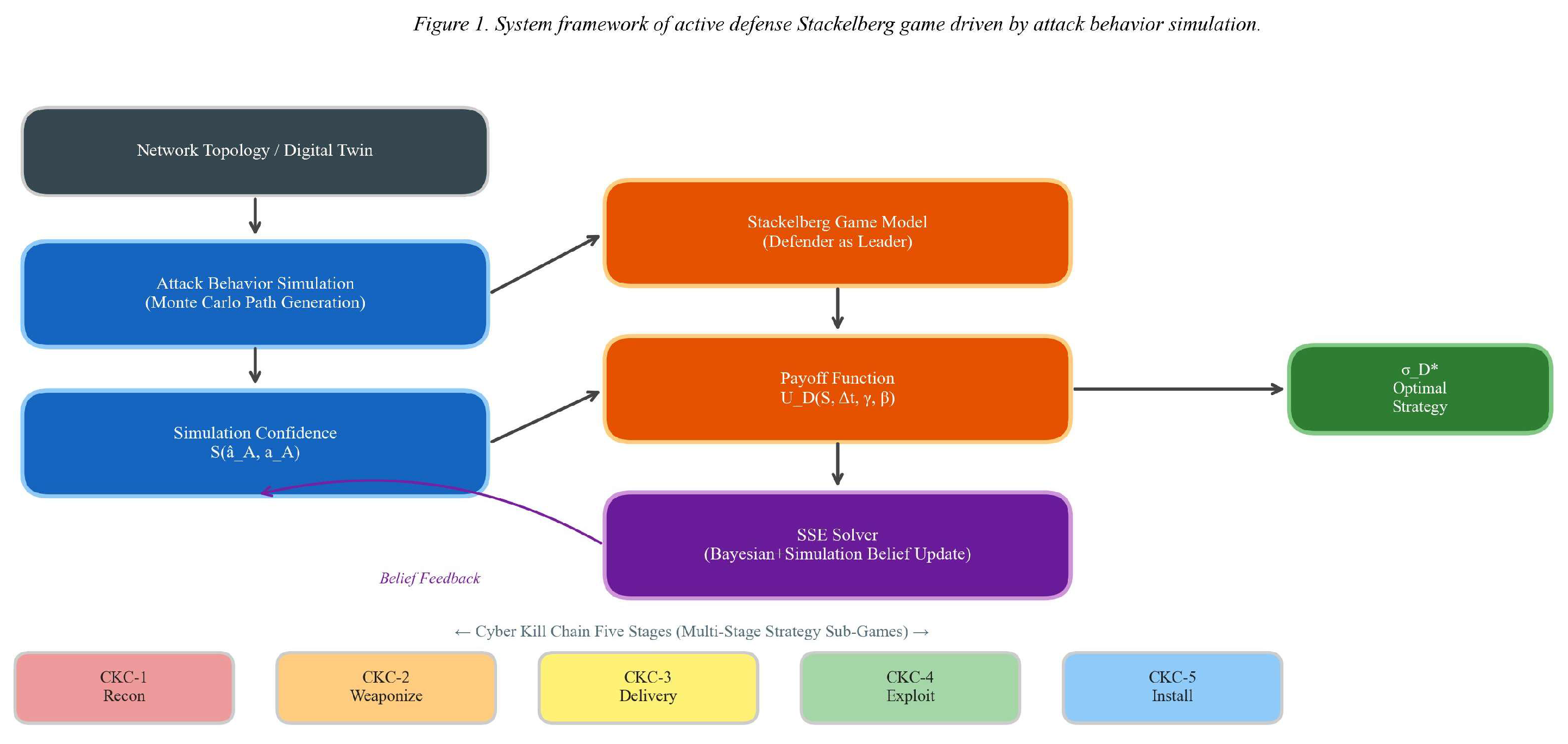
Figure 2.
Effect of simulation confidence S on comprehensive defense payoff U_D (parameters: V_D=10.0, λ=0.35, μ=0.10, β=0.05).
Figure 2.
Effect of simulation confidence S on comprehensive defense payoff U_D (parameters: V_D=10.0, λ=0.35, μ=0.10, β=0.05).
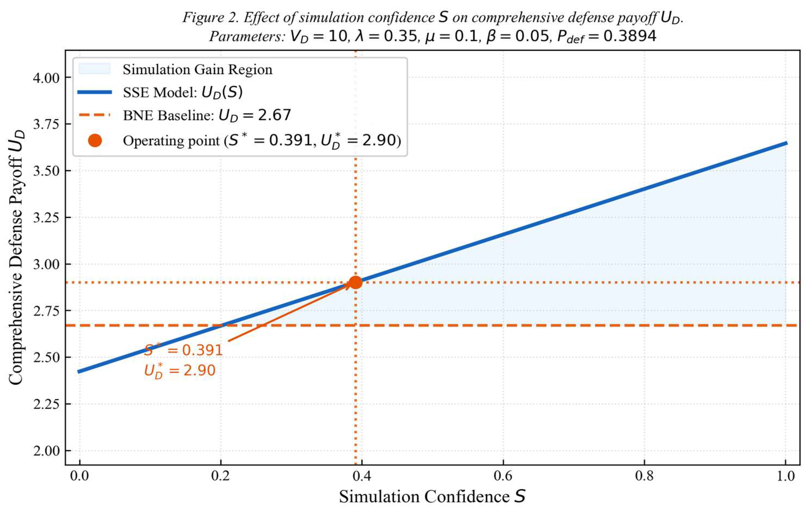
Figure 3.
Effect of response latency Δt on defender payoff U_D across five defense methods.
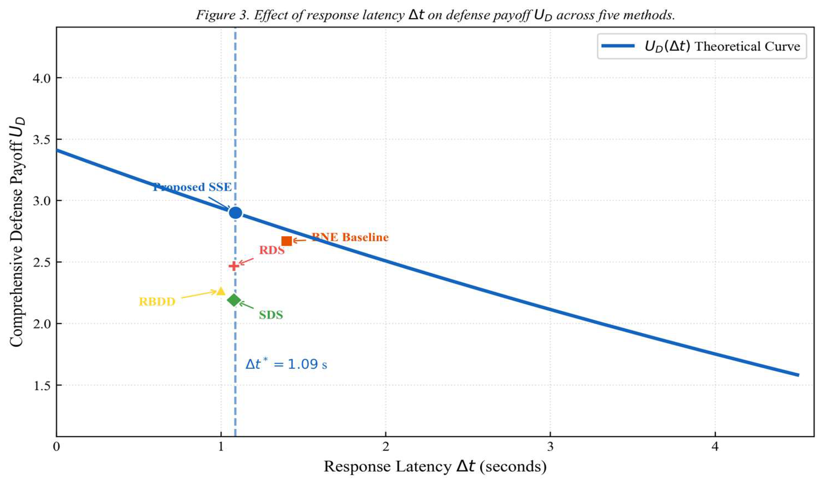
Figure 4.
Convergence curves of SSE and BNE algorithms; Nash distance d^t (log scale) vs. iteration number.
Figure 4.
Convergence curves of SSE and BNE algorithms; Nash distance d^t (log scale) vs. iteration number.
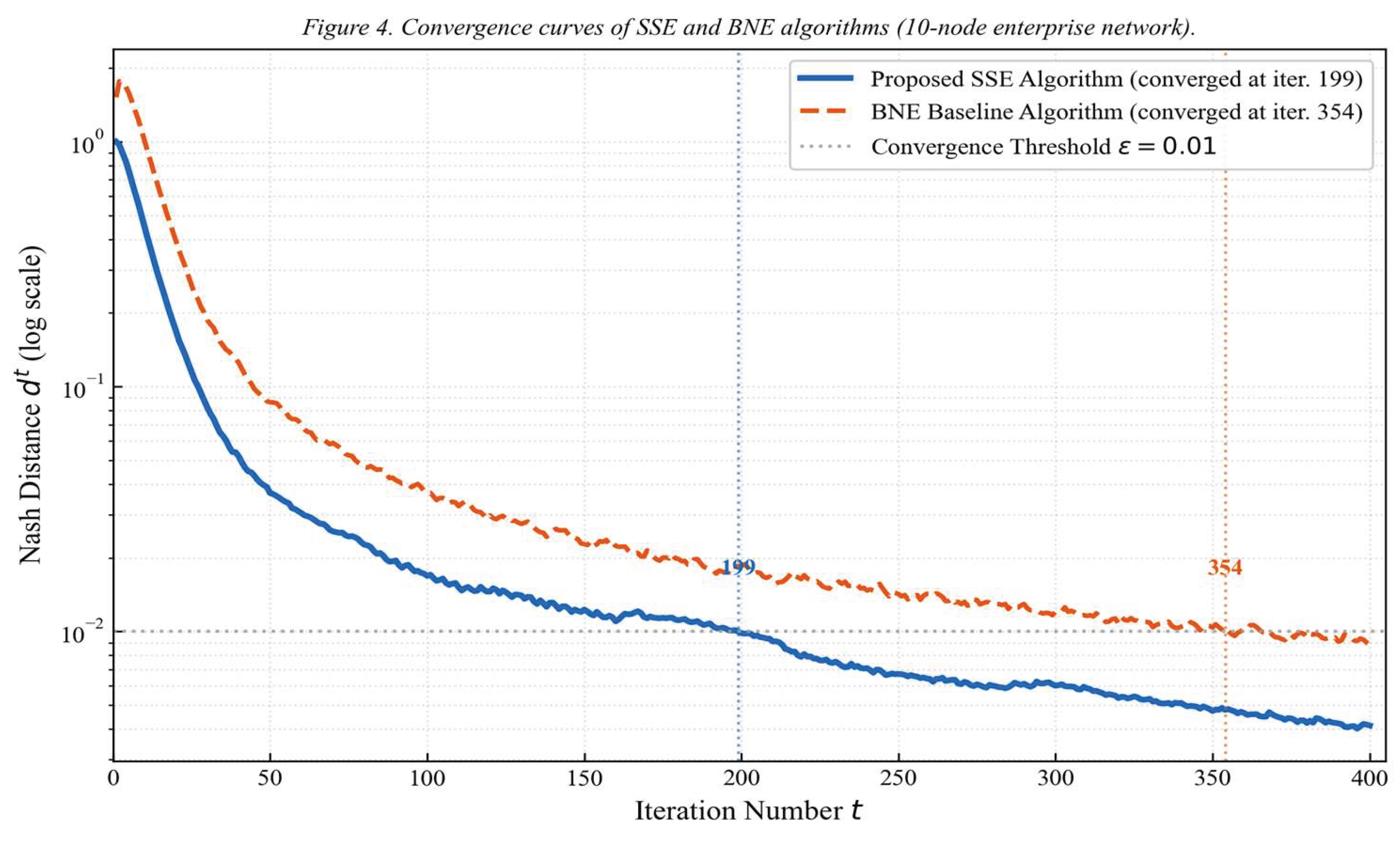

Table 1.
Model parameters and baseline values.
| Parameter | Symbol | Value | Description |
| Asset value (defender) | V_D | 10.0 | Normalized monetary/operational value of protected asset |
| Simulation amplification | λ | 0.35 | Payoff gain per unit simulation confidence |
| Latency decay coefficient | μ | 0.10 | Exponential rate of payoff decay with response delay |
| Latency penalty | β | 0.05 | Linear cost per second of response delay |
| Temporal discount factor | γ | 0.92 | Stage-to-stage payoff discount (per CKC stage) |
| Max behavioral divergence | d_max | 1.0 | Normalization bound for confidence computation |
| Simulation trials per stage | N | 1000 | Monte Carlo iterations per CKC stage |
| Convergence threshold | ε | 0.01 | Nash distance termination criterion |
| Belief smoothing factor | ε_b | 0.05 | Dirichlet smoothing for belief update stability |
Table 2.
Performance comparison across defense methods (10-node network, N=30 trials).
| Method | U_D | Δt (s) | Iterations | P_def (%) |
| Proposed SSE | 2.90 | 1.09 | 199 | 38.9 |
| BNE Baseline | 2.67 | 1.40 | 354 | 43.3 |
| RBDD | 2.27 | 1.00 | N/A | 35.6 |
| SDS | 2.19 | 1.08 | N/A | 35.9 |
| RDS | 2.47 | 1.08 | N/A | 38.5 |
Table 3.
Sensitivity of U_D to simulation amplification factor λ and discount factor γ.
| λ | γ = 0.85 | γ = 0.90 | γ = 0.92 | γ = 0.95 |
| 0.10 | 3.30 | 3.23 | 3.20 | 3.16 |
| 0.20 | 3.46 | 3.39 | 3.36 | 3.31 |
| 0.35 | 3.69 | 3.62 | 3.59 | 3.54 |
| 0.50 | 3.93 | 3.85 | 3.82 | 3.77 |
Disclaimer/Publisher’s Note: The statements, opinions and data contained in all publications are solely those of the individual author(s) and contributor(s) and not of MDPI and/or the editor(s). MDPI and/or the editor(s) disclaim responsibility for any injury to people or property resulting from any ideas, methods, instructions or products referred to in the content. |
© 2026 by the authors. Licensee MDPI, Basel, Switzerland. This article is an open access article distributed under the terms and conditions of the Creative Commons Attribution (CC BY) license.
Copyright: This open access article is published under a Creative Commons CC BY 4.0 license, which permit the free download, distribution, and reuse, provided that the author and preprint are cited in any reuse.


