

Submitted:
07 July 2026
Posted:
09 July 2026
You are already at the latest version
Abstract
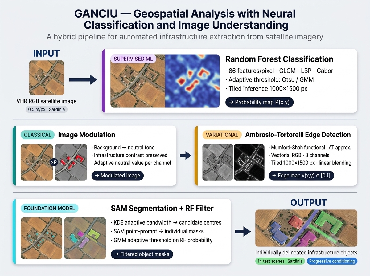
Accurate and up-to-date knowledge of land use and land cover represents one of the central challenges in spatial planning and landscape sciences. In this context, the present work introduces GANCIU (Geospatial Analysis with Neural Classification and Image Understanding), an original hybrid pipeline for the automatic extraction of man-made infrastructure from high-resolution satellite imagery. The primary methodological contribution lies in the sequential integration of four technologically heterogeneous components: a per-pixel Random Forest classifier, a guided image modulation step, edge detection via the Mumford-Shah variational functional solved through the Ambrosio-Tortorelli approximation, and final object delineation via the Segment Anything Model (SAM). Each component does not operate independently but conditions and informs the next: the RF probability map guides the modulation, which in turn directs the sensitivity of the variational step exclusively towards regions of interest; the AT edges provide spatial prompts to SAM, whose masks are finally filtered by the RF probability in an adaptive manner through a Gaussian mixture model. This progressive conditioning scheme constitutes the architectural core of GANCIU and distinguishes it from approaches that combine classification and segmentation in parallel or in purely sequential fashion without informational feedback between steps. The pipeline was applied to fourteen study areas located in Sardinia, a region characterized by a complex rural matrix and marked chromatic and geometric heterogeneity of surface types. The results reveal three distinct behavioral regimes as a function of scene difficulty: in scenes with clear radiometric contrast between infrastructure and agricultural background, the pipeline discriminates effectively at the first step; in scenes of intermediate difficulty, the AT+SAM+filter combination demonstrates a significant recovery capacity with respect to the uncertainty of the initial RF map; in scenes with dense agricultural texture, the current limitations of the training model emerge, with false positives on intensive crops representing the primary target for future development. A quantitative comparison with established methods, based on standard metrics including Precision, Recall, F1-score and Intersection over Union, is deferred to a subsequent evaluation that will extend the analysis to different geographical and sensor contexts.
Keywords:
land use land cover
; OBIA
; random forest
; Mumford-Shah
; Ambrosio-Tortorelli
; segment anything model
; remote sensing
; Sardegna
1. Introduction
Accurate and detailed knowledge of Land Use and Land Cover (LuLc) is one of the most significant areas of interest in spatial planning and landscape science. It inherently involves diverse research fields, from the strictly ecological to the technological [1,2], and holds central importance in a wide range of studies and applications. These include urban planning, natural and environmental resource monitoring, land-use policy development, and even in understanding global climate evolution [3]. Algorithmic approaches to the problem of object recognition in images (trees, rivers, roads, and other features) for LULC purposes can be traced back to two paradigms (Fig. 1): the first is structured around the analysis of the spectral signature of each individual pixel; the second, more recent and referred to as OBIA [4], involves a preliminary segmentation of the image into homogeneous regions (objects) corresponding to real-world entities, distinguishing them from what might be defined as "background" or background noise characterized by the classic "salt-and-pepper" texture [5]; these regions are subsequently subjected to semantic classification based not only on the spectral characteristics of the objects themselves, but also on their shape, texture, and spatial context [6].
Figure 1.
Conceptual diagram comparing the pixel-based and OB IA paradigms.
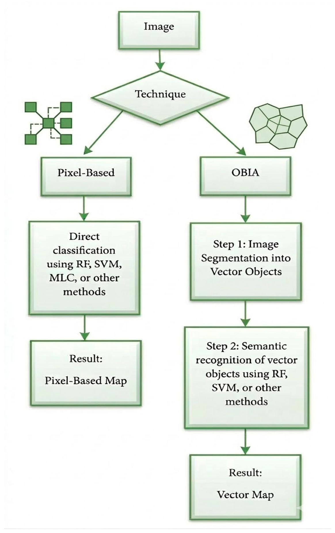
Comparative studies have demonstrated that OBIA outperforms pixel-based methods in terms of accuracy, particularly when high-resolution imagery is used and complex categories are to be classified, such as those encountered in urban environments [7]. However, this is not a matter of "right or wrong" or "better or worse", but rather of fitness for purpose: the pixel-based approach is simpler, more straightforward, and often sufficient for medium-to-low resolution data where the objective is a general estimate of land cover; whereas an OBIA approach is preferable when working with very high resolution imagery, such as that acquired by unmanned aerial vehicles [8], and/or in situations where the classes to be distinguished share similar spectral signatures but differ in shape or texture. Examples include distinguishing a roof from a road [9] or differentiating between tree species, where, in some cases, texture features are more important than purely spectral ones [10].
Classification algorithms can be distinguished into: supervised or unsupervised [11] and as parametric or non-parametric [12,13]. The first distinction is based on whether a dataset is required to train the classification algorithm. In practice, supervised algorithms are provided with input data alongside the correct corresponding outputs—for instance, 'this pixel with these characteristics is grassland.' The algorithm thus learns the relationship between input and output and replicates this procedure across the entire dataset to be analysed. In contrast, unsupervised algorithms do not require a preliminary dataset for training; instead, they autonomously identify patterns, similarities, and clusters within the dataset under analysis [14].
Algorithms can further be distinguished as parametric or non-parametric. The key discriminator here is the requirement for a strong preliminary assumption about the statistical distribution of the data [12], typically assumed to be Gaussian for parametric methods. For non-parametric algorithms, these initial assumptions are unnecessary, making them considerably more adaptable in situations where in-depth prior knowledge of the analysis area is lacking [15]. These categories are not mutually exclusive but rather intersect, providing a deeper interpretative framework for the tools. In this sense, we can identify algorithms that are: Supervised Parametric, Supervised Non-Parametric, Unsupervised Parametric, and Unsupervised Non-Parametric (see Table 1).
From the foregoing, and as can be observed in Table 1, there exists a wide variety of technological solutions that differ significantly from one another. However, there is still no single ideal or universally superior algorithm in terms of robustness and result accuracy [16]. In other words, there is no perfect algorithm, only the one most suited to a specific problem, dataset, user skill level, and final objective, in line with the "No Free Lunch Theorem" formulated by Wolpert in 1995 [17,18]. This principle implies that an algorithm's superiority only emerges in specific contexts, as its performance results from a trade-off between bias, variance, and computational complexity [19]. Consequently, the relative performance of algorithms is strictly dependent on the nature of the dataset, the size of the training set, and the specific characteristics of the thematic classes to be distinguished [20].
A detailed examination of various segmentation algorithms and their applications is provided in the edited volume by Blaschke et al. (2008) [6], which compiles several pioneering works in the field. It delves into the theoretical foundations of segmentation and the concept of scale within the principal and most widely used algorithms. A thorough exploration and classification of these would warrant a dedicated discussion, however, a sufficiently general synthesis can be attempted, starting from the seminal and foundational research by Haralick & Shapiro (1985) [21], which categorises these algorithms into logical families based on their operating principles (Figure 2).
The first family comprises algorithms that operate on the direct detection of edges (Edge Detection), identifying them where a significant gradient in brightness/colour is measured. For instance, Jin & Davis (2005) [22] utilised techniques from this family to identify building outlines using high-resolution imagery, demonstrating the utility of these algorithms within an OBIA workflow for land analysis (Figure 3A).
The second family (Region Growing) includes algorithms that function in a diametrically opposite manner to the former. Instead of seeking edges, they directly seek homogeneous areas. More specifically, they start from a 'seed pixel' and iteratively aggregate adjacent pixels that meet a similarity criterion, for example, a spectral difference below a certain threshold (Figure 3B). A valid and widespread example of this family is the Multiresolution Segmentation developed by Baatz & Schäpe (2000) [23], which simultaneously considers spectral and shape similarity.
A third family incorporates clustering techniques that group pixels based on statistical parameters. For example, the K-Means algorithm [24,25], despite its simplicity, remains a benchmark for this technique, although it requires the a priori definition of the number of clusters (K). A more robust and non-parametric evolution is represented by the Mean-Shift algorithm [26], which automatically determines the number of clusters by seeking the modes in the dataset's density distribution (Figure 3C).
The last category encompasses more modern and specialised algorithms. These develop techniques to model the physical properties of the scene, such as illumination or reflectance, to separate objects. Others are based on Graph-Based approaches (Figure 3D), which represent the image as a graph where nodes are pixels and edges connect neighbours; similarity between pixels is assigned to the edge as a weight attribute, and segmentation occurs by removing edges with minimal weight, thereby partitioning the graph [27,28].
Also, within this last family, one finds techniques based on Mixture Models, which assume the data is generated from a mixture of statistical distributions, where each mixture component represents an image region with distinct statistical properties [29].
Of course, from 1985 to the present day, theoretical and technological progression has made significant advances, and the kaleidoscope of algorithms has grown considerably. For example, Pal & Ghosh (1992) [30] explicitly acknowledge the role of fuzzy set theory in segmentation; subsequently, Cheng et al. (2001) [31] focus on colour image segmentation, incorporating specific methods, such as those based on colour physics, separating reflectance components from illumination to achieve segmentation more robust to changes in light, shadows, and reflections.
Furthermore, the advent of Deep Learning has revolutionised the playing field, developing methods capable of learning hierarchical features according to neural network architectures (e.g., FCN, U-Net), marking a significant leap forward in performance (Garcia et al., 2017) [32]. For conceptual accuracy, Deep Learning technology, like Fuzzy logic or Graph Theory itself, could be considered as transversal tools, potentially applicable to all classical segmentation families, rather than as criteria for generating new families. For instance, one could operate with a Region-Based approach, automated via a convolutional neural network that incorporates Fuzzy logic.
An additional class of tools can be identified in variational methods or energy-based models. This class distinguishes itself from the previous ones through its more strictly mathematical and geometric approach to the segmentation problem. Its seminal representative can be found in the Mumford-Shah functional [33]. Through energy optimisation, it allows the image to be segmented into homogeneous regions by differentiating its pixels into those belonging to a "smooth" zone, such as the interior of a sought-after object or the image background, and those identifying the separation, or more precisely, the boundary between objects and background. The technique of image segmentation via this procedure occurs by minimising the energy value produced by the pixels of an image (Figure 4). However, minimising the Mumford-Shah functional directly is highly complex because the set of object boundaries can have wide variability. Minimising the functional means finding the best segmentation of an image that balances three objectives [34]:
- having smooth regions, inside of which there are no large variations in the image; thus, low variance between pixel values.
- having boundaries that are as short and regular as possible.
- the processed image, where pixels are classified as boundary or background, must resemble the original image as closely as possible.
In more formal terms, for an original two-dimensional image , one seeks an image that simplifies and a set of boundaries , which minimise the overall energy as in the following (equation 1):
The first part of the equation, known as the regularity term, "penalises" variation within the smooth regions. In other words, the simplified image should be as uniform as possible inside each region, such as the interior of an object or the background itself.
The second term controls the fidelity, or more precisely, the similarity between the original image and its simplified copy , through the tuning parameter . Assuming a high value for this parameter forces the objects in the copy to be characterised by a high level of detail. However, this inevitably leads to an increase in the length of the segmentation boundary and, consequently, in the overall energy value .
Finally, the last part of the functional penalises overly long and complex boundaries through the parameter . Increasing this parameter produces solutions with shorter and simpler contours [35], but conversely, there is a risk of losing useful details that are not merely "noise."
The original formulation of the problem by Mumford and Shah stipulates that must be a finite union of closed, regular (more precisely, analytic) curves. However, as is customary in modern Mathematical Analysis, it is preferable to work with a version where such regularity is not directly required. One can then attempt to prove that the minimising sets are, in fact, more regular, using their minimality to demonstrate this. For generic sets , the concept of length can be generalised using one-dimensional Hausdorff measure. With this nuance, for each fixed , the functional can be minimised with respect to the variable in a classical manner, using appropriate Sobolev spaces, to obtain minimisers . The subsequent minimisation—that is, minimising with respect to —is more complex and requires considering the Hausdorff convergence of sets and the minimality properties of the solution [36]. Solving minimisation problems involving the Mumford-Shah functional in the presented form is therefore extremely complex, as it involves two variables, the function and the set , of very different natures.
A completely different viewpoint is due to De Giorgi [37,38], who interprets the variable as the sole variable of the problem, with the set replaced by the set of essential discontinuity points of . To implement this approach, appropriate spaces of Special functions of Bounded Variation (from which the acronym SBV is derived) were introduced and studied. Using these, the functional can be defined as follows (equation 2):
This represents the weak form of the Mumford-Shah functional, where is replaced by and a suitable meaning is given to the "approximate gradient," allowing for the resolution of the related minimisation problems. Furthermore, regularity theorems then ensure that can be considered as a union of curves [33,34,39]. Despite this conceptual effort, the implementation of a direct numerical minimisation of the Mumford-Shah functional—even via the De Giorgi [37,38] method—still presents significant difficulties. These stem from its dependence on the unknown one-dimensional set , whether considered as an arbitrary closed set or as a finite union of closed curves. However, the formulation in terms of SBV functions allows the functional to be framed within a variational setting. In this setting, one can construct approximations capable of guaranteeing the convergence of the minimisation problems, understood as the convergence of both the minimal values and the minimising functions. A sequence of functionals possessing this property is said to Gamma-converge to [40]. This approach offers greater flexibility, which translates into the possibility of developing approximations in spaces different from that of the Gamma-limit—in our case, the Mumford-Shah functional in its weak form [41].
The GANCIU (Geospatial Analysis with Neural Classification and Image Understanding) pipeline implements a four-step workflow that combines a supervised Random Forest (RF) classifier, the Mumford-Shah functional minimized through the Ambrosio-Tortorelli (AT) approximation, and the Segment Anything Model (SAM) to extract and delineate man-made infrastructure objects from very-high-resolution satellite imagery. The four steps are executed in sequence: (1) per-pixel probabilistic classification via RF, (2) image modulation guided by the RF probability map, (3) edge detection via AT applied to the modulated image, and (4) object delineation via SAM conditioned on the AT edge map, with final selection based on RF probability.
2. Methods
The following subsections describe each step-in detail, including the mathematical formulation, the parameter calibration strategy, and the computational implementation.
2.1. Per-Pixel Classification with Random Forest
The first step produces a continuous probability map P(x,y) ∈ [0,1] over the input image, where values close to 1 indicate pixels likely belonging to an infrastructure object (building, road, or other man-made structure) and values close to 0 indicate background (vegetation, bare soil, water). This is accomplished by a Random Forest classifier [42] trained on a set of manually annotated image/ground-truth pairs. The Random Forest (RF) classifier an ensemble method that generates multiple decision trees from randomly selected subsets of training samples and features [42,43] has established itself as one of the most effective and widely used algorithms for image analysis from satellite data. Its robustness to overfitting, its capacity to handle high-dimensional feature spaces, and its relative insensitivity to noisy input data make it particularly well suited to the spectral and textural complexity of high-resolution imagery [43].
In the context of the GANCIU pipeline, the RF classifier is applied at the pixel level to a set of 86 features per pixel, including multi-scale texture descriptors derived from the Gray-Level Co-occurrence Matrix (GLCM) [44], Local Binary Patterns (LBP) [46], and Gabor filters [47] at four frequencies and four orientations, alongside chromatic and gradient features. The resulting per-pixel probability map guides the subsequent segmentation stage, acting as a spatial prior that directs the variational algorithm towards regions of genuine interest and away from spectrally homogeneous background areas.
The features are designed to be invariant to absolute reflectance levels, and therefore to seasonal variation, atmospheric correction differences, and illumination changes, by relying exclusively on local statistics and relative spectral relationships. The feature set consists of four groups:
- Gray-Level Co-occurrence Matrix (GLCM) features [44] encodes the spatial co-occurrence statistics of pixel intensity values. For each of four window sizes (3, 7, 15, and 31 pixels), four Haralick descriptors are computed: contrast, homogeneity, energy, and correlation. This yields 16 features capturing texture at multiple spatial scales, from sub-metric grain to building-block level.
- Local Binary Pattern (LBP) [45] features encode the local micro-texture around each pixel by comparing it to its neighbours on a ring of radius 2 (16 sampling points, uniform patterns). Three statistical summaries — entropy, energy, and uniformity — are computed independently on each of the three RGB channels (R, G, B), yielding 9 features. The per-channel computation preserves chromatic texture information that would be lost by grayscale conversion.
- Gabor filter bank [46] at 4 frequencies (0.05, 0.15, 0.30, 0.45 cycles/pixel) and 4 orientations (0°, 45°, 90°, 135°) captures directional frequency content characteristic of structured surfaces such as rooftops and road surfaces. The mean filter response energy is computed for each of the 16 filter combinations, yielding 16 features. To capture both fine and coarse structure, the full set is duplicated across two spatial resolution levels, resulting in 32 Gabor features in total.
- Chromatic and gradient features, two relative colour ratios (R/G and the variance of the normalised RGB vector) encode spectral properties without dependence on absolute brightness. Two gradient features (gradient magnitude and the ratio of horizontal to vertical gradient) encode local structural orientation. These four features complete the 86-dimensional vector.
The RF model is trained using labelled pixel pairs extracted from a set of manually annotated scenes. For each training scene, positive samples are drawn from ground-truth infrastructure regions and negative samples from background regions, with a background-to-object ratio of k = 6 to account for the natural class imbalance in satellite imagery. The ensemble comprises 300 decision trees; the probability output for the positive class (infrastructure) is the fraction of trees that vote for that class.
At inference time, the full input image is processed in non-overlapping tiles of 1000 × 1500 pixels with a 64-pixel overlap border. The overlap border is used for feature extraction (to avoid boundary artefacts in texture filters with large kernels) but discarded before assembling the probability map. For a typical image of 6000 × 4000 pixels this tile strategy reduces peak memory consumption from approximately 7.8 GB to approximately 2 GB per tile. After assembling the full probability map, a binarisation threshold is computed adaptively from the distribution of P(x,y) using Otsu's method [47]. If the Otsu quality criterion η < 0.5 (indicating a flat, poorly bimodal distribution), the threshold is re-estimated using a two-component Gaussian Mixture Model (GMM) [48], taking the intersection of the two fitted Gaussians as the decision boundary.
Two files are produced by this step: (i) *_probabilita.tif, (Figure 5) the continuous probability map in float32 format; and (ii) *_analisi.json, a JSON file containing the statistical description of the probability distribution in the background, object, and ambiguous zones, including the optimal neutral colour values used in the following step.
2.2. Image Modulation
The second step produces a modulated version of the input image that suppresses spectral variability in background regions while preserving it in infrastructure regions. This modulated image is the input to the AT functional in the next step. The motivation is to prevent the variational algorithm from detecting edges in low-probability zones (vegetation texture, crop boundaries, shadow edges), directing its sensitivity exclusively towards regions indicated by the RF classifier as likely infrastructure. For each pixel (x, y) and each colour channel c ∈ {R, G, B}, the modulated image value is computed as:
Where is the original pixel value in channel c; is the RF probability map; is the neutral value for channel c; and γ is a user-controlled modulation curve parameter (default γ = 1.0, corresponding to a linear transition). The neutral value is determined adaptively for each image from the statistical analysis produced in Step 1: it is chosen as the median (or mode, if the distribution is strongly skewed) of pixel values in channel c within the background zone where t is the Otsu threshold. This ensures that background pixels converge to a radiometrically appropriate flat colour rather than an arbitrary constant. The parameter γ controls the sharpness of the transition between preserved and suppressed regions:
- γ = 1.0 (default): linear transition — a pixel with P = 0.5 receives equal weight from original and neutral.
- γ < 1.0 (e.g., 0.5): soft transition — more of the original signal is preserved at intermediate probabilities.
- γ > 1.0 (e.g., 2.0): hard transition — intermediate probabilities are pushed strongly towards the neutral value
The modulated image is saved as *_modulata.tif (uint8, 3 bands)
Statistics (mean, standard deviation, 75th and 90th percentiles) are extracted from pixels within the high-probability RF zone P(x,y) > t, so that gradient statistics refer to genuine infrastructure edges rather than background noise. The three AT parameters are then set as:
- μ = clip(0.05/ḡ, 0.1, 10.0), where ḡ is the mean gradient magnitude in the RF zone. This scales the data-fidelity term relative to the actual contrast present in the scene.
- ν = μ/1000. The contour-length penalty is kept proportional to μ to maintain a consistent balance between regularisation and fidelity across scenes.
- ε schedule: a decreasing sequence of ε values is selected from three pre-defined schedules (short, medium, long) based on the scene difficulty index — defined as the fraction of ambiguous pixels relative to the fraction of RF-positive pixels. Harder scenes use longer schedules that start from larger ε values (e.g., [4.0, 2.0, 1.0, 0.5, 0.2, 0.1, 0.05, 0.02, 0.01]) to ensure convergence.
The calibrated parameters are stored in *_parametri_AT_su_modula.json and read automatically by next step.
2.3. Edge Detection via Ambrosio-Tortorelli
The third step applies the Ambrosio-Tortorelli (AT) approximation of the Mumford-Shah functional to the modulated image, producing a continuous edge map v(x,y) ∈ [0,1] in which low values identify strong discontinuities (edges) and values close to 1 correspond to smooth interior regions. Among the various solutions for numerically approximating the Mumford-Shah functional, the one proposed and studied by Ambrosio and Tortorelli has been particularly widely used, especially in computational contexts [49]. The core idea behind this approximation is the use of an additional variable or parameter: a function , such that is a "regularised" version of the characteristic function of the discontinuity set . In essence, the function takes the value 1 "far" from the discontinuity set of , and 0 "close" to it. The "regularized" term is:
is thus well-defined even if the function u is discontinuous on S(u), meaning that over this set the product with v2 is null. The term involving the length of S(u) is replaced with a continuous approximation dependent on the parameter n, with n tending to infinity:
For large n, the finiteness of the first term in this integral implies that v is close to the constant 1 except on a set of small measures. Recalling that the value of v is 0 on S(u), this means the function v must undergo a transition from 0 to 1 in a neighbourhood of S(u). This transition, however, is penalised by the second integral. As n tends to infinity, these two terms balance each other, and their combined value tends to a multiple of the length of S(u), due to a Gamma-convergence result related to phase transitions [50].
The Ambrosio-Tortorelli functional, dependent on the parameter n, thus takes the overall form:
Following the solution proposed by Ambrosio and Tortorelli, we must find the function (the approximated image) and the function (the edge map) that minimise the value of . The numerical implementation follows these logical steps (Figure 6):
- a)
- Initialisation:
- ∙
- A matrix u(x,y) is created to approximate the original image g(x,y) as closely as possible. The ideal initial solution is therefore to initialise u(x,y) with the exact numerical values of g(x,y).
- ∙
- For the function v, which will contain the edge map, a matrix of the same dimensions as u(x,y) is initialised, with all its elements assigned the value v=1. Starting with the value 1 everywhere means assuming, in the initial phase, that there are no edges in the image—a neutral starting hypothesis. In subsequent iterations, the algorithm will update this matrix, pushing values towards the threshold 0 to identify discontinuities (i.e., the edges of the sought objects).
b) Iterative Minimisation; once the matrix is initialised, the functional is minimised through an iterative process:
- ∙
- Minimise with respect to u: The values in the matrix u(x,y) are updated, using the current v matrix (initially all 1s).
- ∙
- Minimise with respect to v: Using the newly computed u(x,y) matrix from the previous step, the functional is minimised again, this time with respect to v. This yields an updated edge map matrix v.
c) Convergence: these alternating minimisations between the and matrices are repeated until the changes in the respective updated matrices are deemed negligible.
Specifically, the minimisation of u(x,y) with respect to v is implemented via the Euler–Lagrange equation for u (in discrete form), which yields a linear system whereby each element of the matrix u(x,y) is updated as a function of its neighbours. For each pixel, a new value is then computed, balancing the original datum and the regularisation term:
where *h* is the spatial step (h=1) and, in the case of the first iteration where v=1 everywhere, the expression simplifies to an average between the datum and the mean of its neighbours. Conversely, for the minimisation of v with respect to the updated u(x,y), the formula derived from the per-pixel minimisation of the matrix is used:
where the squared magnitude ∣∇u∣2 is obtained using the centered finite-difference scheme to compute the partial derivatives:
It should be recalled that in regions where the gradient is high, v becomes small (<<1), allowing u(x,y) to approach the original data more closely in subsequent iterations. Direct application of the AT algorithm to full-resolution images (6000 × 4000 pixels or larger) is computationally intractable on standard hardware. The image is therefore partitioned into tiles of 1000 × 1500 pixels with an overlap border of 128 pixels. Each tile is processed independently; in the overlap zones, results from adjacent tiles are blended using a linearly increasing weight ramp (from 0 at the tile edge to 1 at the interior boundary). This weighted blending prevents discontinuities in the edge map at tile boundaries, which would otherwise produce artefacts in the subsequent SAM step. The output of this step is *_modulata_v_map.tif: a float32 raster with values in [0,1] (Figure 7).
2.4. Object Delineation via SAM
A further contribution to the object delineation stage comes from the Segment Anything Model (SAM) [49], a foundation model developed by Meta AI and trained on over one billion segmentation masks. SAM operates through a promptable architecture: given a point, bounding box, or other spatial cue, it generates a precise segmentation mask for the corresponding object with zero-shot generalization across image types and domains. Its application to remote sensing imagery has been systematically evaluated, demonstrating strong performance in delineating buildings, roads, and infrastructure from aerial and satellite data, particularly when combined with an upstream classifier providing candidate object locations. In the workflow presented here, SAM receives point prompts derived from the density peaks of the AT edge map and produces individual object masks that are subsequently filtered by the RF probability map, retaining only those objects whose interior pixels exhibit high classification confidence.
The fourth step converts the continuous AT edge map into discrete, individually segmented object masks using the Segment Anything Model (SAM) [51]. The process involves three sub-steps: identification of candidate object centres from the edge map, generation of SAM masks via point prompts, and filtering of masks by RF probability. The AT edge map is first inverted: the boundary strength signal is defined as b(x,y) = 1 − v(x,y), so that strong edges correspond to high values. Pixels with b < 0.05 are considered inactive and excluded from further processing. To identify individual object locations, a spatial Kernel Density Estimation (KDE) is applied to the active edge pixels. The KDE bandwidth is set adaptively as three times the mean nearest-neighbour distance among active edge pixels, computed via a k-d tree. The resulting density map is smoothed with a Gaussian filter of the same bandwidth. Local maxima of the density map (peaks separated by at least one bandwidth radius) are taken as candidate object centres. The distribution of b values among active pixels is modelled by a two-component Gaussian Mixture Model. The intersection of the two fitted Gaussians is used as the threshold separating weak edges (likely noise or background texture) from strong edges (likely object boundaries). Only active pixels above this adaptive threshold are retained for KDE computation, ensuring that the density map responds to genuine structural boundaries rather than residual background signal (Figure 8).
For each candidate centre identified by the KDE, SAM is queried with a single point prompt at the centre coordinates. SAM generates multiple candidate masks for each prompt; the mask with the highest confidence score is selected. All selected masks are kept as separate objects — no mask merging is performed at this stage, so adjacent or overlapping objects remain distinct. SAM operates on the original RGB image (not the modulated version) to preserve the full spectral contrast available for boundary delineation. The SAM model used is the ViT-B variant (vit_b), which provides an optimal balance between segmentation accuracy and inference speed for large satellite images.
Not all SAM-produced masks correspond to genuine infrastructure objects: some may arise from vegetation clusters, shadows, or other high-contrast features that were not fully suppressed by the modulation step. Each mask is filtered by computing the mean RF probability over its interior pixels:
where Sm is the set of pixels belonging to mask m; the distribution of P̄_m values across all masks is again modelled by a two-component GMM. Only masks in the high-probability component ( above the GMM intersection) are retained as confirmed infrastructure objects. This adaptive threshold — rather than a fixed cutoff — automatically adjusts to the difficulty and scene-specific probability range of each image. Three diagnostic images are produced at the end of Step 4: (i) *_bordi_su_rgb.jpg, showing the strong-edge pixels overlaid in red on the original RGB; (ii) *_kde_centroidi.jpg, showing the KDE density peaks with their estimated radius overlaid as cyan circles; and (iii) *_SAM_separati.jpg, showing the final filtered SAM masks in randomly assigned colours on the original RGB (Figure 9).
All processing was carried out in Python 3.11 using NumPy, SciPy, scikit-image, scikit-learn, and rasterio. SAM inference used PyTorch.
3. Experiment and Results
Sardinia is the second largest island in the Mediterranean, with an area of approximately 24,000 km2, and represents one of the most strongly rural regions in the whole of Italy. This characteristic is not simply the result of a superficial reading of the territory: several analytical models applied to the island converge in confirming its predominantly rural character, rooted in a long agro-pastoral tradition that has shaped, over the centuries, not only the economy but also the cultural and landscape identity of the region. This apparently solid picture, however, conceals worrying dynamics. Rural Sardinia is today a reality in profound transformation, caught between the crisis of the primary sector and the rise of new economies that are reshaping land use across the island: the emergence of tourism as a new economic driver is significantly altering the rural character of the island, exerting growing pressure on coastal areas, where demand for buildable land for hospitality purposes directly competes with agricultural and natural land uses [52]. Having tools that allow continuous and as accurate as possible monitoring of anthropogenic pressures and changes in land cover and land use is the foundation for structuring territorial planning models that are coherent with the evolution of the context. However, the challenges involved in developing such tools are far from negligible, due primarily to the complexity of certain territorial contexts [53]. The intrinsic difficulty of computer vision algorithms in correctly interpreting image content stems mainly from the presence of noise and perturbations, which can lead to instability and poor-quality reconstructions [54], as well as from the inevitable yet cyclical seasonal change affecting certain rural and environmental contexts [55] (Figure 10).
In this experimental section, we present the results obtained from the application of GANCIU to fourteen study areas characterised by varying levels of geometric and chromatic complexity of surface types. Residential anthropogenic surfaces may appear as small isolated dwellings or as more structured residential urban clusters; similarly, agricultural holdings may consist of a single warehouse or more complex structures, typically with roofing in metallic materials or, in the case of intensive horticultural greenhouses, in iron-and-glass construction. Road infrastructure is represented by surfaced high-speed roads, provincial roads, and unpaved agricultural access tracks. The agricultural and environmental matrix surrounding the anthropogenic surfaces may present itself as bare soil with no vegetation cover during the summer period, or covered by grass during the spring season, or display recurring geometric and chromatic patterns such as rows of vineyards or olive groves, or alternatively be covered by forested surfaces (Figure 11).
The Random Forest produces P(object) probability maps with markedly different behaviours depending on the scene type, revealing both the strengths and the limitations of the current model. The simplest cases are test1, test4, test5, test6 and test9 — scenes featuring buildings that are well separated from the surrounding agricultural context. The Otsu threshold is high (0.37–0.41), the difficulty index is moderate (0.67–0.75), and the object percentage is limited (6–18%). The model discriminates well in these cases because the radiometric contrast between buildings and background is clear. Test9 is particularly clean despite its large extent — only 6.4% object coverage with a minimal ambiguous zone of 5%, indicating a very sharp bimodal distribution between background and infrastructure (Figure 12).
The intermediate-difficulty cases are test2, test3, test13 and test14. The latter deserves specific attention: it has a difficulty index of 1.02 with an ambiguous zone of 24.8% and a very low mean gradient (0.025) — meaning that the ambiguous zone exceeds the candidate zone itself and the model is uncertain over a very large fraction of pixels. Nevertheless, the pipeline as a whole produces a useful result: 167 objects retained out of 186, with a final RF probability threshold of 0.55. This apparently contradictory behavior — high RF uncertainty but good final confidence — suggests that the AT+SAM+filter combination recovers meaningful results even when the RF map alone is difficult to interpret, because the AT edges identify the geometric structures and SAM segments them with sufficient precision to allow the higher RF probability of buildings relative to the surrounding terrain to emerge (Figure 13).
The most challenging cases are test7 and test8. Test7 has 32.7% of pixels classified as objects and an ambiguous zone of 46.2% — almost half of all pixels fall within the uncertainty band between 0.3 and 0.7. Test8 is analogous, with 38.7% object coverage and an ambiguous zone of 46.5%. In both scenes, the low mean gradient (0.037–0.054) indicates blurred boundaries in the modulated image, a condition that complicates the work of the AT step in the subsequent processing stage (Figure 14).
Test10, test11 and test12 represent a structurally different problem: predominantly agricultural scenes with no significant buildings, in which the model assigns medium-to-high probabilities to cultivated surfaces with dense texture. In test10, 35% of the image is classified as object — an anomalous value for a scene devoid of infrastructure. This is the primary limitation of the current model: rf_model_v10 has never been exposed to sufficient examples of intensive crops as pure background, and consequently confuses the texture of row crops and arable fields with that of built infrastructure. The Otsu threshold is low (0.14–0.16) but with a separation eta that remains high (0.80–0.83), indicating that the distribution is bimodal but the two peaks correspond to different crop types rather than to background and building (Figure 15).
The modulation step performed consistently across all test cases. The percentage of significantly modified pixels ranges from 85.6% in test4 to 99.7% in test11, confirming that in almost all cases the vast majority of the image is flattened towards the neutral value. The only notable exception is test14, where the outcome is a direct consequence of the RF output: test14 has a very wide ambiguous zone and few pixels with either very high or very low probability; consequently, the modulation produces only weak suppression — most pixels are modified to a limited extent because the RF probability is concentrated in the intermediate band. The result is a modulated image with reduced contrasts, which accounts for the very low mean gradient (0.015).
In the Ambrosio-Tortorelli step, all fourteen test cases use the long epsilon schedule with max_iter=150; this is an expected outcome for rural imagery where boundaries between surface materials are often gradual rather than sharp. The parameter mu varies significantly across scenes: from 1.14 in test10 to 3.25 in test14. A high value of this parameter means that the AT is less sensitive to weak gradients and tends to produce edges only where the contrast is sharp — a necessary condition for scenes with a low mean gradient such as test7 (mu=3.03) and test14 (mu=3.25). Conversely, test10 with mu=1.14 is more sensitive (Figure 16), consistently with its higher mean gradient (0.044)
The AT processing times reflect image dimensions with an almost linear relationship: from 15 seconds for test1 (803×1186 pixels) to 460 seconds for test7 (2171×2995 pixels). Test2 (2439×2954 pixels) takes 324 seconds despite dimensions comparable to test7 — the difference is explained by test7's considerably higher mu value (3.03 vs 2.72), which requires more iterations to converge. The final v_map always has a very high mean (0.98–0.999), confirming that the vast majority of pixels constitute homogeneous background and edges occupy only a minimal fraction. The minimum v value ranges from 0.13 in test8 to 0.30 in test13 — test13 has the highest minimum, indicating that even the strongest edges have a relatively high v value, most likely because the weak modulation produced only modest gradients in the modulated image. Test8 deserves particular attention: v_min=0.131 is the lowest value in the entire dataset, alongside vmean=0.987, indicating that test8 contains the strongest and sharpest edges of all test cases.
In the final step of GANCIU (Step 4), the number of strong edge pixels varies enormously — from 1,382 in test5 (small image) to 78,704 in test8 (dense and complex scene). The KDE radius is remarkably stable across all test cases: from 3.04 to 3.59 pixels. This is an important finding — it means that regardless of image size and scene complexity, the mean distance between adjacent edge pixels is nearly constant. AT edges tend to form linear structures of similar thickness across all scenes, confirming the geometric consistency of the algorithm. When the RF probability is subsequently applied as a filter on the SAM masks, the most interesting variability emerges: the adaptive GMM threshold ranges from 0.20 in test11 to 0.86 in test5 — an extremely wide range that reflects the quality of the separation between genuine objects and false positives.
The cases with clear separation are test1 (threshold 0.765, prob_max=0.946), test5 (threshold 0.861, prob_max=0.906) and test14 (threshold 0.551, prob_max=0.917). In these cases the GMM identifies two well-separated components — genuine buildings have a high and consistent mean internal RF probability, while false positives exhibit low probability. Test14 is particularly significant: despite the RF being uncertain at Step 1, the SAM+filter combination recovers a useful separation with prob_mean=0.713, the highest value in the entire dataset (Figure 17). The cases with weak separation are test11 (threshold 0.204) and test12 (threshold 0.328). Here the GMM fails to identify a distinct high-probability component — almost all masks have a low mean RF probability because there are no genuine buildings to form a separate cluster. Test11 represents the most extreme case: prob_min=0.009 and threshold=0.204 indicate that the GMM has effectively capitulated, retaining 428 objects out of 608 that are almost certainly false positives on cultivated fields (Figure 18).
4. Discussion
The GANCIU pipeline has demonstrated its validity as an approach for the automatic extraction of man-made infrastructure from very-high-resolution satellite imagery. Its hybrid architecture — combining per-pixel classification with Random Forest, guided image modulation, edge detection via the Mumford-Shah functional solved through the Ambrosio-Tortorelli approximation, and object delineation via the Segment Anything Model — has produced internally consistent and interpretable results across fourteen study areas in Sardinia, characterised by varying levels of geometric and chromatic complexity. The qualitative analysis of the fourteen test scenes reveals three distinct behavioural regimes, reflecting the intrinsic difficulty of the classification task.
In the simplest cases (test1, test4, test5, test6, test9), where anthropogenic structures are well separated from the surrounding agricultural matrix and exhibit clear radiometric contrast, the Random Forest produced probability maps with strongly bimodal distributions and high Otsu thresholds (0.37–0.41), with difficulty indices ranging between 0.67 and 0.75. Under these conditions the pipeline discriminated infrastructure from background already at the first step, with the subsequent stages consolidating rather than correcting the initial classification.
In the intermediate-difficulty cases (test2, test3, test13, test14), the pipeline demonstrated a remarkable recovery capacity. Test14 is particularly instructive: despite an RF difficulty index of 1.02 and an ambiguous zone covering 24.8% of pixels — meaning that the ambiguous zone exceeded the candidate zone itself — the AT+SAM+RF filter combination retained 167 objects out of 186, with a mean internal RF probability of 0.713, the highest value in the entire dataset. This result suggests that the geometric precision of AT edge detection and the boundary delineation capability of SAM can compensate for an uncertain RF probability map, provided that genuine structural boundaries are present in the modulated image. The GMM adaptive thresholding mechanism, which calibrates the final filter on the scene-specific probability distribution rather than applying a fixed value, appears to be a determining factor in enabling this recovery.
The most challenging cases (test7, test8) exposed the current limitations of the system. With more than 30% of pixels classified as objects and ambiguous zones exceeding 46%, the low mean gradient in the modulated image (0.037–0.054) reduced the sensitivity of the AT step, producing edge maps with less pronounced minima. Although test8 exhibited the strongest and sharpest edges in the entire dataset (v_min = 0.131), the high density of candidate centres introduced by the KDE step increased the risk of over-segmentation.
A structurally distinct failure mode emerged in the predominantly agricultural scenes with dense texture (test10, test11, test12). In these cases the Random Forest assigned anomalously high probabilities to cultivated surfaces — in test10, 35% of the image was classified as infrastructure — while simultaneously producing a bimodal distribution (η = 0.80–0.83) whose two peaks corresponded to different crop types rather than to background and built structures. This reveals a systematic gap in the training dataset: the current rf_model_v10 has not been exposed to a sufficient number of examples of intensive agricultural surfaces as pure background. The consequences propagate throughout the entire pipeline: in test11, the GMM-based filter at Step 4 failed to identify a high-probability cluster of genuine objects, retaining 428 masks out of 608 (threshold = 0.204) that are in all likelihood false positives on cultivated fields. This represents the most critical failure mode identified in the present study and the primary target for future development.
Across all fourteen scenes, the modulation step operated consistently, suppressing between 85.6% (test4) and 99.7% (test11) of image pixels towards the neutral value. The AT parameter μ varied systematically with scene difficulty, from 1.14 (test10) to 3.25 (test14), reflecting the adaptive calibration of the data-fidelity term relative to the gradient contrast effectively available in each modulated image. Processing times scaled in an approximately linear fashion with image area, from 15 seconds (test1, 803×1186 pixels) to 460 seconds (test7, 2171×2995 pixels). The KDE bandwidth remained remarkably stable across all scenes (3.04–3.59 pixels), confirming the geometric consistency of the AT edge structure regardless of scene complexity.
It should be noted that the evaluation presented here is qualitative in nature, based on the internal statistical diagnostics produced by the pipeline at each step, rather than on comparison with a labelled ground truth using standard accuracy metrics such as Precision, Recall, F1-score and Intersection over Union. A rigorous quantitative evaluation — encompassing benchmarking against established methods such as standalone Random Forest classification, OBIA workflows based on eCognition, or deep learning segmentation architectures — is explicitly deferred to a subsequent study, which will also address the generalisation of the model to satellite imagery acquired from different sensors and in different geographical contexts. The results presented here are therefore intended to characterise the internal behaviour of the pipeline and its failure modes, providing a reasoned basis for the targeted improvements described below, rather than to establish its absolute performance relative to the state of the art.
To improve the overall precision of GANCIU, future developments are directed along three converging lines. First, the training dataset will be enriched through targeted sampling of intensive agricultural surfaces — including vineyard rows, olive groves, and greenhouse structures — supported by data augmentation techniques, with the aim of increasing the representation of spectrally ambiguous backgrounds without a proportional increase in annotation effort. Second, geometric constraints based on mask compactness and aspect ratio will be introduced in the final filtering stage, exploiting the known morphological regularity of buildings and roads to distinguish them from the elongated and periodic patterns of row crops. Third, the final filter will be reformulated to combine RF probability with shape descriptors derived from SAM, replacing the current single-criterion GMM threshold with a multi-feature decision boundary capable of separating genuine infrastructure masks from agricultural false positives even when their mean internal RF probability overlaps substantially.
5. Patents
This section is not mandatory but may be added if there are patents resulting from the work reported in this manuscript.
Author Contributions
For research articles with several authors, a short paragraph specifying their individual contributions must be provided. The following statements should be used “Conceptualization, Amedeo Ganciu; methodology, Amedeo Ganciu, Giovannangela Ricci, Margherita Solci; software, Amedeo Ganciu; validation, Giovannangela Ricci, Margherita Solci; formal analysis, Amedeo Ganciu; investigation, Amedeo Ganciu; data curation, Amedeo Ganciu; writing—original draft preparation, Amedeo Ganciu, Giovannangela Ricci, Margherita Solci; writing—review and editing, Amedeo Ganciu; visualization, Amedeo Ganciu. All authors have read and agreed to the published version of the manuscript.” Please turn to the CRediT taxonomy for the term explanation. Authorship must be limited to those who have contributed substantially to the work reported.
Informed Consent Statement
“Not applicable.” for studies not involving humans. You might also choose to exclude this statement if the study did not involve humans.
Data Availability Statement
We encourage all authors of articles published in MDPI journals to share their research data. In this section, please provide details regarding where data supporting reported results can be found, including links to publicly archived datasets analyzed or generated during the study. Where no new data were created, or where data is unavailable due to privacy or ethical restrictions, a statement is still required. Suggested Data Availability Statements are available in section “MDPI Research Data Policies” at https://www.mdpi.com/ethics.
Conflicts of Interest
The authors declare no conflicts of interest.
References
References
- Abdi, A. M. Land cover and land use classification performance of machine learning algorithms in a boreal landscape using Sentinel-2 data. GIScience Remote Sens. 2020, 57(1), 1–20. [Google Scholar]
- Yimer, S. M.; Bouanani, A.; Kumar, N.; Tischbein, B.; Borgemeister, C. Comparison of different machine-learning algorithms for land use land cover mapping in a heterogenous landscape over the Eastern Nile River basin, Ethiopia. Adv. Space Res. 2024, 74(5), 2180–2199. [Google Scholar] [CrossRef]
- Schulz, D.; Yin, H.; Tischbein, B.; Verleysdonk, S.; Adamou, R.; Kumar, N. Land use mapping using Sentinel-1 and Sentinel-2 time series in a heterogeneous landscape in Niger, Sahel. ISPRS J. Photogramm. Remote Sens. 2021, 178, 97–111. [Google Scholar] [CrossRef]
- Duro, D. C.; Franklin, S. E.; Dubé, M. G. A comparison of pixel-based and object-based image analysis with selected machine learning algorithms for the classification of agricultural landscapes using SPOT-5 HRG imagery. Remote Sens. Environ. 2012, 118, 259–272. [Google Scholar] [CrossRef]
- Blaschke, T. Object based image analysis for remote sensing. ISPRS J. Photogramm. Remote Sens. 2010, 65(1), 2–16. [Google Scholar] [CrossRef]
- Blaschke, T.; Lang, S.; Hay, G. (Eds.) Object-based image analysis: spatial concepts for knowledge-driven remote sensing applications; Springer Science & Business Media, 2008. [Google Scholar]
- Myint, S. W.; Gober, P.; Brazel, A.; Grossman-Clarke, S.; Weng, Q. Per-pixel vs. object-based classification of urban land cover extraction using high spatial resolution imagery. Remote Sens. Environ. 2011, 115(5), 1145–1161. [Google Scholar] [CrossRef]
- Michez, A.; Piégay, H.; Lisein, J.; Claessens, H.; Lejeune, P. Classification of riparian forest species and health condition using multi-temporal and hyperspatial imagery from a unmanned aerial system. Environ. Monit. Assess. 2016, 188(3), 146. [Google Scholar] [CrossRef] [PubMed]
- Zhou, W.; Troy, A. An object-oriented approach for analysing and characterizing urban landscape at the parcel level. Int. J. Remote Sens. 2008, 29(11), 3119–3135. [Google Scholar] [CrossRef]
- Laliberte, A. S.; Browning, D. M.; Rango, A. A comparison of three feature selection methods for object-based classification of sub-decimeter resolution UltraCam-L imagery. Int. J. Appl. Earth Obs. Geoinf. 2012, 15, 70–78. [Google Scholar] [CrossRef]
- Saponaro, M.; Tarantino, E. LULC Classification Performance of Supervised and Unsupervised Algorithms on UAV-Orthomosaics. In International Conference on Computational Science and Its Applications; Springer International Publishing: Cham, July 2022; pp. 311–326. [Google Scholar]
- Qian, Y.; Zhou, W.; Yan, J.; Li, W.; Han, L. Comparing machine learning classifiers for object-based land cover classification using very high-resolution imagery. Remote Sens. 2014, 7(1), 153–168. [Google Scholar] [CrossRef]
- Phiri, D.; Morgenroth, J. Developments in Landsat land cover classification methods: A review. Remote Sens. 2017, 9(9), 967. [Google Scholar] [CrossRef]
- Lu, D.; Weng, Q. A survey of image classification methods and techniques for improving classification performance. Int. J. Remote Sens. 2007, 28(5), 823–870. [Google Scholar] [CrossRef]
- Shao, Y.; Lunetta, R. S. Comparison of support vector machine, neural network, and CART algorithms for the land-cover classification using limited training data points. ISPRS J. Photogramm. Remote Sens. 2012, 70, 78–87. [Google Scholar] [CrossRef]
- Gašparović, M.; Zrinjski, M.; Gudelj, M. Automatic cost-effective method for land cover classification (ALCC). Comput. Environ. Urban Syst. 2019, 76, 1–10. [Google Scholar] [CrossRef]
- Wolpert, D. H.; Macready, W. G. No free lunch theorems for optimization. IEEE Trans. Evol. Comput. 2002, 1(1), 67–82. [Google Scholar]
- Hastie, T.; Tibshirani, R.; Friedman, J. Model assessment and selection. In The elements of statistical learning: data mining, inference, and prediction; Springer New York: New York, NY, 2008; pp. 219–259. [Google Scholar]
- Domingos, P. A few useful things to know about machine learning. Commun. ACM 2012, 55(10), 78–87. [Google Scholar] [CrossRef]
- Maxwell, A. E.; Warner, T. A.; Fang, F. Implementation of machine-learning classification in remote sensing: An applied review. Int. J. Remote Sens. 2018, 39(9), 2784–2817. [Google Scholar] [CrossRef]
- Haralick, R. M.; Shapiro, L. G. Image segmentation techniques. Comput. Vis. Graph. Image Process. 1985, 29(1), 100–132. [Google Scholar] [CrossRef]
- Jin, X.; Davis, C. H. Automated building extraction from high-resolution satellite imagery in urban areas using structural, contextual, and spectral information. EURASIP J. Adv. Signal Process. 2005, 2005(14), 745309. [Google Scholar] [CrossRef]
- Baatz, M.; Schape, A. Multiresolution Segmentation: An Optimization Approach for High Quality Multi-Scale Image Segmentation. In Angewandte Geographische Informations-Verarbeitung; Strobl, J., Blaschke, T., Griesbner, G., Eds.; Wichmann Verlag: Karlsruhe, Germany, 2000; Volume XII, pp. 12–23. [Google Scholar]
- MacQueen, J. Some methods for classification and analysis of multivariate observations. Proc. Fifth Berkeley Symp. Math. Stat. Probab. 1967, 1(14), 281–297. [Google Scholar]
- Hartigan, J. A.; Wong, M. A. Algorithm AS 136: A K-means clustering algorithm. J. R. Stat. Soc. Ser. C (Applied Statistics) 1979, 28(1), 100–108. [Google Scholar] [CrossRef]
- Comaniciu, D.; Meer, P. Mean shift: A robust approach toward feature space analysis. IEEE Trans. Pattern Anal. Mach. Intell. 2002, 24(5), 603–619. [Google Scholar] [CrossRef]
- Shi, J.; Malik, J. Normalized cuts and image segmentation. IEEE Trans. Pattern Anal. Mach. Intell. 2000, 22(8), 888–905. [Google Scholar] [CrossRef]
- Felzenszwalb, P. F.; Huttenlocher, D. P. Efficient graph-based image segmentation. Int. J. Comput. Vis. 2004, 59(2), 167–181. [Google Scholar] [CrossRef]
- McLachlan, G. J.; Peel, D. Finite mixture models; John Wiley & Sons, 2000. [Google Scholar]
- Pal, S. K.; Ghosh, A. Image segmentation using fuzzy correlation. Inf. Sci. 1992, 62(3), 223–250. [Google Scholar] [CrossRef]
- Cheng, H. D.; Jiang, X. H.; Sun, Y.; Wang, J. Color image segmentation: advances and prospects. Pattern Recognit. 2001, 34(12), 2259–2281. [Google Scholar] [CrossRef]
- Garcia-Garcia, A.; Orts-Escolano, S.; Oprea, S.; Villena-Martinez, V.; Garcia-Rodriguez, J. A review on deep learning techniques applied to semantic segmentation. arXiv 2017, arXiv:1704.06857. [Google Scholar]
- Mumford, D.; Shah, J. Optimal approximations by piecewise smooth functions and associated variational problems. Commun. Pure Appl. Math. 1989, 42(5), 577–685. [Google Scholar] [CrossRef]
- Tsai, A.; Yezzi, A.; Willsky, A. S. Curve evolution implementation of the Mumford-Shah functional for image segmentation, denoising, interpolation, and magnification. IEEE Trans. Image Process. 2001, 10(8), 1169–1186. [Google Scholar] [CrossRef] [PubMed]
- Vitti, A. The Mumford–Shah variational model for image segmentation: An overview of the theory, implementation and use. ISPRS J. Photogramm. Remote Sens. 2012, 69, 50–64. [Google Scholar] [CrossRef]
- Dal Maso, G.; Morel, J. M.; Solimini, S. A variational method in image segmentation: existence and approximation results. Acta Math. 1992, 168(1), 89–151. [Google Scholar] [CrossRef]
- De Giorgi, E.; Ambrosio, L. New functionals in calculus of variations. In Nonsmooth Optimization and Related Topics; Springer US: Boston, MA; (a), 1989; pp. 49–59. [Google Scholar]
- De Giorgi, E.; Carriero, M.; Leaci, A. Existence theorem for a minimum problem with free discontinuity set. Arch. Ration. Mech. Anal.;(b) 1989, 108(no. 3), 195–218. [Google Scholar] [CrossRef]
- Osco, L. P.; Wu, Q.; de Lemos, E. L.; Gonçalves, W. N.; Ramos, A. P. M.; Li, J.; Marcato Junior, J. The Segment Anything Model (SAM) for remote sensing applications: From zero to one shot. Int. J. Appl. Earth Obs. Geoinf. 2023, 124, 103540. [Google Scholar] [CrossRef]
- Braides, A. A handbook of Г-convergence. In Handbook of Differential Equations: stationary partial differential equations; North-Holland, 2006; Vol. 3, pp. 101–213. [Google Scholar]
- Braides, A. Approximation of Free-discontinuity Problems. In Lecture Notes in Mathematics; Springer-Verlag: Berlin, 1998; p. 1694. [Google Scholar]
- Breiman, L. Random Forests. Mach. Learn. 2001, 45(1), 5–32. [Google Scholar] [CrossRef]
- Belgiu, M.; Drăguţ, L. Random forest in remote sensing: A review of applications and future directions. ISPRS J. Photogramm. Remote Sens. 2016, 114, 24–31. [Google Scholar] [CrossRef]
- Haralick, R. M.; Shanmugam, K.; Dinstein, I. Textural Features for Image Classification. IEEE Trans. Syst. Man. Cybern. 1973, 3(6), 610–621. [Google Scholar] [CrossRef]
- Ojala, T.; Pietikainen, M.; Maenpaa, T. Multiresolution gray-scale and rotation invariant texture classification with local binary patterns. IEEE Trans. Pattern Anal. Mach. Intell. 2002, 24(7), 971–987. [Google Scholar] [CrossRef]
- Jain, A. K.; Farrokhnia, F. Unsupervised texture segmentation using Gabor filters. Pattern Recognit. 1991, 24(12), 1167–1186. [Google Scholar] [CrossRef]
- Otsu, N. A threshold selection method from gray-level histograms. Automatica 1979, 11, 285–296. [Google Scholar]
- Reynolds, D. A. Gaussian mixture models. Encycl. Biom. 2009, 741(659-663), 3. [Google Scholar]
- Ambrosio, L.; Tortorelli, V. M. Approximation of functional depending on jumps by elliptic functional via t-convergence. Commun. Pure Appl. Math. 1990, 43(8), 999–1036. [Google Scholar] [CrossRef]
- Modica, L. The gradient theory of phase transitions and the minimal interface criterion. Arch. Ration. Mech. Anal. 1987, 98(no. 2), 123–142. [Google Scholar] [CrossRef]
- Kirillov, A.; Mintun, E.; Ravi, N.; Mao, H.; Rolland, C.; Gustafson, L.; Xiao, T.; Whitehead, S.; Berg, A. C.; Lo, W. Y.; Dollár, P.; Girshick, R. Segment Anything. In Proceedings of the IEEE/CVF International Conference on Computer Vision (ICCV); 2023; pp. 4015–4026. [Google Scholar] [CrossRef]
- Balestrieri, M.; Ganciu, A. Landscape changes in rural areas: A focus on Sardinian territory. Sustainability 2018, 10(1), 123. [Google Scholar] [CrossRef]
- Li, L.; Fang, C.; Li, W.; Chen, K.; Li, B.; Sun, Q. RegionGraph: Region-Aware Graph-Based Building Reconstruction from Satellite Imagery. J. Imaging 2026, 12(4), 161. [Google Scholar] [CrossRef] [PubMed]
- Evangelista, D.; Morotti, E.; Piccolomini, E. L.; Nagy, J. Ambiguity in solving imaging inverse problems with deep-learning-based operators. J. Imaging 2023, 9(7), 133. [Google Scholar] [CrossRef] [PubMed]
- Sinha, P.; Kumar, L.; Reid, N. Seasonal variation in land-cover classification accuracy in a diverse region. Photogramm. Eng. Remote Sens. 2012, 78(3), 271–280. [Google Scholar] [CrossRef]
Figure 2.
Classification and illustration of image segmentation algorithm families.
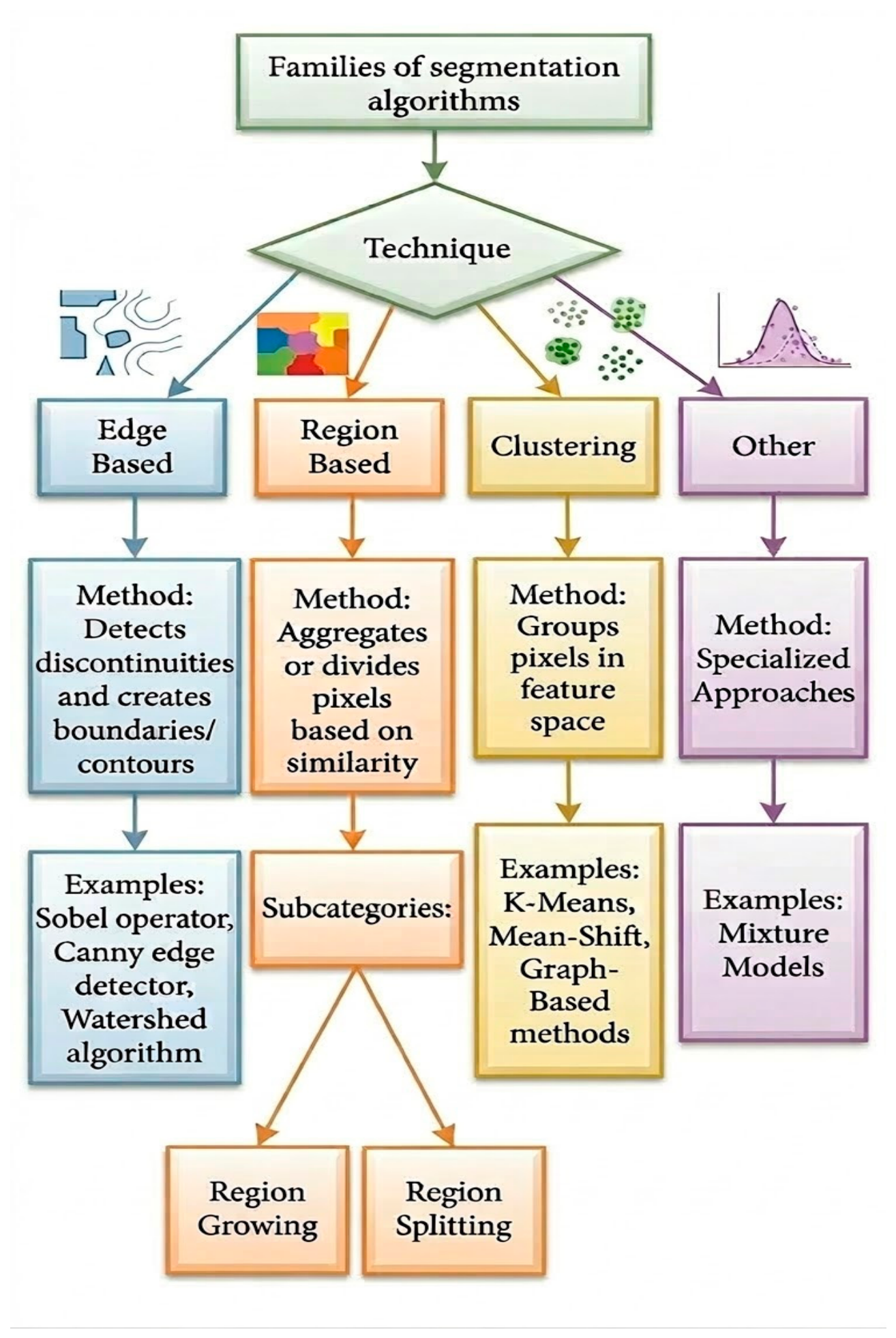
Figure 3.
Illustrative examples of the operation of the four families of image segmentation algorithms.
Figure 3.
Illustrative examples of the operation of the four families of image segmentation algorithms.
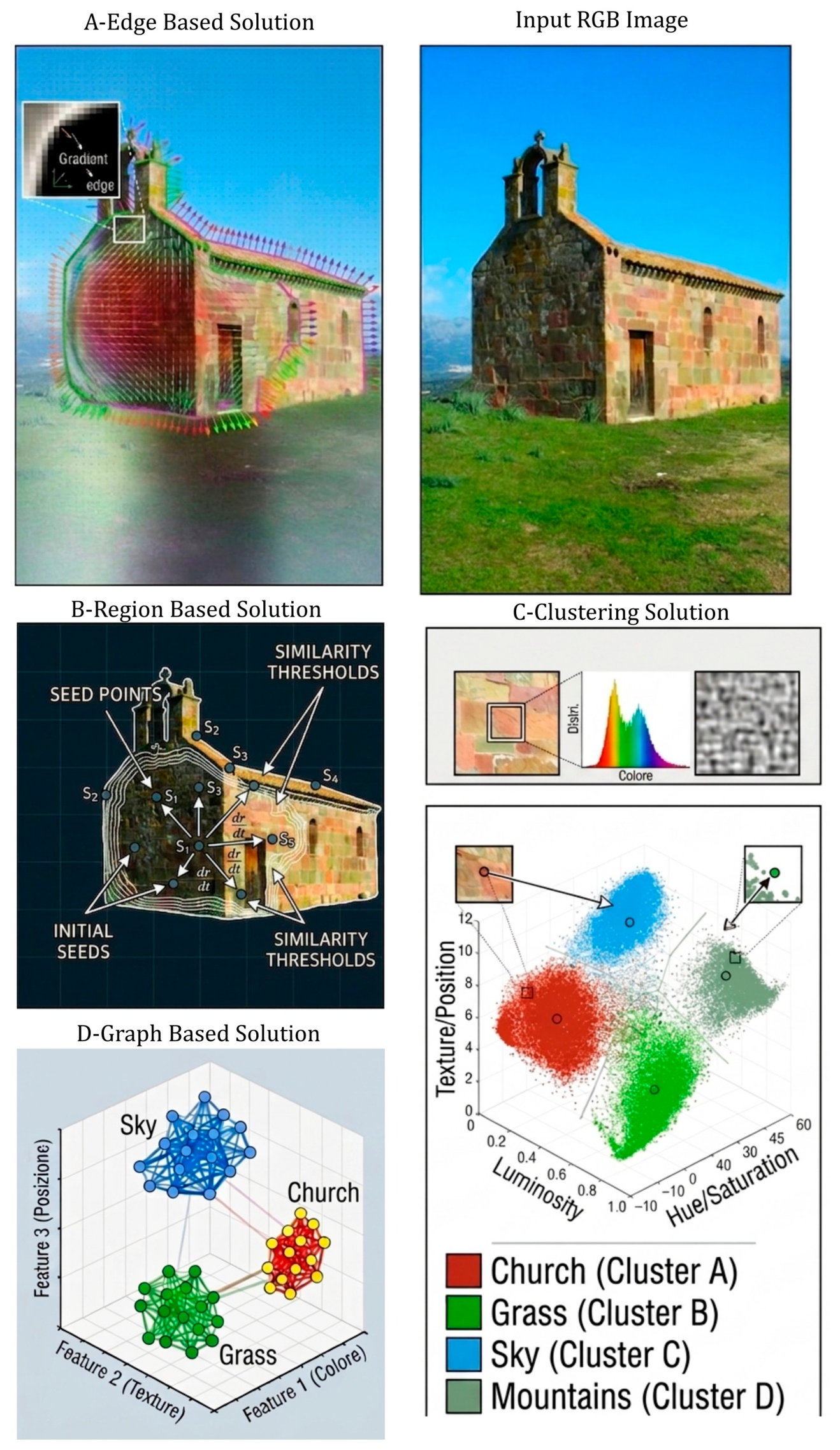
Figure 4.
Illustrative example of the segmentation process obtained through variational method.
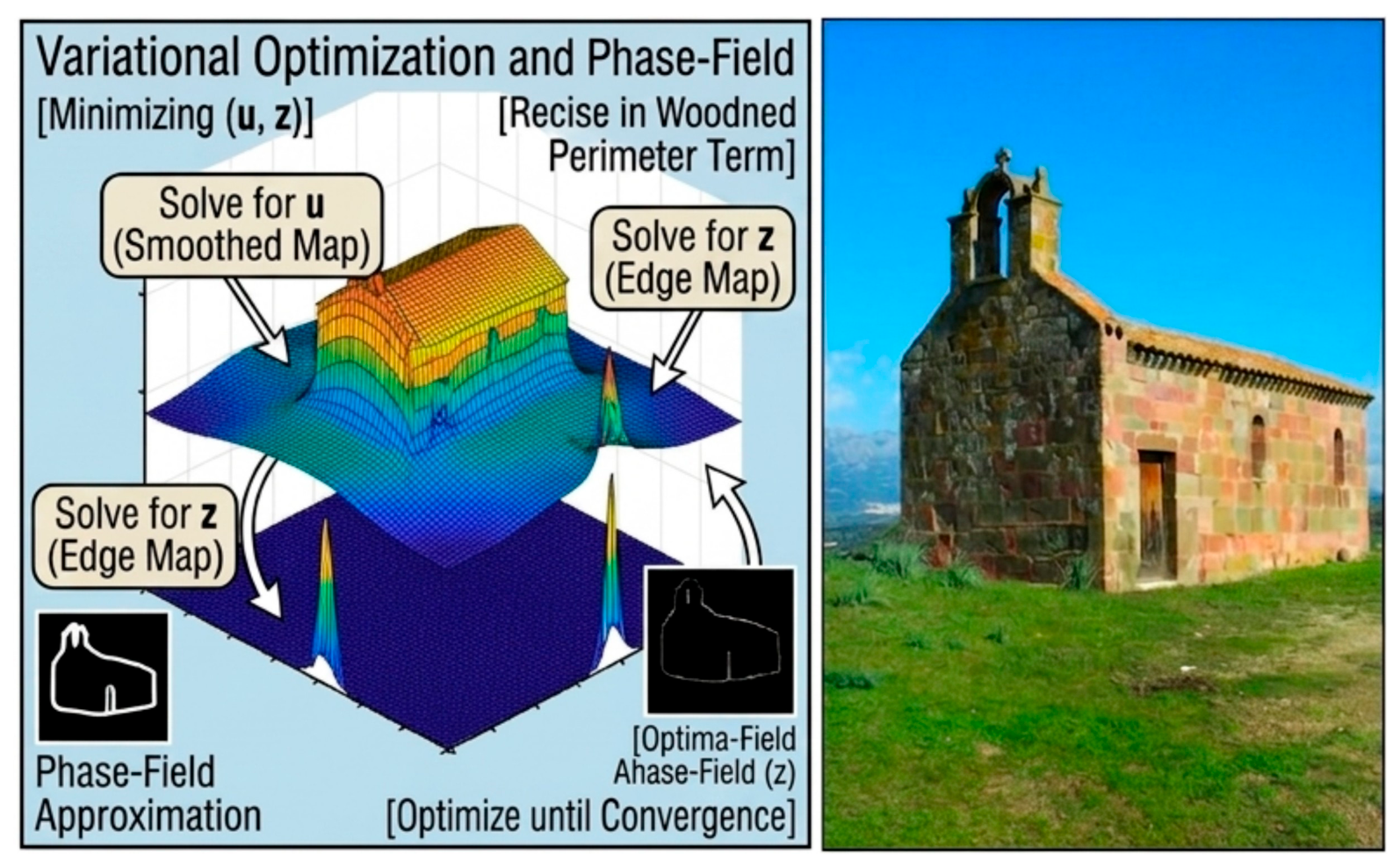
Figure 5.
Step 1 output for a representative rural scene featuring an agricultural holding and road infrastructure. From top-left clockwise: original RGB image, grayscale rendering, binary classification mask overlaid in red (Otsu threshold = 0.412, η = 0.795), and RF probability map P(object).
Figure 5.
Step 1 output for a representative rural scene featuring an agricultural holding and road infrastructure. From top-left clockwise: original RGB image, grayscale rendering, binary classification mask overlaid in red (Otsu threshold = 0.412, η = 0.795), and RF probability map P(object).
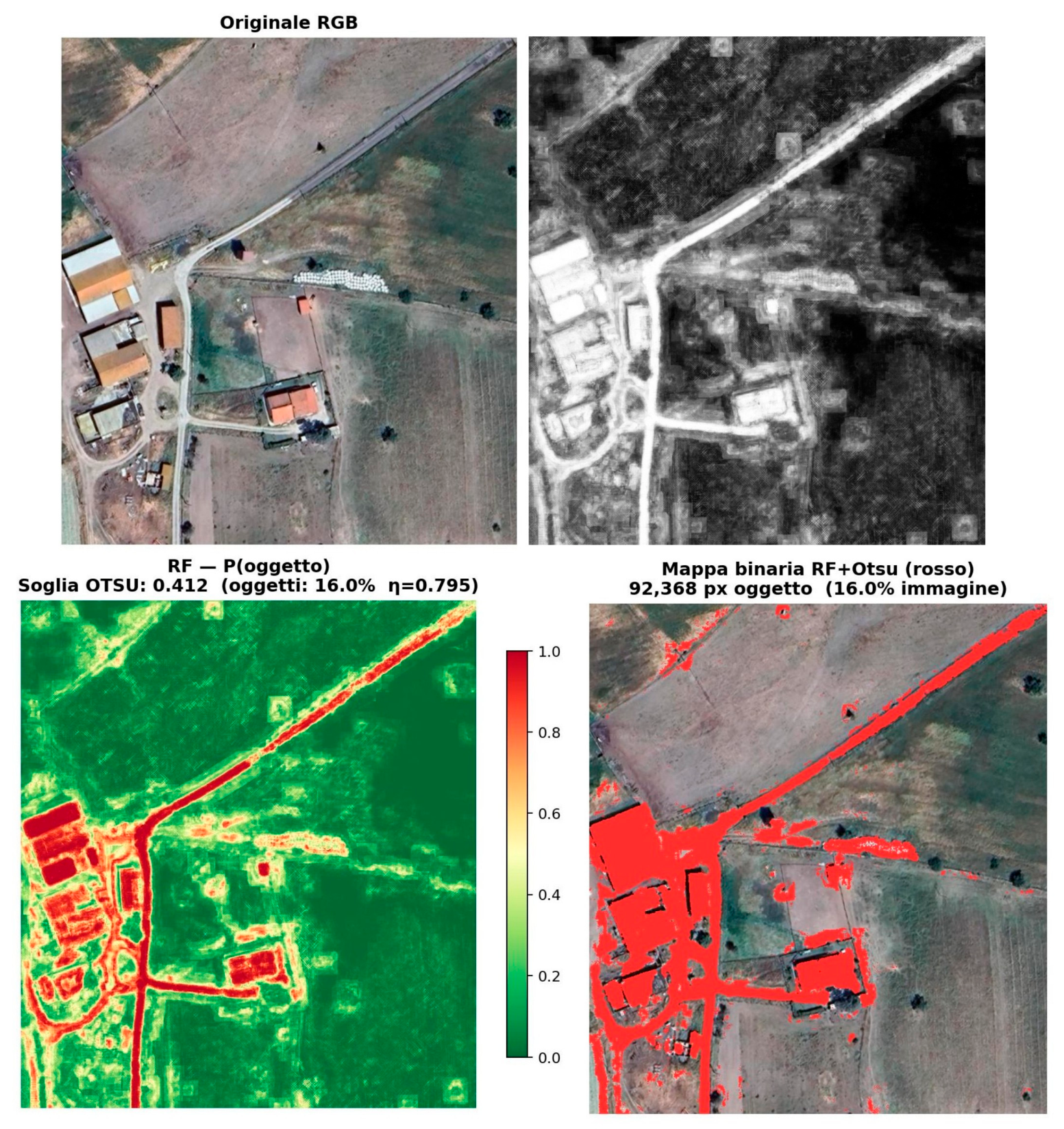
Figure 6.
Ambrosio-Tortorelli Execution Algorithm.
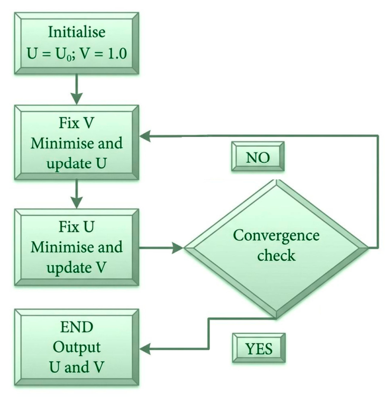
Figure 8.
Step 4 intermediate outputs for the same scene. Left: strong edge pixels extracted from the AT edge map (GMM threshold 1−v ≥ 0.1534, 9,586 pixels) overlaid in red on the original RGB image. Right: 243 candidate object centres identified by KDE (cyan markers, adaptive bandwidth = 3.0 px), which serve as point prompts for SAM in the subsequent segmentation step.
Figure 8.
Step 4 intermediate outputs for the same scene. Left: strong edge pixels extracted from the AT edge map (GMM threshold 1−v ≥ 0.1534, 9,586 pixels) overlaid in red on the original RGB image. Right: 243 candidate object centres identified by KDE (cyan markers, adaptive bandwidth = 3.0 px), which serve as point prompts for SAM in the subsequent segmentation step.
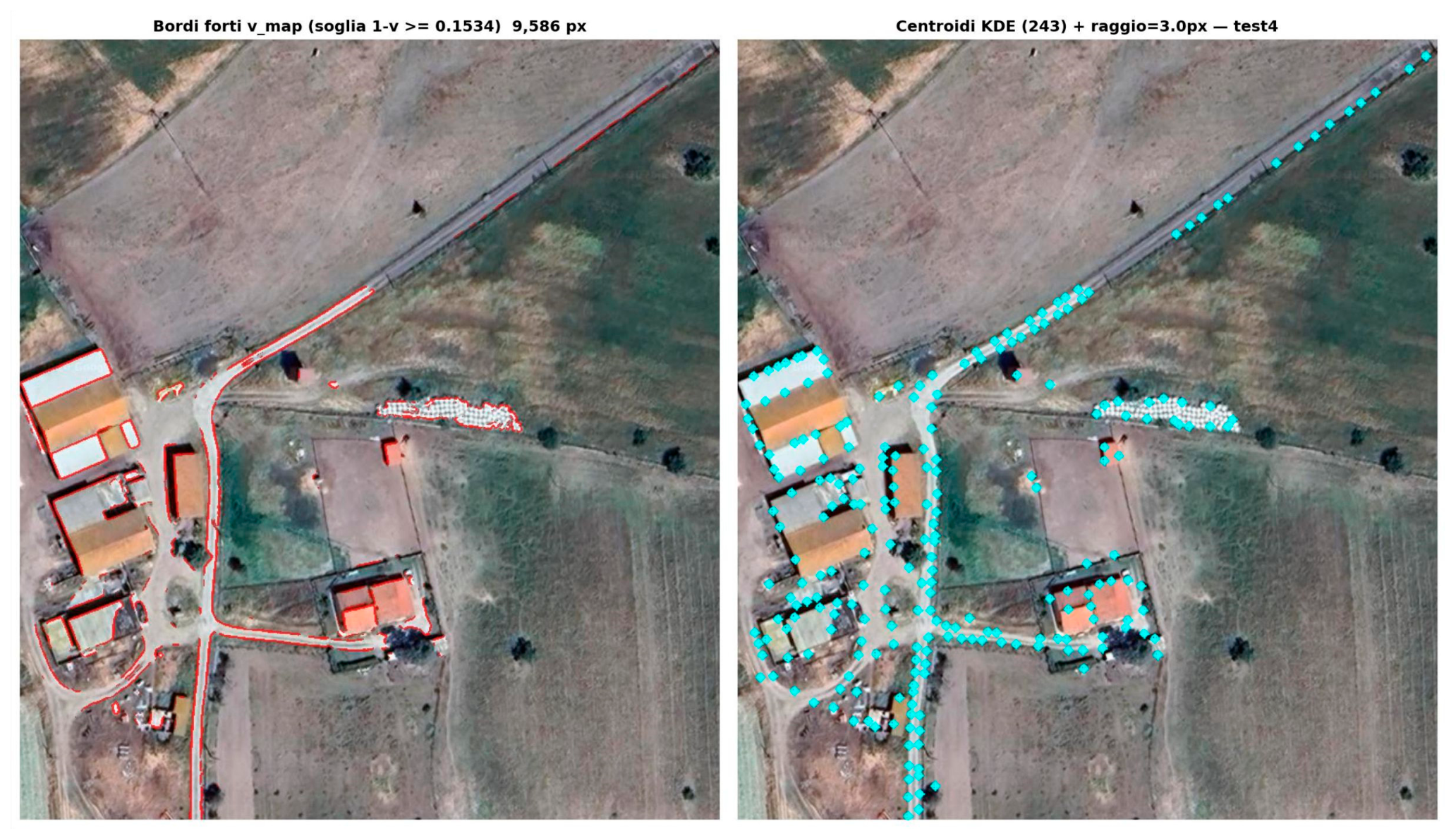
Figure 9.
Step 4 final output for the same scene: 186 SAM masks retained after GMM-based RF probability filtering, each rendered in a distinct semi-transparent colour. Individual building footprints, road segments, and ancillary structures are delineated as separate objects against the unmasked agricultural background.
Figure 9.
Step 4 final output for the same scene: 186 SAM masks retained after GMM-based RF probability filtering, each rendered in a distinct semi-transparent colour. Individual building footprints, road segments, and ancillary structures are delineated as separate objects against the unmasked agricultural background.
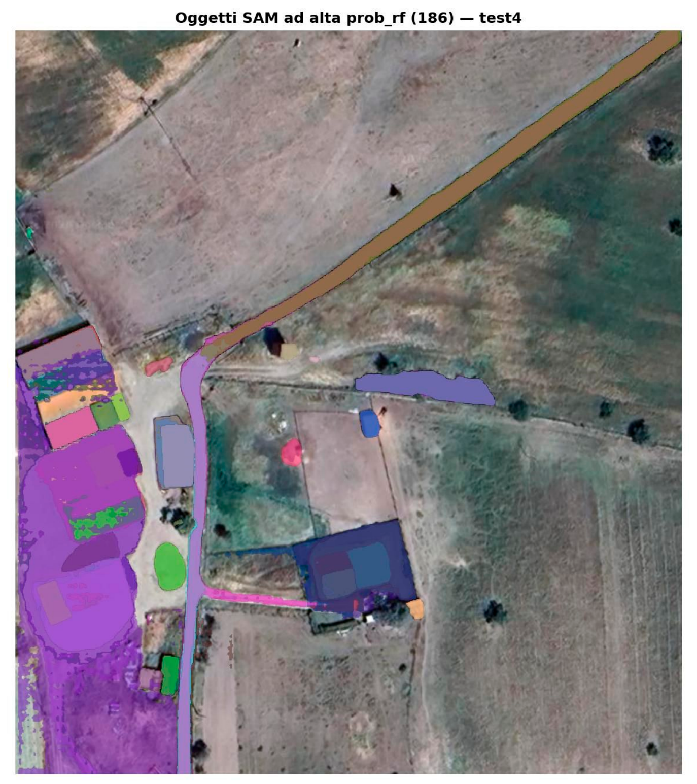
Figure 7.
Step 2/3 output for the same scene. Left: modulated image. Right: AT edge map (1−v), where brighter values indicate stronger discontinuities (v min = 0.175); the agricultural background is effectively suppressed while building footprints and road edges are sharply delineated.
Figure 7.
Step 2/3 output for the same scene. Left: modulated image. Right: AT edge map (1−v), where brighter values indicate stronger discontinuities (v min = 0.175); the agricultural background is effectively suppressed while building footprints and road edges are sharply delineated.
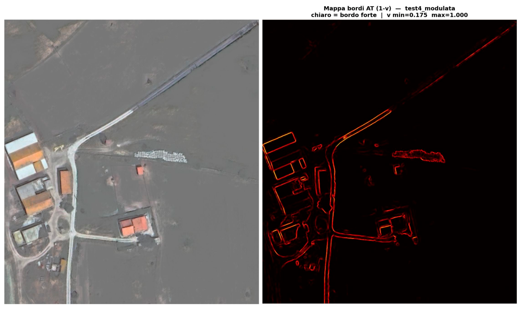
Figure 10.
Illustrative example of the interpretive difficulty faced by classification algorithms due to the inevitable seasonal cycle.
Figure 10.
Illustrative example of the interpretive difficulty faced by classification algorithms due to the inevitable seasonal cycle.
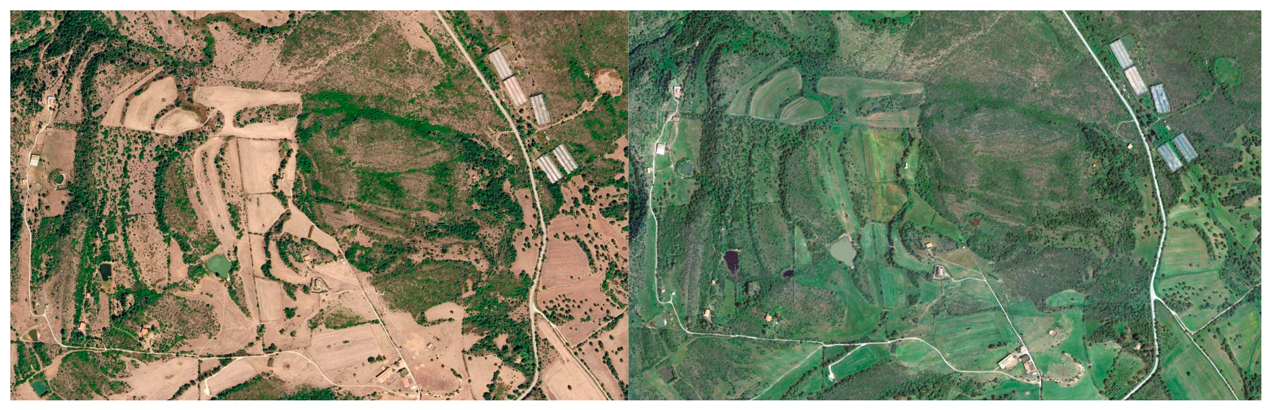
Figure 11.
Some of the selected test areas.
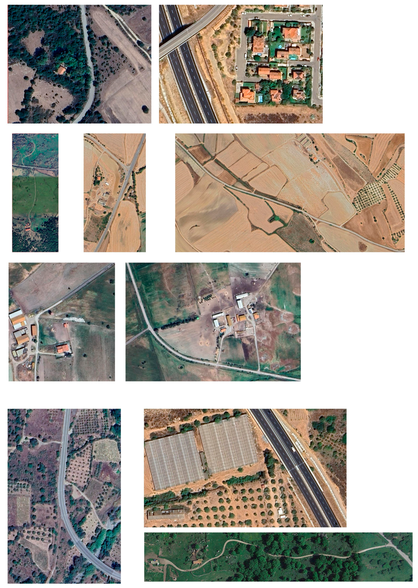
Figure 12.
Step 1 results for the five low-difficulty test scenes (test1, test4, test5, test6, test9). For each scene: original RGB image (left), RF probability map P(object) (centre), and binary classification mask overlaid in red (right). All scenes exhibit high Otsu thresholds and strongly bimodal distributions, reflecting clear radiometric separability between infrastructure and agricultural background.
Figure 12.
Step 1 results for the five low-difficulty test scenes (test1, test4, test5, test6, test9). For each scene: original RGB image (left), RF probability map P(object) (centre), and binary classification mask overlaid in red (right). All scenes exhibit high Otsu thresholds and strongly bimodal distributions, reflecting clear radiometric separability between infrastructure and agricultural background.
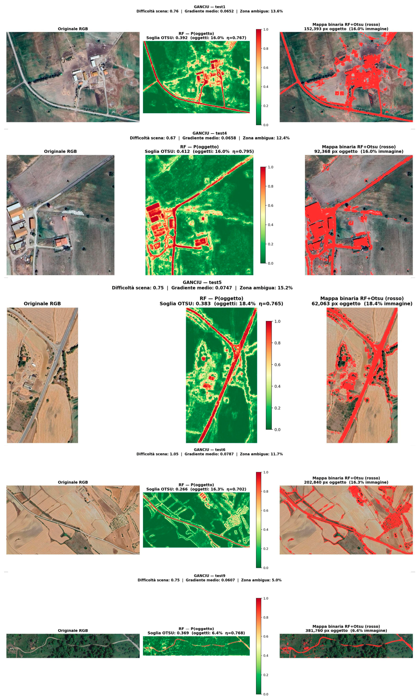
Figure 13.
Step 1 results for the four intermediate-difficulty test scenes (test2, test3, test13, test14). For each scene: original RGB image (left), RF probability map P(object) (centre), and binary classification mask overlaid in red (right). Compared to the low-difficulty group, lower Otsu thresholds and wider ambiguous zones reflect the increased spectral overlap between infrastructure and background, particularly in scenes with dense vegetation and greenhouse structures.
Figure 13.
Step 1 results for the four intermediate-difficulty test scenes (test2, test3, test13, test14). For each scene: original RGB image (left), RF probability map P(object) (centre), and binary classification mask overlaid in red (right). Compared to the low-difficulty group, lower Otsu thresholds and wider ambiguous zones reflect the increased spectral overlap between infrastructure and background, particularly in scenes with dense vegetation and greenhouse structures.
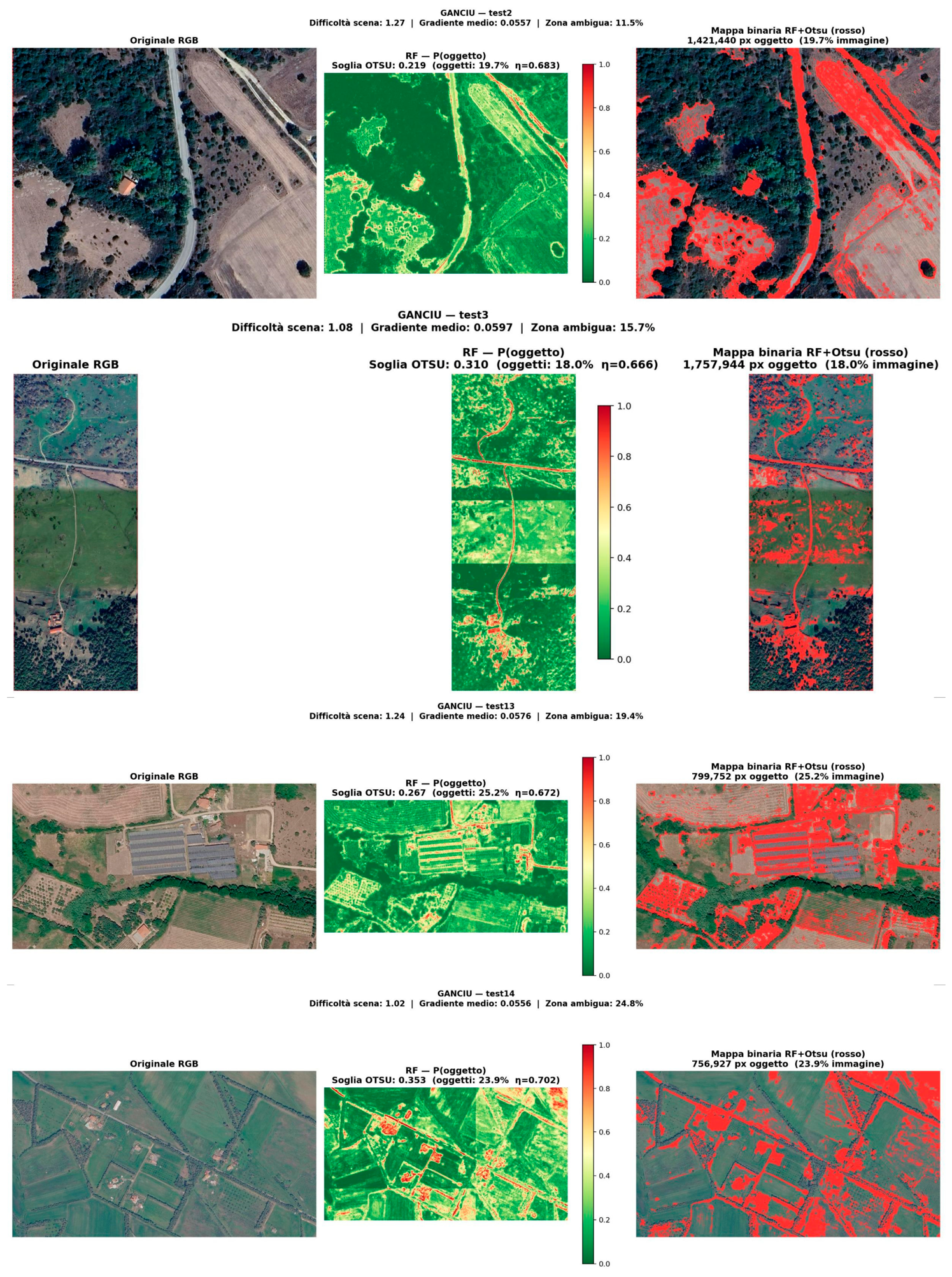
Figure 14.
Step 1 results for the two high-difficulty test scenes (test7, test8). For each scene: original RGB image (left), RF probability map P(object) (centre), and binary classification mask overlaid in red (right). Both scenes exhibit ambiguous zones exceeding 46%, with probability maps dominated by intermediate values reflecting the severe spectral overlap between built surfaces, road infrastructure, greenhouse structures, and surrounding vegetation.
Figure 14.
Step 1 results for the two high-difficulty test scenes (test7, test8). For each scene: original RGB image (left), RF probability map P(object) (centre), and binary classification mask overlaid in red (right). Both scenes exhibit ambiguous zones exceeding 46%, with probability maps dominated by intermediate values reflecting the severe spectral overlap between built surfaces, road infrastructure, greenhouse structures, and surrounding vegetation.
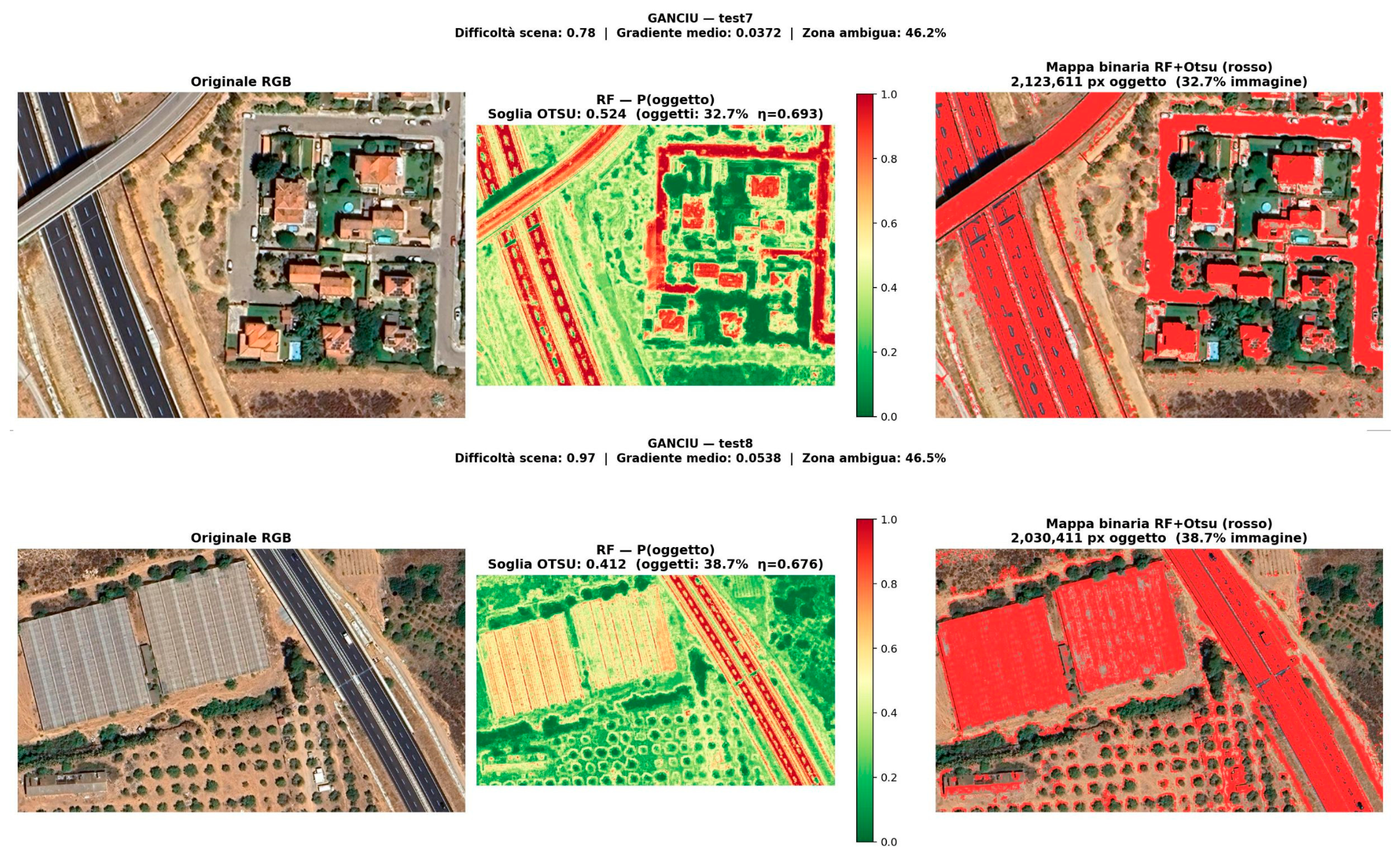
Figure 15.
Step 1 results for the three agriculturally dominated test scenes (test10, test11, test12). For each scene: original RGB image (left), RF probability map P(object) (centre), and binary classification mask overlaid in red (right). The probability maps reveal the primary failure mode of the current model: anomalously high probabilities assigned to intensive crop surfaces — olive groves, row crops, and dense woodland edges — in the absence of significant built infrastructure.
Figure 15.
Step 1 results for the three agriculturally dominated test scenes (test10, test11, test12). For each scene: original RGB image (left), RF probability map P(object) (centre), and binary classification mask overlaid in red (right). The probability maps reveal the primary failure mode of the current model: anomalously high probabilities assigned to intensive crop surfaces — olive groves, row crops, and dense woodland edges — in the absence of significant built infrastructure.
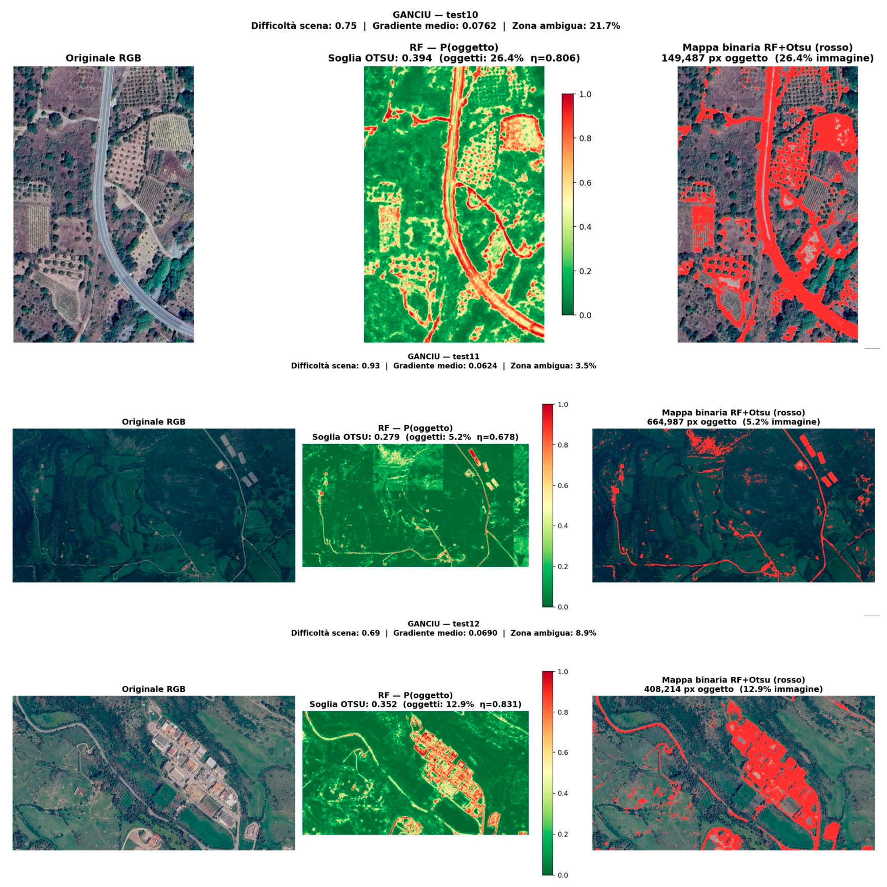
Figure 16.
Step 3 AT edge maps (1−v) for four representative test scenes (test8, test1, test4, test10). Brighter values indicate stronger discontinuities. The contrast between scenes is instructive: test8 and test4 produce sharp, geometrically well-defined contours around building footprints and road edges, while test10 reveals the failure mode of the modulation step, with diffuse edge responses distributed across intensive crop surfaces rather than concentrated on infrastructure boundaries.
Figure 16.
Step 3 AT edge maps (1−v) for four representative test scenes (test8, test1, test4, test10). Brighter values indicate stronger discontinuities. The contrast between scenes is instructive: test8 and test4 produce sharp, geometrically well-defined contours around building footprints and road edges, while test10 reveals the failure mode of the modulation step, with diffuse edge responses distributed across intensive crop surfaces rather than concentrated on infrastructure boundaries.
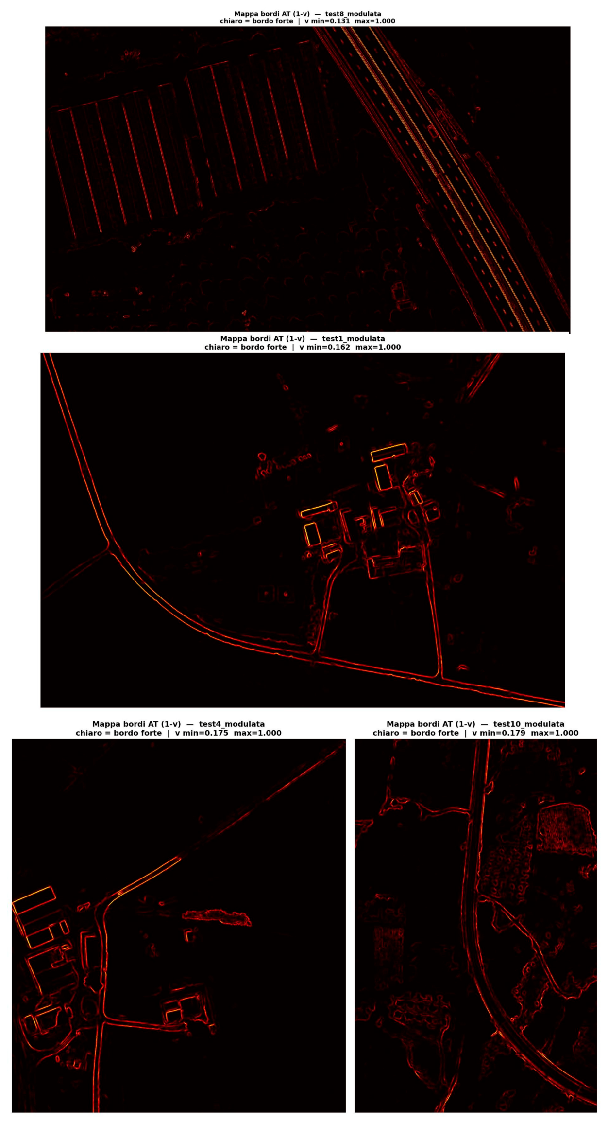
Figure 17.
Step 4 final output for two contrasting scenes. Top (test1): 222 SAM masks retained after RF filtering, showing precise delineation of individual building footprints, warehouses, and road segments in a scene with clear radiometric contrast. Bottom (test14): 167 masks retained despite a difficulty index of 1.02, demonstrating the pipeline's recovery capacity in a spectrally ambiguous scene dominated by agricultural parcels and scattered rural buildings.
Figure 17.
Step 4 final output for two contrasting scenes. Top (test1): 222 SAM masks retained after RF filtering, showing precise delineation of individual building footprints, warehouses, and road segments in a scene with clear radiometric contrast. Bottom (test14): 167 masks retained despite a difficulty index of 1.02, demonstrating the pipeline's recovery capacity in a spectrally ambiguous scene dominated by agricultural parcels and scattered rural buildings.
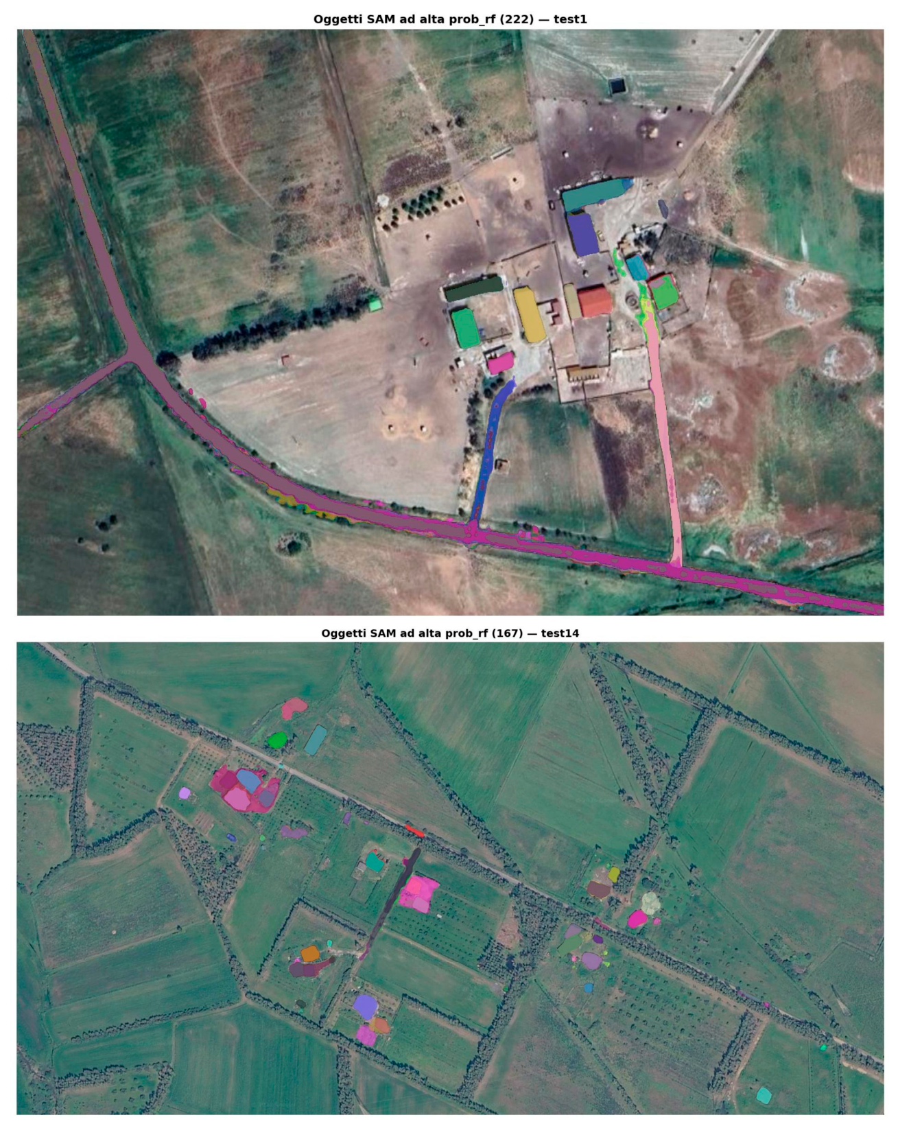
Figure 18.
Step 4 final output for the two agriculturally dominated failure cases. Top (test11): 428 masks retained out of 608, predominantly false positives scattered across forested and grassland surfaces in the absence of genuine infrastructure. Bottom (test12): 754 masks retained, with large contiguous segments covering cultivated parcels rather than built structures, illustrating the pipeline's most critical failure mode when the RF training set lacks sufficient representation of intensive agricultural backgrounds.
Figure 18.
Step 4 final output for the two agriculturally dominated failure cases. Top (test11): 428 masks retained out of 608, predominantly false positives scattered across forested and grassland surfaces in the absence of genuine infrastructure. Bottom (test12): 754 masks retained, with large contiguous segments covering cultivated parcels rather than built structures, illustrating the pipeline's most critical failure mode when the RF training set lacks sufficient representation of intensive agricultural backgrounds.
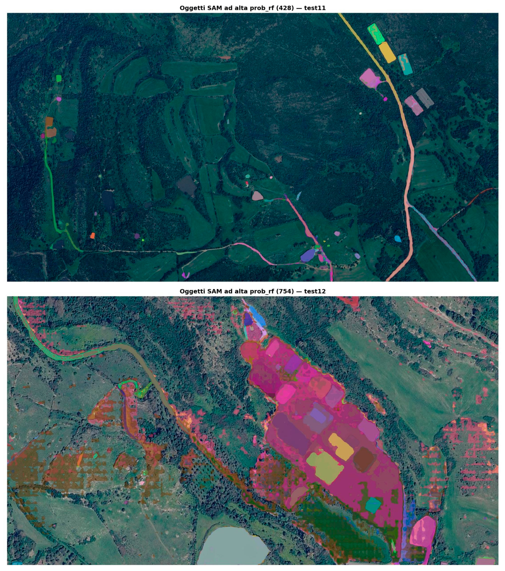

Table 1.
A classification of algorithms according to Supervised versus Unsupervised and Parametric versus Non-parametric methodologies.
Table 1.
A classification of algorithms according to Supervised versus Unsupervised and Parametric versus Non-parametric methodologies.
| Parametric | Non-parametric | |
| Supervised | Maximum Likelihood Classifier (MLC); Regressione Logistica |
Random Forest (RF) Support Vector Machine (SVM) K-Nearest Neighbours (KNN) Neural Networks (ANN) |
| Unsupervised | Gaussian Mixture Models (GMM) | K-Means ISODATA DBSCAN Hierarchical Clustering |
Disclaimer/Publisher’s Note: The statements, opinions and data contained in all publications are solely those of the individual author(s) and contributor(s) and not of MDPI and/or the editor(s). MDPI and/or the editor(s) disclaim responsibility for any injury to people or property resulting from any ideas, methods, instructions or products referred to in the content. |
© 2026 by the authors. Licensee MDPI, Basel, Switzerland. This article is an open access article distributed under the terms and conditions of the Creative Commons Attribution (CC BY) license.
Copyright: This open access article is published under a Creative Commons CC BY 4.0 license, which permit the free download, distribution, and reuse, provided that the author and preprint are cited in any reuse.


