

Submitted:
07 July 2026
Posted:
09 July 2026
You are already at the latest version
Abstract
Accurate stroke prediction is vital for early intervention, yet most high-performing AI/ML models remain “black boxes” with little intrinsic interpretability. Bayesian net-works (BNs) are probabilistic graphical models that balance predictive performance with interpretable, auditable reasoning. We assessed whether optimizing data preprocessing could enhance BNs diagnostic performance on a highly imbalanced stroke dataset. Using a 2×2×2 factorial design, we compared eight configurations varying three choices: dis-cretized versus continuous (conditional Gaussian) topology, median versus multiple imputation by chained equations (MICE), and no balancing versus synthetic over-sampling (SMOTE). Preserving continuous variables significantly improved discrimina-tion over discretization (AUC 0.812 vs 0.718; p = 0.011), an advantage that persisted across 30 stratified resamples (paired p < 0.001); the hybrid BN matched XGBoost (0.822) and logistic regression (0.819). MICE gave no advantage over median substitution (p = 0.708), and SMOTE did not improve performance while tripling the Brier score, indicating posterior miscalibration. The optimal BN remained interpretable and could simulate illustrative absolute risk reductions (e.g., 43.18% to 31.55% under modelled glycemic control). Continuous BNs offer an interpretable, well-calibrated, and robust framework for clinical decision support, warranting prospective validation in real-world settings.
Keywords:
Bayesian networks
; explainable AI (XAI)
; stroke risk prediction
; machine learning
1. Introduction
Stroke is a leading cause of death and disability in Canada and worldwide [1]. It has been estimated that up to 80% of strokes are preventable through timely identification and targeted screening of risk factors, including hypertension, smoking, diabetes and other vascular risks [2]. In the United States, stroke mortality has declined by more than 70% over the past 50 years through advancements in prevention, acute care, and secondary risk reduction [2].
However, substantial disparities persist globally, which drives uneven access to screening, timely care, and health education [3]. For example, approximately 40% of patients presenting to emergency departments with acute stroke are unaware of warning signs and etiological risk factors [4].
The shift toward precision medicine has fundamentally reshaped the paradigms of disease risk stratification, moving away from “one-size-fits-all” screening toward data-driven, personalized risk assessment [5]. As established by Steyerberg et al. [6], the methodology of clinical prediction has expanded significantly beyond the foundational use of logistic regression and linear classifiers. While these models are the gold standard for transparency, the increasing availability of high-resolution electronic health records (EHR) has demanded more flexible algorithmic approaches. This evolution spans from rule-based expert systems and decision trees to probabilistic frameworks and sophisticated deep learning models [6,7,8]. While the increasing complexity of algorithmic models captures the intricate interplay among disease risk factors, it obscures the transparency of the underlying mathematical models. The schematic architecture of these models is shown in Supplementary material, Figure S1.
The simpler condition-based model, rule-based learning, relies on predefined sets of rules and represents a highly transparent approach. This transparency and logic of explicit conditions inspired the automated, hierarchical data splitting used in decision trees [9]. Similarly, K-nearest neighbors (KNN) and support vector machines (SVMs) solve nonlinearity by classifying patient risk mathematically via spatial distance and geometric hyperplanes [10,11]. Generalized additive models (GAMs) provide flexibility by isolating continuous variables (e.g., blood pressure) into standalone risk curves [12], whereas Bayesian networks use directed acyclic graphs to calculate explicit conditional probabilities between interdependent risk factors [6]. At the upper end of the model’s structural complexity, Ensembles (e.g., Random Forests and XGBoost) aggregate hundreds of individual models to generate a weighted consensus, and deep learning networks process high-dimensional variables through layers of hidden computational nodes [13].
Machine learning models, particularly neural networks and XGBoost, often achieve high predictive performance [14]. However, these models are frequently classified as “black-box” models, as the underlying reasoning of diagnostic decisions remains obscured from human interpretation [15,16]. This lack of transparency presents a critical barrier in high-stakes medical settings, where both healthcare providers and patients are often unable to discern the underlying biological rationale required to confidently trust and act upon the algorithmic output.
Conversely, traditional statistical approaches such as logistic and linear regression remain cornerstone tools in clinical risk prediction [17]. Within the formal taxonomy of explainable artificial intelligence (XAI), these models are classified as “transparent” [18], “white-box” [19] or “glass-box” [20] models, which characterize algorithms by their intrinsic interpretability.
Interpretability is formally defined as the degree to which a human can consistently predict the model’s result and comprehend the underlying cause of a decision [21]. It is the extent to which the internal mechanics of a model make sense to a human observer without requiring supplementary, post hoc explanations.
Arrieta et al. [18] characterize transparency through 3 hierarchical dimensions as listed below:
- Simulatability: A clinician can mentally or manually calculate a patient's stroke risk via a simple scoring system (e.g., adding points for age and hypertension).
- Decomposability: A physician can isolate and understand the specific weight (coefficient) assigned to a single variable, such as observing how a 10 mmHg increase in blood pressure explicitly shifts the risk output.
- Algorithmic transparency: The mathematical guarantee that a model will converge on a unique, optimal solution for a patient's risk profile, driven by a visible optimization process such as maximum likelihood estimation.
Expanding upon structural transparency, Doshi-Velez and Kim [22] propose a rigorous taxonomy for evaluating interpretability through three distinct task-driven categories.
- Application-grounded evaluations: This involves conducting experiments with domain experts within the context of real-world tasks, such as a neurologist evaluating the model’s output while diagnosing acute stroke patients in the emergency department.
- Human-grounded evaluations: Layperson or nonspecialist clinicians are tasked with identifying the most weighted risk factor from visual dashboards or charts.
- Functionally grounded evaluations: Researchers benchmarking a highly complex model (like a neural network) against mathematically transparent models (like a decision tree) without requiring live human experiments.
While these transparent architectures ensure clinical accountability, their intrinsic interpretability frequently comes at the expense of predictive accuracy [23]. Although these models may perform optimally within highly structured and well-defined datasets, they lack the mathematical flexibility required to map the widespread, nonlinear dependencies inherent in real-world clinical data [18]. Consequently, developing targeted diagnostic tools requires navigating a trade-off between maximizing performance and preserving structural transparency, as illustrated in Supplementary material, Figure S2.
The trade-off exhibits a Pareto frontier, where models inherently sacrifice mathematical visibility to achieve higher dimensionality. Arrieta et al. outlined two primary research trajectories for modern clinical diagnostics [18]. The first involves applying post hoc explainability techniques such as Shapley additive explanation (SHAP) [24] or local interpretable model-agnostic explanations (LIME) [25]. This is to estimate feature importance and approximate the logic of highly accurate, opaque models. Alternatively, researchers are developing hybrid modeling approaches that enhance the performance of interpretable models via advanced preprocessing techniques and hybrid models.
Lolak et al. [26] compared the performance and interpretability of logistic regression, Cox proportional hazard, Bayesian network, tree-augmented naïve Bayes (TAN), extreme gradient boosting (XGBoost), and explainable boosting machine (EBM) methods for predicting stroke risk. They included a retrospective cohort of 275,247 high-risk patients with discretized risk factors, including demographic, cardiovascular, and metabolic variables and medication use. Among these patients, 9659 (3.5%) experienced strokes. Multiple imputation by chained equation (MICE) was implemented for missing risk factors. The C statistics of XGBoost, EBM, TAN, logistic regression and the Bayesian network were 0.89, 0.87, 0.83, 0.80 and 0.80, respectively. However, XGBoost needs post hoc analysis to improve explainability. On the other hand, the explainability of these models has been less explored.
The optimal diagnostic model is dictated by the dataset’s architecture and the need for interpretability [15], as the “No Free Lunch” theorem establishes that no single algorithmic approach is universally superior across the entire dataset [27]. While deep learning excels at extracting features from massive, unstructured datasets, tree-based ensembles such as XGBoost frequently outperform neural networks on structured, tabular electronic health record (EHR) data [13,28]. Conversely, parsimonious algorithms such as logistic regression and Bayesian networks offer superior mathematical interpretability in cohorts characterized by limited sample sizes or significant data missingness [6]. Furthermore, selecting clinically relevant nonredundant features via effective feature selection not only mitigates the “curse of dimensionality” but also ensures that the resulting diagnostic model remains both mathematically sound and biologically plausible [6].
To bridge the gap between predictive performance and model interpretability, Bayesian networks (BNs) present a parsimonious alternative. On the accuracy‒interpretability continuum, BNs occupy a strategic intermediate position that bridges simpler transparent models and high-performing opaque architectures. The mathematical foundation of a Bayesian network (BN) is Baye’s theorem, which provides a rigorous framework for updating the probability of a clinical hypothesis (, such as a stroke diagnosis) on the basis of observed evidence (, such as specific patient risk factors):
The term represents the posterior probability, which is the probability of the hypothesis given the evidence. In a clinical context, this allows for dynamic risk assessment where the prior probability , which is based on population prevalence, is redefined into a personalized risk score as individual patient data are integrated.
A Bayesian network extends this principle into a probabilistic graphical model that represents the joint probability distribution of a complex set of clinical variables. As illustrated in the sequential architecture of Figure 1, the model decomposes high-dimensional data into a product of local conditional distributions via the following theorem:
The conditional probability table (CPT) serves as the primary parameterization of the network. Each CPT quantifies the probabilistic relationship between a "child" node and its "parent" nodes by explicitly listing the probability of every possible child state given all combinations of parent states. For example, a CPT for the node "Stroke" calculates specific risk probabilities on the basis of discrete parent states such as "Old Age" and "High Glucose". This modular structure ensures that the model remains decomposable, as individual tables can be isolated and audited by clinicians to verify that the algorithmic logic remains biologically plausible and aligned with clinical domain expertise.
Bayesian networks have been implemented in disease diagnosis and risk prediction, including for cardiovascular disease [29], atrial fibrillation relapse [30], and ALS diagnosis [31]. Suo et al. [32] developed a BN-based model using EHR data from 169,692 patients in Chinese hospitals to predict 3-year CHD risk. A weighted survival Bayesian network was developed by combining inverse probability censoring weights and a Cox model using demographic, laboratory and medical history variables as risk factors. The model achieved an AUC of 0.80 despite extensive missing data and imbalanced datasets.
Similarly, Park et al. [33] applied a BN to predict 3-month functional outcomes (mRS) and 1-year mortality in 2,432 ischemic stroke patients using 74 features (risk factors), including baseline NIHSS scores and age, attaining an AUC of 0.89 for 3-month functional outcomes and 0.89 for 1-year mortality. They also developed a Yonsei outcome inference system via their trained model.
Lolak et al. [26] demonstrated the utility of BNs in a retrospective cohort of 275,247 high-risk patients compared with other machine learning models. Although XGBoost achieved a superior C statistic of 0.89, the BN model demonstrated a competitive value of 0.80 while maintaining intrinsic interpretability. with numerous features.
Despite their utility in a large cohort and ability to capture many clinical features, BNs often lag in discriminatory performance. This predictive gap arises from inappropriate handling of missing data, inadequate preprocessing techniques and imbalanced targeted classes.
To address this limitation without sacrificing the intrinsic transparency of the BN model, our research aligns with the objective of increasing the predictive capability of BNs. By implementing rigorous data preprocessing techniques and utilizing a hybrid modeling structure to accommodate continuous variables, this study aims to close the accuracy gap.
We present a rigorous, eight-arm methodological ablation study evaluating the predictive architecture of Bayesian networks. We systematically isolate the effects of network topology (purely discretized vs. hybrid continuous nodes), imputation strategies (baseline median imputation vs. multiple imputation by chained equations [MICE]), and class balancing (unadjusted vs. synthetic minority oversampling technique [SMOTE]).
By isolating the effect of each methodological variation, the following hypothesis has been constructed:
| Focus Area | Null Hypothesis (H0) | Alternate Hypothesis (H1) |
| 1. Topology | Hybrid continuous topology does not significantly change predictive performance vs. pure discretization. | Hybrid continuous topology significantly changes predictive performance vs. pure discretization. |
| 2. Imputation | MICE does not significantly improve performance metrics vs. baseline median imputation. | MICE significantly improves performance metrics vs. baseline median imputation. |
| 3. Balancing | SMOTE does not significantly increase minority class sensitivity vs. unadjusted distributions. | SMOTE significantly increases minority class sensitivity vs. unadjusted distributions. |
| 4. Synergy | The integration of continuous topology, MICE, and SMOTE does not significantly improve overall capacity vs. baseline. | The integration of continuous topology, MICE, and SMOTE significantly improves overall capacity vs. baseline. |
2. Materials and Methods
Ethical approval and informed consent were not required for this study. We used an open-source Stroke prediction dataset, which is available at Kaggle [34]. The dataset has been widely adopted in machine learning research, with approximately 290,000 downloads, and is used in 103 research articles [35].
2.1. Overview of the Dataset
The dataset consists of 10 features along with the diagnosis of stroke. The dataset is highly imbalanced, with 4861 nonstroke patients and 249 stroke patients with a stroke incidence of 4.9%. The summary of the feature is shown in Supplementary material, Table S1.
The dataset features incorporate continuous, binary and categorical values. These features are broadly categorized in the following aspects:
- Sociodemographics: age, sex, residence type, marital status and occupation
- Medical history: Hypertension and heart disease
- Physiological measurements: BMI (body‒mass index) and average glucose level
- Lifestyle factor: Smoking status
Reshetnyak et al. demonstrated that cumulative sociodemographic factors serve as significant, independent predictors of incident stroke [36]. Similarly, the landmark INTERSTROKE study in the Lancet revealed that risk factors such as hypertension, cardiac history, BMI, glucose levels, and smoking status collectively account for approximately 90% of the population-attributable risk for stroke [37].
Continuous variables need to be converted to categorical variables for the Bayesian network. Age was categorized on the basis of the WHO’s standard age group (differences of 5 and 85+) [38]. Similarly, body mass index (BMI) has also been categorized on the basis of the WHO [39]: underweight (less than 18.4 kg/m2), normal weight (18.5 to 24.9 kg/m2), overweight (25 to 29.9 kg/m2) and obese (greater than 29.9 kg/m2). Diabetes was classified as present if the average glucose was ≥126 mg/dL, prediabetes if 100–125 mg/dL, and normal if <100 mg/dL [40]. This glucose-only approach ensures consistency in aggregated data while acknowledging limitations such as ignoring timing, symptoms, A1C, medications, and comorbidities that influence accurate diagnosis.
Alternately, we maintain these variables in their continuous form by employing a hybrid Bayesian network (HBN) structure [41]. To implement this hybrid approach, the following steps were taken:
- Age, BMI and average glucose were preserved as exact numeric values.
- The conditional distribution of continuous nodes was specified by a Gaussian function via conditional linear Gaussian distributions.
- We utilized structure and parameter learning algorithms explicitly designed for mixed-data networks to estimate outcomes accurately.
2.2. Study Design
This study employs a 2x2x2 factorial design to evaluate the impact of different data preparation techniques on model performance. Figure 1 illustrates the overall methodological framework, distinguishing between standard pipeline procedures and experimental variables. The baseline methodology (Model M1) establishes a fixed processing pipeline that is applied uniformly across all the models. To prevent data leakage, a standard training-validation test (60-20-20) split is executed prior to any data manipulation. Following the split, preprocessing choices are applied: median missing value imputation, feature discretization, and no class balancing.
2.3. Study Arms
To evaluate potential improvements over the baseline, three experimental variations were introduced at key methodological decision points (denoted by dashed lines in Figure 1):
- Imputation: Median vs. MICE
- Feature type: Discretized vs. Continuous
- Training Set Balancing: None vs. SMOTE
Based on the permutations of these three variables, the data were processed through eight distinct analytical study arms (Models M1 through M8), as detailed in Table 1. This configuration effectively isolates the individual and combined effects of MICE, continuous features, and SMOTE, allowing for a comprehensive comparison of how each preprocessing variation impacts overall predictive accuracy.
2.4. Structure Learning
The structure of the Bayesian networks (BNs) was learned via the hill-climbing (HC) heuristic search algorithm. To reduce computational overhead and ensure clinical validity, we implemented whitelisting and blacklisting techniques. The strongly associated nodes were whitelisted, and biologically impossible edges (such as blood pressure causing age) were blacklisted.
Different structural constraints were applied depending on whether the experimental arm utilized purely discrete or hybrid (mixed continuous-discrete) data. For hybrid arms, specialized whitelists and blacklists are required to accommodate the mathematical constraints of conditional Gaussian Bayesian networks (CGBNs), which restrict certain topological relationships (e.g., preventing continuous nodes from acting as parents to discrete nodes). To guarantee the robustness of the learned structures and avoid overfitting to the training set, model averaging by bootstrapping was employed. We generated 200 bootstrap iterations for each network, utilizing the resulting arc strengths to construct a robust consensus network.
2.5. Parameter Learning
Following structure learning, conditional probability tables (CPTs) and distributions were estimated from the training data. For purely discrete experimental arms (e.g., M1, M2), parameter learning was conducted via Bayesian estimation. To prevent zero-probability errors for rare feature combinations, an imaginary sample size (ISS) of 10 was applied, effectively acting as a smoothing prior. For hybrid networks containing continuous nodes (e.g., M3, M5), standard maximum likelihood estimation was used to fit the local probability distributions.
2.6. Probabilistic Inference
To generate stroke predictions on the evaluation sets, distinct inference strategies are required for the data types. For discrete networks, posterior probabilities were calculated rapidly via exact inference. Conversely, exact inference is computationally intractable for complex hybrid BNs. Therefore, for arms containing continuous variables, approximate inference was conducted via Monte Carlo likelihood weighting. For every individual patient in the evaluation set, 1,000 independent Monte Carlo simulations were run against the fitted hybrid network to derive a stable probability of the target event (stroke). Population-level counterfactual queries reported in the Results instead used logic sampling with 1,000,000 particles to obtain low-variance marginal estimates.
2.7. Model Evaluation and Statistical Analysis
Model performance was assessed by comparing the predicted probabilistic outputs against the true stroke outcomes in the blind hold-out test sets. Because stroke datasets are inherently imbalanced, a default classification threshold of 0.5 is often suboptimal. Therefore, for each model, a receiver operating characteristic (ROC) curve was generated, and the optimal classification threshold was determined dynamically via the Youden index (Youden's J statistic) [42]. This method selects the threshold that maximizes the sum of sensitivity and specificity, ensuring a balanced clinical trade-off between identifying true stroke cases and minimizing false alarms.
Using the optimal, model-specific thresholds, patients were classified into binary outcomes, and confusion matrices were constructed. The primary metrics extracted included the area under the ROC curve (AUC), sensitivity, specificity, and Youden's J statistics.
To ensure statistical rigor and evaluate the generalizability of the findings, 95% confidence intervals (CIs) for the AUC were calculated for every model. This was achieved via a robust bootstrap resampling procedure with 2,000 iterations per model. Probability calibration was quantified with the Brier score and decile reliability curves. The eight arms were ranked primarily by AUC and secondarily by Youden’s J. Pairwise differences were tested with DeLong’s test for correlated ROC curves (AUC) and McNemar’s test on the true-positive cohort (sensitivity). To confirm that the topology effect was not specific to a single partition, the entire pipeline was repeated over 30 independent stratified resamples, and the per-seed AUC differences between continuous and discrete arms were compared using paired t-tests and Wilcoxon signed-rank tests. Finally, logistic regression and an early-stopped gradient-boosted ensemble (XGBoost) were trained on identical splits as opaque benchmarks. Analyses were performed in R 4.5.2 (bnlearn 5.1) with a fixed global seed; package versions are recorded in the session information.
2.8. Software Version and System Specification
We implemented the “bnlearn” package version 5.1 in RStudio version 2025.09.2 Build 418 with R 4.5.2 to build our BN model. This study was conducted on a processor with an Intel Core Ultra 9 24 core and an NVIDIA GeForce RTX 5090 laptop GPU.
3. Results and Discussion
The distribution of each feature between each class is illustrated in Table 2. Similarly, the visualization of the feature distribution chart is shown in Table 2. The dataset is highly imbalanced, with only 4.9% of the population affected by stroke. The means and standard deviations are reported for continuous variables (age, average glucose level and BMI), whereas categorical variables are summarized using the frequency and percentage of the major category of each feature. P values were calculated via appropriate univariate statistical tests based on variable type, such as the chi-square test for categorical variables and the independent samples t-test for continuous variables.
From Table 2, we can observe several trends:
- Age: Stroke patients were older than nonstroke patients were (67.73 ± 12.73 vs 41.97 ± 22.29 years). Stroke cases are concentrated in the 50+ age brackets, peaking at approximately the 75--84 range.
- Hypertension: Hypertension was more common in the stroke group (26.5% vs 8.9%).
- Heart disease: Heart disease was more common among stroke patients (18.1% vs 4.7%).
- Marital status: The married population was more common in the stroke group (88.4% vs 64.5%).
- Work type: Most individuals in both groups work in the private sector (Private: 59.8% vs 5.1%). From the barchart, we can observe that self-employed individuals are relatively more common in the stroke group than in the baseline population.
- Residence type: Residence was similar between groups, with no meaningful difference (54.2% urban vs 50.6% urban).
- Glucose level: The average glucose level was greater in stroke patients (132.54 ± 61.92 vs 104.79 ± 43.85). According to the bar chart diagram, the proportion of patients in the stroke group was greater in the prediabetes and diabetes categories than in the nonstroke baseline group.
- BMI was greater in the stroke group (30.47 ± 6.33 vs 28.82 ± 7.91). Categorically, stroke patients are clustered in the “overweight” and “obese” brackets, with few falling into the “normal weight” category compared with nonstroke patients. Additionally, 201 patients were missing BMI data.
- Smoking status: While “never smoked” was the most common known status for both groups, the proportion of “formerly smoked” patients was greater in the stroke group. Additionally, a significant portion of the dataset (1544 patients overall) has an “unknown” smoking status.
- Overall, the stroke group presented a greater burden of vascular and metabolic risk factors.
3.1. Significance Table
An 11x11 significance matrix table is constructed, as shown in Supplementary material,Table S4. Owing to mixed data types (continuous, binary, and nominal categorical), we implemented the following statistical tests tailored to each pair of variables:
- Continuous vs continuous: We used Spearman’s rank correlation, which is a nonparametric test.
- Categorical vs Categorical: A chi-square test of independence was applied.
- Continuous vs Categorical: We implemented the Kruskal‒Wallis test, which tests the median of continuous variables across the groups of categorical variables.
The effect size (Spearman’s for continuous variables, Cramer’s V for categorical variables, and (Eta) derived from the Kruskal‒Wallis test for mixed pairs) and the significance are illustrated.
The resulting matrix reveals distinct and clinically significant clusters. Age was the most notable driver of both stroke (0.25***) and other lifestyle and clinical variables: marital status (0.66***), work type (0.64***), BMI (0.38***) and smoking status (0.38***). Similarly, hypertension (0.13***) and heart disease (0.13***) emerged as the next strongest predictors of stroke. Furthermore, both residence type and sex had near-zero effect sizes on stroke (0.01 each) and other variables. Consequently, age and cardiovascular indicators (hypertension and heart disease) related to stroke nodes were whitelisted for predictive modeling, whereas noncontributing factors such as residence type and sex were blacklisted.
3.2. Directed Acyclic Graph (DAG)
Based on performance metrics on Table 5 and Figure 2, Model 6 with MICE imputation with continuous variables is the best performing model. Further, bootstrap arc-strength and thickness is shown in Supplementary material, Table S4 and Figure S4.
Stroke is directly influenced by three discrete parent nodes, namely, heart_disease, ever_married and hypertension, along with two continuous nodes, namely, age and avg_glucose_level, as shown in Figure 2. Visually, the directed acyclic graph (DAG) depicts the discrete stroke node as a parent to continuous nodes such as age and avg_glucose_level. While physiologically counterintuitive, this is a known mathematical constraint of conditional Gaussian Bayesian networks (CGBNs). In the standard CGBN architecture, continuous variables cannot act as parent nodes to discrete variables. Therefore, to capture the strong statistical correlations between age, glucose, and stroke without violating the network's strict probabilistic rules, the structure learning algorithm inverts the arc direction. This ensures that the dependency is mathematically preserved and factored into the joint probability distribution, even if the graphical representation reverses the chronological causality. We can also observe that the residence_type node is completely isolated with no significant association with any of the nodes, whereas sex contributes to heart_disease.
3.3. Conditional Probability Table (CPT)
The conditional probabilities of all the nodes associated directly with the stroke are illustrated in Table 3 and Table 4.
The generative nature of our hybrid Bayesian network offers transparency, supporting the “white-box” paradigm. The exact probabilistic weights assigned to patient features are illustrated in Table 3. The Conditional Probability Table (CPT) for stroke illustrates how compounding risks dynamically escalate target probabilities. For example, a baseline patient (no heart disease, no hypertension, never married) has a minimal stroke probability of 1.19%. Introducing heart disease alone elevates this risk to 15.38%. Notably, the model captures synergistic multivariate interactions, demonstrating a severe probability spike to 75.00% when both heart disease and hypertension present simultaneously in unmarried individuals. Notably, this cell is supported by only four training patients (three of whom experienced a stroke), which accounts for the implausibly large swing relative to neighbouring cells. While the introduction of marriage decreases the localized probability for this specific comorbidity cluster to 13.33%, such extreme fluctuations within hyperspecific patient intersections likely reflect data sparsity rather than a definitive physiological rule, highlighting the need for cautious interpretation.
Table 4 highlights the mechanical advantage of retaining continuous architectures when the discrete topology is used. Rather than discretizing data into rigid bins, the network dynamically calculates expected values (e.g., average glucose level) via localized regression coefficients conditioned on discrete parent states. The expected continuous distribution is defined by the following formula:
These findings demonstrate that physiological relationships shift dynamically under varying clinical conditions. For example, the predictive weight of BMI () is negligible at 0.016 for unmarried, stroke-free patients but multiplies substantially to 2.500 for married patients with a history of stroke. Concurrently, the standard deviation (σ) expands from 31.90 to 59.87, accurately reflecting the increased metabolic variance typically observed in poststroke populations. This localized parameterization confirms that hybrid networks successfully preserve natural physiological variance, avoiding the structural information loss inherent in arbitrary categorization.
3.4. Inference
Beyond static parameter evaluation, the primary clinical advantage of our generative framework lies in its capacity for dynamic probabilistic inference and counterfactual simulation. To illustrate this deployability, we conducted forward inference queries via logic sampling (n = 1,000,000 simulations) on the optimal hybrid network. For a baseline clinical persona (age ≤ 50, normotensive, and free of heart disease), the network yielded a nominal localized stroke probability of only 0.74%. Conversely, querying a high-risk clinical profile (age ≥ 65, hypertensive, positive for heart disease, and average glucose levels ≥ 150 mg/dL) significantly elevated the predicted probability to 43.18%.
Crucially, the generative architecture allows clinicians to simulate targeted medical interventions dynamically. If this high-risk patient's glucose levels were therapeutically managed to a normoglycemic state (≤100 mg/dL)—holding all other demographic and physiological variables constant—the network instantly recalibrated the stroke probability down to 31.55%. This capacity to transition from static black-box classification to interactive risk simulation underscores the profound clinical utility of the hybrid Bayesian architecture. It functions as a mathematically transparent decision-support tool capable of not only stratifying baseline risk but also quantifying the expected absolute risk reduction of specific preventative treatments. These queries are presented to demonstrate the inferential capability of the framework; because they derive from a single open-access dataset of uncertain provenance, the specific magnitudes should be regarded as illustrative of the method rather than as validated clinical effect estimates.
3.5. Performance Metrics
The performance metrics for each experimental arm with the baseline are shown in Table 5. Similarly, the ROC curve is illustrated in Figure 3. All the experimental groups were sorted based on the AUC followed by Youden index (J).
Although M5 (MICE + continuous + SMOTE) attained the highest Youden's J (0.488), the arms are ordered by AUC because it is threshold-independent; M5's apparent sensitivity advantage reflects a low operating threshold rather than superior discrimination, and it carries the worst calibration of any arm (Brier 0.182).
3.6. Hypothesis Testing
We conducted DeLong’s test [43] and McNemar’s test [44] to evaluate our research hypotheses. Delong’s test compares the overall predictive power (area under the curve, AUC) of correlated ROC curves evaluated on the same test cohort. McNemar’s tests were applied to the true-positive cohort to determine significant differences in minority class sensitivity.
Hypothesis 1.
Topology (continuous vs. discrete)
To evaluate Hypothesis 1, DeLong’s and McNemar’s tests assessed overall discrimination and minority-class sensitivity, respectively. In the primary comparison against the baseline, continuous topology (M3) significantly improved overall discrimination (AUC 0.803 vs 0.718; p = 0.022) and true-positive stroke detection (McNemar sensitivity, p = 0.010) relative to the discrete baseline (M1). In the advanced-imputation framework, the continuous MICE model (M6) again significantly improved AUC over the discrete MICE model (M2) (p = 0.011), with a concordant but non-significant trend in sensitivity (p = 0.099). The null hypothesis is therefore rejected for discrimination in both imputation settings, establishing that continuous topology is superior to discretized features for clinical stroke prediction.
Hypothesis 2.
Imputation (MICE vs.Median)
With respect to Hypothesis 2, the performance of the model with MICE applied to discrete variables produced no significant change in AUC (M2 0.720 vs M1 0.718). DeLong’s test revealed no statistically significant difference in predictive performance when MICE imputation was introduced to either the discrete topology (M2 vs M1, p = 0.708) or the continuous topology (M6 vs M3, p = 0.189). Therefore, we fail to reject the null hypothesis.
Hypothesis 3.
Balancing (SMOTE vs.Unadjusted)
For Hypothesis 3, we fail to reject the null hypothesis. McNemar’s test on the true-positive cohort confirmed that SMOTE did not significantly increase minority-class sensitivity in any architectural variant: against the unadjusted baseline (M4 vs M1, p = 0.182), within the discrete MICE framework (M8 vs M2, p = 0.228), or within the continuous MICE framework (M5 vs M6, p = 0.450). Furthermore, SMOTE did not improve discrimination (M4 vs M1 AUC, p = 0.060) and roughly tripled the Brier score (from ~0.05 to ~0.18), indicating that synthetic oversampling degrades probability calibration without any compensating gain in sensitivity.
Hypothesis 4.
Synergy (combinations vs. baseline)
Hypothesis 4 assessed the synergistic impact of combining methodologies against the strict unadjusted baseline (M1). Integrating all techniques (M5: continuous + MICE + SMOTE) failed to achieve a significant improvement over the baseline (Z = 1.77, p = 0.077), again reflecting the detrimental effect of synthetic balancing. In contrast, once SMOTE was ablated, the optimal configuration of continuous topology and MICE imputation (M6) achieved a highly significant improvement over the baseline (Z = 2.51, p = 0.012). Thus, the targeted synergy of continuous structuring—not the indiscriminate stacking of techniques—drives model enhancement.
As seen in Figure 4, the unbalanced models (M1, M3, M6) track the diagonal at low predicted risk, whereas the SMOTE model (M5) departs markedly, assigning predicted probabilities of 75–90% to patients whose observed stroke rate is ≈16%.
3.7. Robustness Across Resampling
To confirm that the topology advantage was not an artefact of a single partition, we repeated the entire pipeline across 30 independent stratified resamples. Continuous arms were consistently more discriminative than their discrete counterparts (M3 0.821 ± 0.028 vs M1 0.770 ± 0.039; M6 0.820 ± 0.028 vs M2 0.769 ± 0.040). The paired difference was highly significant for both the median-imputed pair (mean ΔAUC = 0.052; paired t = 8.14, p = 7.3 × 10⁻⁹; Wilcoxon p = 5.2 × 10⁻⁸) and the MICE-imputed pair (mean ΔAUC = 0.052; paired t = 8.19, p = 6.4 × 10⁻⁹). The continuous models also exhibited lower variance across resamples, indicating that preserving physiological variance yields discrimination that is not only higher but more stable (as shown in Figure 4; per-seed AUCs in Supplementary material, Table S3).
3.8. Calibration
Because a probabilistic decision-support tool must report reliable probabilities, we assessed calibration with the Brier score and reliability curves. The four unbalanced models were well calibrated (Brier 0.051–0.056), whereas every SMOTE-balanced model deteriorated roughly threefold (Brier 0.173–0.184). The reliability curves expose the mechanism: SMOTE models assigned predicted risks of 75–90% to patients whose observed stroke frequency was only about 16%, a systematic over-estimation, while the unbalanced models tracked the identity line. Synthetic oversampling therefore does not merely fail to improve the model; it corrupts the posterior probabilities that give a Bayesian network its clinical value (as shown in Table 6; full per-model Brier scores in Supplementary material, Table S2).
3.9. Comparison with Black-Box Models
To position the interpretable network against black-box alternative, an early-stopped gradient-boosted ensemble (XGBoost) were trained on identical splits and the continuous feature set. Similarly, we also trained logistic regression on the identical splits and continuous feature set. Discrimination was comparable across all three (Bayesian network 0.812; logistic regression 0.819; XGBoost 0.822). The interpretable network thus reached discrimination within approximately one AUC point of a tuned black-box ensemble while retaining full probabilistic transparency and counterfactual inference, directly addressing the accuracy–interpretability trade-off that motivates this study.
Findings from our study were compared with those in the literature: (paragraphs)
- We observed a statistically significant improvement in predictive power and stroke detection using continuous features compared with discretization. This finding supports the foundational statistical principle highlighted by Steyerberg [6], who cautions the categorization of continuous predictors. It also aligns with Murphy’s mathematical proofs regarding information retention in hybrid Bayesian networks (BNs) [41]. However, continuous models might sacrifice “risk bins” (e.g., diabetic vs. prediabetic patients), which clinicians naturally use in high-stake environments.
- We observed no statistically significant advantage in predictive performance when multivariate imputation (MICE) was used over simple median substitution. While MICE is widely recommended and utilized in the broader machine learning literature to handle missing healthcare data [7,8], its necessity in native probabilistic models appears less absolute. Interestingly, our highest-performing optimal model (M6) utilized MICE alongside continuous variables, suggesting that advanced imputation might offer subtle synergistic benefits within a continuous framework. Furthermore, these results must be interpreted with caution; in our specific dataset, missing values were primarily restricted to a single variable (BMI) and were likely missing completely at random (MCAR). Future studies should evaluate Bayesian missing data handling across datasets with heavier "missing not at random" (MNAR) patterns to establish exactly when computational imputation becomes strictly necessary over simple marginalization.
- Techniques such as the synthetic minority oversampling technique (SMOTE) have been widely adopted across machine learning methods to handle class imbalance and force algorithms to recognize minority classes [13,28]. However, our study revealed that the application of SMOTE failed to increase minority class sensitivity and actively degraded the overall performance of our models. This finding strongly resonates with emerging critiques (such as van den Goorbergh), which argue that synthetic oversampling distorts calibration and true prior probabilities. In a generative model such as a Bayesian network, synthesizing artificial patients forces "impossible" mathematical scenarios that might corrupt the native conditional probability tables. Consequently, future research addressing imbalanced clinical datasets might explore alternative balancing frameworks specifically designed for probabilistic architectures. For example, approaches such as the Bayesian network-based oversampling method (BOSME) [45] integrate Bayesian principles directly into the oversampling process for indirect cost-sensitive learning.
- We observed that integrating all advanced methodologies simultaneously (Continuous + MICE + SMOTE) yielded marginally significant results, whereas targeted synergy (combining continuous structuring with baseline robustness while dropping SMOTE) yielded highly significant improvements over the baseline. This observation aligns closely with the explainable AI (XAI) literature championed by Rudin [15], who cautions against overly complex algorithmic pipelines in high-stakes medical decisions. Future clinical modeling efforts may benefit from a more targeted approach, focusing on the careful validation of architectural choices that mathematically align with the natural distribution of the clinical data.
3.10. Limitations
Although the dataset widely used in machine learning models lacks verified provenances, its potential synthetic nature may limit the generalizability of our findings to real-world EHR data [35]. Future work should validate the model on prospectively collected data to confirm its performance in the hospital setting. Accordingly, the counterfactual and absolute-risk values reported here illustrate the model’s inferential mechanics and should not be read as clinical recommendations; external and prospective validation on verified electronic health records is required before any clinical deployment.
A known limitation of Conditional Gaussian Bayesian Networks (CGBNs) is the mathematical constraint prohibiting continuous variables from acting as parents to discrete nodes. Consequently, arcs between continuous predictors (Age, Glucose) and Stroke were directed outward from the target variable. While this inverts biological temporality, it mathematically preserves the joint probability distribution required for robust diagnostic and interventional inference.
4. Conclusions
This study demonstrated that preserving continuous physiological data within a hybrid conditional Gaussian Bayesian network significantly outperforms traditional data discretization for clinical stroke prediction. Our optimal synergistic architecture achieved a statistically significant improvement in predictive discrimination (AUC 0.812 vs. 0.718) over the unadjusted discrete baseline, challenging the common practice of categorizing metabolic variables and proving that preserving natural variance is critical for accurate risk stratification. Crucially, our findings caution against the indiscriminate application of standard machine learning preprocessing in generative architectures. Synthetic minority oversampling (SMOTE) failed to improve sensitivity and actively degraded overall performance, indicating that forcing artificial data points into mathematical models distorts native probability distributions.
The primary clinical value of this optimized hybrid topology lies in its utility as a transparent, "white-box" decision support system capable of dynamic probabilistic inference. These models excel at identifying highly specific at-risk populations; just as in our case where the network detected a severe 75.00% probability spike in a specific comorbid subpopulation, clinicians can pinpoint and quantify localized vulnerabilities. Furthermore, the model empowers users to simulate counterfactual therapeutic interventions, such as quantifying an absolute risk reduction from 43.18% to 31.55% following targeted glycemic management. However, a primary limitation of this study is its reliance on open-source data from unverified provenances. Pending future validation with prospectively collected, real-world electronic health records, this study establishes that methodologically conservative, continuous Bayesian networks offer a highly interpretable and mathematically sound framework for real-time diagnostic support.
Data and Code Availability
The dataset is publicly available from Kaggle (Stroke Prediction Dataset, https://www.kaggle.com/datasets/fedesoriano/stroke-prediction-dataset). No new data was generated. The complete, executable analysis pipeline (data preparation, the eight-arm ablation, calibration, benchmarking, and robustness analyses) is publicly available at https://rpubs.com/pg_c/bn-stroke-prediction.
Supplementary Materials
The following supporting information can be downloaded at the website of this paper posted on Preprints.org.
Funding
This research received no specific grant from any funding agency in the public, commercial, or not-for-profit sectors.
References
- GBD 2021 Stroke Risk Factor Collaborators. Global, regional, and national burden of stroke and its risk factors, 1990-2021: a systematic analysis for the Global Burden of Disease Study 2021. Lancet Neurol. 2024, 23, 973–1003. [CrossRef]
- Mg, G.; et al. CDC Grand Rounds: Public Health Strategies to Prevent and Treat Strokes. MMWR Morb. Mortal. Wkly. Rep. 2017, 66. [Google Scholar] [CrossRef]
- Pandian, J. D.; et al. Stroke systems of care in low-income and middle-income countries: challenges and opportunities. Lancet 2020, 396, 1443–1451. [Google Scholar] [CrossRef] [PubMed]
- Kothari, R.; et al. Patients’ Awareness of Stroke Signs, Symptoms, and Risk Factors. Stroke 1997, 28, 1871–1875. [Google Scholar] [CrossRef] [PubMed]
- Collins, F. S.; Varmus, H. A New Initiative on Precision Medicine. N. Engl. J. Med. 2015, 372, 793–795. [Google Scholar] [CrossRef] [PubMed]
- Steyerberg, E. W. Statistical Models for Prediction. In Clinical Prediction Models: A Practical Approach to Development, Validation, and Updating; Steyerberg, E. W., Ed.; Springer International Publishing: Cham, 2019; pp. 59–93. [Google Scholar] [CrossRef]
- Ahsan, M. M.; Luna, S. A.; Siddique, Z. Machine-Learning-Based Disease Diagnosis: A Comprehensive Review. Healthcare 2022, 10, 541. [Google Scholar] [CrossRef] [PubMed]
- Kumar, N.; Narayan Das, N.; Gupta, D.; Gupta, K.; Bindra, J. Efficient Automated Disease Diagnosis Using Machine Learning Models. J. Healthc. Eng. 2021, 9983652. [Google Scholar] [PubMed]
- Hastie, T.; Tibshirani, R.; Friedman, J. Additive Models, Trees, and Related Methods. In The Elements of Statistical Learning: Data Mining, Inference, and Prediction; Hastie, T., Tibshirani, R., Friedman, J., Eds.; Springer: New York, NY, 2009; pp. 295–336. [Google Scholar] [CrossRef]
- Hastie, T.; Tibshirani, R.; Friedman, J. Prototype Methods and Nearest-Neighbors. In The Elements of Statistical Learning: Data Mining, Inference, and Prediction; Hastie, T., Tibshirani, R., Friedman, J., Eds.; Springer: New York, NY, 2009; pp. 459–483. [Google Scholar] [CrossRef]
- Hastie, T.; Tibshirani, R.; Friedman, J. Support Vector Machines and Flexible Discriminants. In The Elements of Statistical Learning: Data Mining, Inference, and Prediction; Hastie, T., Tibshirani, R., Friedman, J., Eds.; Springer: New York, NY, 2009; pp. 417–458. [Google Scholar] [CrossRef]
- Hastie, T.; Tibshirani, R.; Friedman, J. Additive Models, Trees, and Related Methods. In The Elements of Statistical Learning: Data Mining, Inference, and Prediction; Hastie, T., Tibshirani, R., Friedman, J., Eds.; Springer: New York, NY, 2009; pp. 295–336. [Google Scholar] [CrossRef]
- Topol, E. J. High-performance medicine: the convergence of human and artificial intelligence. Nat. Med. 2019, 25, 44–56. [Google Scholar] [CrossRef] [PubMed]
- Sutcu, M.; Jouda, D.; Yildiz, B.; Katrib, J.; Almustafa, K. M. Predicting Stroke Risk Using Machine Learning: A Data-Driven Approach to Early Detection and Prevention. Stroke Res. Treat. 2025, 2025, 2892726. [Google Scholar] [CrossRef] [PubMed]
- Rudin, C. Stop explaining black box machine learning models for high stakes decisions and use interpretable models instead. Nat. Mach. Intell. 2019, 1, 206–215. [Google Scholar] [CrossRef] [PubMed]
- Hsieh, W.; et al. A Comprehensive Guide to Explainable AI: From Classical Models to LLMs. 2024. [Google Scholar] [CrossRef]
- Hua, Y.; Stead, T. S.; George, A.; Ganti, L. Clinical Risk Prediction with Logistic Regression: Best Practices, Validation Techniques, and Applications in Medical Research. Acad. Med. Surg. 2025. [Google Scholar] [CrossRef]
- Barredo Arrieta, A.; et al. Explainable Artificial Intelligence (XAI): Concepts, taxonomies, opportunities and challenges toward responsible AI. Inf. Fusion 2020, 58, 82–115. [Google Scholar] [CrossRef]
- Loyola-González, O. Black-Box vs. White-Box: Understanding Their Advantages and Weaknesses From a Practical Point of View. IEEE Access 2019, 7, 154096–154113. [Google Scholar] [CrossRef]
- Holzinger, A.; et al. A glass-box interactive machine learning approach for solving NP-hard problems with the human-in-the-loop. Creat. Math. Inform. 2017, 28. [Google Scholar]
- Lipton, Z. C. The Mythos of Model Interpretability. 2017. [Google Scholar] [CrossRef]
- Doshi-Velez, F.; Kim, B. Toward A Rigorous Science of Interpretable Machine Learning. 2017.
- Ali, S.; et al. Explainable Artificial Intelligence (XAI): What we know and what is left to attain Trustworthy Artificial Intelligence. Inf. Fusion 2023, 99, 101805. [Google Scholar] [CrossRef]
- Lundberg, S.; Lee, S.-I. A Unified Approach to Interpreting Model Predictions. 2017. [Google Scholar] [CrossRef]
- Ribeiro, M. T.; Singh, S.; Guestrin, C. ‘Why Should I Trust You?’: Explaining the Predictions of Any Classifier. 2016. [Google Scholar] [CrossRef]
- S, L.; J, A.; Gj, M.; A, T. Comparing Explainable Machine Learning Approaches With Traditional Statistical Methods for Evaluating Stroke Risk Models: Retrospective Cohort Study. JMIR Cardio 2023, 7. [Google Scholar] [CrossRef]
- The Lack of A Priori Distinctions Between Learning Algorithms | MIT Press Journals & Magazine | IEEE Xplore. Available online: https://ieeexplore.ieee.org/document/6795940.
- Shwartz-Ziv, R.; Armon, A. Tabular Data: Deep Learning is Not All You Need. 2021. [Google Scholar] [CrossRef]
- Ordovas, J. M.; et al. A Bayesian network model for predicting cardiovascular risk. Comput. Methods Programs Biomed. 2023, 231, 107405. [Google Scholar] [CrossRef] [PubMed]
- Alves, J. M.; et al. Predicting Atrial Fibrillation Relapse Using Bayesian Networks: Explainable AI Approach. JMIR Cardio 2025, 9, e59380. [Google Scholar] [CrossRef] [PubMed]
- Karaboga, H. A.; Gunel, A.; Korkut, S. V.; Demir, I.; Celik, R. Bayesian Network as a Decision Tool for Predicting ALS Disease. Brain Sci. 2021, 11, 150. [Google Scholar] [CrossRef] [PubMed]
- Suo, X.; et al. Development and Validation of a Bayesian Network-Based Model for Predicting Coronary Heart Disease Risk From Electronic Health Records. J. Am. Heart Assoc. 2024, 13, e029400. [Google Scholar] [CrossRef] [PubMed]
- Park, E.; Chang, H.; Nam, H. S. A Bayesian Network Model for Predicting Poststroke Outcomes With Available Risk Factors. Front. Neurol. 2018, 9, 699. [Google Scholar] [CrossRef] [PubMed]
- Stroke Prediction Dataset. Available online: https://www.kaggle.com/datasets/fedesoriano/stroke-prediction-dataset.
- Gibson, A. D.; White, N. M.; Collins, G. S.; Barnett, A. G. Evidence of Unreliable Data and Poor Data Provenance in Clinical Prediction Model Research and Clinical Practice. 2026.02.24.26347028. 2026. [Google Scholar] [CrossRef]
- Impact of Multiple Social Determinants of Health on Incident Stroke. [CrossRef]
- Neurology, T. L. Global prevention of stroke: focus on the individual? Lancet Neurol. 2019, 18, 903. [Google Scholar] [CrossRef]
- Ahmad, O. B.; et al. Age Standardization of Rates: A new WHO Standard. [CrossRef] [PubMed]
- Zierle-Ghosh, A.; Jan, A. Physiology, Body Mass Index. In StatPearls; StatPearls Publishing: Treasure Island (FL), 2026. [Google Scholar]
- Diabetes Diagnosis & Tests | ADA. Available online: https://diabetes.org/about-diabetes/diagnosis.
- Murphy, K. P. Inference and Learning in Hybrid Bayesian Networks. [CrossRef] [PubMed]
- Ruopp, M. D.; Perkins, N. J.; Whitcomb, B. W.; Schisterman, E. F. Youden Index and Optimal Cut-Point Estimated from Observations Affected by a Lower Limit of Detection. Biom. J. Biom. Z. 2008, 50, 419–430. [Google Scholar] [CrossRef]
- Er, D.; Dm, D.; Dl, C.-P. Comparing the areas under two or more correlated receiver operating characteristic curves: a nonparametric approach. Biometrics 1988, 44. [Google Scholar] [CrossRef]
- Tg, D. Approximate Statistical Tests for Comparing Supervised Classification Learning Algorithms. Neural Comput. 1998, 10. [Google Scholar]
- Delgado, R.; Núñez-González, J. D. Bayesian network-based oversampling method (BOSME) with application to indirect cost-sensitive learning. Sci. Rep. 2022, 12, 8724. [Google Scholar] [CrossRef] [PubMed]
Figure 1.
Experimental workflow.
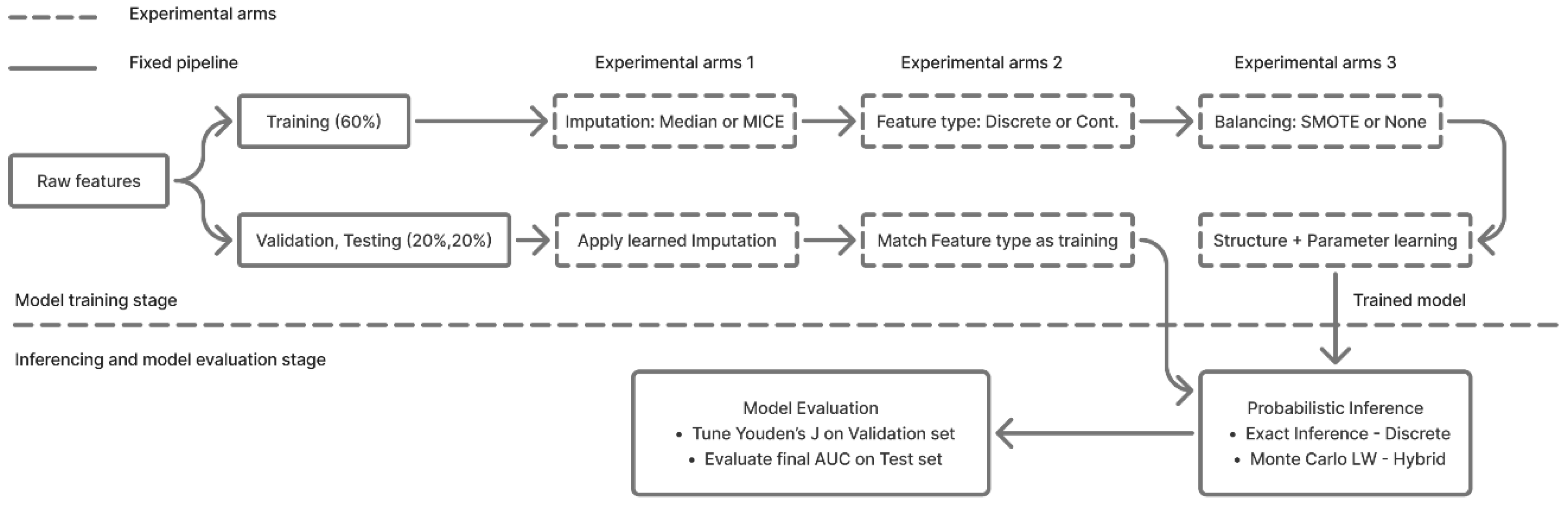
Figure 2.
Directed acyclic graph (DAG) of the optimal model (M6: MICE and continuous nodes).
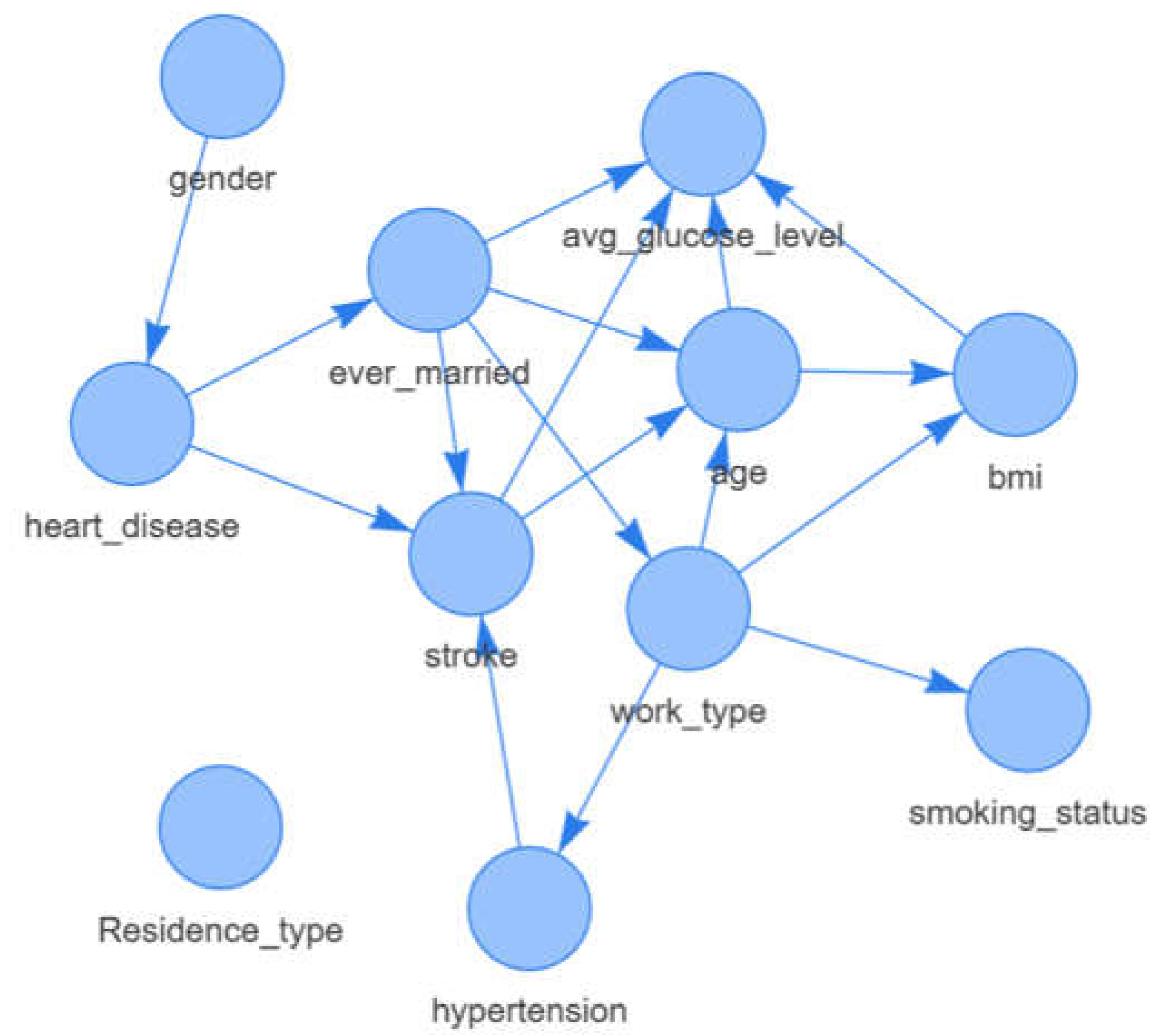
Figure 3.
ROC curve comparison of all experimental groups and the baseline data.
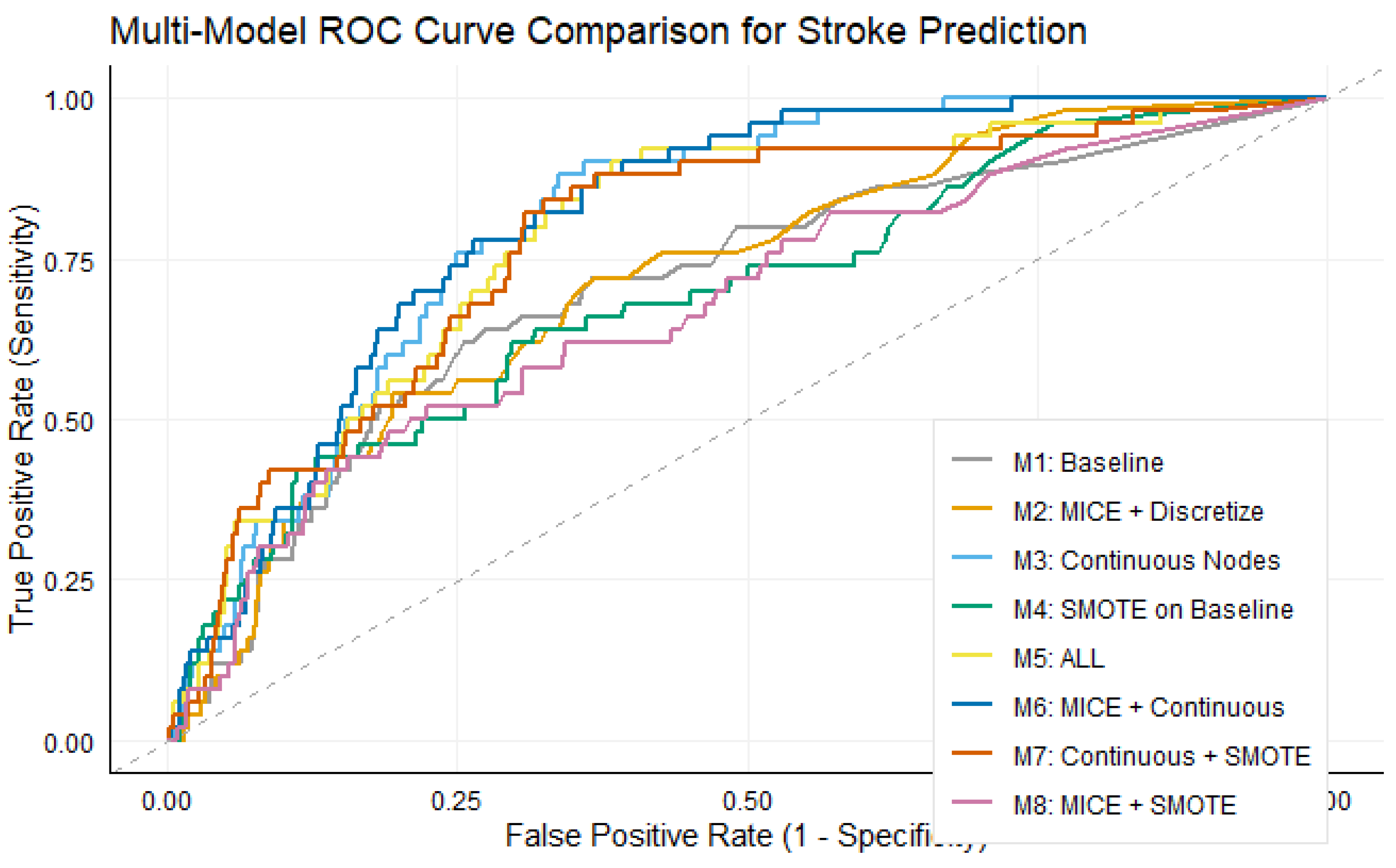
Figure 4.
Calibration (reliability) curves for four representative models. Observed stroke fraction versus mean predicted probability (deciles of predicted risk); the dashed diagonal denotes perfect calibration.
Figure 4.
Calibration (reliability) curves for four representative models. Observed stroke fraction versus mean predicted probability (deciles of predicted risk); the dashed diagonal denotes perfect calibration.
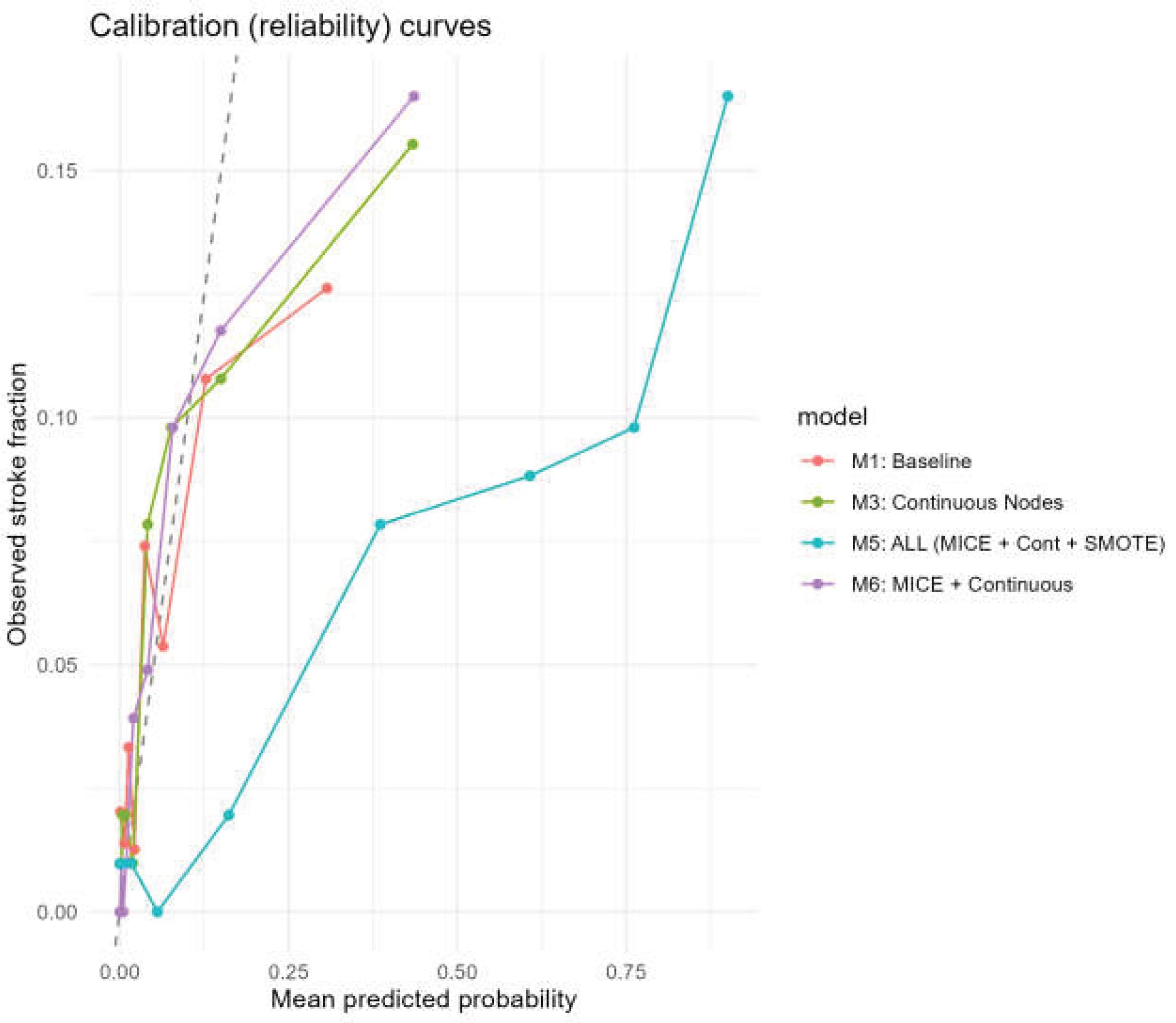

Table 1.
Study design arms 2x2x2 factors.
| Model | Arm 1: Imputation | Arm 2: Features | Arm 3: Balancing |
| M1 (Baseline) | Median | Discretized | None |
| M2 (MICE) | MICE | Discretized | None |
| M3 (Continuous) | Median | Continuous | None |
| M4 (SMOTE) | Median | Discretized | SMOTE |
| M5 (MICE + Cont. + SMOTE) | MICE | Continuous | SMOTE |
| M6 (MICE + Cont.) | MICE | Continuous | None |
| M7 (Cont. + SMOTE) | Median | Continuous | SMOTE |
| M8 (MICE + SMOTE) | MICE | Discretized | SMOTE |
Table 2.
Distribution of features in stroke and nonstroke patients with statistical significance.
| Feature | Stroke (n=249) | Non-Stroke (n=4861) | p value |
| Gender | Female: 141 (56.6%) | Female: 2853 (58.7%) | 0.5598 |
| Age | 67.73 ± 12.73 | 41.97 ± 22.29 | <0.001* |
| Hypertension | 0: 183 (73.5%) | 0: 4428 (91.1%) | <0.001* |
| Heart Disease | 0: 202 (81.1%) | 0: 4631 (95.3%) | <0.001* |
| Marital status | Yes: 220 (88.4%) | Yes: 3133 (64.5%) | <0.001* |
| Work Type | Private: 149 (59.8%) | Private: 2775 (57.1%) | <0.001* |
| Residence Type | Urban: 135 (54.2%) | Urban: 2461 (50.6%) | 0.2998 |
| Avg. Glucose Level | 132.54 ± 61.92 | 104.79 ± 43.85 | <0.001* |
| BMI | 30.47 ± 6.33 | 28.82 ± 7.91 | <0.001* |
| Smoking Status | never smoked: 90 (36.1%) | never smoked: 1802 (37.1%) | <0.001* |
Table 3.
Conditional probability table of the stroke with discrete variables.
| Heart Disease | Hypertension | Ever Married | Probability of Stroke |
| 0 | 0 | No | 1.19% |
| 0 | 0 | Yes | 5.14% |
| 0 | 1 | No | 13.33% |
| 0 | 1 | Yes | 10.88% |
| 1 | 0 | No | 15.38% |
| 1 | 0 | Yes | 12.96% |
| 1 | 1 | No | 75.00% |
| 1 | 1 | Yes | 13.33% |
Table 4.
Conditional probability table of stroke with continuous variables. (SD: Standard Deviation).
Table 4.
Conditional probability table of stroke with continuous variables. (SD: Standard Deviation).
| Stroke | Married | Intercept (β0) | Age Coefficient (β1) | BMI Coefficient (β2) | SD (σ) |
| 0 | No | 89.56 | 0.298 | 0.016 | 31.90 |
| 0 | Yes | 37.22 | 0.697 | 1.137 | 46.50 |
| 1 | No | 13.31 | 0.497 | 2.370 | 53.84 |
| 1 | Yes | -11.67 | 1.027 | 2.500 | 59.87 |
Table 5.
Performance metrics of all the models ranked by AUC (95% CI), then Youden’s J.
| Model | AUC (95% CI) | Youden's J | Sensitivity | Specificity |
| M6: MICE + Continuous | 0.812 (0.760-0.856) | 0.4672 | 0.78 | 0.6872 |
| M3: Continuous Nodes | 0.803 (0.755-0.848) | 0.4744 | 0.78 | 0.6944 |
| M5: ALL (MICE + Cont. + SMOTE) | 0.784 (0.719-0.838) | 0.4881 | 0.84 | 0.6481 |
| M7: Continuous + SMOTE | 0.781 (0.717-0.842) | 0.3326 | 0.56 | 0.7726 |
| M2: MICE + Discretize | 0.720 (0.652-0.784) | 0.3093 | 0.62 | 0.6893 |
| M1: Baseline | 0.718 (0.647-0.786) | 0.3038 | 0.56 | 0.7438 |
| M8: MICE + SMOTE | 0.692 (0.615-0.764) | 0.2782 | 0.52 | 0.7582 |
| M4: SMOTE on Baseline | 0.684 (0.603-0.758) | 0.2691 | 0.66 | 0.6091 |
Table 6.
Robustness of discrimination across 30 stratified resamples (mean ± SD test AUC).
| Arm | Mean AUC | SD |
| M1: Baseline | 0.770 | 0.039 |
| M2: MICE + Discretize | 0.769 | 0.040 |
| M3: Continuous Nodes | 0.821 | 0.028 |
| M6: MICE + Continuous | 0.820 | 0.028 |
Disclaimer/Publisher’s Note: The statements, opinions and data contained in all publications are solely those of the individual author(s) and contributor(s) and not of MDPI and/or the editor(s). MDPI and/or the editor(s) disclaim responsibility for any injury to people or property resulting from any ideas, methods, instructions or products referred to in the content. |
© 2026 by the authors. Licensee MDPI, Basel, Switzerland. This article is an open access article distributed under the terms and conditions of the Creative Commons Attribution (CC BY) license (http://creativecommons.org/licenses/by/4.0/).
Copyright: This open access article is published under a Creative Commons CC BY 4.0 license, which permit the free download, distribution, and reuse, provided that the author and preprint are cited in any reuse.


