

Submitted:
07 July 2026
Posted:
09 July 2026
You are already at the latest version
Abstract
This paper studies the optimal tax-and-transfer policy when automation raises productivity but displaces unskilled workers. Using a general equilibrium model calibrated to the U.S. economy, we compute the steady-state social welfare-maximizing rate of each of four tax instruments: capital income taxation, unskilled wage taxation, taxation on automation capital (i.e., a robot tax), and consumption taxation. Following an increase in the productivity of automation-related capital, the welfare-maximizing capital income tax rate is small, and the welfare-maximizing robot tax rate is zero at the baseline labor-automation elasticity because their long-run investment distortions largely offset their redistributive social benefits. In the baseline simulation, aggregate welfare is maximized by lowering the unskilled wage tax rate and/or raising the consumption and capital income tax rates, whilst the social welfare improvement is always the largest for optimal consumption taxation. When unskilled labor and automation-related capital are highly substitutable, the optimal consumption tax rate increases, and the additional government revenue is redistributed to displaced unskilled workers.
Keywords:
automation
; optimal taxation
; capital income tax
; labor income tax
; consumption tax
; robot tax
1. Introduction
Technological progress has long been a key driver of economic growth. Recent advances in automation and artificial intelligence (AI), however, have heightened concerns that productivity gains may come with greater inequality, especially when new technologies substitute for tasks performed by less-skilled workers (Lankisch et al., 2019; Jaimovich et al., 2021; Moll et al. 2022; Acemoglu, 2023; Tyers and Zhou, 2023; Brezis and Rubin, 2024). A central policy question is how the tax-and-transfer system should respond when automation shifts income toward capital owners and skilled workers while reducing the welfare of unskilled workers.
This paper answers this question in a general equilibrium model calibrated to the U.S. economy. The model features four fiscal instruments that are especially relevant in the automation era: (i) capital income taxation, (ii) labor income taxation of unskilled workers, (iii) taxation on automation-related capital (a “robot tax”), and (iv) consumption taxation. Following an increase in the productivity of automation-related capital, we compute the steady-state social welfare-maximizing rate for each tax instrument in turn, holding the remaining tax rates at their benchmark values. This exercise allows us to compare how each tax distorts capital accumulation and the adoption of automation and influences labor markets while redistributing resources across skilled workers, unskilled workers, and capitalists.
The analysis delivers three main results. First, capital income taxation and robot taxation are weak instruments for improving aggregate welfare in the new steady state. The welfare-maximizing capital income tax rate is small, and the associated welfare gain is quantitatively negligible, while the welfare-maximizing robot tax rate is zero. These taxes can redistribute some gains from automation to unskilled workers, but they also distort the accumulation of productivity-enhancing inputs. Second, in the baseline case, aggregate welfare is maximized by lowering the unskilled labor income tax rate, even though this reform is not Pareto-improving and can reduce the welfare of displaced unskilled workers. This stems from the unexpected mechanism by which welfare gains for skilled workers and owners of capital from automation-related technological progress more than offset the worsened welfare of unskilled workers when aggregated at the national level. Third, in this restricted one-instrument exercise, the consumption tax generates the largest aggregate welfare gain. This result is driven by the combination of a broad tax base and targeted transfers to unskilled workers under the maintained fiscal closure, rather than by a literal recommendation for a high statutory consumption tax rate. When unskilled labor and automation-related capital are more highly substitutable, the optimal consumption tax rate rises further to strengthen the redistribution mechanism under massive displaced unskilled workers.
The key mechanism is that automation-related capital substitutes for unskilled labor in production. As productivity rises, firms adopt more automation capital, reducing the demand for unskilled labor and shifting income toward skilled workers and capital owners. Fiscal instruments, therefore, affect welfare not only through redistribution but also through capital accumulation, factor prices, and the extent of technological displacement. Without automation, the model would miss the main channel through which recent technological progress alters inequality. A standard model with only conventional capital cannot capture the substitution of machines for unskilled labor, the associated decline in unskilled wages, or the role of a tax on automation capital. Moreover, policies targeting capital or labor income taxes and consumption taxes would be evaluated without accounting for how automation reshapes factor substitutability. As a result, it would provide an incomplete basis for evaluating optimal tax policy in the era of automation.
In our model, the trade-off between production efficiency and equity among different types of agents makes optimal taxation policy different from the economy without automation, which introduces a new input that can substitute for unskilled labor. A tax on capital income or on automation capital does more than redistribute income from capital owners; it also shifts the margin at which firms replace unskilled workers with machines. This creates a new trade-off relative to standard optimal tax problems. Higher taxes on capital or robots may protect workers through redistribution, but they also discourage the accumulation of these inputs that raise productivity. In contrast, a uniform consumption tax does not directly alter the factor mix, so it can redistribute wealth with smaller effects on automation adoption. Without automation, the model would collapse to a more conventional capital-labor environment in which there is no separate technology margin between unskilled labor and machines. One could still study the standard efficiency cost of capital taxation but not the distinct question of whether the input that displaces workers should be taxed differently from other capital or how the answer depends on labor-automation substitutability and the speed of automation-augmented technological progress. Automation is therefore not an ornamental extension: it is the feature that makes the ranking of capital, robot, labor-income, and consumption taxes quantitatively interesting.
This paper contributes to four related literatures. First, it adds to the growing body of work on robot (and AI) taxation and automation policy, which analyzes whether and when automation capital should be taxed and how such policies interact with income taxation (e.g., Stiglitz, 2018; Zhang, 2019; Guerreiro et al., 2022; Thuemmel, 2023; Costinot and Werning, 2023; Growiec et al., 2026; Korinek and Stiglitz, 2026). We find that the optimal robot tax rate is (around) zero unless robots and AI become more highly substitutable with workers than the current situation. Relative to this work, we expand the policy menu to include capital and labor income and consumption taxation and provide a quantitative comparison of these instruments within a unified general equilibrium framework.
Second, our results speak to the long-run capital income taxation debate (Judd, 1985; Chamley, 1986; Judd, 2002; Domeij 2005; Abel, 2007; Straub and Werning, 2020) by showing that, in an economy where automation raises the return to capital, the welfare-maximizing long-run tax rate on capital remains quantitatively low, reflecting investment distortions taken into account, unless the elasticity of substitution between automation and labor becomes higher from the status-quo level (or the speed of autonomous technological progress becomes faster).
Third, our analysis relates to the literature on optimal commodity taxation (Atkinson and Stiglitz, 1976; Naito, 1999) by highlighting that the welfare role of a uniform consumption tax can be sensitive to technology–labor substitutability in an automated economy. Additionally, our research demonstrates that consumption taxation is the most useful tax policy instrument to redistribute gains from automation due to its least distortive features on technological progress.
Fourth, we build on the quantitative automation framework of Berg et al. (2018) and Berg et al. (2021), focusing on steady-state optimality and comparing alternative tax instruments under a balanced-budget requirement with targeted transfers.
2. The Model
The economy consists of firms, skilled and unskilled workers, owners of capital (or capitalists), and the government. The numbers of skilled workers, unskilled workers, and capitalists are denoted by , , and , respectively. Without a loss of generality, we normalize the total population to one. Thus, The population shares are constant over time. Time is discrete and indexed by = 0, 1, 2, ….
There are three types of firms: intermediate goods firms, final goods firms, and wholesalers. The production of intermediate goods requires the combination of traditional capital , automation-related capital (which comprises robots and intangible capital related to AI. Intangible capital includes AI and its associated production components such as software, licenses, patents, copyrights, and big data (Nakatani, 2024). Such a way to include both robots (autonomous capital) and AI (intelligent capital) as a combined automation-related capital is becoming a popular approach in modeling (Casas and Torres, 2023).) , skilled labor , and unskilled labor .
Final goods. The final goods are produced by combining a continuum of differentiated goods indexed by , according to the Dixit and Stiglitz (1977) aggregator:
where is the quantity of output sold by wholesale firm and where is the elasticity of substitution across the differentiated goods, satisfying . The final goods producer maximizes profits as subject to the above production technology, taking the input price and the final goods price as given. The profit maximization problem yields the following demand function:
and the aggregate price index . Without a loss of generality, we normalize the output price to one, i.e., .
𝑦𝑗,𝑡=p𝑗,𝑡/𝑃𝑡−𝜖𝑌𝑡,
Wholesalers and markups. There is a unit measure for wholesalers. They purchase homogeneous intermediate goods from intermediate-goods firms and transform them into heterogeneous final goods, which are then sold to final-goods firms. Their production technology is linear: . We assume that wholesalers are owned by capitalists and have monopolistic power to set the price of the goods they sell. This assumption reflects the fact that large tech companies enjoy monopolistic rent in the age of automation/AI/big data. Recent work suggests that automation and digital technologies can reinforce economies of scale and contribute to the rise of superstar firms (Firooz et al., 2025), while market share concentration and resulting markups have also increased in wholesale-related activities (Hsieh and Rossi-Hansberg, 2023; Ganapati, 2025). Thus, automation should be modeled with markups (Auray and Eyquem, 2025).
Given this, the representative wholesaler chooses and to solve the following problem:
which is subject to the demand function (2). is the price of intermediate goods. Then, we have
and by normalizing the price of final goods to unity and assuming a symmetric equilibrium, equation (4) yields
Note that the markup can be expressed asWe assume that the markup is constant. We introduce markup because large firms (e.g., big tech companies) can take advantage of owning the platform and other digitalization-related networks, which makes their marginal costs lower than the average costs (Nakatani, 2023). This is because the costs of constructing such a network can be an entry barrier for other companies, which leads to both large market shares and markups.
Intermediate production. The intermediate goods firm produces output by using traditional capital , automation capital (e.g., robots) , Investments in AI and robotics, both part of automation capital, have different spillover effects. Robotics involves physical hardware and strict safety regulations, mainly used in manufacturing, logistics, and surgery. AI, with fewer physical constraints, develops faster and offers intelligence across diverse digital and service sectors like finance and autonomous driving. skilled labor , and unskilled labor , according to the following triple-nested constant elasticity of substitution (CES) production function:
where is the aggregate productivity and
where is the elasticity of substitution between composite inputs and , is the elasticity of substitution between automation capital and unskilled workers, and is the elasticity of substitution between traditional capital and skilled labor. Depending on the values of these elasticities, this production technology allows for high substitution between unskilled labor and robots and complementarity between (un)skilled labor and traditional capital (Krusell et al., 2000) as well as between skilled labor and robots. Automation technologies displace certain worker groups from jobs for which they have a comparative advantage (Acemoglu and Restrepo, 2022). In our model, this displacement falls on unskilled workers. In practice, automation capital may be interpreted as industrial robots or related automation technologies.
The intermediate goods firm maximizes its profit by choosing capital, robots, and two types of labor, subject to equations (6)-(8) according to
where and are the rental rates of capital and robots, respectively, and where and are the wage rates for skilled and unskilled workers, respectively. The first-order conditions of this problem are as follows:
Households. Workers consume all of their income. The representative skilled worker’s utility function is calculated by preferences as proposed by Greenwood et al. (1988) to abstract from income effects. If we introduce the income effects, the main resulting change would be that skilled labor decreases in response to technological progress (i.e., an increase in the productivity of automation technology). Such a difference occurs because under the separable utility function, the labor supply will depend not only on real wages but also consumption.:
where is the consumption of skilled workers and is their labor supply. We do not study the friction in the labor matching market. See Guimarães and Gil (2022), Charalampidis and Guillochon (2025), Kudoh and Miyamoto (2025), and Charalampidis and Razafitsiory (2025), for such topic in the context of automation. is a measure of the disutility parameter of working, and is the inverse of the Frisch elasticity. Since we know from Diamond (1998) that the optimal marginal tax rate at the bottom of the skill distribution becomes higher when there are no income effects on the utility function, we prefer this specification of the utility function to examine whether the progressive labor income tax rate is still optimal in this robust setting. The budget constraint of the skilled worker is
where is the consumption tax rate, is the tax rate on skilled workers’ income, and is the universal lump-sum transfer. The skilled worker chooses and to maximize the utility function in (12) subject to the budget constraint in (13). The hand-to-mouth assumption for skilled workers mirrors the U.S. economy, where many households, even high-income workers, lack sufficient savings for emergencies (American Bankruptcy Institute, 2016) due to spending all income and limited financial capability (Despard et al., 2020). The first-order conditions correspond to equation (13), and
Similarly, the unskilled worker’s problem can be written as
which is subject to
where is the tax rate on unskilled workers’ income and is the targeted transfer to unskilled workers. The first-order conditions are modeled by equation (16) and
Capitalists own firms, do not work, and save money to smooth consumption over time. These savings are invested in automation and traditional capital. This setup helps characterize the “winner-take-all” aspect of automation as well as the fact that “the rise of the top one percent is likely very tied up with technology.” In other words, the benefits of new automation technologies accrue to owners of capital in the form of higher capital incomes (Moll et al., 2022). The representative capitalist chooses consumption , investment in traditional capital , and investment in automation to maximize
subject to the following budget constraint and the capital and robot accumulation equations:
And
where is the discount factor, is the depreciation rate of capital, is the depreciation rate of the robots, is the capital income tax rate, is the tax rate on markup, and is the robot tax rate.
The first-order conditions of the capitalists’ maximization problem include the following Euler equations:
and
which at the initial steady state correspond to
and
Government. The government has multiple instruments (taxes and expenditures) with which to implement fiscal policy, subject to a balanced budget in each period. If the government borrows to fund transfers to unskilled workers, it makes sense to borrow initially and repay after automation-driven growth expands the economy and tax revenues. However, larger debt raises interest rates, boosting returns on traditional and automation capital but slowing technological progress due to higher borrowing costs. Government borrowing may also crowd out private investment in traditional and automation-related capital. Although capitalists could enjoy higher returns from such investments, expectations of future tax hikes to repay debt could trigger Ricardian effects, as government debt must eventually be repaid through higher tax revenues. The government budget constraint is given by
In the initial equilibrium, collected total tax revenues are redistributed to three agents (unskilled workers, skilled workers, and capitalists) equally as a universal lump-sum transfer . In the initial steady state, we set sL=0. Given the calibrated tax rates, the universal lump-sum transfer κ is then determined residually from the government budget constraint. In the post-automation benchmark and in all counterfactual tax experiments, we keep κ fixed at its initial steady-state value and let the targeted transfers to unskilled workers adjust residually. This can be interpreted as a situation where the government provides universal lump-sum transfers equally to all citizens without any particular redistribution purpose in the initial steady state. Then, after a realization of shock to automation technology, the government redistributes additional tax revenues as targeted transfers to unskilled workers, who suffer from automation-related technological advancement. We impose a nonnegative constraint for targeted transfers to unskilled workers:
Equilibrium. The goods market is in equilibrium when the supply of firms equals the demand of capitalists, workers, and the government:
The labor markets are in equilibrium when the labor demand is equal to the labor services supplied by workers:
and
Similarly, the capital and robot markets are in equilibrium when the demands equal the supplies:
and
Welfare. The welfare gain for skilled workers , as defined by Domeij and Heathcote (2004), satisfies the following equation:
where equilibrium consumption is represented by in the case of tax reform and in the case of no tax reform. The same applies to superscripts of labor supply. The above equation can be rewritten as follows:
The same calculation yields a welfare gain for unskilled workers :
The welfare gain for capitalists satisfies the following equation:
Social welfare based on population shares, as introduced by Acemoglu and Autor (2011), is defined as follows:
3. Calibration
The model is calibrated to match the U.S. economy. Table 1 summarizes the parameter values for the initial steady state. Following Berg et al. (2018), we set the annual discount rate to 6 percent, implying the discount factor . The depreciation rate is higher for robots than for traditional capital, with and .
The shares in production of the composite input , unskilled labor , and skilled labor are calibrated to match a capital income share of 0.35, an unskilled labor income share of 0.31, a skilled labor income share of 0.30, and a robot income share of 0.04. This yields = 0.772, = 0.964, and = 0.092. Following Berg et al. (2018), we set the elasticity of substitution between and to 0.67 and the elasticity of substitution between skilled labor and capital to 0.335. We set the elasticity of substitution between unskilled labor and robots to 1.9, as estimated by DeCanio (2016). This is a reasonable value for our baseline simulation because Adachi (2025) found that the elasticity of substitution between robots and labor is heterogeneous across occupations, with the mean value of 2.05, reaching up to 3 in production and material moving occupations in Japan, where the robot adoption rate is higher than the U.S. When the elasticity of substitution is less (greater) than one, two inputs are gross complements (substitutes). means that skilled labor and robots are gross complements and that unskilled labor and traditional capital are also gross complements. In contrast, indicates that robots and unskilled labor are gross substitutes. The markup is set to 1.21, based on Barkai (2020), for 2014.
For the inverse of the Frisch elasticity, we set and , which are taken from the intensive margin as per Chetty et al. (2011). This means that the Frisch elasticity of both unskilled and skilled labor is 0.5, which is the median value suggested in the literature. Following Berg et al. (2018), we set the intertemporal elasticity of substitution to 0.5 (i.e., ), which is the same as the mean estimated by Havranek et al. (2015). The disutility parameter of working for unskilled workers is set by targeting the steady-state working hours to be one-third (i.e., eight hours per day). The steady-state wage premium for the U.S. economy—i.e., —is used to specify that the parameter of skilled workers’ disutility from working because a steady-state skill premium depends on the difference in the advantage of skilled workers over unskilled workers (Afonso et al., 2023).
The population is normalized to 1, and the share of capitalists is one percent. When studying wealth and income distribution, focusing on the top one percent of income earners is a common approach (Alvaredo et al., 2013; Saez and Zucman, 2020). We use this group to represent capitalists, justified by Saez’s (2017) finding that they notably adjust reported income based on the net-of-tax rate, mainly through capital gains and dividends, which our model proxies as capital income. The share of skilled workers to total workers is 45 percent, as reported by Acemoglu and Autor (2011).
We calibrate the tax rates using the latest 2014 U.S. national accounts data. The labor income tax rate is set so that individual income tax revenue equals 9.3 percent of GDP, which is the actual ratio of personal income tax revenue to GDP. The capital income tax rate is set so that capital gains tax revenue equals 0.7 percent of GDP, which is the actual ratio of capital gains tax revenue to GDP. The markup tax rate is set so that corporate income tax revenue equals 1.8 percent of GDP, which is the actual corporate income tax revenue as a percentage of GDP. The consumption tax rate is calibrated to match the actual ratio of 4.5 percent, representing indirect tax revenue (taxes on goods and services and on international trade) as a share of GDP. This procedure implies for labor income taxation, for capital income taxation, for taxation on markup, and for consumption taxation. Note that all collected tax revenues are used for universal lump-sum transfers in the initial steady state. This fiscal closure yields = 0.163 in the initial steady state. Under benchmark tax rates after the 50 percent automation-productivity increase, the residual targeted transfer is = 0.0162 per unskilled worker.
4. Results
As a benchmark, we first examine how social welfare and key macroeconomic variables respond to changes in tax rates in the absence of technological progress in automation. The results are reported in the Appendix. The consumption tax is the most powerful tax policy tool for influencing social welfare, without affecting the wage premium. In contrast, capital income and unskilled wage taxes affect redistribution by changing the wage premium.
In the baseline automation experiment, we focus on steady states and consider a 50 percent increase in the productivity of automation-related capital. For each instrument, we vary one tax rate while holding the remaining tax rates at their status-quo levels and adjust targeted transfers to unskilled workers in order to satisfy the balanced budget constraint, subject to a nonnegativity constraint on the transfers. We refer to the resulting reform as “optimal” for that instrument if it maximizes social welfare. The results are shown in Figure 1, Figure 2, Figure 3 and Figure 4, in which the horizontal axis shows the level of the tax rate and the vertical axis shows the welfare change from tax reform relative to the situation without tax reform, as discussed below.
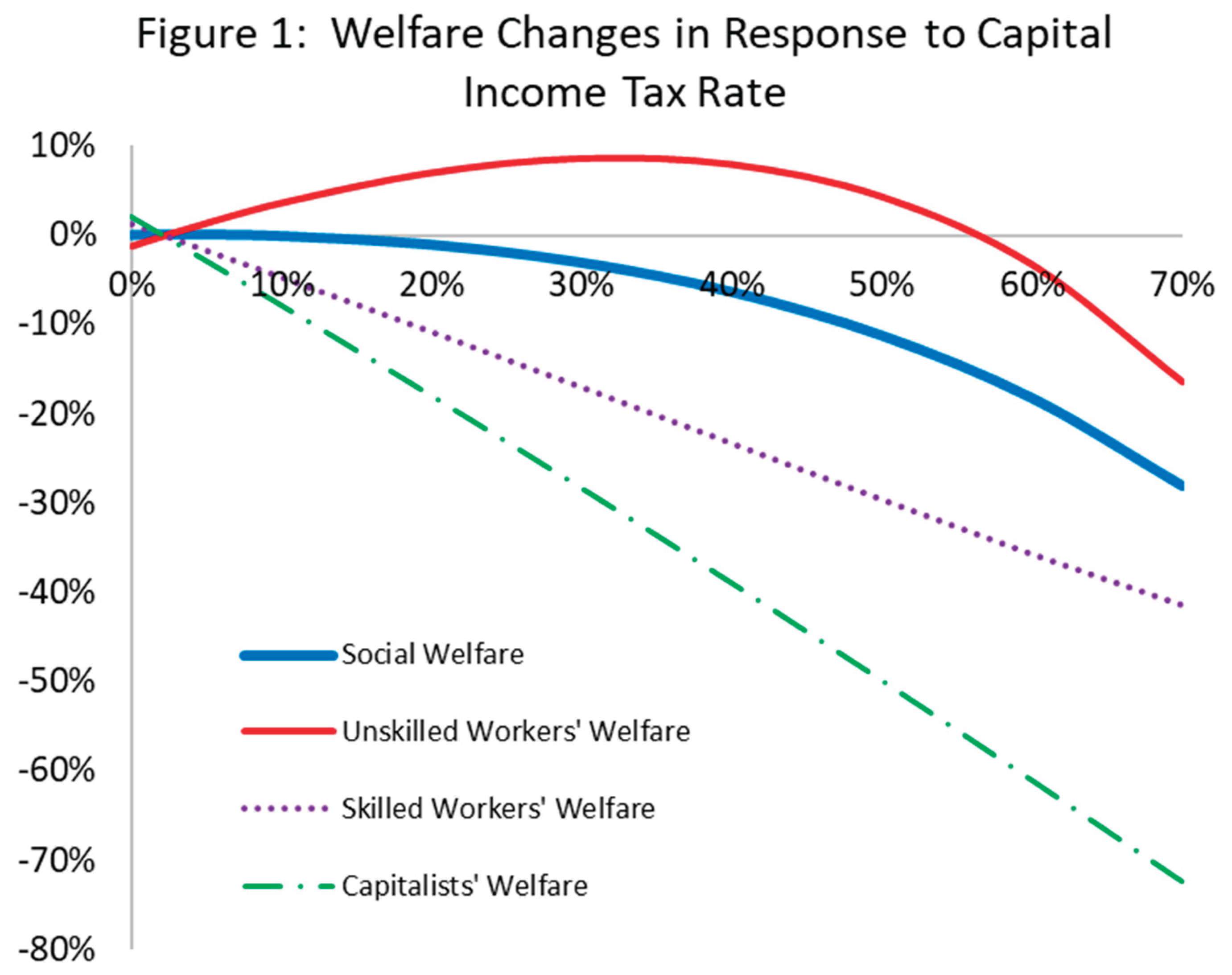
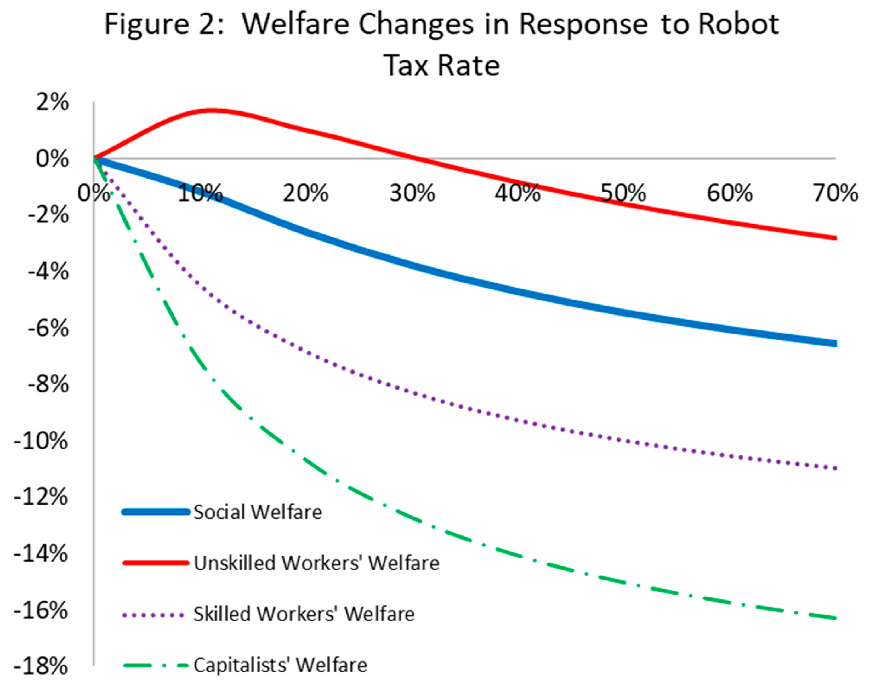
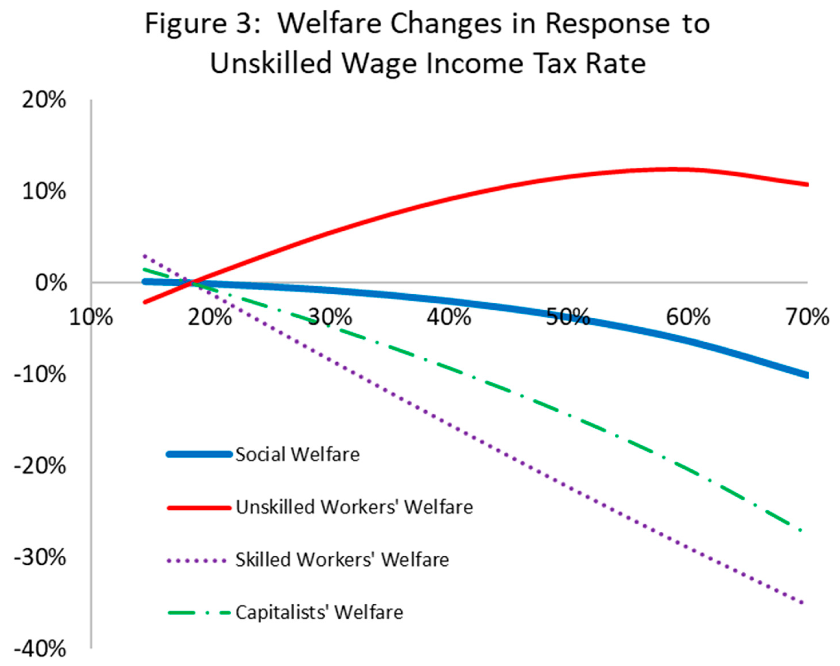
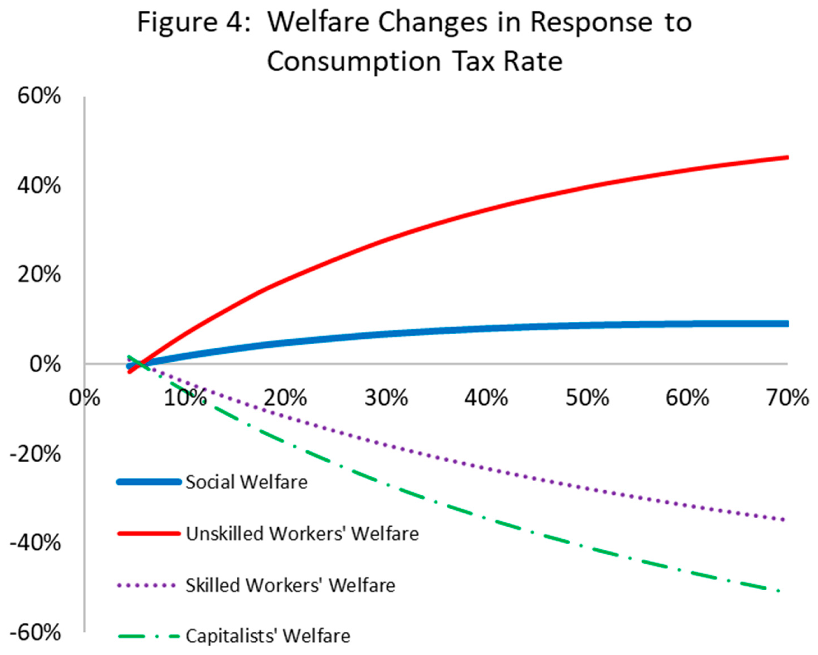
Figure 1 shows that capital income taxation affects unskilled workers’ welfare through three channels. First, a higher capital income tax raises revenue for targeted transfers and shifts part of capitalists’ gains from automation to unskilled workers. This transfer channel raises unskilled workers’ consumption and welfare. Second, a capital income tax rate hike discourages the accumulation of automation-related capital. This reduces substitution away from unskilled labor, but it may also induce unskilled workers to supply more labor, increasing work disutility. Third, the tax reduces traditional capital accumulation. This matters because traditional capital and unskilled labor are gross complements through the outer nest of the CES production function. Hence, a decline in traditional capital reduces the marginal product of unskilled labor and partly offsets the transfer gain. Overall, the transfer channel dominates locally, but the capital-accumulation and complementarity channels keep the aggregate welfare gain very small.
In the aggregate, social welfare is maximized at a 3.6 percent capital income tax rate in the new steady state, which yields a negligible 0.01 percent consumption-equivalent gain relative to the status quo. This rate is 1.5 percentage points above the initial-steady-state optimum. Moving from the benchmark tax rate to this optimum lowers the welfare of capitalists and skilled workers because it slows down the pace of capital accumulation, but the resulting gains to unskilled workers more than offset that loss.
The robot tax discourages the accumulation of automation-related capital, thereby limiting gains from automation-augmented technological progress. This lowers capitalists’ welfare while redistributing benefits from automation to unskilled workers through transfers (Figure 2). We find that the welfare gain is positive for unskilled workers at low robot tax rates. Since the tax on automation-related capital is very costly in the steady state, it is optimal not to impose such a tax, as shown in Figure 2. As shown in the figure, the individual welfare of unskilled workers is concave and even declines when the robot tax rate is very high. Our finding is consistent with Gasteiger and Prettner (2022), who reported that the robot tax cannot induce a takeoff toward positive long-run growth. Prettner and Strulik (2020) also reported that even the net income of high-skilled workers declines with the robot tax because the wage-depressing impact of reduced demand for machines and the complementary role of skilled workers apparently overcompensates for the gains from redistribution.
A reduction in the tax rate on unskilled workers’ wage income improves social welfare through the intra-temporal labor-supply margin (Figure 3). A lower unskilled wage tax raises the net-of-tax return to unskilled work. Under the Greenwood-Hercowitz-Huffman (1988) preferences used in the model, unskilled workers respond by voluntarily supplying more labor. This creates two opposing effects for them: after-tax labor income and consumption tend to rise, but the disutility from additional work also rises. In the baseline calibration, the work-disutility effect dominates, so unskilled workers’ consumption-equivalent welfare falls. Contrastingly, skilled workers and capitalists benefit from the expansion of production associated with greater unskilled labor input. As a result, the optimal tax rate is 14.3 percent. The social welfare gain from the optimal unskilled wage income tax is a 0.27 percent increase in the consumption equivalent, which is greater than the gain from optimal capital income taxation.
The model-implied optimal consumption tax rate is relatively high at 66.8 percent on a tax-exclusive basis (Figure 4), which is 3.8 percentage points higher than the optimal rate in the initial steady state. Expressed as a tax-inclusive rate, this corresponds to approximately 40 percent. A recent study by Casas and Torres (2024) found that the consumption tax rate should be 37.6 percent when the adoption rate of automation technology reaches 38 percent in the economy. Under the maintained fiscal closure, the universal transfer is fixed at its initial steady-state value, and residual revenues are redistributed to unskilled workers through the targeted transfer . The resulting increase in targeted transfers raises unskilled workers’ consumption-equivalent welfare sufficiently to outweigh the population-weighted welfare losses of skilled workers and capitalists. The social welfare gain from this optimal consumption tax reform, a 9.19 percent increase in consumption-equivalent terms, is the largest among the one-instrument tax reforms compared in Figure 1, Figure 2, Figure 3 and Figure 4. For tax rates above the optimum, the additional welfare losses of skilled workers and capitalists exceed the incremental welfare gains of unskilled workers. Therefore, the high model-implied rate should not be interpreted as a literal policy prescription. Rather, it is the outcome of a restricted one-instrument steady-state exercise: with fixed and adjusting residually, a higher consumption tax provides a broad tax base for financing targeted transfers to the group most adversely affected by automation, while avoiding the direct factor-income and investment wedges created by capital income and robot taxes.
To further understand the mechanisms and economic impacts, we compare the impacts on key economic variables. We specifically discuss the effects on output, the wage premium, and targeted transfers to unskilled workers under various optimal tax rates. We do not discuss the case of an optimal zero robot tax rate here because it corresponds to the status quo economy given that there is no robot tax in the initial steady state.
Regarding the impact on output, the optimal unskilled wage income tax shows the largest increase (1.4 percent relative to the new steady state without tax reform) because lower taxation of unskilled labor induces additional labor supply, raises firms’ demand for unskilled labor, and thereby expands production. The optimal capital income tax lowers output by 0.9 percent because it reduces the accumulation of both traditional and automation-related capital. Compared with this case of optimal capital income taxation, the output decrease under optimal consumption taxation is greater (-20.5 percent) due to the larger tax rate increase.
With respect to the distributional impacts, all three types of optimal taxation increase the wage premium in the new steady state from its initial value of 1.65. This is because improvements in automation productivity increase the demand for skilled labor more than for unskilled labor, thereby raising the skilled wage relative to the unskilled wage. Among the three optimal taxes considered, the optimal consumption tax notably demonstrates the highest wage premium of 1.76 compared with the other two cases of optimal taxation (1.75 for optimal capital income taxation and 1.73 for optimal unskilled wage income taxation).
Targeted transfers to unskilled workers are modest under optimal capital income taxation. For example, targeted transfers to unskilled workers under optimal capital income taxation constitute 6.9 percent of government revenue and 3.4 percent of unskilled workers’ income. Yet these targeted transfers are close to zero under optimal unskilled wage income taxation, as they face the nonnegativity constraint on transfers. In contrast, targeted transfers to unskilled workers account for 57.5 percent of their income under the optimal consumption tax due to its relatively high tax rate.
5. Sensitivity Analysis
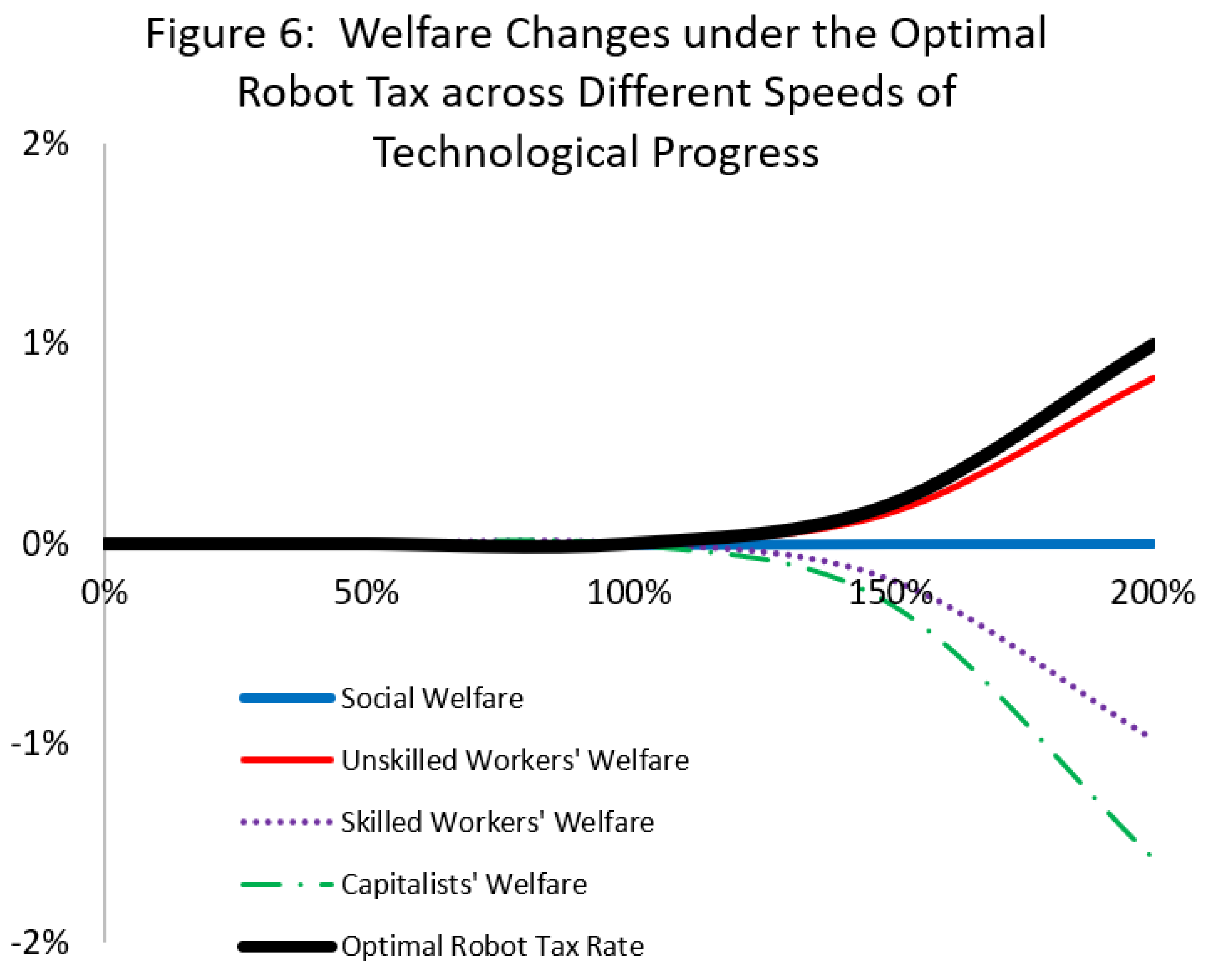
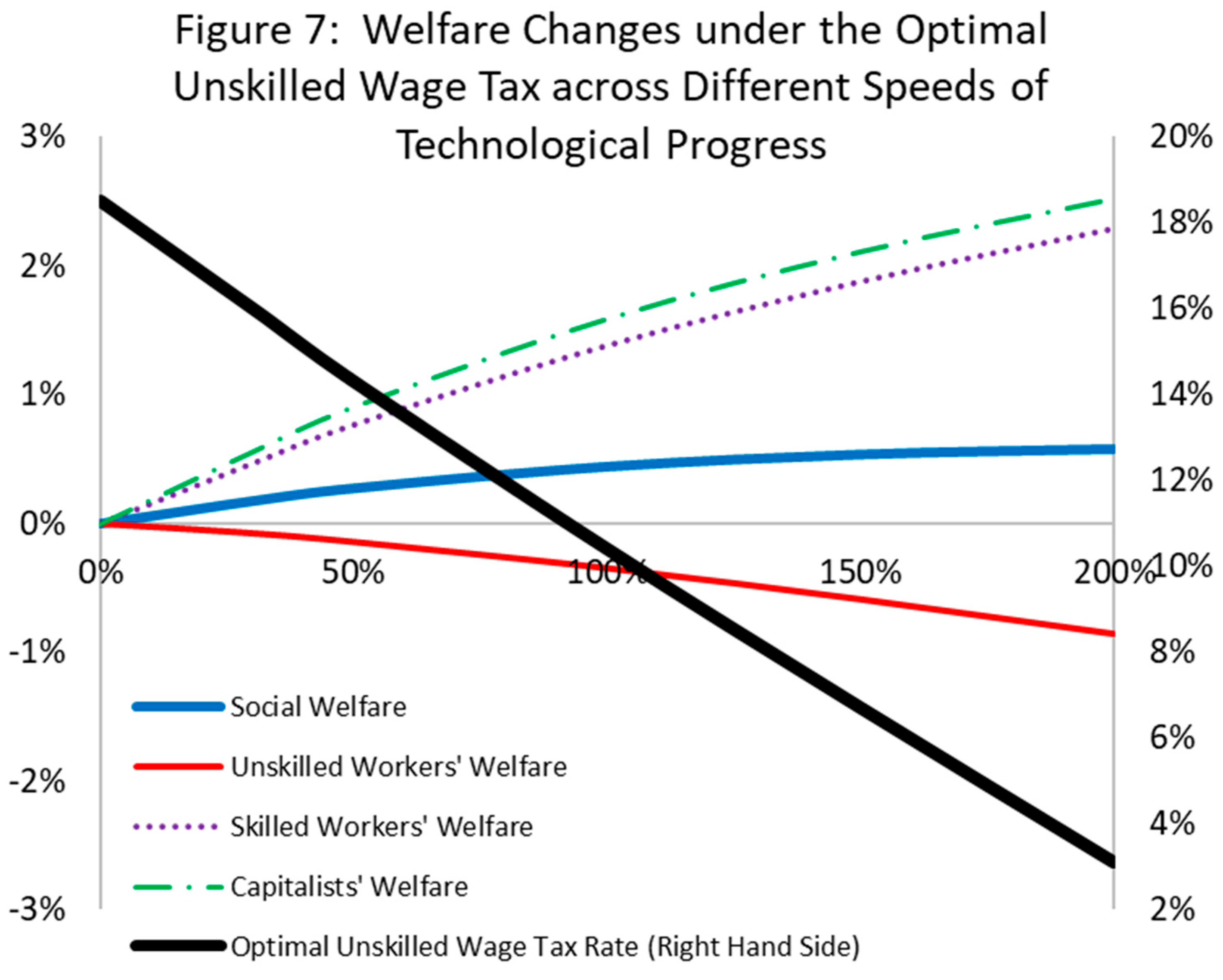
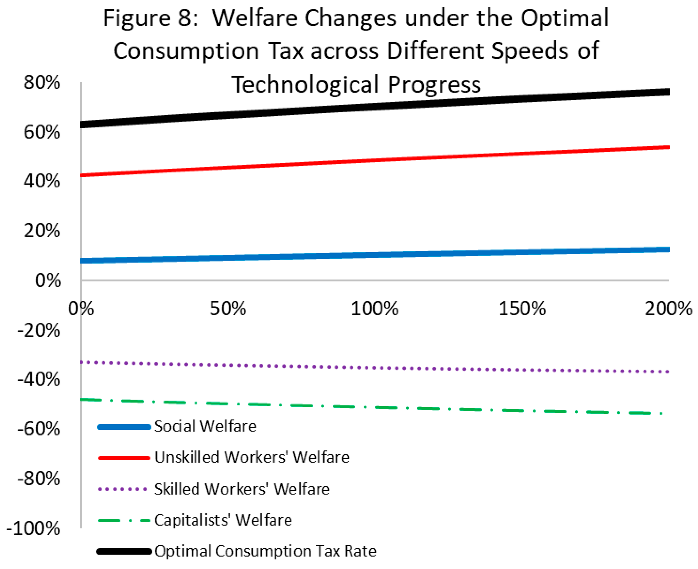
This section examines sensitivity to two particularly uncertain parameters: the size of automation-related technological progress and the elasticity of substitution between automation-related capital and unskilled labor. Figure 5, Figure 6, Figure 7 and Figure 8 report the results for alternative sizes of automation productivity improvement.
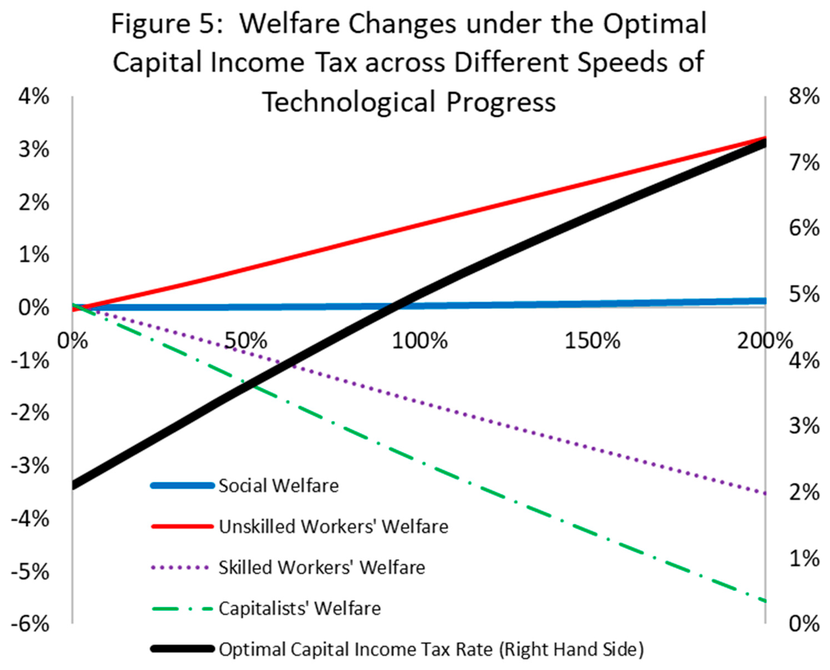
As the speed of automation-augmented technological progress becomes faster, the optimal capital income tax rate increases (Figure 5). This is to balance the trade-offs between redistributing more gains from automation toward suffering unskilled workers through targeted transfers and avoiding excessive detrimental effects on capital accumulation. Nevertheless, the aggregated social welfare change is negligible because the welfare gains for unskilled workers are offset by the welfare losses for capitalists and skilled workers (Figure 5).
An optimal robot tax rate becomes positive when the speed of automation becomes very fast (Figure 6). However, the optimal robot tax rate remains very low—such as 0.2 percent for a 150 percentage increase in automation productivity. Even in the case of a 200 percentage increase in automation productivity, the optimal robot tax rate is relatively low at 1.0 percent. The magnitude of optimal robot tax rate found in this exercise is very similar to the findings in the literature on optimal robot taxation. For instance, Thuemmel (2023) also found that the optimal robot tax rate is 1 percent at a maximum. This is due to the detrimental costly effects of robot tax on automation investment, which prevents society from reaping the benefits from automation. Similar to optimal capital income taxation, social welfare remains very close to zero, as unskilled workers’ welfare gain is offset by the other two agents.
Across different speeds of automation-related technological progress, changing the unskilled wage income tax rate delivers relatively modest aggregate welfare gains. This result can be attributed to the fact that monopolistic power increases the tax incidence borne by firms under automation, thereby making labor income taxes less effective at redistributing income than at redistributing profits. As the size of the technological shock increases, the government has more room to cut the unskilled wage income tax, satisfying the nonnegativity constraint of the targeted transfers (Figure 7).
Furthermore, it is optimal to increase the consumption tax rate in the automated economy because the welfare gain for unskilled workers exceeds the welfare losses for skilled workers and capitalists. By using additional consumption tax revenues, unskilled workers receive higher amounts of their targeted transfers, which improves their lives (Figure 8). The optimal consumption tax rate is set at the point where the welfare losses of capitalists and skilled workers do not offset the welfare gains for unskilled workers.
Next, we conduct sensitivity analysis regarding the elasticity of substitution between unskilled labor and automation-related capital (). We also examined the other values of the elasticity of substitution ( and ) in the production function, but the results did not change significantly. Following Berg et al. (2018), we consider values up to . Holding all other parameters fixed at their baseline values (Table 1), we change only the value of in the new steady state. The simulation results are shown in Table 2.
The optimal capital income tax rate becomes higher when the elasticity of substitution between unskilled labor and automation-related capital becomes higher. An economic intuition is that when unskilled workers are more displaced by automation-related capital, the government should tax more on capital and transfer those revenues toward displaced unskilled workers. Although the optimal capital income tax rate is always higher than the optimal robot tax rate irrespective of the elasticity of substitution, both tax rates increase nonlinearly in a concave way under extremely high elasticity of substitution due to their distortion of capital accumulation. We found that optimal capital income taxation shows the second largest social welfare gain next to the optimal consumption taxation in this exercise of different values of elasticity of substitution.
Optimal robot taxation depends on the elasticity of substitution between automation capital and unskilled labor. When the elasticity becomes higher, the optimal robot tax rate nonlinearly increases toward 10 percent in the case of the highest value of elasticity . This is because such elasticity is critical for determining the displacement effects of automation on unskilled workers, so social welfare becomes highly sensitive to the welfare improvement of unskilled workers. However, owing to the distortionary nature of the robot tax, the optimal tax rate remains relatively low, below 10 percent, compared to other types of taxes, such as the optimal consumption tax rate discussed below.
Regarding optimal labor income taxation, as the elasticity of substitution between automation-related capital and unskilled labor increases, the government should lower the tax rate on unskilled wage income more. Specifically, by cutting the labor income tax rate for unskilled workers, the tax burden for unskilled workers decreases, and the targeted transfers can be financed more by other tax instruments, such as capital income tax revenues. The additional tax revenues can be redistributed to unskilled workers, thereby increasing their consumption and raising their welfare. However, the welfare gain from changing taxes on unskilled workers’ income remains negligible, especially when the elasticity of substitution between automation-related capital and unskilled labor becomes higher.
Finally, the optimal consumption tax response is highly sensitive to the elasticity of substitution between unskilled labor and automation-related capital. A higher consumption tax raises revenue from a broad tax base that includes all consumers. Under the maintained fiscal closure, the additional revenue is redistributed to unskilled workers through the targeted transfer. When the labor-automation elasticity is high, the redistributive gains for unskilled workers become large enough to dominate the welfare losses of skilled workers and capitalists.
6. Conclusions
This study evaluates how standard tax instruments perform as tools for redistribution and welfare maximization when automation-related productivity rises. Focusing on steady-state outcomes and imposing a balanced-budget requirement, the government adjusts transfers—targeted to unskilled workers and subject to a nonnegativity constraint—to finance each tax reform. This environment clarifies how different taxes trade off redistribution against long-run efficiency, as automation increases inequality.
Our main results show that under the maintained one-instrument fiscal experiments, consumption taxation generates the largest consumption-equivalent welfare gain among all tax reforms considered, driven by sizable improvements in the consumption of unskilled workers. This result should not be read as a literal recommendation for a very high statutory consumption tax rate. Rather, it highlights that when targeted transfers to displaced workers are available, a broad consumption-tax base can finance redistribution with smaller direct distortions to automation and capital accumulation than capital income or robot taxation.
In contrast, the role of robot taxation is limited in an automated economy because the efficiency losses from the tax outweigh their redistributive benefits in most scenarios. Robot taxation becomes a useful tool only when the elasticity of substitution between robots and unskilled labor becomes much higher than the status quo in the future.
Although a higher capital income tax transfers some automation gains from capitalists (and skilled workers) to unskilled workers, the overall social welfare improvement is negligible. However, similar to optimal robot taxation, optimal capital income taxation can be an effective tool when the elasticity of substitution between unskilled labor and automation capital increases from the status-quo level in the future. In such a case, optimal capital income taxation brings larger social welfare benefits than optimal robot taxation due to its broader tax base.
The unskilled wage income tax plays a more nuanced role. Reducing this tax rate raises the net-of-tax return to unskilled labor and induces unskilled workers to supply more labor. In the baseline calibration, their consumption gain is smaller than the additional work disutility, so their welfare falls. The aggregate welfare gain arises because skilled workers and capitalists benefit from the associated expansion in production.
Sensitivity analyses confirm that changes in automation productivity have little effect on unskilled wage tax welfare, while the optimal consumption tax remains the most effective tool with the largest welfare gains. A higher elasticity of substitution can justify lower unskilled wage taxes, although welfare gains remain small. When the elasticity between automation and unskilled labor is high, the optimal consumption tax rises, with revenues benefiting unskilled workers through targeted transfers, highlighting that the level of the optimal consumption tax rate hinges on labor-automation substitutability.
Overall, the analysis implies that none of the tax reforms considered are Pareto improving. Consumption taxation produces the largest aggregate welfare gain in these restricted one-instrument exercises. Future analysis could examine broader policy instruments, such as targeted subsidies (Lu, 2025), retraining programs, or reforms that expand the set of feasible transfers, which may be required for automation gains to be more widely shared.
Statements and Declarations: There are no competing interests or funding. The views expressed here are those of the authors and do not necessarily reflect the organizations to which the authors belong.
Acknowledgments
The authors thank two anonymous referees, the Associate Editor, and Co-Editor Angus Chu for their careful reading and detailed comments.
Appendix A
Appendix Figures: Initial Steady State without Automation-Related Technological Progress under Different Tax Rates
In this Appendix, we examine the effects of optimal tax reform on social welfare in the initial steady state, prior to any improvement in automation-related productivity. Figure A.1 shows the welfare gains or losses associated with changes in each tax instrument relative to the initial steady state without tax reform.
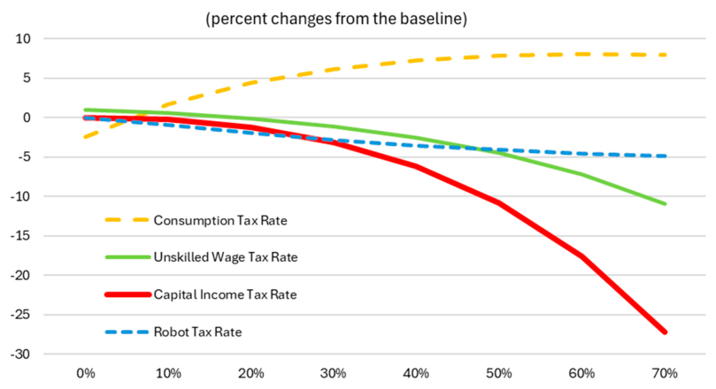
Figure A.1. Social Welfare Changes.
The optimal capital income tax rate is 2.1 percent in the absence of improvement of robot technology, which is in line with the extant literature, as Domeij (2005) found that the optimal capital income tax rate is small, in the range of -8 to 8 percent. However, the welfare gain from optimal capital taxation is nil. This is attributed to the fact that the effective capital income tax rate calibrated for the initial steady state is relatively lower than the other tax rates. If the capital income tax rate is lower than the optimal rate, the welfare loss of unskilled workers outweighs the welfare gains of capitalists and skilled workers (vice versa). As the capital income tax rate rises, the associated social welfare loss increases nonlinearly because of its adverse effect on capital accumulation (Figure A.2). The capital income tax also lowers the wage premium by reducing the demand for skilled workers, who are complementary to traditional capital (Figure A.3).
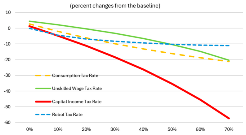
Figure A.2. Output Changes.
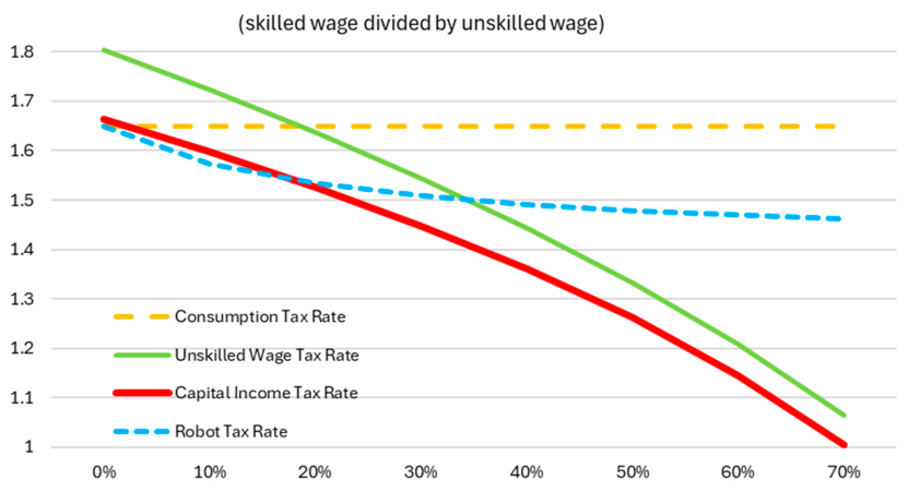
Figure A.3. Wage Premium.
In contrast, the social welfare gains from increasing the consumption tax rate are the largest among the tax reforms considered in this paper (Figure A.1). When the consumption tax rate is increased to the optimal rate of 63 percent, social welfare increases by 8 percent. This is because increased revenues from consumption tax are redistributed to unskilled workers, and their welfare gains from increased consumption surpass the welfare loss of capitalists and skilled workers. If the consumption tax rate is hiked above this optimum threshold, the welfare loss of skilled workers and capitalists outweighs the redistributive welfare gains to unskilled workers, making it not optimal. However, the consumption tax does not affect the wage premium because it is levied uniformly at the consumption stage and therefore does not alter the relative labor supply of skilled and unskilled workers (Figure A.3).
On the other hand, if the unskilled wage tax rate is reduced from the original 18.4 percent, it will gradually improve social welfare through the improvement in unskilled workers’ welfare. When the unskilled wage tax rate is reduced to the lowest zero percent, the social welfare gain becomes 0.99 percent, which is above the case of optimal capital income taxation but below the case of the optimal consumption tax rate. The changes in output in response to the unskilled wage tax are relatively smaller than those in response to the other tax instruments because it mainly affects the unskilled labor market and does not directly affect capital accumulation (Figure A.2).
Finally, introducing a robot tax lowers social welfare by generating a deadweight loss through reduced investment in automation-related capital. When the robot tax is increased to a greater percentage, the output declines become smaller than in the case of capital income taxation because substitution between automation capital and unskilled labor takes place. As a result, the share of net transfers to unskilled workers in their incomes remains relatively flat (Figure A.4).
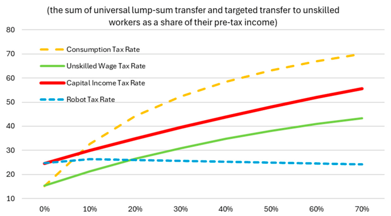
Figure A.4. Net Transfers to Unskilled Workers.
References
- Abel, A. Optimal Capital Income Taxation. NBER Working Paper 13354, 2007. [Google Scholar]
- Acemoglu, D. Harms of AI. In The Oxford Handbook of AI Governance; Bullock, Justin B., Ed.; 2023. [Google Scholar]
- Acemoglu, D.; Autor, D. Skills, Tasks, and Technologies: Implications for Employment and Earnings. Handb. Labor Econ. 2011, 4B, 1043–1171. [Google Scholar] [CrossRef]
- Acemoglu, D.; Restrepo, P. Tasks, Automation and the Rise in US Wage Inequality. Econometrica 2022, 90(5), 1973–2016. [Google Scholar] [CrossRef]
- Adachi, D. Elasticity of Substitution between Robots and Workers: Theory and Evidence from Japanese Robot Price Data. J. Monet. Econ. 2025, 152, 103782. [Google Scholar] [CrossRef]
- Afonso, O.; Sequeira, T.; Almeida, D. Technological-Knowledge and Wages: From Skill Premium to Wage Polarization. J. Econ. 2023, 140, 93–119. [Google Scholar] [CrossRef]
- Alvaredo, F.; Atkinson, A.; Piketty, T.; Saez, E. The Top 1 Percent in International and Historical Perspective. J. Econ. Perspect. 2013, 27(3), 3–20. [Google Scholar] [CrossRef]
- American Bankruptcy Institute. Study Finds That Many High-Income Workers Have Zero Savings. 2016. [Google Scholar]
- Atkinson, A.; Stiglitz, J. The Design of Tax Structure: Direct versus Indirect Taxation. J. Public Econ. 1976, 6(1–2), 55–75. [Google Scholar] [CrossRef]
- Auray, S.; Eyquem, A. On Automation, Labor Reallocation and Welfare. J. Econ. Dyn. Control 2025, 177, 105129. [Google Scholar] [CrossRef]
- Barkai, S. Declining Labor and Capital Shares. J. Financ. 2020, 75(5), 2421–2463. [Google Scholar] [CrossRef]
- Berg, A.; Bounader, L.; Gueorguiev, N.; Miyamoto, H.; Moriyama, K.; Nakatani, R.; Zanna, L. For the Benefit of All: Fiscal Policies and Equity-Efficiency Trade-offs in the Age of Automation. IMF Working Paper 2021/187, 2021. [Google Scholar]
- Berg, A.; Buffie, E.; Zanna, L. Should We Fear the Robot Revolution? (The Correct Answer is Yes). J. Monet. Econ. 2018, 97, 117–148. [Google Scholar] [CrossRef]
- Borjas, G.; Freeman, R. From Immigrants to Robots: The Changing Locus of Substitutes for Workers. Russell Sage Found. J. Soc. Sci. 2019, 5(5), 22–42. [Google Scholar] [CrossRef]
- Brezis, E.; Rubin, A. Will Automation and Robotics Lead to More Inequality? Manch. Sch. 2024, 92(3), 209–230. [Google Scholar]
- Cassas, P.; Torres, J. Automation, Automatic Capital Returns, and the Functional Income Distribution. Econ. Innov. New Technol. 2023, 32(1), 113–135. [Google Scholar]
- Cassas, P.; Torres, J. Government Size and Automation. Int. Tax. Public Financ. 2024, 31, 780–807. [Google Scholar] [CrossRef]
- Chamley, C. Optimal Taxation of Capital Income in General Equilibrium with Infinite Lives. Econometrica 1986, 54(3), 607–622. [Google Scholar] [CrossRef]
- Charalampidis, N.; Guillochon, J. Searching for Robots. Econ. Model. 2025, 152, 107260. [Google Scholar] [CrossRef]
- Charalampidis, N.; Razafitsiory, M. Automation in an Estimated Small Open Economy Model. Can. J. Econ. 2025, 58(3), 1017–1043. [Google Scholar] [CrossRef]
- Chetty, R.; Guren, A.; Manoli, D.; Weber, A. Are Micro and Macro Labor Supply Elasticities Consistent? A Review of Evidence on the Intensive and Extensive Margins. Am. Econ. Rev. 2011, 101(3), 471–475. [Google Scholar] [CrossRef]
- Costinot, A.; Werning, I. Robots, Trade, and Luddism: A Sufficient Statistic Approach to Optimal Technology Regulation. Rev. Econ. Stud. 2023, 90(5), 2261–2291. [Google Scholar]
- DeCanio, S. Robots and Humans—Complements or Substitutes? J. Macroecon. 2016, 49, 280–291. [Google Scholar] [CrossRef]
- Despard, M.; Friedline, T.; Martin-West, S. Why Do Households Lack Emergency Savings? The Role of Financial Capability. J. Fam. Econ. Issues 2020, 42, 542–557. [Google Scholar] [CrossRef]
- Diamond, P. Optimal Income Taxation: An Example with a U-Shaped Pattern of Optimal Marginal Tax Rates. Am. Econ. Rev. 1998, 88(1), 83–95. [Google Scholar]
- Dixit, A.; Stiglitz, J. Monopolistic Competition and Optimum Product Diversity. Am. Econ. Rev. 1977, 67(3), 297–308. [Google Scholar]
- Domeij, D. Optimal Capital Taxation and Labor Market Search. Rev. Econ. Dyn. 2005, 8, 623–650. [Google Scholar] [CrossRef]
- Domeij, D.; Heathcote, J. On the Distributional Effects of Reducing Capital Taxes. Int. Econ. Rev. 2004, 45(2), 523–554. [Google Scholar] [CrossRef]
- Firooz, H.; Liu, Z.; Wang, Y. Automation and the Rise of Superstar Firm. J. Monet. Econ. 2025, 151, 103733. [Google Scholar] [CrossRef]
- Ganapati, S. The Modern Wholesaler: Global Sourcing, Domestic Distribution, and Scale Economies. Am. Econ. J. Microecon. 2025, 17(1), 1–40. [Google Scholar] [CrossRef]
- Gasteiger, E.; Prettner, K. Automation, Stagnation, and the Implications of a Robot Tax. Macroecon. Dyn. 2022, 26, 218–249. [Google Scholar]
- Greenwood, J.; Hercowitz, Z.; Huffman, G. Investment, Capacity Utilization, and the Real Business Cycle. Am. Econ. Rev. 1988, 78(3), 402–417. [Google Scholar]
- Growiec, J.; Prettner, J.; Szkrobka, M. Workers’ Incentives and the Optimal Taxation of AI. Econ. Lett. 2026, 266, 113062. [Google Scholar] [CrossRef]
- Guerreiro, J.; Rebelo, S.; Teles, P. Should Robots Be Taxed? Rev. Econ. Stud. 2022, 89(1), 279–311. [Google Scholar]
- Guimarães, L.; Gil, P. Looking Ahead at the Effects of Automation in an Economy with Matching Frictions. J. Econ. Dyn. Control 2022, 144, 104538. [Google Scholar] [CrossRef]
- Havranek, T.; Horvath, R.; Irsova, Z.; Rusnak, M. Cross-Country Heterogeneity in Intertemporal Substitution. J. Int. Econ. 2015, 96, 100–118. [Google Scholar] [CrossRef]
- Hsieh, C.; Rossi-Hansberg, E. The Industrial Revolution in Services. J. Political Econ. Macroecon. 2023, 1(1), 3–42. [Google Scholar] [CrossRef]
- Jaimovich, N.; Saporta-Eksten, I.; Siu, H.; Yedid-Levi, Y. The Macroeconomics of Automation: Data, Theory, and Policy Analysis. J. Monet. Econ. 2021, 122, 1–16. [Google Scholar] [CrossRef]
- Judd, K. Redistributive Taxation in a Simple Perfect Foresight Model. J. Public Econ. 1985, 28(1), 59–83. [Google Scholar] [CrossRef]
- Judd, K. Capital-Income Taxation with Imperfect Competition. Am. Econ. Rev. 2002, 92(2), 417–421. [Google Scholar] [CrossRef]
- Korinek, A.; Stiglitz, J. NBER Working Paper 34994; Steering Technological Progress. 2026.
- Krusell, P.; Ohanian, L.; Ríos-Rull, J.; Violante, G. Capital-Skill Complementarity and Inequality: A Macroeconomic Analysis. Econometrica 2000, 68(5), 1029–1053. [Google Scholar] [CrossRef]
- Kudoh, N.; Miyamoto, H. Robots, AI, and Unemployment. J. Econ. Dyn. Control 2025, 174, 105069. [Google Scholar] [CrossRef]
- Lankisch, C.; Prettner, K.; Prskawetz, A. How Can Robots Affect Wage Inequality? Econ. Model. 2019, 81, 161–169. [Google Scholar] [CrossRef]
- Lu, C. Automation, Skill Premium, and Labor Share. B.E. J. Macroecon. 2025, 25(2), 763–798. [Google Scholar] [CrossRef]
- Moll, B.; Rachel, L.; Restrepo, P. Uneven Growth: Automation’s Impact on Income and Wealth Inequality. Econometrica 2022, 90(6), 2645–2683. [Google Scholar] [CrossRef]
- Naito, H. Re-Examination of Uniform Commodity Taxes under a Non-Linear Income Tax System and Its Implication for Production Efficiency. J. Public Econ. 1999, 71(2), 165–188. [Google Scholar] [CrossRef]
- Nakatani, R. Productivity Drivers of Infrastructure Companies: Network Industries Utilizing Economies of Scale in the Digital Era. Ann. Public Coop. Econ. 2023, 94(4), 1273–1298. [Google Scholar] [CrossRef]
- Nakatani, R. Multifactor Productivity Growth Enhancers Across Industries and Countries: Firm-Level Evidence. Eurasian Bus. Rev. 2024, 14(2), 401–446. [Google Scholar] [CrossRef]
- Prettner, K.; Strulik, H. Innovation, Automation, and Inequality: Policy Challenges in the Race Against the Machine. J. Monet. Econ. 2020, 116, 249–265. [Google Scholar] [CrossRef]
- Saez, E. Taxing the Rich More: Preliminary Evidence from the 2013 Tax Increase. Tax. Policy Econ. 2017, 31(1), 71–120. [Google Scholar] [CrossRef]
- Saez, E.; Zucman, G. The Rise of Income and Wealth Inequality in America: Evidence from Distributional Macroeconomic Accounts. J. Econ. Perspect. 2020, 34(4), 3–26. [Google Scholar] [CrossRef]
- Stiglitz, J. Pareto Efficient Taxation and Expenditures: Pre- and Re-Distribution. J. Public Econ. 2018, 162, 101–119. [Google Scholar] [CrossRef]
- Straub, L.; Werning, I. Positive Long-Run Capital Taxation: Chamley-Judd Revisited. Am. Econ. Rev. 2020, 110(1), 86–119. [Google Scholar] [CrossRef]
- Thuemmel, U. Optimal Taxation of Robots. J. Eur. Econ. Assoc. 2023, 21(3), 1154–1190. [Google Scholar]
- Tyers, R.; Zhou, Y. Automation and Inequality with Taxes and Transfers. Scott. J. Political Econ. 2023, 70, 68–100. [Google Scholar]
- Zhang, P. Automation, Wage Inequality and Implications of a Robot Tax. Int. Rev. Econ. Financ. 2019, 59, 500–509. [Google Scholar] [CrossRef]

Table 1.
Calibration.
| Parameter | Description | Value | Source or Target |
| Parameters Borrowed from the Literature | |||
| Productivity of automation technology | 0.5 | Berg et al. (2018) | |
| Elasticity of substitution between composite capital and composite labor | 0.67 | Berg et al. (2018) | |
| Elasticity of substitution between unskilled labor and automation capital | 1.9 | DeCanio (2016) | |
| Elasticity of substitution between skilled labor and capital | 0.335 | Berg et al. (2018) | |
| The inverse of intertemporal elasticity of substitution for unskilled workers | 2 | Berg et al. (2018) | |
| The inverse of intertemporal elasticity of substitution for skilled workers | 2 | Berg et al. (2018) | |
| The inverse of intertemporal elasticity of substitution for capitalists | 2 | Berg et al. (2018) | |
| The inverse of Frisch elasticity of unskilled labor supply | 2 | Chetty et al. (2011) | |
| The inverse of Frisch elasticity of skilled labor supply | 2 | Chetty et al. (2011) | |
| Discount factor | 0.94 | Berg et al. (2018) | |
| Depreciation rate of capital | 0.05 | Berg et al. (2018) | |
| Depreciation rate of robots | 0.15 | Borjas and Freeman (2019) | |
| Parameters Jointly Calibrated | |||
| Share parameter of composite input in production | 0.772 | Berg et al. (2018) | |
| Share parameter of unskilled labor in composite labor | 0.964 | Berg et al. (2018) | |
| f | Share parameter of skilled labor in composite capital | 0.092 | Berg et al. (2018) |
| Disutility of unskilled work | 9.82 | =1/3 (i.e., 8 hours) | |
| Disutility of skilled work | 31.5 | Afonso et al. (2023) | |
| Total factor productivity | 0.422 | Berg et al. (2018) | |
| Tax rate on income from skilled/unskilled labor | 0.184 | U.S. data (9.3% of GDP) | |
| Tax rate on income from capital | 0.022 | U.S. data (0.7% of GDP) | |
| Tax rate on markup | 0.104 | U.S. data (1.8% of GDP) | |
| Tax rate on consumption | 0.055 | U.S. data (4.5% of GDP) | |
| The elasticity of substitution (implied markup is 1.21) | 5.762 | Barkai (2020) | |
Table 2.
Changes in the Welfare and Economic Variables under Optimal Taxation against Different Elasticities of Substitution.
Table 2.
Changes in the Welfare and Economic Variables under Optimal Taxation against Different Elasticities of Substitution.
| Elasticity of Substitution: σ_2 | 1.9 | 2.5 | 5 | 10 | 15 | 20 |
| Optimal Capital Income Tax Rate | 3.6% | 8.5% | 22.7% | 28.1% | 29.6% | 30.2% |
| Social Welfare Gain | 0.01% | 0.28% | 6.99% | 11.36% | 12.29% | 12.66% |
| Unskilled Workers’ Welfare Gain | 0.74% | 4.75% | 29.61% | 40.50% | 42.75% | 43.59% |
| Skilled Workers’ Welfare Gain | -0.85% | -5.00% | -19.87% | -23.26% | -23.91% | -24.09% |
| Capitalists’ Welfare Gain | -1.41% | -7.84% | -28.42% | -33.08% | -34.05% | -34.33% |
| Optimal Robot Tax Rate | 0% | 0.9% | 6.1% | 8.8% | 9.6% | 10.0% |
| Social Welfare Gain | 0.00% | 0.04% | 3.78% | 6.37% | 6.87% | 7.06% |
| Unskilled Workers’ Welfare Gain | 0.00% | 1.16% | 16.93% | 23.88% | 25.11% | 25.58% |
| Skilled Workers’ Welfare Gain | 0.00% | -1.27% | -11.83% | -14.42% | -14.79% | -14.94% |
| Capitalists’ Welfare Gain | 0.00% | -2.01% | -16.81% | -20.39% | -20.95% | -21.18% |
| Optimal Unskilled Wage Tax Rate | 14.3% | 3.1% | 3.6% | 1.1% | 0% | 0% |
| Social Welfare Gain | 0.27% | 0.49% | 0.10% | 0.01% | 0.00% | 0.00% |
| Unskilled Workers’ Welfare Gain | -0.14% | -0.69% | 0.01% | 0.01% | 0.01% | 0.01% |
| Skilled Workers’ Welfare Gain | 0.77% | 1.89% | 0.21% | 0.00% | 0.00% | 0.00% |
| Capitalists’ Welfare Gain | 0.91% | 2.00% | 0.08% | -0.00% | -0.00% | -0.00% |
| Optimal Consumption Tax Rate¶ | 66.8% | 83.2% | 126.1% | 133.9% | 134.7% | 135.0% |
| Social Welfare Gain | 9.19% | 15.33% | 47.69% | 59.21% | 60.87% | 61.39% |
| Unskilled Workers’ Welfare Gain | 45.63% | 60.70% | 126.67% | 148.57% | 151.67% | 152.65% |
| Skilled Workers’ Welfare Gain | -34.02% | -38.52% | -46.24% | -47.12% | -47.18% | -47.20% |
| Capitalists’ Welfare Gain | -49.63% | -56.24% | -68.09% | -69.68% | -69.84% | -69.89% |
¶: Consumption tax rates are reported on a tax-exclusive basis, consistent with household budget constraints. For example, a tax-exclusive rate of 66.8 percent corresponds to a tax-inclusive rate of approximately 40 percent. Rates above 100 percent in the high-substitutability cases should be interpreted as model-implied restricted optima under the maintained one-instrument fiscal closure, not as literal statutory policy prescriptions.
Disclaimer/Publisher’s Note: The statements, opinions and data contained in all publications are solely those of the individual author(s) and contributor(s) and not of MDPI and/or the editor(s). MDPI and/or the editor(s) disclaim responsibility for any injury to people or property resulting from any ideas, methods, instructions or products referred to in the content. |
© 2026 by the authors. Licensee MDPI, Basel, Switzerland. This article is an open access article distributed under the terms and conditions of the Creative Commons Attribution (CC BY) license (http://creativecommons.org/licenses/by/4.0/).
Copyright: This open access article is published under a Creative Commons CC BY 4.0 license, which permit the free download, distribution, and reuse, provided that the author and preprint are cited in any reuse.