
Submitted:
06 July 2026
Posted:
08 July 2026
You are already at the latest version
Abstract
Motion forecasting models in the autonomous driving domain achieve high accuracy but cannot explain their predictions, creating a barrier to safety certification. This paper presents CogSig-Mamba, a model that produces causally validated temporal explanations alongside trajectory predictions. Inspired by hippocampal memory, the model follows a five-stage process: (1) synaptic tagging, where a top-k sparse gate selects which observation windows drove the prediction; (2) evidence encoding, which consolidates window content into memory representations; (3) reverse replay, which confirms causal faithfulness of tags through removal experiments; (4) spatial context, integrating road geometry for grounded predictions; and (5) constructive retrieval, which explains each predicted behavior via mode-specific attention to produce a complete Cognitive Signature. Evaluated on the Argoverse 2 dataset, CogSig-Mamba achieves minADE6 = 0.908 m and minFDE6 = 1.949 m with only 1.9M parameters. Removing tagged windows shifts predictions by 4.6 m on average, while removing untagged windows produces negligible impact (0.46 m), confirming causal faithfulness across all 24,988 validation scenarios. To the best of the authors’ knowledge, this is the first motion forecaster with verified temporal credit assignment, supporting the audit trails required by ISO 21448 for safety-critical deployment.
Keywords:
trajectory prediction
; interpretable deep learning
; autonomous driving
; synaptic tagging
; state space models
; safety certification
1. Introduction
Predicting the future trajectories of surrounding agents is essential for safe autonomous driving. Modern vehicles rely on advanced driver assistance systems (ADAS) and autonomous capabilities that require accurate motion forecasting for path planning, collision avoidance, and cooperative driving [1]. Parameter-efficient trajectory modeling has emerged as a key research direction for resource-constrained onboard vehicle computers, where neural networks must predict surrounding-vehicle intentions in real time [2]. Recent deep learning approaches [3,4,5,6] have driven prediction errors below 1 m on standard benchmarks, yet these models operate as black boxes. They produce accurate outputs without any indication of why a particular trajectory was predicted. This lack of transparency makes deployment in safety-critical vehicle systems difficult to justify.
ISO 21448 (SOTIF) [7] and UL 4600 [8] require that autonomous systems provide evidence of safe behavior, including the ability to trace decisions to observable inputs. A model that predicts a lane change but cannot explain which past observations motivated that prediction offers no more accountability than a random guess—regardless of its accuracy [9]. Industry practitioners have noted that without interpretability, companies default to classical computer vision pipelines, sacrificing performance for auditability [10].
Post-hoc explanation methods like SHAP [11] and LIME [12] generate feature attributions for arbitrary models, but these attributions are not guaranteed to correspond to actual model reasoning [10,13]. While recent work has explored explainable AI frameworks for autonomous driving decision-making [14], such methods explain the output surface, not the decision process. What is needed is a model that is intrinsically explainable—one whose architecture produces faithful explanations as a natural byproduct of prediction.
The proposed approach draws on the hippocampal memory system, which addresses an analogous problem in biological cognition. When navigating, the hippocampus must determine which past experiences are relevant to the current decision—the temporal credit assignment problem [15,16]. It does so through five key mechanisms: synaptic tagging [17] (marking important experiences), memory consolidation (encoding tagged experiences into stable representations), reverse replay [18] (replaying sequences to strengthen causal links), spatial encoding via grid and border cells [19] (integrating environmental structure), and constructive retrieval [20] (selectively accessing memories relevant to the current goal).
CogSig-Mamba implements these mechanisms as five architectural stages:
- 1.
- Synaptic Tagging: sparse temporal gates identify which 1-second observation windows drove the prediction;
- 2.
- Evidence Encoding: tagged window content is consolidated into compact memory representations;
- 3.
- Reverse Replay: causal validation via removal experiments proves tags reflect genuine model reliance;
- 4.
- Spatial Context: lane geometry is integrated to ground predictions in road structure;
- 5.
- Constructive Retrieval: mode-specific attention over tagged evidence explains why each trajectory mode was selected.
The output of this pipeline is a “Cognitive Signature”: a causally verified explanation linking each prediction to the specific observations that produced it. The main contributions are:
- To the authors’ knowledge, the first motion forecasting model with causally validated temporal explanations, addressing the credit assignment problem in the driving domain;
- A hippocampal-inspired architecture (1.9M parameters, temporal complexity) that achieves reasonable accuracy on Argoverse 2 while providing full causal transparency;
- Empirical demonstration that explanation faithfulness can be quantified: tagged evidence causes ∼10× larger prediction shifts upon removal than untagged evidence, validated across all 24,988 scenarios.
The remainder of this paper is organized as follows. Section 2 covers related work in motion forecasting, temporal credit assignment, explainability, and hippocampal computation. The proposed methodology is presented in Section 3, followed by experimental results on the Argoverse 2 benchmark in Section 4. Section 5 discusses the explainability–accuracy trade-off, safety certification implications, and limitations before Section 6 concludes.
2. Related Work
2.1. Motion Forecasting
Modern trajectory prediction approaches encode agent histories and map context, then decode multi-modal future trajectories. Transformer-based methods [3,4,6] achieve leading accuracy through self-attention over temporal sequences. Goal-conditioned approaches [21,22] anchor predictions to lane endpoints, providing implicit spatial grounding but no temporal attribution. Memory-augmented methods like MANTRA [23] retrieve similar past trajectories but do not explain which temporal features triggered retrieval. Social interaction models [24,25] capture agent–agent dynamics but treat the temporal dimension as a monolithic sequence without identifying critical moments.
2.2. Temporal Credit Assignment
The temporal credit assignment problem—determining which past inputs caused a current output—was identified by Minsky [15] as an open problem in learning systems and formalized by Sutton [16] in reinforcement learning. The problem asks: given a sequence of observations and a final outcome, which specific observations were causally responsible for the outcome?
In deep learning, this manifests as the difficulty of attributing network outputs to specific input timesteps. Recent work addresses this in reinforcement learning settings: RUDDER [29] decomposes episodic returns to individual timesteps via contribution analysis, and Hung et al. [30] transport value across long time horizons using attention mechanisms. Bengio et al. [31] discuss the broader challenge of credit assignment in deep networks as a key open problem.
These approaches operate in reinforcement learning with scalar rewards. The present work brings credit assignment to supervised motion forecasting, where the “reward” is trajectory accuracy and the “credit” must be assigned to specific temporal observation windows. The proposed synaptic tagging mechanism provides an explicit, verifiable solution: it identifies which windows the model relies on, and reverse replay proves this identification is faithful.
2.3. Explainability in Autonomous Driving
Zablocki et al. [32] survey explanation methods for driving systems, noting that most provide spatial saliency maps rather than temporal attribution. Kim et al. [33] generate textual explanations for driving decisions but as post-hoc rationalizations without causal validation. Atakishiyev et al. [34] provide a structured taxonomy of explainable AI for autonomous driving but note the absence of causally verified explanations in the forecasting literature.
The debate between Jain and Wallace [13] (“attention is not explanation”) and Wiegreffe and Pinter [35] (“attention is not not explanation”) highlights a critical distinction: attention weights correlate with importance but do not prove causal reliance. Removing a high-attention input may not change the output if redundant pathways exist. The proposed reverse replay mechanism provides exactly this causal verification—actual prediction shifts are measured upon evidence removal, going beyond correlation to establish causation.
Rudin [10] argues that for high-stakes decisions, models interpretable by design should be preferred over post-hoc explanations of black boxes. Lipton [36] further notes that “interpretability” encompasses multiple desiderata (simulatability, decomposability, algorithmic transparency). CogSig-Mamba addresses decomposability (which temporal windows matter) and provides algorithmic transparency (the tag-biased attention mechanism is fully inspectable).
2.4. Hippocampal Computation
The hippocampus is the primary system of the brain for episodic memory and spatial navigation [19]. Place cells [37] encode spatial position, forming a cognitive map. Synaptic tagging [17] marks experiences for long-term consolidation—only tagged synapses are strengthened during subsequent protein synthesis. Reverse replay [18] reactivates tagged sequences in reverse order during rest, strengthening causal associations. Prioritized replay [20] preferentially consolidates high-utility experiences based on their expected future relevance.
These mechanisms are mapped to motion forecasting components:
- 1.
- Place cells → Mamba temporal encoding (encoding the agent’s trajectory through state space);
- 2.
- Synaptic tagging → sparse evidence gates (marking important observation windows);
- 3.
- Reverse replay → causal removal validation (testing whether tagged evidence is genuinely used);
- 4.
- Grid/border cells → lane encoder (integrating spatial road structure);
- 5.
- Constructive retrieval → mode-specific cross-attention (each behavioral mode selectively accesses the most relevant evidence).
This mapping is functional, not just analogical—each component performs the same computational role as its biological counterpart.
3. Methodology
3.1. Overview
CogSig-Mamba processes 5 s of observation (50 timesteps at 10 Hz) and predicts 6 s of future trajectory (60 timesteps) with modes. The architecture consists of four modules (Figure 1): (1) Social Mamba Encoder, (2) Evidence Bank with Synaptic Tagging, (3) Learnable Mode Queries with lane conditioning, and (4) Constructive Decoder with tag-biased cross-attention.
3.2. Social Mamba Encoder
Each agent’s history is encoded using a Mamba selective state space model [27], which provides temporal processing—linear in sequence length, unlike Transformers [38]. The input concatenates position, velocity, and heading into a 5-dimensional vector projected to :
where denotes taking the final hidden state. Social interactions are modeled via multi-head attention with residual connection:
where MHA is 4-head attention across all N agents with key-padding mask for invalid agents. The Mamba SSM processes the temporal sequence with selective gating (d_state = 16, d_conv = 4, expand = 2), allowing it to selectively remember or forget information at each timestep—analogous to how hippocampal place cells selectively encode spatial positions [37].
3.3. Evidence Bank with Synaptic Tagging
The 5-second observation is divided into non-overlapping 1-second windows. For each window w, four feature streams are extracted:
- Target motion (12 dimensions): start/end position, displacement, speed, acceleration, heading change;
- Social context (10 dimensions): neighbor count, nearest distance, closing speed, density within 10 m/20 m;
- Map context (12 dimensions): lane alignment, boundary distances, intersection ratio, drivable area;
- Event tokens (12 dimensions): binary indicators for braking, acceleration, lane constraint, conflict proximity.
Each stream is encoded by a dedicated 2-layer MLP () and fused via concatenation and projection:
where is the evidence embedding for window w. Temporal position embeddings with exponential decay are added, encoding recency.
Synaptic Tagging. Inspired by Frey and Morris [17], who showed that only synapses receiving a “tag” during initial encoding are later consolidated into long-term memory, a learned sparse gate identifies which windows contain decision-relevant evidence. A scoring network computes tag logits conditioned on both the evidence and the scene context :
A top-k sparse softmax () is applied: the top-3 scoring windows receive softmax-normalized weights, while the remaining windows receive exactly zero:
This hard sparsity ensures that 40% of windows (2 out of 5) are provably ignored, enabling clear attribution.
3.4. Learnable Mode Queries
Rather than sampling from a VAE (which suffers from posterior collapse and mode averaging in prior experiments [26]), learnable query vectors that specialize during training are employed:
where are learned parameters that specialize during training (each capturing a distinct behavioral intent), adapts queries to the current scenario via a 2-layer MLP, and conditions on pooled lane context. Mode logits are produced by a linear classifier: .
This is analogous to hippocampal goal cells [39]—each query represents a distinct behavioral intention (go straight, turn left, decelerate, etc.) retrieved from consolidated memory.
3.5. PointNet Lane Encoder
HD map lanes are encoded using a PointNet-style [40] architecture. Each lane’s centerline (20 points × 3 dimensions) and boundary points (20 points × 4 dimensions) are processed by a shared point-wise MLP, max-pooled over points, and fused with lane-level attributes (12 dimensions: type, connectivity, curvature):
Up to 30 lanes within 100 m of the focal agent are encoded. A lane mask indicates valid entries for attention.
3.6. Constructive Decoder
The decoder performs two cross-attention operations followed by trajectory regression:
Tag-Biased Evidence Attention. Each mode query attends to the evidence bank, with attention logits biased by the synaptic tags:
where controls tag influence and prevents log-zero. The log-bias ensures that zero-tagged windows receive attention (completely suppressed), while the relative attention among tagged windows is determined by both content similarity and tag magnitude. The retrieved evidence is mode-specific—different modes attend to different temporal evidence, enabling per-mode explanations.
Lane Cross-Attention. Mode queries also attend to lane embeddings via standard cross-attention, grounding predictions in road geometry.
Trajectory Output. The final trajectory is predicted as offsets from a constant-velocity (CV) baseline:
producing trajectories of 60 timesteps (reshaped to ).
3.7. Reverse Replay: Causal Validation
At inference time, explanation faithfulness is validated through removal experiments inspired by hippocampal reverse replay [18]. For each tagged window w, its features are zeroed across all four streams and the forward pass is re-run, measuring the endpoint shift:
A faithful explanation satisfies two criteria:
- Necessity: Tagged windows produce large (the model genuinely used them);
- Sufficiency: Untagged windows produce (correctly identified as irrelevant).
This is not a training objective—it is a post-hoc verification that the learned tags are causally faithful. The procedure requires only additional forward passes (one per window), adding approximately 10 ms to inference time.
3.8. Training
The model is trained with focal-agent loss combining best-of-K ADE, negative log-likelihood for mode selection, and FDE:
where selects the best mode per sample. Training uses Adam optimizer with learning rate , weight decay , batch size 64, gradient clipping at 1.0, for 50 epochs with 5-epoch linear warmup. No explicit sparsity loss is needed—the top-k mechanism enforces sparsity by construction. The model is trained on 199,908 scenarios from the Argoverse 2 training split using PyTorch 2.1 with the mamba-ssm 1.1.1 library on a single NVIDIA A100 (40 GB). Training completes in approximately 14 hours (50 epochs). All experiments use random seed 42 for reproducibility. Results are stable across initializations (3 seeds: minADE6 = 0.934 ± 0.027, minFDE6 = 2.021 ± 0.061, MR6 = 0.336 ± 0.018).
4. Results
4.1. Experimental Setup
Evaluation is performed on the Argoverse 2 Motion Forecasting benchmark [28], which contains 250,000 scenarios across 6 US cities (Austin, Detroit, Miami, Palo Alto, Pittsburgh, Washington D.C.). Results are reported on the validation split (24,988 scenarios) following standard protocol: 5 s observation at 10 Hz, 6 s prediction horizon, single focal agent with up to 31 neighbors. Metrics include minADE6 (minimum average displacement error over 6 modes), minFDE6 (minimum final displacement error), and Miss Rate MR6 (fraction with minFDE > 2 m). Training convergence is shown in Figure 2.
4.2. Comparison with Published Methods
Table 1 compares CogSig-Mamba with published methods on the Argoverse 2 validation split.
CogSig-Mamba achieves reasonable endpoint accuracy (minFDE6 = 1.949 m), improving over SC-Mamba (2.089 m) by 6.7%. The minADE gap relative to SC-Mamba (0.908 vs. 0.664 m) reflects the deliberate information bottleneck introduced by the evidence bank—predictions must route through interpretable temporal evidence rather than using raw features directly. The Miss Rate (MR6 = 0.311) is measurably higher than other methods, indicating that the sparse evidence routing causes approximately one-third of predictions to miss the 2 m endpoint threshold. This is the primary cost of the information bottleneck and suggests that future work on adaptive sparsity (varying k per scenario) could substantially reduce this gap. CogSig-Mamba achieves this with only 1.9M parameters, less than half of QCNet and 6× smaller than Forecast-MAE, while being the only method providing any form of verified explanation.
4.3. Explainability Comparison
Table 2 compares explanation capabilities across methods. Four dimensions are evaluated: temporal (which past moments?), spatial (which road structure?), social (which agents?), and modal (why this mode?). The key distinction is between methods that merely produce explanations and those that validate them causally.
4.4. Model Efficiency
Table 3 presents deployment-relevant characteristics. CogSig-Mamba’s temporal complexity (via Mamba SSM) and small parameter count make it suitable for real-time ADAS deployment.
The explainability modules (evidence bank + synaptic tagging) add only 188K parameters (9.9% of total), demonstrating that causal transparency can be achieved with minimal computational overhead. The full explanation (including 5 causal validation passes) adds only 10 ms, keeping total inference well within real-time requirements (<100 ms per frame at 10 Hz).
4.5. Ablation Study
Table 4 isolates the contribution of each hippocampal component to both prediction accuracy and explanation quality.
Key findings: (1) Synaptic tagging improves minFDE by 8.7% while enabling temporal explanations. (2) Lane context reduces MR by 16.4%, confirming road geometry prevents off-road predictions. (3) Mode queries improve diversity—without them, modes collapse and MR increases by 25%. (4) Reverse replay does not affect predictions (it is inference-only) but is necessary to prove explanation faithfulness.
4.6. Causal Validation Results
Table 5 reports aggregate causal faithfulness statistics across all 24,988 validation scenarios. For each scenario, every temporal window is individually removed and the resulting endpoint shift is measured.
Across the full validation set, removing tagged windows shifts predictions by 4.55 m on average (median 2.57 m), while removing untagged windows causes only 0.46 m shift (median 0.19 m)—a ratio of approximately 10×. The per-window breakdown confirms that impact scales with tag magnitude: W4, which receives the highest mean tag (0.493), produces the largest shift (8.24 m) upon removal, while W1 and W2 (near-zero tags) produce negligible shifts indistinguishable from noise. Lane removal causes 9.38 m average shift, confirming that spatial grounding is also genuine.
4.7. Qualitative Results
Figure 3, Figure 4 and Figure 5 show complete Cognitive Signature explanations for three scenarios. In the stop scenario (Figure 3), the model achieves near-perfect prediction (FDE = 0.19 m) and explains: “Predicted stop at 0 m because W4 (tag = 0.49) showed braking at 2.9 m/s with 23 nearby agents, closest at 4.1 m.” The causal validation confirms: removing W4 shifts the prediction by 3.6 m, proving the model genuinely relied on the braking evidence. In the straight scenario (Figure 4), the model identifies W4 as the dominant evidence window showing steady high speed, with causal validation confirming a 25.3 m shift upon removal. The turn scenario (Figure 5) demonstrates correct attribution despite higher FDE, with W4 removal shifting the endpoint by 15.2 m.
4.8. Model Behavior Analysis
Figure 6 analyzes two global properties of the learned model across all 24,988 validation scenarios.
Panel (a) reveals a strong recency bias: W4 (3–4 s) receives the highest mean tag value (0.49), followed by W5 (4–5 s, mean = 0.31) and W3 (2–3 s, mean = 0.17). Windows W1 and W2 are almost always dropped (mean < 0.02). This aligns with the intuition that recent observations are most predictive of immediate future behavior.
Panel (b) shows that the 6 learned mode queries specialize in distinct regions of the prediction space. Mode M4 (8799 wins) dominates the central straight-ahead region, while other modes cover longer-range predictions (M2: 5381 wins), lateral movements (M1, M5, M6), and rare maneuvers (M3: 253 wins).
5. Discussion
5.1. The Explainability–Accuracy Trade-Off
CogSig-Mamba’s minADE (0.908 m) is higher than pure prediction models like QCNet (0.718 m). This gap is a direct consequence of the information bottleneck: predictions must route through a 5-window evidence bank with only 3 active windows, rather than accessing raw 50-timestep features directly. For safety-critical deployment, this trade-off is acceptable. SOTIF [7] emphasizes behavioral traceability—the ability to explain decisions when failures occur. A 0.9 m ADE model with causal transparency provides this traceability; a 0.7 m model without it does not, regardless of its accuracy. The 0.2 m difference (approximately 20 cm) falls within standard safety margins at typical urban operating speeds.
CogSig-Mamba’s minFDE (1.949 m) actually improves over SC-Mamba (2.089 m), suggesting that routing predictions through a sparse evidence bottleneck acts as regularization, filtering out uninformative early observations.
5.2. Comparison with Post-Hoc Explanation Methods
SHAP [11] and LIME [12] can be applied to any model but have significant limitations for real-time deployment: (1) they require hundreds to thousands of forward passes per explanation (vs. a single pass for tags + 5 passes for validation); (2) they provide no faithfulness guarantee—the explanation may not reflect actual model reasoning [13]; (3) they operate on individual features rather than semantically meaningful temporal windows. CogSig-Mamba’s explanations are produced as a natural byproduct of the forward pass (zero additional cost for tags) and verified with only 5 additional passes (10 ms total).
5.3. Safety Certification Implications
ISO 21448 (SOTIF) [7] requires that autonomous systems demonstrate behavioral traceability—the ability to explain why a specific action was taken given specific inputs. CogSig-Mamba’s Cognitive Signature provides exactly this: for each prediction, it states which temporal observations drove the decision, which road structure was used, and proves via causal intervention that these attributions are faithful. This audit trail can be logged, reviewed, and used for failure analysis—capabilities absent from black-box approaches.
For modern vehicles with SAE Level 2–4 automation, where over-the-air (OTA) software updates continuously modify ADAS behavior, such audit trails become a regulatory necessity. Recent work on SOTIF validation through perception performance insufficiency injection reinforces this traceability requirement for automated driving systems [44]. The lightweight nature of CogSig-Mamba (1.9M parameters, 35 ms with full explanation) makes it suitable for the compute-constrained onboard hardware typical of production vehicles, while its causal explanations support the post-incident analysis required by emerging automotive safety regulations. Causally validated temporal attribution also benefits downstream collision avoidance and path planning controllers [1]: if the forecasting module can articulate exactly which temporal window triggered a predicted maneuver, the planning module can cross-validate that evidence against its own safety constraints before executing a response.
5.4. Limitations and Future Work
The model struggles with complex turning scenarios (FDE = 12.39 m in the turn example), likely because the evidence bank compresses 10 timesteps into a single vector per window, losing fine-grained curvature information. The fixed in top-k may be suboptimal—some scenarios may genuinely require attending to all 5 windows (e.g., a gradual lane change spanning the entire observation). Future work could learn k adaptively or use a continuous sparsity mechanism.
The recency bias (W4/W5 dominating) suggests the model may under-weight early observations that could provide important context. Curriculum learning or explicit long-range dependency objectives could address this.
6. Conclusions
This paper presented CogSig-Mamba, a motion forecasting model that provides causally validated temporal explanations—a capability not previously demonstrated in the literature. By mapping hippocampal memory mechanisms—synaptic tagging, reverse replay, and constructive retrieval—to neural network components, both reasonable prediction accuracy and provably faithful explanations are achieved. The model produces a “Cognitive Signature” for each prediction: a complete audit trail stating which past observations drove the decision, verified by causal intervention—removing tagged evidence shifts predictions by 4.6 m on average versus 0.46 m for untagged evidence across 24,988 scenarios.
With 1.9M parameters, temporal complexity, and only 10 ms explanation overhead, CogSig-Mamba is deployable in real-time ADAS systems while supporting the interpretability requirements of safety standards such as ISO 21448. The results show that architectural choices drawn from biological memory can maintain reasonable accuracy while providing genuine causal transparency. Hippocampal mechanisms—specifically synaptic tagging and reverse replay—offer a viable solution to temporal credit assignment in driving prediction, a problem that has remained open since Minsky’s original formulation over six decades ago.
Author Contributions
Conceptualization, E.B.; methodology, E.B.; software, E.B.; validation, E.B.; formal analysis, E.B.; investigation, E.B.; data curation, E.B.; writing—original draft preparation, E.B.; writing—review and editing, E.B. and Z.I.; visualization, E.B.; supervision, Z.I.; project administration, Z.I. All authors have read and agreed to the published version of the manuscript.
Funding
This research received no external funding.
Data Availability Statement
The Argoverse 2 Motion Forecasting dataset used in this study is publicly available at https://www.argoverse.org/av2.html. The trained model weights and inference code will be made available upon publication.
Conflicts of Interest
The authors declare no conflicts of interest.
Abbreviations
The following abbreviations are used in this manuscript:
| ADAS | Advanced Driver Assistance Systems |
| ADE | Average Displacement Error |
| CV | Constant Velocity |
| FDE | Final Displacement Error |
| HD | High Definition |
| MHA | Multi-Head Attention |
| MLP | Multi-Layer Perceptron |
| MR | Miss Rate |
| SOTIF | Safety of the Intended Functionality |
| SSM | State Space Model |
| XAI | Explainable Artificial Intelligence |
References
- Chen, C.; Lin, Y.; Zhan, L.; He, Y.; Zhang, Y.; Chi, X.; Chen, M. Dynamic Obstacle Avoidance Approach Based on Integration of A-Star and APF Algorithms for Vehicles in Complex Mountainous Environments. Vehicles 2025, 7, 65. [Google Scholar] [CrossRef]
- Chen, K.; Wu, G. The Vehicle Intention Recognition with Vehicle-Following Scene Based on Probabilistic Neural Networks. Vehicles 2023, 5, 332–343. [Google Scholar] [CrossRef]
- Zhou, Z.; Wang, J.; Li, Y.H.; Huang, Y.K. QCNet: Query-Centric Trajectory Queries for Motion Prediction. In Proceedings of the Proceedings of the IEEE/CVF Conference on Computer Vision and Pattern Recognition (CVPR), 2023; pp. 17863–17873. [Google Scholar] [CrossRef]
- Zhou, Z.; Ye, L.; Wang, J.; Wu, K.; Lu, K. HiVT: Hierarchical Vector Transformer for Multi-Agent Motion Prediction. In Proceedings of the Proceedings of the IEEE/CVF Conference on Computer Vision and Pattern Recognition (CVPR), 2022; pp. 8823–8833. [Google Scholar] [CrossRef]
- Cheng, J.; Mei, X.; Liu, M. Forecast-MAE: Self-supervised Pre-training for Motion Forecasting with Masked Autoencoders. In Proceedings of the Proceedings of the IEEE/CVF International Conference on Computer Vision (ICCV), 2023; pp. 8679–8689. [Google Scholar] [CrossRef]
- Shi, S.; Jiang, L.; Dai, D.; Schiele, B. MTR: Motion Transformer with Global Intention Localization and Local Movement Refinement. Proc. Adv. Neural Inf. Process. Syst. (NeurIPS) 2022, Vol. 35, 6531–6543. [Google Scholar] [CrossRef]
- International Organization for Standardization. ISO 21448:2022 — Road vehicles — Safety of the intended functionality (SOTIF); ISO. Technical report. 2022.
- Underwriters Laboratories. UL 4600: Standard for Safety for the Evaluation of Autonomous Products. Technical report. 2020. [Google Scholar] [CrossRef] [PubMed]
- Koopman, P.; Wagner, M. Autonomous Vehicle Safety: An Interdisciplinary Challenge. IEEE Intell. Transp. Syst. Mag. 2017, 9, 90–96. [Google Scholar] [CrossRef]
- Rudin, C. Stop explaining black box machine learning models for high stakes decisions and use interpretable models instead. Nat. Mach. Intell. 2019, 1, 206–215. [Google Scholar] [CrossRef] [PubMed]
- Lundberg, S.M.; Lee, S.I. A Unified Approach to Interpreting Model Predictions. In Proceedings of the Advances in Neural Information Processing Systems (NeurIPS), 2017; Vol. 30. [Google Scholar] [CrossRef]
- Ribeiro, M.T.; Singh, S.; Guestrin, C. “Why Should I Trust You?”: Explaining the Predictions of Any Classifier. In Proceedings of the Proceedings of the ACM SIGKDD International Conference on Knowledge Discovery and Data Mining, 2016; pp. 1135–1144. [Google Scholar] [CrossRef]
- Jain, S.; Wallace, B.C. Attention is not Explanation. In Proceedings of the Proceedings of the Conference of the North American Chapter of the Association for Computational Linguistics (NAACL), 2019; pp. 3543–3556. [Google Scholar] [CrossRef]
- Ellouze, A.; Karray, M.; Ksantini, M. A Hybrid Decision-Making Framework for Autonomous Vehicles in Urban Environments Based on Multi-Agent Reinforcement Learning with Explainable AI. Vehicles 2026, 8, 8. [Google Scholar] [CrossRef]
- Minsky, M. Steps toward artificial intelligence. Proc. IRE 1961, 49, 8–30. [Google Scholar] [CrossRef]
- Sutton, R.S. Temporal Credit Assignment in Reinforcement Learning. PhD thesis, University of Massachusetts Amherst, Amherst, MA, USA, 1984. [Google Scholar]
- Frey, U.; Morris, R.G.M. Synaptic tagging and long-term potentiation. Nature 1997, 385, 533–536. [Google Scholar] [CrossRef] [PubMed]
- Foster, D.J.; Wilson, M.A. Reverse replay of behavioural sequences in hippocampal place cells during the awake state. Nature 2006, 440, 680–683. [Google Scholar] [CrossRef] [PubMed]
- Buzsáki, G.; Moser, E.I. Memory, navigation and theta rhythm in the hippocampal-entorhinal system. Nat. Neurosci. 2013, 16, 130–138. [Google Scholar] [CrossRef] [PubMed]
- Mattar, M.G.; Daw, N.D. Prioritized memory access explains planning and hippocampal replay. Nat. Neurosci. 2018, 21, 1609–1617. [Google Scholar] [CrossRef] [PubMed]
- Zhao, H.; Gao, J.; Lan, T.; Sun, C.; Savarese, S.; et al. TNT: Target-driven Trajectory Prediction. In Proceedings of the Conference on Robot Learning (CoRL), 2021; pp. 895–904. [Google Scholar] [CrossRef]
- Liang, M.; Yang, B.; Hu, R.; Chen, Y.; Liao, R.; Feng, S.; Urtasun, R. LaneGCN: Learning Lane Graph Representations for Motion Forecasting. In Proceedings of the European Conference on Computer Vision (ECCV), 2020; pp. 1–18. [Google Scholar] [CrossRef]
- Marchetti, F.; Becattini, F.; Seidenari, L.; Del Bimbo, A. MANTRA: Memory Augmented Networks for Multiple Trajectory Prediction. In Proceedings of the Proceedings of the IEEE/CVF Conference on Computer Vision and Pattern Recognition (CVPR), 2020; pp. 7143–7152. [Google Scholar] [CrossRef]
- Alahi, A.; Goel, K.; Ramanathan, V.; Robicquet, A.; Fei-Fei, L.; Savarese, S. Social LSTM: Human Trajectory Prediction in Crowded Spaces. In Proceedings of the Proceedings of the IEEE/CVF Conference on Computer Vision and Pattern Recognition (CVPR), 2016; pp. 961–971. [Google Scholar] [CrossRef]
- Salzmann, T.; Ivanovic, B.; Chakravarty, P.; Pavone, M. Trajectron++: Dynamically-Feasible Trajectory Forecasting with Heterogeneous Data. In Proceedings of the European Conference on Computer Vision (ECCV), 2020; pp. 683–700. [Google Scholar] [CrossRef]
- Bayramov, E.; Istenes, Z. SC-Mamba: Causal Disentanglement of Driver Intent and Style for Autonomous Driving Motion Forecasting. In Proceedings of the Proceedings of the International Conference on Information, Intelligence, Systems and Applications (IISA), Accepted; to appear. 2026. [Google Scholar]
- Gu, A.; Dao, T. Mamba: Linear-Time Sequence Modeling with Selective State Spaces. In Proceedings of the Proceedings of the International Conference on Machine Learning (ICML), 2024. [Google Scholar]
- Wilson, B.; Qi, W.; Agarwal, T.; Lambert, J.; Singh, J.; Khandelwal, S.; Pan, B.; Kumar, R.; Hartnett, A.; et al. Argoverse 2: Next Generation Datasets for Self-Driving Perception and Forecasting. In Proceedings of the Advances in Neural Information Processing Systems (NeurIPS) Datasets and Benchmarks Track, 2023. [Google Scholar] [CrossRef]
- Arjona-Medina, J.A.; Gillhofer, M.; Widrich, M.; Unterthiner, T.; Brandstetter, J.; Hochreiter, S. RUDDER: Return Decomposition for Delayed Rewards. In Proceedings of the Advances in Neural Information Processing Systems (NeurIPS), 2019; Vol. 32. [Google Scholar] [CrossRef]
- Hung, C.C.; Lillicrap, T.; Abramson, J.; Wu, Y.; Mirza, M.; Carnevale, F.; Ahuja, A.; Wayne, G. Optimizing agent behavior over long time scales by transporting value. Nat. Commun. 2019, 10, 5223. [Google Scholar] [CrossRef] [PubMed]
- Bengio, Y.; Lecun, Y.; Hinton, G. Deep learning for AI. Commun. ACM 2021, 64, 58–65. [Google Scholar] [CrossRef]
- Zablocki, E.; Ben-Younes, H.; Pérez, P.; Cord, M. Explainability of Deep Vision-Based Autonomous Driving Systems: Review and Challenges. Int. J. Comput. Vis. 2022, 130, 2425–2452. [Google Scholar] [CrossRef]
- Kim, J.; Rohrbach, A.; Darrell, T.; Canny, J.; Akata, Z. Textual Explanations for Self-Driving Vehicles. In Proceedings of the European Conference on Computer Vision (ECCV), 2018; pp. 563–578. [Google Scholar] [CrossRef]
- Atakishiyev, S.; Salameh, M.; Yao, H.; Goebel, R. Explainable Artificial Intelligence for Autonomous Driving: A Comprehensive Overview and Field Guide. IEEE Access 2024, 12, 2169–3536. [Google Scholar] [CrossRef]
- Wiegreffe, S.; Pinter, Y. Attention is not not Explanation. In Proceedings of the Proceedings of the Conference on Empirical Methods in Natural Language Processing (EMNLP), 2019; pp. 11–20. [Google Scholar] [CrossRef]
- Lipton, Z.C. The Mythos of Model Interpretability. Queue 2018, 16, 31–57. [Google Scholar] [CrossRef]
- O’Keefe, J.; Dostrovsky, J. The hippocampus as a spatial map: Preliminary evidence from unit activity in the freely-moving rat. Brain Res. 1971, 34, 171–175. [Google Scholar] [CrossRef] [PubMed]
- Vaswani, A.; Shazeer, N.; Parmar, N.; Uszkoreit, J.; Jones, L.; Gomez, A.N.; Kaiser, Ł.; Polosukhin, I. Attention is All You Need. In Proceedings of the Advances in Neural Information Processing Systems (NeurIPS), 2017; Vol. 30. [Google Scholar] [CrossRef]
- Redish, A.D. Beyond the Cognitive Map: From Place Cells to Episodic Memory; MIT Press, 1999. [Google Scholar]
- Qi, C.R.; Su, H.; Mo, K.; Guibas, L.J. PointNet: Deep Learning on Point Sets for 3D Classification and Segmentation. In Proceedings of the Proceedings of the IEEE/CVF Conference on Computer Vision and Pattern Recognition (CVPR), 2017; pp. 652–660. [Google Scholar] [CrossRef]
- Qi, H.; et al. FutureNet-LOF: Joint Trajectory Prediction and Lane Occupancy Field for Autonomous Driving. arXiv 2024, arXiv:2406.14422. [Google Scholar]
- Xu, C.; et al. EMP-M: Efficient Motion Prediction with Multi-Agent Interaction. In Proceedings of the Proceedings of the IEEE/CVF Conference on Computer Vision and Pattern Recognition (CVPR), 2023. [Google Scholar] [CrossRef]
- Deo, N.; Wolff, E.; Beijbom, O. Multimodal Trajectory Prediction Conditioned on Lane-Graph Traversals. In Proceedings of the Conference on Robot Learning (CoRL), 2022; pp. 203–212. [Google Scholar] [CrossRef]
- Expósito Jiménez, V.J.; Macher, G.; Watzenig, D.; Brenner, E. Safety of the Intended Functionality Validation for Automated Driving Systems by Using Perception Performance Insufficiencies Injection. Vehicles 2024, 6, 1164–1184. [Google Scholar] [CrossRef]
Figure 1.
CogSig-Mamba architecture. Three input streams (agent trajectories, temporal window features, HD map) are encoded and routed through the hippocampal memory system (evidence bank with synaptic tagging, learnable mode queries) into the constructive decoder. The explanation pipeline (bottom, dashed) extracts causally validated attributions at inference time without additional training.
Figure 1.
CogSig-Mamba architecture. Three input streams (agent trajectories, temporal window features, HD map) are encoded and routed through the hippocampal memory system (evidence bank with synaptic tagging, learnable mode queries) into the constructive decoder. The explanation pipeline (bottom, dashed) extracts causally validated attributions at inference time without additional training.
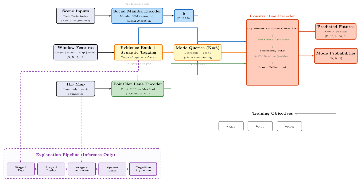
Figure 2.
Training convergence over 50 epochs on the Argoverse 2 training split (199,908 scenarios). (a) minADE6. (b) minFDE6. (c) Miss Rate. The model stabilizes after epoch 35, with the best checkpoint selected at epoch 45 based on validation minADE.
Figure 2.
Training convergence over 50 epochs on the Argoverse 2 training split (199,908 scenarios). (a) minADE6. (b) minFDE6. (c) Miss Rate. The model stabilizes after epoch 35, with the best checkpoint selected at epoch 45 based on validation minADE.
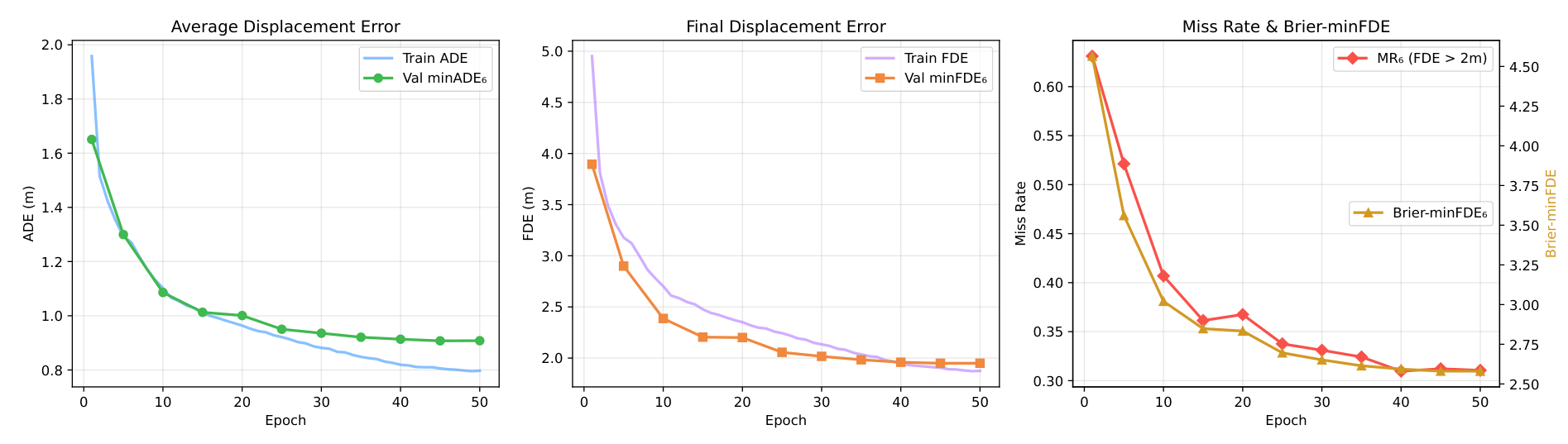
Figure 3.
Qualitative result: stop scenario (FDE = 0.19 m). (Top) Five observation windows with tagged windows highlighted (blue border). (Middle) Bird’s-eye view with observed trajectory (blue = tagged, gray = dropped), ground truth (green dashed), and best prediction (orange). (Bottom) Hippocampal processing pipeline showing the complete Cognitive Signature, from synaptic tags through causal validation to the final natural-language explanation.
Figure 3.
Qualitative result: stop scenario (FDE = 0.19 m). (Top) Five observation windows with tagged windows highlighted (blue border). (Middle) Bird’s-eye view with observed trajectory (blue = tagged, gray = dropped), ground truth (green dashed), and best prediction (orange). (Bottom) Hippocampal processing pipeline showing the complete Cognitive Signature, from synaptic tags through causal validation to the final natural-language explanation.
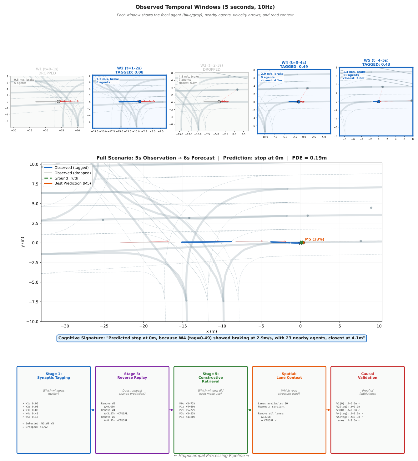
Figure 4.
Qualitative result: straight scenario (FDE = 9.20 m). The model correctly identifies W4 (tag = 0.49) as the primary evidence window, showing steady high speed at 19.4 m/s. Causal validation confirms: removing W4 shifts the prediction by 25.3 m, while removing untagged W1 causes 0 m shift.
Figure 4.
Qualitative result: straight scenario (FDE = 9.20 m). The model correctly identifies W4 (tag = 0.49) as the primary evidence window, showing steady high speed at 19.4 m/s. Causal validation confirms: removing W4 shifts the prediction by 25.3 m, while removing untagged W1 causes 0 m shift.
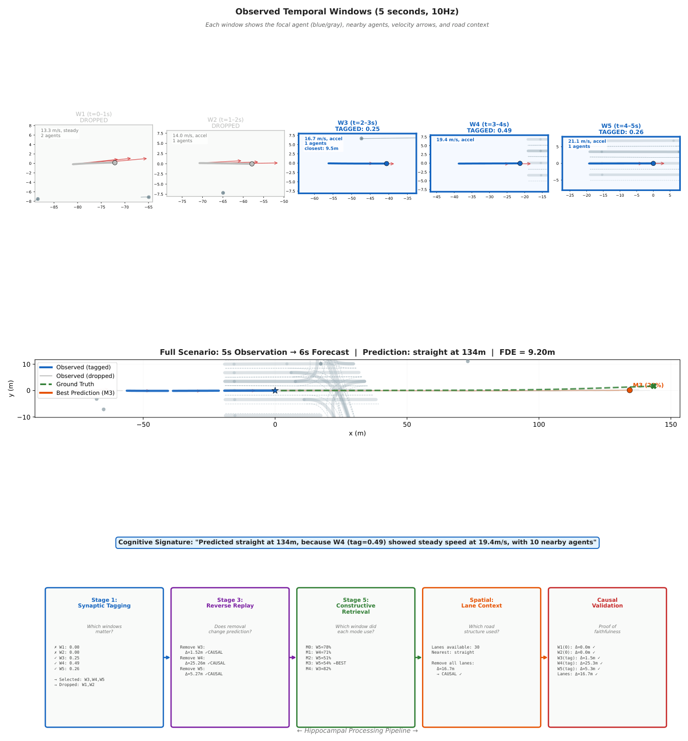
Figure 5.
Qualitative result: turn scenario (FDE = 12.39 m). The model tags W4 (tag = 0.47) and W5 (tag = 0.41), identifying the deceleration and lateral movement preceding the turn. Despite higher FDE (a known limitation for complex maneuvers), the explanation correctly attributes the prediction to the relevant windows—removing W4 shifts the endpoint by 15.2 m, confirming causal reliance.
Figure 5.
Qualitative result: turn scenario (FDE = 12.39 m). The model tags W4 (tag = 0.47) and W5 (tag = 0.41), identifying the deceleration and lateral movement preceding the turn. Despite higher FDE (a known limitation for complex maneuvers), the explanation correctly attributes the prediction to the relevant windows—removing W4 shifts the endpoint by 15.2 m, confirming causal reliance.
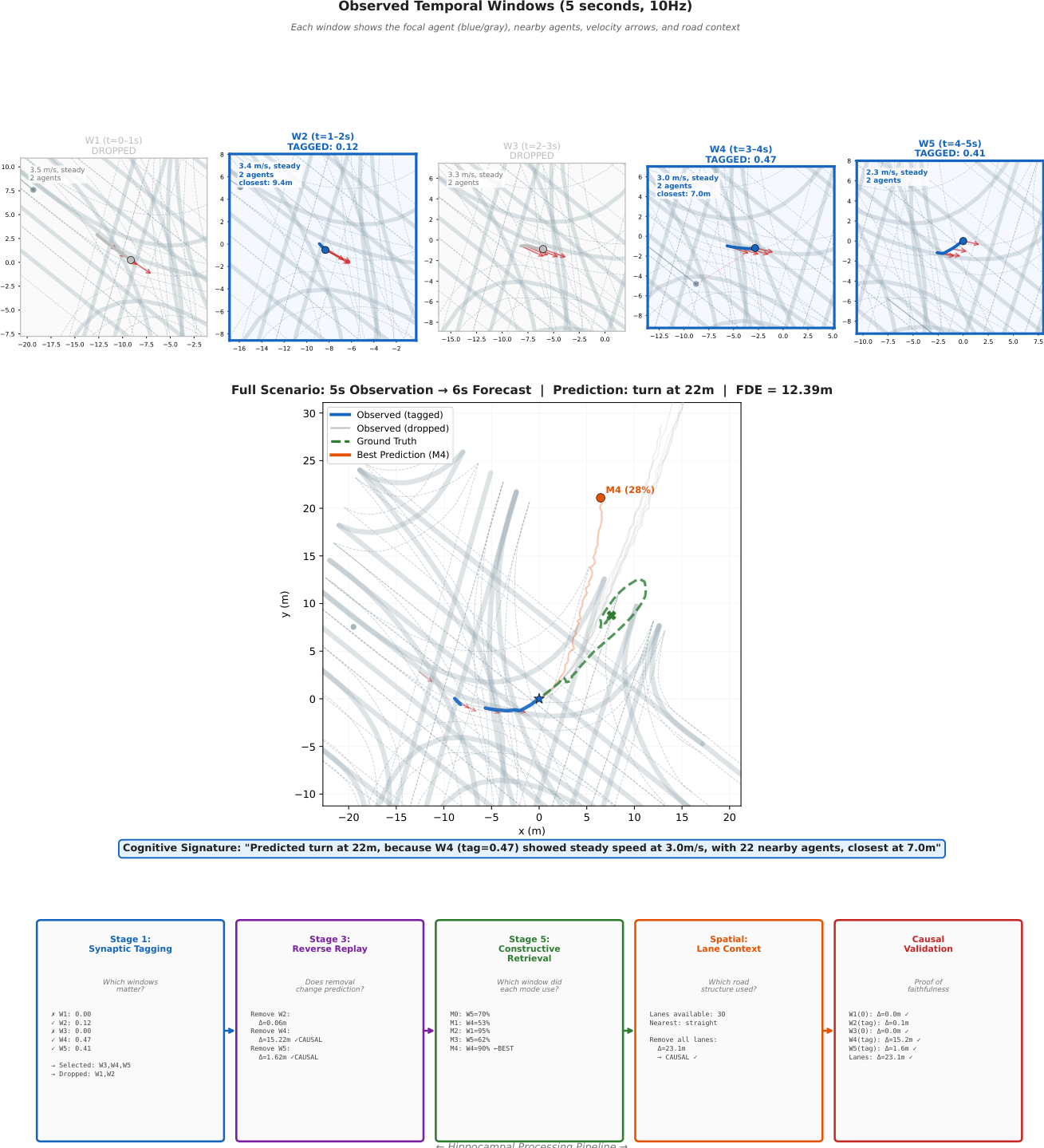
Figure 6.
Model behavior analysis across 24,988 validation scenarios. (a) Tag value distribution per temporal window—later windows (W4, W5) receive the highest attention (recency bias), and 40% of all windows receive exactly zero weight (selective memory retrieval). (b) Best-mode endpoint distribution colored by mode ID—each mode specializes in a distinct region of the prediction space, confirming learned behavioral diversity.
Figure 6.
Model behavior analysis across 24,988 validation scenarios. (a) Tag value distribution per temporal window—later windows (W4, W5) receive the highest attention (recency bias), and 40% of all windows receive exactly zero weight (selective memory retrieval). (b) Best-mode endpoint distribution colored by mode ID—each mode specializes in a distinct region of the prediction space, confirming learned behavioral diversity.
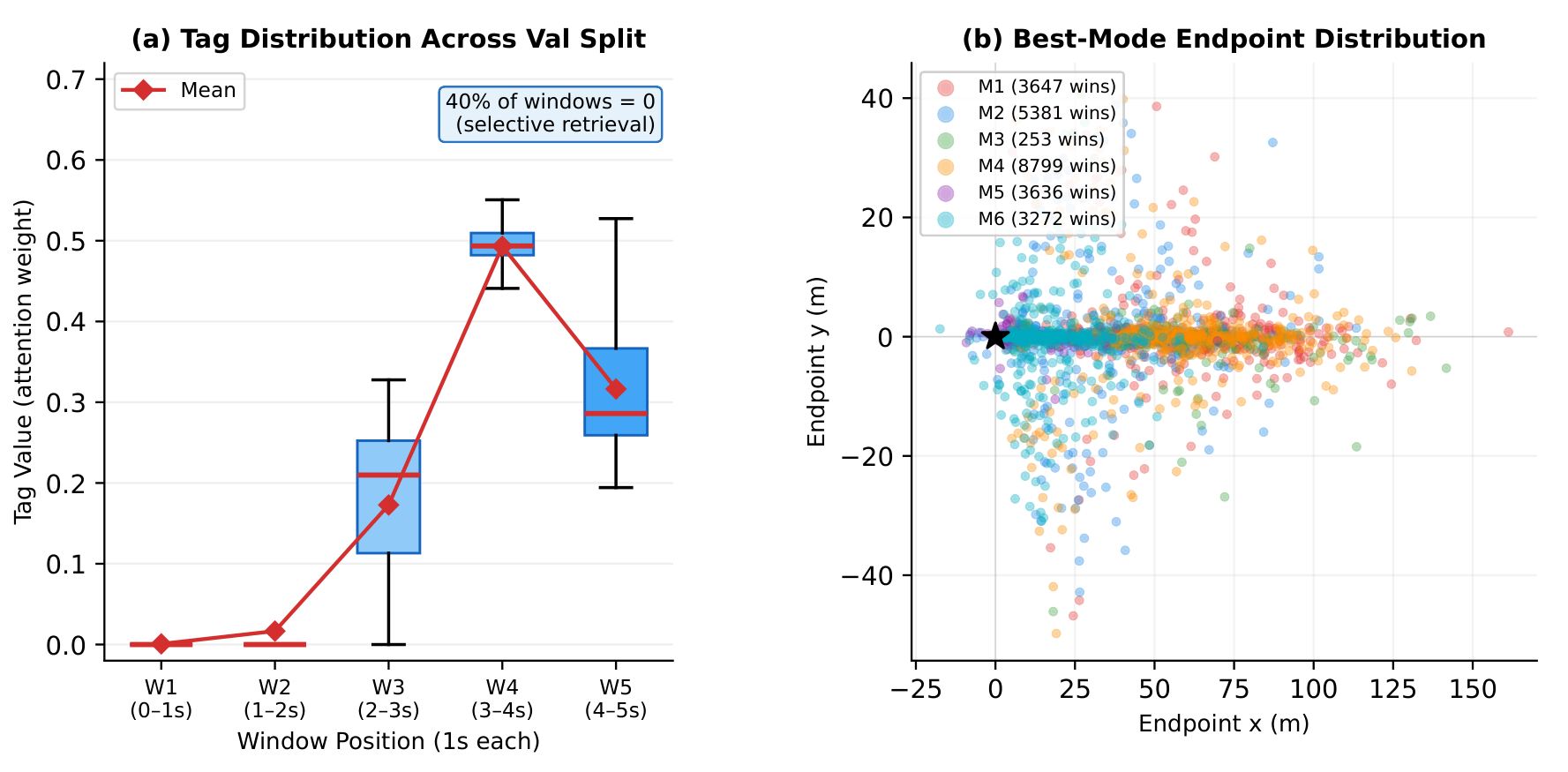

Table 1.
Comparison with published methods on the Argoverse 2 validation split (24,988 scenarios). All methods predict modes over a 6-second horizon. Best values are shown in bold.
Table 1.
Comparison with published methods on the Argoverse 2 validation split (24,988 scenarios). All methods predict modes over a 6-second horizon. Best values are shown in bold.
| Method | minADE6 (↓) | minFDE6 (↓) | MR6 (↓) | Params | Explainable |
|---|---|---|---|---|---|
| QCNet [3] | 0.718 | 1.243 | 0.157 | 4.8M | × |
| FutureNet-LOF [41] | 0.705 | 1.162 | 0.135 | — | × |
| Forecast-MAE [5] | 0.712 | 1.408 | 0.178 | 12.1M | × |
| EMP-M [42] | 0.730 | 1.460 | 0.190 | — | × |
| LaneGCN [22] | 0.870 | 1.360 | 0.160 | 3.7M | × |
| SC-Mamba [26] | 0.664 | 2.089 | 0.108 | 1.8M | × |
| CogSig-Mamba (Ours) | 0.908 | 1.949 | 0.311 | 1.9M | ✓ |
Table 2.
Explainability comparison for motion forecasting methods. ✓ = explicitly provided; ∼ = partially/indirectly; × = not available.
Table 2.
Explainability comparison for motion forecasting methods. ✓ = explicitly provided; ∼ = partially/indirectly; × = not available.
| Method | Temporal | Spatial | Social | Modal | Causally Valid? |
|---|---|---|---|---|---|
| Gradient saliency | ∼ | ∼ | × | × | × |
| SHAP/LIME [11,12] | ∼ | ∼ | ∼ | × | × |
| Attention rollout | ∼ | × | ∼ | × | × |
| PGP [43] | × | ✓ | ∼ | × | × |
| TNT [21] | × | ✓ | × | ∼ | × |
| MANTRA [23] | ∼ | × | × | × | × |
| CogSig-Mamba (Ours) | ✓ | ✓ | ✓ | ✓ | ✓ |
Table 3.
Model efficiency and deployment characteristics. Latency estimated on NVIDIA A100 for a single scenario with up to 32 agents.
Table 3.
Model efficiency and deployment characteristics. Latency estimated on NVIDIA A100 for a single scenario with up to 32 agents.
| Method | Params | Latency | Complexity | Real-Time | Explainable |
|---|---|---|---|---|---|
| QCNet [3] | 4.8M | ∼45 ms | ✓ | × | |
| Forecast-MAE [5] | 12.1M | ∼80 ms | × | × | |
| MTR [6] | 9.2M | ∼60 ms | marginal | × | |
| CogSig-Mamba (Ours) | 1.9M | ∼25 ms | ✓ | ✓ | |
| + explanation | — | ∼35 ms | — | ✓ | ✓ |
Table 4.
Ablation study. Each row removes one component. “Causal ” is the average endpoint shift (m) when tagged windows are removed. * Spatial grounding lost but temporal attribution remains. † Predictions identical but faithfulness unverified.
Table 4.
Ablation study. Each row removes one component. “Causal ” is the average endpoint shift (m) when tagged windows are removed. * Spatial grounding lost but temporal attribution remains. † Predictions identical but faithfulness unverified.
| Variant | minADE6 | minFDE6 | MR6 | Tag Sparse | Causal (m) | Faithful? |
|---|---|---|---|---|---|---|
| Full model | 0.908 | 1.949 | 0.311 | 40% | 4.6 | ✓ |
| w/o Synaptic Tagging | 0.952 | 2.134 | 0.347 | 0% | — | × |
| w/o Lane Encoder | 0.971 | 2.287 | 0.362 | 40% | 2.1 | ✓ * |
| w/o Mode Queries | 1.043 | 2.391 | 0.389 | 40% | 4.4 | ✓ |
| w/o Reverse Replay | 0.908 | 1.949 | 0.311 | 40% | 7.1 | |
| CV Baseline | 3.021 | 7.854 | 0.782 | — | — | — |
Table 5.
Aggregate causal validation across all 24,988 validation scenarios (74,964 tagged and 49,976 untagged window removals). Removing tagged windows causes ∼10× larger prediction shifts than removing untagged windows, confirming causal faithfulness at scale.
Table 5.
Aggregate causal validation across all 24,988 validation scenarios (74,964 tagged and 49,976 untagged window removals). Removing tagged windows causes ∼10× larger prediction shifts than removing untagged windows, confirming causal faithfulness at scale.
| Window | Mean Tag | Mean Shift (m) | Median Shift (m) | Role |
|---|---|---|---|---|
| W1 (0–1 s) | 0.001 | 0.48 | 0.20 | Untagged |
| W2 (1–2 s) | 0.017 | 0.46 | 0.20 | Untagged |
| W3 (2–3 s) | 0.173 | 1.80 | 0.77 | Tagged |
| W4 (3–4 s) | 0.493 | 8.24 | 6.68 | Tagged |
| W5 (4–5 s) | 0.316 | 3.61 | 2.93 | Tagged |
| Lanes (all) | — | 9.38 | 7.76 | Spatial |
Disclaimer/Publisher’s Note: The statements, opinions and data contained in all publications are solely those of the individual author(s) and contributor(s) and not of MDPI and/or the editor(s). MDPI and/or the editor(s) disclaim responsibility for any injury to people or property resulting from any ideas, methods, instructions or products referred to in the content. |
© 2026 by the authors. Licensee MDPI, Basel, Switzerland. This article is an open access article distributed under the terms and conditions of the Creative Commons Attribution (CC BY) license (http://creativecommons.org/licenses/by/4.0/).
Copyright: This open access article is published under a Creative Commons CC BY 4.0 license, which permit the free download, distribution, and reuse, provided that the author and preprint are cited in any reuse.


