Explainable Machine Learning and Necessary Condition Analysis for Product Sales Forecasting in Retail

Marcin Nowak; Paweł Kościelniak

doi:10.20944/preprints202607.0593.v1

Submitted:

07 July 2026

Posted:

08 July 2026

You are already at the latest version

Abstract

Sales forecasting in retail and e-commerce-related environments supports key decisions concerning inventory management, promotion planning, pricing policy, and sales strategy optimization. The aim of this article is to develop a predictive framework for product sales forecasting using machine learning regression algorithms, Explainable AI methods, and Necessary Condition Analysis. The study employed the Walmart M5 retail sales forecasting dataset, including daily product-level sales observations with calendar, product hierarchy, event-related, price-related, and historical demand features. The benchmark included a naive weekly model, Ridge regression, Random Forest, Extra Trees, XGBoost, and LightGBM. Predictive performance was evaluated using RMSE, MAE, R², WMAPE, and RMSSE under rolling-origin validation and on a final 28-day test period. The best-performing model was interpreted using Permutation Feature Importance and SHAP, while NCA was applied to identify threshold-like bottlenecks associated with high sales outcomes. The results show that Extra Trees achieved the best test performance, with RMSE = 1.6183, MAE = 0.9109, R² = 0.5852, WMAPE = 0.7708, and RMSSE = 0.7226. PFI and SHAP indicated that the most important predictors were rolling sales averages, product identity, weekend effects, SNAP-related information, and demand volatility. NCA further showed that selected rolling demand averages and volatility measures constituted necessary conditions for achieving high sales levels. The proposed ML-XAI-NCA framework therefore supports not only sales prediction but also the identification of interpretable demand thresholds relevant to retail decision-making.

Keywords:

sales forecasting

;

retail forecasting

;

machine learning

;

Explainable AI

;

Necessary Condition Analysis

Subject:

Computer Science and Mathematics - Artificial Intelligence and Machine Learning

Introduction

Sales forecasting of products in retail and e-commerce-related environments represents one of the key areas of machine learning application in business solutions, as it directly supports decisions concerning inventory management, promotion planning, pricing policy, the allocation of marketing budgets, and the optimization of operational processes (Fildes et al., 2022). In online and data-driven retail, the accuracy of forecasts is of particular importance, since product sales depend not only on historical demand but also on pricing, promotional, seasonal, logistical, and behavioural factors, such as customer activity, event-related demand fluctuations, and changes in purchasing patterns (Ferreira et al., 2016). The classical forecasting literature indicates that demand forecasting is a decision-making process whose goal is not solely to minimize statistical error, but also to provide information useful for the planning of business activities (Hyndman & Athanasopoulos, 2018).

In the e-commerce and retail environment, the multidimensionality of data plays a particularly important role, as product sales may be determined simultaneously by product, pricing, seasonal, promotional, inventory, logistical, and behavioural variables. Research on online sales has shown that data characteristic of digital channels - such as product description content, marketing phrases, or signals of user activity - can improve the effectiveness of sales prediction (S. Chen et al., 2024). Public and anonymized retail benchmarks are therefore particularly valuable, because they make it possible to test forecasting procedures on real transactional sales patterns without direct access to confidential firm-level systems. The Walmart M5 dataset is especially relevant in this context, as it provides hierarchical product-level sales data, calendar information, and price-related variables for a large-scale retail forecasting problem (Makridakis et al., 2020, 2022; Spiliotis et al., 2022).

Previous research on sales forecasting has evolved from classical time series and regression models toward machine learning and deep learning methods. Statistical and econometric models remain an important reference point, but their limitation often lies in the difficulty of capturing complex, nonlinear relationships among multiple input variables (John Lu, 2010). Research on forecast accuracy measures indicates that model evaluation should be conducted using several metrics, since a single error indicator may not reflect the full characteristics of a model’s predictive quality (Hyndman & Koehler, 2006). For this reason, predictive studies commonly employ metrics such as RMSE, MAE, and the coefficient of determination R², which make it possible to assess both the average magnitude of the error and the degree to which the variability of the predicted variable is explained (Nowak & Zajkowski, 2025).

The importance of the comparative evaluation of forecasting models is also confirmed by large-scale forecasting competitions, in particular the M4 and M5 competitions. The M4 competition encompassed 100,000 time series and 61 forecasting methods, demonstrating the importance of objective benchmarking in the evaluation of forecasting methods (Makridakis et al., 2020). The M5 competition focused directly on retail sales forecasting and required forecasts for 42,840 hierarchical Walmart unit-sales series, making it one of the most important reference points for research on product-level retail demand forecasting (Makridakis et al., 2022). The practical relevance of the M5 data has also been discussed from the perspective of Walmart’s forecasting process, while subsequent studies have examined the representativeness of the M5 data and the relationship between forecast accuracy and inventory performance (Theodorou et al., 2022, 2025). At the same time, the results of comparative studies indicate that machine learning methods do not automatically outperform classical statistical methods, and their effectiveness depends on the structure of the data, the quality of features, the validation procedure, and the nature of the predictive problem. This justifies the necessity of empirically comparing multiple models on the same dataset.

Recent empirical studies on retail forecasting confirm the relevance of machine learning methods for product-level and SKU-level demand prediction. Huber and Stuckenschmidt (2020) demonstrated that machine learning models can improve daily retail demand forecasting when calendar-related special days are explicitly represented in the feature set. Ma and Fildes (2021) proposed a meta-learning approach for retail sales forecasting, showing that forecast performance depends on the characteristics of the sales series and the selection of appropriate modelling strategies. Spiliotis et al. (2022) compared statistical and machine learning methods for daily SKU demand forecasting and emphasized the importance of cross-learning across related sales series. More recently, Wellens et al. (2024) showed that simplified tree-based methods with explanatory variables can achieve strong performance in retail sales forecasting while remaining interpretable through Shapley-based explanations. These studies support the use of tabular, feature-based ML models in retail forecasting problems and justify the inclusion of calendar, product hierarchy, price-related, and historical demand variables in the present study.

Various classes of regression algorithms find application in sales prediction. Ridge regression extends linear modelling by introducing L2 regularization, which can reduce estimation instability in the presence of correlated predictors, such as lagged sales values, rolling averages, and price-related variables (Hoerl & Kennard, 1970). Tree-based ensemble methods are particularly relevant for retail forecasting because they can capture nonlinear relationships and interactions among product, calendar, price, and historical demand features. Random Forest improves the stability of individual trees through aggregation over multiple estimators trained on random samples and feature subsets (Breiman, 2001), while Extra Trees introduces additional randomization in split selection, which may reduce variance in tabular prediction problems. Gradient boosting methods are also widely used for structured data forecasting. XGBoost was designed as a scalable tree boosting system (T. Chen & Guestrin, 2016), whereas LightGBM improves computational efficiency through optimized tree growth and sampling mechanisms (Ke et al., 2017). These algorithms are therefore appropriate for benchmarking product-level retail sales prediction on tabular data with heterogeneous explanatory variables.

In parallel, the field of deep learning for time series forecasting has been developing, encompassing, among others, recurrent models, probabilistic architectures, and transformers. DeepAR demonstrates that training a single model on multiple related time series can support probabilistic demand forecasting in business applications (Salinas et al., 2020). The Temporal Fusion Transformer combines multi-horizon forecasting with interpretability components, which addresses business needs in which not only the accuracy of the forecast but also the understanding of the influence of input variables is important (Lim et al., 2021). N-BEATS represents an example of a neural architecture designed specifically for time series forecasting and partially interpretable through trend and seasonality components (Oreshkin et al., 2019). However, literature reviews indicate that deep learning in forecasting requires large datasets, greater computational resources, and careful validation, and therefore, in many business applications, classical ML regression algorithms and tree-based ensembles remain a justified, efficient, and more easily implementable starting point (Benidis et al., 2022).

An important requirement for models applied in business is not only the accuracy of predictions but also their interpretability. This is particularly relevant for tree-based ensemble and boosting models, which may achieve high predictive accuracy but remain difficult to translate into managerial decision rules. In sales and demand forecasting, recent studies increasingly combine predictive models with explanation methods to support decision-making in retail and e-commerce contexts (S. Chen et al., 2024; Wang & Zhang, 2024; Wellens et al., 2024). The importance of model interpretability is also emphasized by research on local explanations of predictions, in which the explanation of a model’s decision is treated as a condition for the user’s trust in the predictive system (Ribeiro et al., 2016). The SHAP method, based on Shapley values from cooperative game theory, makes it possible to assign individual features a contribution to a single model prediction (Lundberg & Lee, 2017; Shapley & others, 1953). Permutation Feature Importance, in turn, measures the decrease in predictive quality after random permutation of a given feature, which makes it possible to assess which variables the model most strongly relies on during prediction (Breiman, 2001; Fisher et al., 2019). The combination of SHAP and PFI is particularly useful in business analysis, since PFI indicates the importance of features for the quality of predictions, while SHAP makes it possible to determine the direction and magnitude of the influence of features on predicted sales.

However, feature importance analysis does not fully explain whether a given factor is merely influential or whether it constitutes a necessary condition for achieving high sales levels. From a managerial perspective, this distinction is important. A variable may not be sufficient to generate high sales by itself, but a minimum level of this variable may be required for high sales to occur. Necessary Condition Analysis addresses this issue by identifying bottleneck-like conditions and threshold values associated with high outcome levels (Dul, 2016). NCA is based on a necessary-but-not-sufficient logic: the absence of a necessary condition prevents a high outcome, although the presence of that condition does not guarantee it. The method has been further developed through statistical significance testing and methodological guidelines for good practice (Dul et al., 2020, 2023), as well as through a broader causal perspective emphasizing the distinct role of necessary conditions in empirical research (Dul, 2024). In the context of sales forecasting, NCA may therefore complement ML and XAI methods by translating predictive features into interpretable threshold conditions. This makes it possible to move beyond the question of which variables are important for predictions toward the question of which minimum conditions must be present for high sales levels to be feasible.

Based on the literature review, it is possible to identify a research gap related to the need to develop a compact, replicable procedure for predicting product sales that would combine the benchmarking of multiple regression algorithms, model interpretability analysis, and threshold-oriented necessary condition analysis from a business perspective. Many studies focus either on forecasting accuracy alone or on advanced deep learning architectures, which are more difficult to deploy and explain in typical business conditions. Less attention, in turn, has been devoted to procedures that employ real product-level retail data, compare classical and ensemble ML models, apply PFI and SHAP as tools supporting the interpretation of results, and additionally identify necessary conditions for achieving high sales outcomes. This gap is particularly important from the perspective of AI and data science in business solutions, since the practical value of a predictive model depends both on its statistical quality and on the ability to translate the results into operational decision rules.

The research problem of this article can be formulated as follows: which of the selected machine learning regression algorithms ensures the highest accuracy of product sales prediction in real retail sales data, which features have the greatest influence on the predicted number of units sold, and which of these features constitute necessary conditions for achieving high sales levels? The aim of this article is to develop and evaluate a predictive model for product sales forecasting using the benchmarking of selected ML regression algorithms together with PFI, SHAP, and Necessary Condition Analysis. The study employs the Walmart M5 sales forecasting dataset, including calendar, product hierarchy, event-related, price-related, and historical sales features. In the empirical part, six models are compared: a naive weekly benchmark, Ridge regression, Random Forest, Extra Trees, XGBoost, and LightGBM. The evaluation of model quality is performed on the basis of RMSE, MAE, R², WMAPE, and RMSSE metrics, taking into account rolling-origin validation and a final 28-day test period. The most effective model is then subjected to an interpretability analysis using PFI and SHAP, followed by NCA, which makes it possible to identify threshold-like bottlenecks associated with high sales levels.

The structure of the article is as follows. The Methods section presents the research procedure, encompassing the development of the database, the preparation of variables, the implementation of the ML algorithms, the manner of evaluating predictive quality, and the application of PFI, SHAP, and NCA. The Results section presents the results of the regression model benchmarking, the selection of the most effective algorithm, the interpretation of feature importance using PFI and SHAP, and the identification of necessary conditions using NCA. The Discussion section addresses the significance of the obtained results for business applications in retail and e-commerce-related sales management, in particular for inventory management, pricing policy, promotion planning, and the assessment of high-sales potential. The Conclusion section presents the main findings, the limitations of the study, and directions for further work, including the possibility of extending the analysis to broader real-world transactional data, probabilistic models, deep learning architectures, and multi-horizon forecasting.

Methods

The empirical part of the study was designed as a multi-stage procedure encompassing data preparation, the construction and comparison of machine learning regression models, the interpretability analysis of the best-performing model using Explainable Artificial Intelligence methods, and the identification of necessary conditions for high sales levels using Necessary Condition Analysis. The main objective was to develop a predictive model enabling the forecasting of product sales and to identify both the most important features influencing sales predictions and the threshold-like conditions associated with high sales outcomes. The research procedure consisted of seven stages: (1) development of the dataset, (2) implementation of the machine learning algorithms, (3) evaluation of predictive quality and model benchmarking, (4) visual and segment-based error analysis, (5) analysis of feature importance using the Permutation Feature Importance method, (6) global interpretability analysis using the SHAP method, and (7) Necessary Condition Analysis.

Step 1. Development of the dataset for the sales prediction model

The study employed the Walmart M5 sales forecasting dataset, which contains daily product-level sales data together with calendar, product hierarchy, event-related, price-related, and historical demand information. The dependent variable was the number of product units sold, denoted as units_sold. This variable represented the daily sales level of a given product-store series and constituted the value predicted by the regression models. The explanatory variables included selected features describing the sales context, grouped into several main categories:

-: calendar and seasonal features, including the weekday, month, year, weekend indicator, and cyclical representations of weekly and monthly seasonality;
-: product and hierarchy features, such as the product identifier, department, category, store, and state;
-: event-related features, including information about special events and event types;
-: SNAP-related features, identifying days associated with SNAP effects in a given state;
-: pricing features, such as the current selling price, lagged prices, rolling average price, and price reduction relative to the previous rolling price level;
-: historical sales features, including lagged sales values over periods of 1, 7, 14, 28, and 56 days;
-: rolling demand features, including rolling sales averages and rolling sales standard deviations over periods of 7, 14, 28, and 56 days.

The variable date was used to order observations chronologically and to construct the validation and test periods; however, it was not directly used as a predictor. The sales data were transformed from the original wide M5 format into a long panel format, in which each row represented a daily observation for a given product-store series. The sales data were then merged with the calendar and price data. Lagged variables and rolling statistics were calculated separately for each product-store series in order to avoid information leakage across products and time. After feature engineering, observations for which the required lagged and rolling variables could not be computed were removed. The final analytical dataset contained 33,681 observations, covered 109 product-store sales series, and included 33 numerical features and 9 categorical features. The analysed period ranged from July 19, 2015, to May 22, 2016. The final test period covered the last 28 days, from April 25, 2016, to May 22, 2016.

Step 2. Implementation of the machine learning algorithms

The study conducted a benchmarking of selected regression algorithms. The set of models was selected to cover a simple time-series benchmark, a regularized linear model, tree-based ensemble methods, and modern gradient boosting algorithms used for structured tabular data. This approach made it possible to compare models with different levels of complexity and to assess whether the relationships among historical demand, calendar effects, price dynamics, product identity, and event-related variables were linear, nonlinear, or interaction-based in character. The following algorithms were included in the study: Naive model based on sales_lag_7, Ridge regression, Random Forest, Extra Trees, XGBoost, LightGBM. The naive model based on sales_lag_7 was included as a reference benchmark. It assumes that sales on a given day are equal to sales observed seven days earlier:

{\hat{y}}_{t} = y_{t - 7}

(1)

where

{\hat{y}}_{t}

denotes the predicted sales value for day

t

, and

y_{t - 7}

denotes the observed sales value seven days earlier. This benchmark reflects the weekly recurrence commonly observed in retail sales. The next analysed algorithm was Ridge regression. Ridge regression minimizes a cost function with an L2 regularization penalty:

\underset{β}{m i n} \sum_{i = 1}^{n} (y_{i} - {\hat{y}}_{i})^{2} + λ \sum_{j = 1}^{p} β_{j}^{2}

(2)

where

y_{i}

denotes the observed value,

{\hat{y}}_{i}

denotes the predicted value,

β_{j}

denotes the model parameters, and

λ

is the regularization parameter. Ridge regression was included because regularization may reduce the instability of estimation in the presence of correlated predictors, which frequently occurs in sales forecasting when lagged and rolling variables are used. Random Forest was also included among the analysed algorithms. Random Forest constitutes an aggregation of multiple decision trees trained on random samples and subsets of features:

\hat{y} = \frac{1}{B} \sum_{b = 1}^{B} T_{b} (x)

(3)

where

T_{b} (x)

denotes the prediction of a single tree and

B

denotes the number of trees. Random Forest can model nonlinear dependencies and interactions among variables without the need for their prior specification. The Extra Trees algorithm was included as another tree-based ensemble method. Similarly to Random Forest, Extra Trees aggregates the predictions of many decision trees, but introduces additional randomization in the selection of split thresholds. The prediction can be expressed as:

\hat{y} = \frac{1}{B} \sum_{b = 1}^{B} E T_{b} (x)

(4)

where

E T_{b} (x)

denotes the prediction of a single extremely randomized tree. The additional randomization may reduce variance and improve generalization in tabular prediction problems. The next group of models consisted of gradient boosting algorithms. Gradient boosting builds models sequentially by adding weak learners that reduce the errors of the previous ensemble:

F_{m} (x) = F_{m - 1} (x) + ν h_{m} (x)

(5)

where

F_{m} (x)

is the model after

m

boosting iterations,

h_{m} (x)

is the newly added weak learner, and

ν

denotes the learning rate. In this study, two modern implementations of gradient boosting were used: XGBoost and LightGBM. XGBoost was included because it is a scalable tree boosting algorithm widely applied to structured data. LightGBM was included because it is designed for efficient gradient boosting training while maintaining high predictive quality.

The models were implemented using a common preprocessing pipeline. Numerical and categorical variables were processed separately. Missing values were imputed, and categorical variables were encoded using one-hot encoding. Numerical variables were standardized for Ridge regression, while tree-based models were trained without numerical standardization because they are not sensitive to monotonic transformations of feature scales. All models were trained and evaluated using the same set of predictors and the same temporal validation scheme. The main hyperparameter settings were as follows. Ridge regression was estimated with the regularization parameter

α = 10.0

. Random Forest and Extra Trees were trained with 150 trees, maximum tree depth equal to 14, and minimum leaf size equal to 5. XGBoost was trained with 300 boosting iterations, learning rate equal to 0.05, maximum depth equal to 6, subsample ratio equal to 0.85, column subsample ratio equal to 0.85, and L2 regularization equal to 1.0. LightGBM was trained with 400 boosting iterations, learning rate equal to 0.05, 48 leaves, minimum child samples equal to 20, subsample ratio equal to 0.85, column subsample ratio equal to 0.85, and L2 regularization equal to 1.0. The random seed was fixed to ensure reproducibility.

Step 3. Evaluation of predictive quality and model benchmarking

The evaluation of model performance was carried out using rolling-origin validation and a final temporal test set. The rolling-origin validation procedure was used in order to preserve the chronological structure of the sales data. In each validation split, the model was trained on earlier observations and evaluated on a subsequent 28-day validation horizon. This approach reflects the real forecasting situation, in which future sales must be predicted using only information available in the past. The final test set consisted of the last 28 days of the analysed period. The training set contained all earlier observations, and the final test period covered the interval from April 25, 2016, to May 22, 2016. The same final test set was used for all models. The evaluation of predictive quality was performed using the following error measures: RMSE, MAE, coefficient of determination R², WMAPE, RMSSE. RMSE was computed according to the formula:

R M S E = \sqrt{\frac{1}{m} \sum_{i = 1}^{m} (y_{i} - {\hat{y}}_{i})^{2}}

(6)

where

y_{i}

denotes the observed value and

{\hat{y}}_{i}

denotes the predicted value.

MAE was computed according to the formula:

M A E = \frac{1}{m} \sum_{i = 1}^{m} ∣ y_{i} - {\hat{y}}_{i} ∣

(7)

The coefficient of determination was computed according to the formula:

R^{2} = 1 - \frac{\sum_{i = 1}^{m} (y_{i} - {\hat{y}}_{i})^{2}}{\sum_{i = 1}^{m} (y_{i} - \bar{y})^{2}}

(8)

where

\bar{y}

denotes the mean value of the dependent variable.

WMAPE was computed according to the formula:

W M A P E = \frac{\sum_{i = 1}^{n} ∣ y_{i} - {\hat{y}}_{i} ∣}{\sum_{i = 1}^{n} ∣ y_{i} ∣}

(9)

This metric was included because it expresses the prediction error relative to the total observed sales volume. RMSSE was computed according to the formula:

R M S S E = \sqrt{\frac{\frac{1}{n} \sum_{i = 1}^{n} (y_{i} - {\hat{y}}_{i})^{2}}{\frac{1}{n - 1} \sum_{i = 2}^{n} (y_{i} - y_{i - 1})^{2}}}

(10)

RMSSE was used because scaled error measures are common in retail forecasting and allow the model error to be interpreted relative to a naive time-series reference. The best model was selected on the basis of the minimization of RMSE and MAE and the maximization of the coefficient of determination R². WMAPE and RMSSE were used as additional measures supporting the interpretation of the predictive quality.

Step 4. Visual and segment-based error analysis

After selecting the best-performing model, a visual analysis of prediction quality was conducted. The relationship between actual and predicted values was assessed using a scatter plot. This made it possible to evaluate whether the model correctly captured low, medium, and high sales levels and whether systematic underestimation or overestimation occurred. In addition, a segment-based error analysis was performed. The aim of this stage was to determine whether prediction errors differed across selected groups of observations. The following segments were analysed:

-: the full final test set,
-: observations belonging to the top 10% of sales values,
-: observations belonging to the top 5% of sales values,
-: event days,
-: non-event days,
-: SNAP days,
-: non-SNAP days.

For each segment, RMSE, MAE, R², and WMAPE were calculated. This analysis made it possible to assess whether the model performed differently for regular demand observations and high-demand or event-related cases. Such segmentation is important in sales forecasting because extreme sales values and event-related demand fluctuations often represent the most difficult cases from the perspective of inventory and promotion planning.

Step 5. Permutation Feature Importance analysis

After selecting the best model, an analysis of feature importance was conducted using the Permutation Feature Importance method. This method consists of randomly permuting the values of an individual feature and measuring the increase in the model’s prediction error. The importance of a feature was defined as:

P F I_{j} = L (y, {\hat{y}}_{p e r m (j)}) - L (y, \hat{y})

(11)

where

L

denotes the model’s loss function,

\hat{y}

denotes predictions obtained from the original dataset, and

{\hat{y}}_{p e r m (j)}

denotes predictions obtained after permuting feature

j

. The greater the increase in error after permutation, the greater the importance of the given feature for the model. In this study, RMSE was used as the loss function for PFI. The analysis was conducted on a sample of final test observations in order to limit computation time while preserving the interpretability of the results. The permutation procedure was repeated several times, and both the mean importance value and the standard deviation of importance were reported.

Step 6. SHAP analysis

For an in-depth interpretation of the best-performing model, the SHAP method was applied. SHAP is based on Shapley values from cooperative game theory and makes it possible to estimate the contribution of individual features to model predictions. The SHAP value for feature

j

was denoted as:

ϕ_{j} = \sum_{S \subseteq F ∖ {j}} \frac{∣ S ∣! (∣ F ∣ - ∣ S ∣ - 1)!}{∣ F ∣!} [f (S \cup {j}) - f (S)]

(12)

where

F

denotes the set of all features,

S

denotes a subset of features, and

f (S)

denotes the model prediction based on the subset

S

.

SHAP enables global interpretation by calculating the average absolute contribution of each feature to the model’s predictions. In this study, SHAP values were computed for the best-performing model and then aggregated to the level of original features after preprocessing. This was necessary because categorical variables were transformed using one-hot encoding. The aggregation made it possible to interpret the results in terms of the original business variables, such as product identifier, department, weekend indicator, SNAP indicator, rolling sales averages, and rolling sales volatility. The combination of PFI and SHAP analyses made it possible to simultaneously assess the importance of features for predictive quality and their contribution to model predictions. PFI indicates which variables the model relies on in order to maintain its predictive accuracy, whereas SHAP indicates which variables contribute most strongly to the predicted sales values.

Step 7. Necessary Condition Analysis

The final stage of the empirical procedure involved Necessary Condition Analysis. NCA was used to determine whether selected predictors constituted necessary conditions for achieving high sales levels. In contrast to regression-based and feature-attribution methods, NCA does not ask whether a variable increases or decreases the predicted outcome on average. Instead, it examines whether a minimum level of a given condition is required for a high value of the outcome to occur. The logic of NCA is based on the identification of an empty zone in the upper-left part of the scatter plot between a condition

X

and an outcome

Y

. If high values of

Y

are not observed when

X

is below a certain level, then

X

may be interpreted as a necessary condition for achieving high

Y

. In this study, NCA was applied to selected numerical predictors that were also important in the PFI and SHAP analyses, in particular rolling sales averages, rolling sales standard deviations, lagged sales values, and price-related variables. The NCA effect size

d

was calculated as the ratio of the ceiling zone to the scope of the empirical data space:

d = \frac{C}{S}

(13)

where

C

denotes the area of the empty ceiling zone and

S

denotes the total empirical scope of the condition-outcome space. Higher values of

d

indicate a stronger necessary condition effect. A permutation test was used to assess the statistical significance of the NCA effects. In each permutation, the outcome variable was randomly reshuffled while the condition variable remained unchanged. The NCA effect was then recalculated. The empirical p-value was computed as the proportion of permuted effects greater than or equal to the observed effect. In this study, 499 permutations were used.

In addition to effect sizes and p-values, bottleneck tables were constructed. The bottleneck table indicates the minimum level of a condition required to achieve selected levels of the outcome. In this study, bottleneck values were calculated for 50%, 75%, 90%, and 95% outcome levels. This made it possible to translate the results of the predictive model into threshold-oriented information useful for business interpretation. The NCA stage complemented the PFI and SHAP analyses. PFI and SHAP were used to identify features that were important for model prediction, while NCA was used to determine whether selected features represented threshold-like necessary conditions for high sales levels. As a result, the proposed empirical procedure combined predictive accuracy, model interpretability, and necessary-condition reasoning within a single sales forecasting framework.

Results

The empirical model presented in the methodological part can be represented as a procedure consisting of seven stages: development of the dataset for the sales prediction model, implementation of machine learning algorithms, evaluation of predictive quality and model benchmarking, visual and segment-based error analysis, Permutation Feature Importance analysis, SHAP analysis, and Necessary Condition Analysis.

Step 1. Development of the dataset for the sales prediction model

The empirical part of the study was based on the Walmart M5 sales forecasting dataset. The analysis was conducted at the level of daily product-store observations. The dependent variable in the model was the number of product units sold on a given day, denoted as units_sold. After data preprocessing, feature engineering, and the removal of observations for which lagged and rolling variables could not be computed, the analytical dataset contained 33,681 observations. The dataset covered 109 product-store sales series and the period from July 19, 2015, to May 22, 2016. The explanatory variables used in the forecasting model represented several groups of factors: product and hierarchy characteristics, calendar and seasonal features, event-related variables, SNAP indicators, price-related variables, lagged sales values, rolling sales averages, and rolling sales volatility measures. The final feature set included 33 numerical variables and 9 categorical variables. The variables used in the experiment are presented in Table 1.

The variable date was used to order observations chronologically and to construct the rolling-origin validation and final test split. It was not used directly as a predictor. The final test period covered 28 days, from April 25, 2016, to May 22, 2016. The training set for the final test contained 30,629 observations, while the test set contained 3,052 observations. The feature set made it possible to model sales by taking into account product heterogeneity, store-level and state-level differences, calendar effects, event-related demand fluctuations, price changes, and historical demand dynamics. The inclusion of lagged values, rolling averages, and rolling standard deviations was particularly important because product-level retail sales are strongly dependent on previous demand levels and demand variability.

Step 2. Implementation of the machine learning algorithms

In the next stage, selected machine learning regression algorithms were implemented and compared. The set of models was selected to cover both a simple time-series benchmark and several classes of regression algorithms used for tabular sales forecasting. The following models were included in the study:

-: Naive model based on sales_lag_7,
-: Ridge regression,
-: Random Forest,
-: Extra Trees,
-: XGBoost,
-: LightGBM.

The naive model based on sales_lag_7 was used as a reference benchmark because retail sales frequently exhibit weekly recurrence. Ridge regression represented a regularized linear model. Random Forest and Extra Trees represented tree-based bagging ensemble methods, while XGBoost and LightGBM represented gradient boosting algorithms designed for structured tabular data. The models were integrated with a common data preprocessing procedure. Numerical features were processed separately from categorical features. Categorical variables were transformed using one-hot encoding, while numerical variables were used in a form appropriate for the given model pipeline. To ensure comparability of results, all models were evaluated using the same rolling-origin validation procedure and the same final test period.

Step 3. Evaluation of predictive quality and model benchmarking

The predictive quality of the models was evaluated using rolling-origin cross-validation. This validation approach preserves the temporal structure of the data by training models on earlier observations and validating them on subsequent time periods. The following performance metrics were used: RMSE, MAE, coefficient of determination R², WMAPE, and RMSSE. RMSE was treated as the main criterion for model selection, while the remaining metrics provided additional information on the magnitude and relative scale of prediction errors. Table 2 presents the results of rolling-origin cross-validation.

The results indicate that the best average predictive quality in rolling-origin cross-validation was achieved by the Extra Trees model. This model obtained the lowest mean RMSE, equal to 1.8461, and the highest mean R², equal to 0.5145. Ridge regression also achieved competitive results, especially in terms of MAE and WMAPE, which suggests that part of the sales variability can be captured by regularized linear relationships. However, the Extra Trees model provided the best overall balance between predictive accuracy and the ability to capture nonlinear relationships among historical demand, product identity, calendar features, and event-related variables.

The naive weekly benchmark achieved the weakest results, with RMSE mean equal to 2.5006 and R² mean equal to 0.1113. This confirms that the use of machine learning models substantially improved forecasting performance compared with a simple weekly recurrence rule.

The models were then evaluated on the final 28-day test period. The results are presented in Table 3.

Figure 1. Model comparison based on rolling-origin cross-validation RMSE.

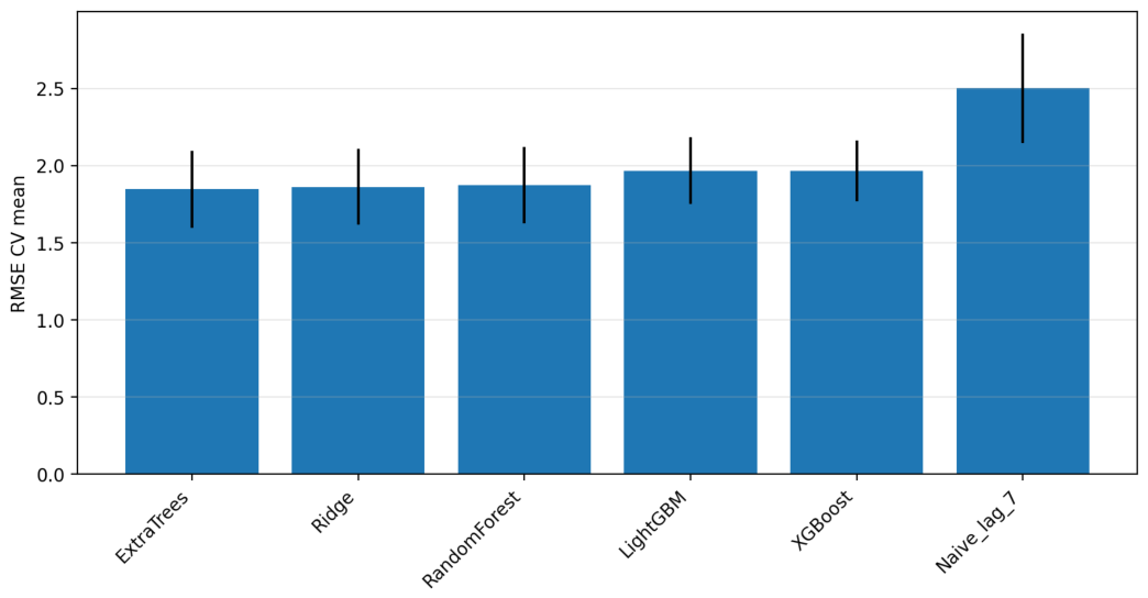
The final test results confirmed that Extra Trees was the best-performing model. It achieved RMSE = 1.6183, MAE = 0.9109, R² = 0.5852, WMAPE = 0.7708, and RMSSE = 0.7226. Compared with the naive weekly benchmark, Extra Trees reduced RMSE from 2.2953 to 1.6183 and MAE from 1.1550 to 0.9109. The R² value indicates that the model explained a meaningful part of the variability in daily product-level sales, although the prediction of real retail demand remained a challenging task. The differences between the best machine learning models were not large. Random Forest, LightGBM, Ridge, and XGBoost also achieved relatively similar predictive performance. Nevertheless, Extra Trees was selected for further interpretability analysis because it obtained the lowest RMSE and the highest R² both in cross-validation and on the final test set.

Step 4. Visual evaluation and error segmentation of the best model

After selecting the Extra Trees model, the relationship between actual and predicted values was analysed. Figure 2 presents the scatter plot of observed and predicted sales values in the final test set.

The plot shows that the model captured low and medium sales levels relatively well. This is important because daily product-level retail sales data contain many observations with zero or low sales. At the same time, larger deviations are visible for observations with high sales values. In particular, some high-demand cases were underestimated by the model. This indicates that sudden demand peaks are more difficult to forecast than regular low and medium sales levels. To further evaluate model performance, an error segmentation analysis was conducted. The purpose of this analysis was to assess whether prediction errors differed across selected groups of observations, including high-sales cases, event days, and SNAP days. The results are presented in Table 4.

The segmentation results confirm that the model performed worse for extreme sales values than for the full test set. In the top 10% sales segment, RMSE increased to 3.7736, while in the top 5% sales segment it increased to 4.9440. This means that high-demand cases were the most difficult to predict. The model also achieved a higher RMSE on event days than on non-event days, which indicates that event-related sales fluctuations increased prediction uncertainty. The results for SNAP and non-SNAP days were more balanced. RMSE was equal to 1.6988 for SNAP days and 1.5718 for non-SNAP days. This suggests that the model maintained relatively stable predictive performance across these two types of days, although prediction errors were slightly higher during SNAP-related periods. Overall, the error analysis indicates that the model is useful for regular product-level sales forecasting, but short-term demand peaks remain more difficult to capture. This has practical implications for retail decision-making, as inventory and promotion planning should account for the higher uncertainty associated with high-sales and event-related observations.

Step 5. Permutation Feature Importance analysis

After selecting the best-performing model, an analysis of feature importance was conducted using the Permutation Feature Importance method. The analysis was performed for the Extra Trees model. The aim of this stage was to determine which variables most strongly influenced predictive quality. Table 5 presents the 10 most important features according to PFI.

Figure 3. Permutation Feature Importance for the Extra Trees model.

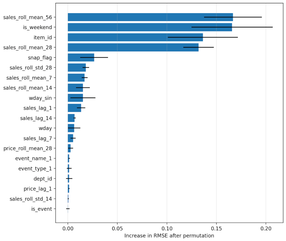
According to PFI, the most important feature was sales_roll_mean_56. The permutation of this variable caused the greatest increase in prediction error, which means that medium-term historical demand was crucial for forecasting future sales. The second most important feature was is_weekend, indicating that weekly sales patterns played a substantial role in the model. The high importance of item_id confirms that product-specific sales behaviour was an essential component of the prediction process. The next important variable was sales_roll_mean_28, which further confirms the relevance of rolling historical demand. Among the top features were also snap_flag, sales_roll_std_28, sales_roll_mean_7, sales_roll_mean_14, wday_sin, and sales_lag_1. These results indicate that the model relied primarily on historical sales levels, weekly calendar structure, product identity, SNAP-related effects, and demand variability.

Step 6. SHAP analysis

For an in-depth interpretation of the Extra Trees model, the SHAP method was applied. SHAP values make it possible to determine the contribution of individual features to model predictions. In this study, SHAP values were aggregated to the level of original variables after preprocessing. The results of the global SHAP analysis are presented in Table 6 and Figure 4.

The SHAP analysis confirmed the results obtained using PFI. The highest mean absolute SHAP value was obtained by sales_roll_mean_56, followed by sales_roll_mean_28, item_id, sales_roll_mean_14, and is_weekend. This means that the model’s predictions were most strongly shaped by medium-term historical demand, product identity, and weekly calendar effects. The presence of sales_roll_std_56 and sales_roll_std_28 among the most important SHAP features indicates that the model also used information about demand variability. Therefore, the model did not rely only on average past sales, but also on the stability or instability of previous demand. The importance of dept_id suggests that the product hierarchy also contributed to the differentiation of sales patterns across departments. The convergence between PFI and SHAP strengthens the interpretation of the model. Both methods indicate that the key determinants of predicted sales were rolling historical demand indicators, product-specific characteristics, weekend effects, SNAP-related information, and demand variability.

Step 7. Necessary Condition Analysis

In the final stage, Necessary Condition Analysis was applied. This method made it possible to move beyond feature-importance ranking and identify variables that may constitute necessary conditions for achieving high sales levels. While PFI and SHAP indicate which features are important for the predictive model, NCA identifies whether a certain minimum level of a given feature is required for a high value of the outcome to occur. The NCA was conducted for the observed value of units_sold. The results are presented in Table 7.

The NCA results indicate that several historical demand and demand-volatility features acted as statistically significant necessary conditions for achieving high sales levels. The strongest statistically significant effects were obtained for sales_roll_std_56 and sales_roll_std_28. This suggests that high sales levels were unlikely to occur when previous demand variability was very low. In practical terms, products with no prior demand movement had limited potential to achieve high sales in the analysed period. Rolling sales averages also appeared as significant necessary conditions. The variables sales_roll_mean_56, sales_roll_mean_28, and sales_roll_mean_14 indicate that a minimum level of historical demand was required for high future sales to be observed. This does not mean that high historical demand was sufficient to guarantee high sales. Rather, it means that high sales were unlikely without at least some preceding demand intensity. The variable price_reduction_vs_roll28 obtained the largest NCA effect size, but its permutation p-value was 0.2600. Therefore, this variable should not be interpreted as a statistically confirmed necessary condition in the analysed sample. It may indicate a potentially relevant price-related pattern, but this pattern was not sufficiently stable in the permutation test. Table 8 presents the NCA bottleneck table for selected variables. The values in the table indicate the minimum level of a given condition required to achieve a selected level of the outcome.

The bottleneck table provides a threshold-based interpretation of the results. For lower outcome levels, the required levels of the analysed conditions were equal to zero. However, for higher outcome levels, especially 90% and 95%, non-zero thresholds appeared for rolling averages and rolling volatility measures. This means that the highest sales levels were observed only when some minimum level of previous demand intensity or previous demand variability was present. The NCA ceiling plots provide a graphical representation of these relationships.

Figure 5. NCA ceiling line for sales_roll_std_56 and observed sales.

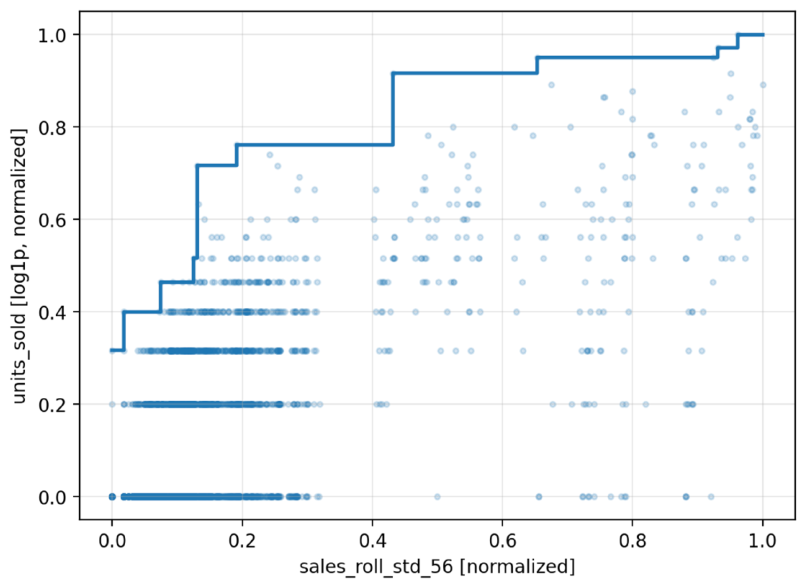
Figure 6. NCA ceiling line for sales_roll_std_28 and observed sales.

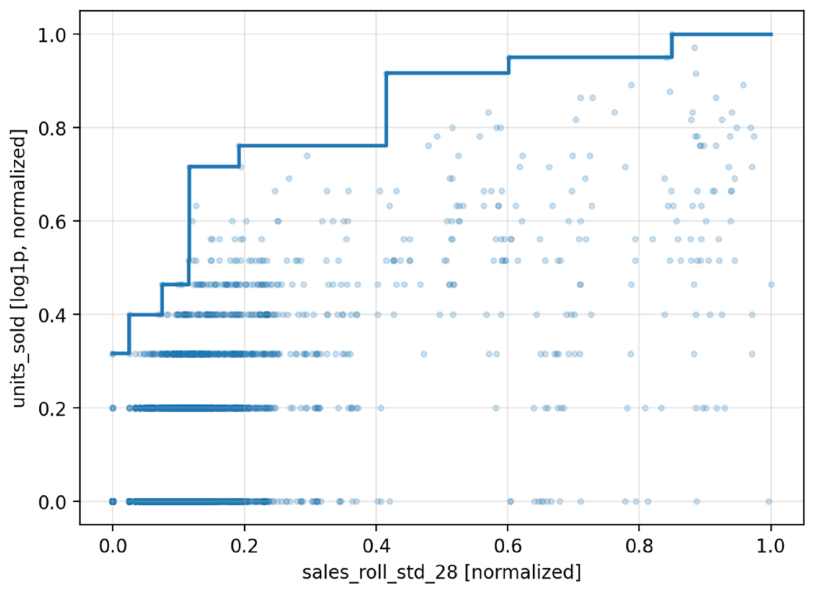
Figure 7. NCA ceiling line for sales_roll_mean_56 and observed sales.

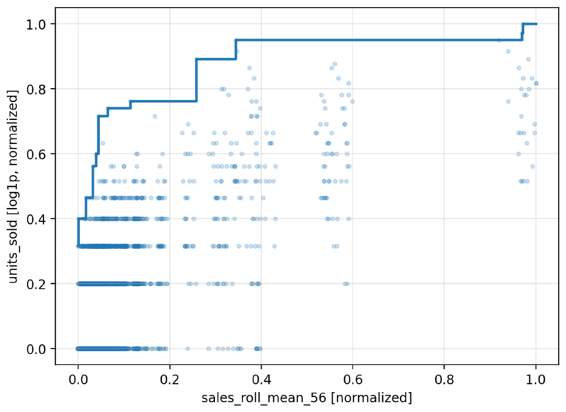
The ceiling plots show the empty-zone logic of Necessary Condition Analysis. The absence of observations in the upper-left part of the plots indicates that high sales levels were not achieved when the analysed condition remained below a certain level. This interpretation complements the SHAP and PFI results. PFI and SHAP show which variables were important for the model, while NCA shows which variables represented bottleneck-like conditions for high sales outcomes. The NCA results are particularly relevant from a decision-making perspective. They suggest that high product sales require not only favourable calendar or product characteristics, but also a minimum level of historical demand or demand variability. Therefore, the proposed ML-XAI-NCA approach makes it possible to interpret sales forecasting not only in terms of prediction accuracy and feature importance, but also in terms of threshold conditions associated with high sales potential.

Discussion

The empirical results demonstrated that the Extra Trees model achieved the best predictive performance among the analysed algorithms. It obtained the lowest RMSE and the highest R² both in rolling-origin cross-validation and in the final test. The model clearly outperformed the naive weekly benchmark, which confirms the usefulness of machine learning models in product-level sales forecasting. The PFI and SHAP analyses showed that the most important predictors of sales were historical rolling averages, product identity, weekend effects, SNAP-related information, and rolling demand volatility. These results indicate that the model relied primarily on previous demand dynamics and product-specific sales patterns. The NCA extended the interpretation of the results by identifying necessary conditions for achieving high sales levels. The analysis showed that selected rolling averages and rolling volatility measures represented statistically significant bottleneck-like conditions. This means that the highest sales levels were unlikely without a minimum level of previous demand intensity or previous demand variability. The integration of model benchmarking, PFI, SHAP, and NCA provided a comprehensive view of the forecasting problem. Model benchmarking identified the most accurate algorithm, XAI methods explained the main determinants of model predictions, and NCA translated selected predictors into threshold-based conditions associated with high sales outcomes.

Conclusion

The aim of this article was to develop and evaluate a predictive framework for product sales forecasting using selected machine learning regression algorithms, model interpretability methods, and Necessary Condition Analysis. The study was based on real product-level retail sales data from the Walmart M5 dataset and incorporated calendar, product hierarchy, event-related, price-related, and historical demand features. The empirical procedure combined model benchmarking, rolling-origin validation, final test-set evaluation, error segmentation, Permutation Feature Importance, SHAP analysis, and Necessary Condition Analysis.

The conducted experiment demonstrated that, among the analysed algorithms, the best results were obtained by the Extra Trees model. This model achieved the lowest prediction error and the highest coefficient of determination both in rolling-origin cross-validation and on the final 28-day test set. On the final test set, Extra Trees achieved RMSE = 1.6183, MAE = 0.9109, R² = 0.5852, WMAPE = 0.7708, and RMSSE = 0.7226. The model also clearly outperformed the naive weekly benchmark based on sales from seven days earlier. This confirms the usefulness of machine learning models in product-level sales forecasting, especially when the input data include historical demand patterns, product-specific characteristics, calendar effects, and price-related information.

The theoretical contribution of this article consists in proposing an integrated ML-XAI-NCA framework for product sales forecasting. The results show that the evaluation of predictive quality alone is not sufficient for a full understanding of the model’s operation. Therefore, model benchmarking was complemented with two types of explanation. First, PFI and SHAP were used to identify the most important predictors of sales. Second, NCA was used to determine whether selected predictors constituted necessary conditions for achieving high sales levels. This approach extends standard explainable forecasting procedures by moving beyond feature-importance rankings toward the identification of threshold-like bottlenecks associated with high sales outcomes.

The PFI and SHAP analyses indicated that the key determinants of predicted sales were primarily historical rolling sales averages, product identity, weekend effects, SNAP-related information, and rolling demand volatility. The high importance of variables such as sales_roll_mean_56, sales_roll_mean_28, sales_roll_mean_14, and item_id shows that the model relied strongly on medium-term historical demand and product-specific sales behaviour. The importance of is_weekend, wday_sin, and snap_flag additionally confirms the role of weekly calendar structure and selected event-related conditions in shaping daily retail sales.

The Necessary Condition Analysis provided an additional layer of interpretation. The results showed that selected rolling averages and rolling standard deviations of past sales acted as statistically significant necessary conditions for achieving high sales levels. In particular, sales_roll_std_56, sales_roll_std_28, sales_roll_mean_56, sales_roll_mean_28, and sales_roll_mean_14 were identified as bottleneck-like variables. This means that high sales levels were unlikely without at least a minimum level of previous demand intensity or previous demand variability. At the same time, these conditions should not be interpreted as sufficient causes of high sales. Rather, they indicate the minimum historical demand-related conditions under which high sales become feasible.

From a practical perspective, the obtained results may support managerial decisions in retail and e-commerce-related sales management. The proposed framework can be used not only to forecast future product sales but also to identify demand-related signals associated with high sales potential. Information derived from PFI and SHAP may help managers understand which features are most relevant for model predictions, whereas NCA bottleneck tables may support threshold-oriented decision-making. For example, products with insufficient historical demand intensity or very low demand variability may require more cautious inventory planning, while products satisfying the identified necessary conditions may deserve closer attention in replenishment, promotion planning, or price monitoring processes. The error segmentation analysis also showed that extreme sales values and event-related observations are more difficult to forecast, which suggests that such cases should be treated as higher-risk situations in operational planning.

The study has several limitations. First, the empirical analysis was conducted on a selected sample of product-store series from the Walmart M5 dataset, which made it possible to ensure computational feasibility but may limit the generalizability of the results to the full hierarchy of products and stores. Second, the analysis focused on point forecasting of daily unit sales, while probabilistic forecasts, prediction intervals, and multi-horizon forecasting were not examined. Third, the dataset did not include some variables that may be important in real business practice, such as detailed inventory availability, online traffic, advertising expenditure, product ratings, returns, and local promotion intensity. Fourth, although the NCA results provide useful information on necessary conditions, they should be interpreted as threshold-oriented empirical patterns rather than as proof of causal sufficiency.

Future research should extend the analysis to a broader set of product-store series and different levels of the sales hierarchy, including product, department, category, store, and state-level aggregation. It would also be valuable to compare the proposed ML-XAI-NCA framework with probabilistic forecasting models, deep learning architectures, and hierarchical forecasting methods. A further direction for future work may involve the integration of additional operational variables, such as inventory levels, stockout indicators, marketing activity, and promotion intensity. Finally, future studies could examine the stability of SHAP, PFI, and NCA results over time and assess whether the identified necessary conditions can be used in real-world decision-support systems for inventory replenishment, promotion planning, and dynamic pricing.

References

Benidis, K., Rangapuram, S. S., Flunkert, V., Wang, Y., Maddix, D., Turkmen, C., Gasthaus, J., Bohlke-Schneider, M., Salinas, D., Stella, L., & others. (2022). Deep learning for time series forecasting: Tutorial and literature survey. ACM Computing Surveys, 55(6), 1–36.
Breiman, L. (2001). Random forests. Machine Learning, 45(1), 5–32.
Chen, S., Ke, S., Han, S., Gupta, S., & Sivarajah, U. (2024). Which product description phrases affect sales forecasting? An explainable AI framework by integrating WaveNet neural network models with multiple regression. Decision Support Systems, 176, 114065.
Chen, T., & Guestrin, C. (2016). Xgboost: A scalable tree boosting system. Proceedings of the 22nd Acm Sigkdd International Conference on Knowledge Discovery and Data Mining, 785–794.
Dul, J. (2016). Necessary condition analysis (NCA) logic and methodology of “necessary but not sufficient” causality. Organizational Research Methods, 19(1), 10–52.
Dul, J. (2024). A different causal perspective with necessary condition analysis. Journal of Business Research, 177, 114618.
Dul, J., der Laan, E., & Kuik, R. (2020). A statistical significance test for necessary condition analysis. Organizational Research Methods, 23(2), 385–395.
Dul, J., Hauff, S., & Bouncken, R. B. (2023). Necessary condition analysis (NCA): review of research topics and guidelines for good practice: J. Dul et al. Review of Managerial Science, 17(2), 683–714.
Ferreira, K. J., Lee, B. H. A., & Simchi-Levi, D. (2016). Analytics for an online retailer: Demand forecasting and price optimization. Manufacturing & Service Operations Management, 18(1), 69–88.
Fildes, R., Ma, S., & Kolassa, S. (2022). Retail forecasting: Research and practice. International Journal of Forecasting, 38(4), 1283–1318.
Fisher, A., Rudin, C., & Dominici, F. (2019). All models are wrong, but many are useful: Learning a variable’s importance by studying an entire class of prediction models simultaneously. Journal of Machine Learning Research, 20(177), 1–81.
Hoerl, A. E., & Kennard, R. W. (1970). Ridge regression: Biased estimation for nonorthogonal problems. Technometrics, 12(1), 55–67.
Huber, J., & Stuckenschmidt, H. (2020). Daily retail demand forecasting using machine learning with emphasis on calendric special days. International Journal of Forecasting, 36(4), 1420–1438.
Hyndman, R. J., & Athanasopoulos, G. (2018). Forecasting: principles and practice. OTexts.
Hyndman, R. J., & Koehler, A. B. (2006). Another look at measures of forecast accuracy. International Journal of Forecasting, 22(4), 679–688.
John Lu, Z. Q. (2010). The elements of statistical learning: data mining, inference, and prediction. Oxford University Press.
Ke, G., Meng, Q., Finley, T., Wang, T., Chen, W., Ma, W., Ye, Q., & Liu, T.-Y. (2017). Lightgbm: A highly efficient gradient boosting decision tree. Advances in Neural Information Processing Systems, 30.
Lim, B., Ark, S. Ö., Loeff, N., & Pfister, T. (2021). Temporal fusion transformers for interpretable multi-horizon time series forecasting. International Journal of Forecasting, 37(4), 1748–1764.
Lundberg, S. M., & Lee, S.-I. (2017). A unified approach to interpreting model predictions. Advances in Neural Information Processing Systems, 30.
Ma, S., & Fildes, R. (2021). Retail sales forecasting with meta-learning. European Journal of Operational Research, 288(1), 111–128.
Makridakis, S., Spiliotis, E., & Assimakopoulos, V. (2020). The M4 Competition: 100,000 time series and 61 forecasting methods. International Journal of Forecasting, 36(1), 54–74.
Makridakis, S., Spiliotis, E., & Assimakopoulos, V. (2022). The M5 competition: Background, organization, and implementation. International Journal of Forecasting, 38(4), 1325–1336.
Nowak, M., & Zajkowski, R. (2025). An Integrated Structural Equation Modelling and Machine Learning Framework for Measurement Scale Evaluation—Application to Voluntary Turnover Intentions. AppliedMath, 5(3), 105.
Oreshkin, B. N., Carpov, D., Chapados, N., & Bengio, Y. (2019). N-BEATS: Neural basis expansion analysis for interpretable time series forecasting. ArXiv Preprint ArXiv:1905.10437.
Ribeiro, M. T., Singh, S., & Guestrin, C. (2016). “ Why should i trust you?” Explaining the predictions of any classifier. Proceedings of the 22nd ACM SIGKDD International Conference on Knowledge Discovery and Data Mining, 1135–1144.
Salinas, D., Flunkert, V., Gasthaus, J., & Januschowski, T. (2020). DeepAR: Probabilistic forecasting with autoregressive recurrent networks. International Journal of Forecasting, 36(3), 1181–1191.
Shapley, L. S., & others. (1953). A value for n-person games.
Spiliotis, E., Makridakis, S., Semenoglou, A.-A., & Assimakopoulos, V. (2022). Comparison of statistical and machine learning methods for daily SKU demand forecasting. Operational Research, 22(3), 3037–3061.
Theodorou, E., Spiliotis, E., & Assimakopoulos, V. (2025). Forecast accuracy and inventory performance: Insights on their relationship from the M5 competition data. European Journal of Operational Research, 322(2), 414–426.
Theodorou, E., Wang, S., Kang, Y., Spiliotis, E., Makridakis, S., & Assimakopoulos, V. (2022). Exploring the representativeness of the M5 competition data. International Journal of Forecasting, 38(4), 1500–1506.
Wang, L., & Zhang, X. (2024). Livestream sales prediction based on an interpretable deep-learning model. Scientific Reports, 14(1), 20594.
Wellens, A. P., Boute, R. N., & Udenio, M. (2024). Simplifying tree-based methods for retail sales forecasting with explanatory variables. European Journal of Operational Research, 314(2), 523–539.

Figure 2. Relationship between actual and predicted sales values for the Extra Trees model.

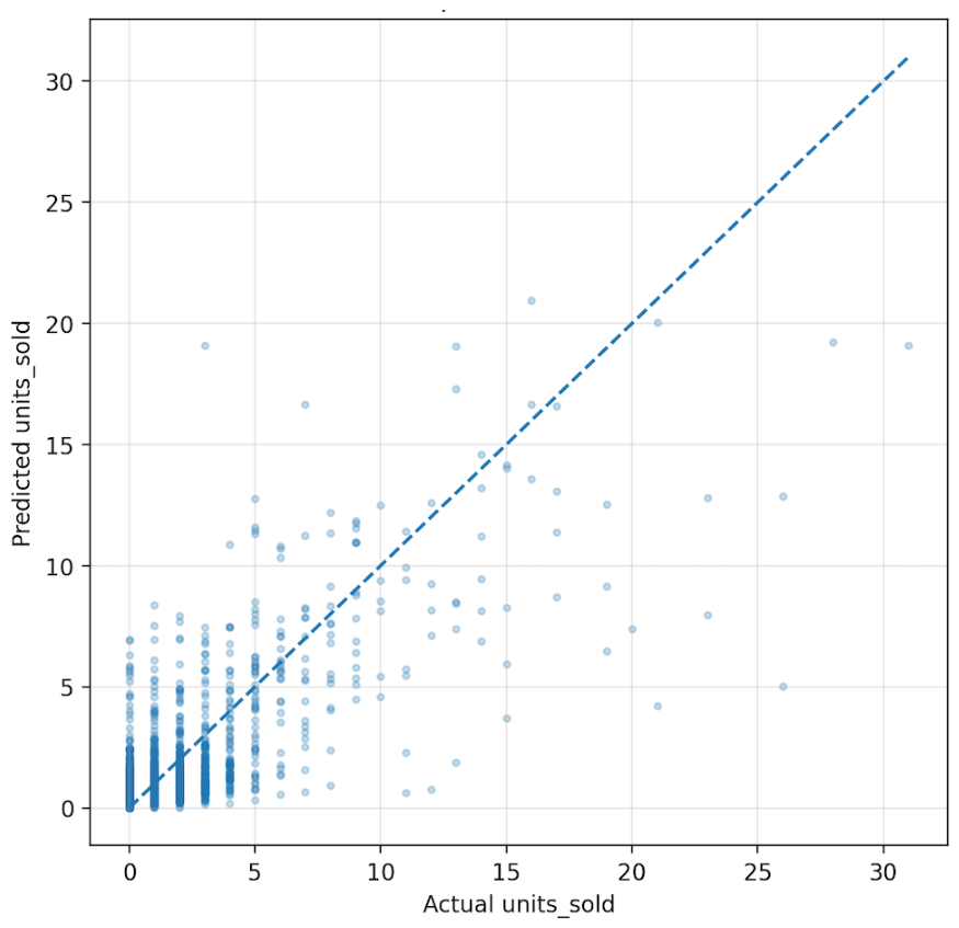
Figure 4. Global feature importance according to SHAP values for the Extra Trees model.

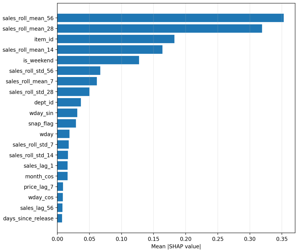
Table 1. The dataset for the product sales prediction model.

Variable group	Variables	Description
Target variable	units_sold	The number of product units sold on a given day; this was the value predicted by the models.
Product and hierarchy features	item_id, dept_id, cat_id, store_id, state_id	Variables identifying the product, department, category, store, and state. They allow the model to capture differences in sales patterns across products and locations.
Calendar features	wday, month, year, is_weekend, wday_sin, wday_cos, month_sin, month_cos	Variables representing weekly and monthly sales patterns, seasonality, and cyclical calendar effects.
Event-related features	event_name_1, event_type_1, is_event	Variables indicating the occurrence and type of special events that may influence demand.
SNAP-related features	snap_flag	A binary indicator identifying SNAP-related days in a given state.
Price-related features	sell_price, price_lag_1, price_lag_7, price_roll_mean_28, price_reduction_vs_roll28	Variables describing the current product price and changes in price relative to previous periods.
Lagged sales features	sales_lag_1, sales_lag_7, sales_lag_14, sales_lag_28, sales_lag_56	Historical sales values from previous days, reflecting short-term and medium-term demand memory.
Rolling sales averages	sales_roll_mean_7, sales_roll_mean_14, sales_roll_mean_28, sales_roll_mean_56	Rolling averages of past sales, representing local demand trends over different time windows.
Rolling sales volatility	sales_roll_std_7, sales_roll_std_14, sales_roll_std_28, sales_roll_std_56	Rolling standard deviations of past sales, representing the variability of demand over different time windows.
Additional time-related features	days_since_release	A variable describing the number of days since the product appeared in the sales data.

Table 2. Results of rolling-origin cross-validation.

Model	RMSE mean	RMSE std	MAE mean	R² mean	WMAPE mean	RMSSE mean
ExtraTrees	1.8461	0.2485	0.9209	0.5145	0.7892	0.7072
Ridge	1.8620	0.2447	0.9098	0.5060	0.7797	0.7309
RandomForest	1.8742	0.2474	0.9643	0.4996	0.8268	0.7265
LightGBM	1.9661	0.2168	0.9592	0.4498	0.8223	0.7168
XGBoost	1.9668	0.1976	0.9583	0.4489	0.8216	0.7143
Naive_lag_7	2.5006	0.3542	1.1344	0.1113	0.9712	0.9657

Table 3. Final test results.

Model	RMSE	MAE	R²	WMAPE	RMSSE
ExtraTrees	1.6183	0.9109	0.5852	0.7708	0.7226
RandomForest	1.6581	0.9494	0.5646	0.8033	0.7306
LightGBM	1.6770	0.9430	0.5546	0.7979	0.7276
Ridge	1.6885	0.9167	0.5484	0.7756	0.7376
XGBoost	1.6898	0.9378	0.5478	0.7935	0.7267
Naive_lag_7	2.2953	1.1550	0.1656	0.9773	0.9808

Table 4. Error analysis by selected test-set segments.

Segment	n	RMSE	MAE	R²	WMAPE
all_test	3052	1.6183	0.9109	0.5852	0.7708
top_10pct_sales	393	3.7736	2.6892	0.2799	0.4522
top_5pct_sales	179	4.9440	3.5612	0.0398	0.3935
event_days	436	1.8451	0.9960	0.4763	0.7411
non_event_days	2616	1.5773	0.8968	0.6037	0.7765
snap_days	1090	1.6988	0.9370	0.6241	0.7249
non_snap_days	1962	1.5718	0.8964	0.5546	0.8002

Table 5. The 10 most important features in the PFI analysis.

Feature	Importance mean	Importance std
sales_roll_mean_56	0.1667	0.0291
is_weekend	0.1658	0.0410
item_id	0.1363	0.0353
sales_roll_mean_28	0.1319	0.0154
snap_flag	0.0265	0.0140
sales_roll_std_28	0.0181	0.0034
sales_roll_mean_7	0.0169	0.0030
sales_roll_mean_14	0.0152	0.0069
wday_sin	0.0152	0.0127
sales_lag_1	0.0134	0.0042

Table 6. Top 10 features according to the SHAP method.

Feature	Mean absolute SHAP value
sales_roll_mean_56	0.3529
sales_roll_mean_28	0.3191
item_id	0.1825
sales_roll_mean_14	0.1638
is_weekend	0.1273
sales_roll_std_56	0.0668
sales_roll_mean_7	0.0617
sales_roll_std_28	0.0501
dept_id	0.0368
wday_sin	0.0310

Table 7. Necessary Condition Analysis results for observed sales.

Feature	NCA effect size d	Permutation p-value
price_reduction_vs_roll28	0.5030	0.2600
sales_roll_std_56	0.1821	0.0100
sales_roll_std_28	0.1714	0.0100
sales_roll_mean_56	0.1162	0.0100
sales_roll_std_14	0.1153	0.0100
sales_roll_mean_28	0.1133	0.0100
sales_roll_mean_14	0.0862	0.0100
sales_roll_std_7	0.0843	0.0100
sales_roll_mean_7	0.0755	0.0100
sales_lag_28	0.0436	0.0100

Table 8. NCA bottleneck table for selected necessary conditions.

Feature	90% outcome level	95% outcome level
sales_roll_mean_14	0.0714	0.0714
sales_roll_mean_28	0.0357	0.3571
sales_roll_mean_56	0.0179	0.4643
sales_roll_std_14	0.2673	0.2673
sales_roll_std_28	0.1890	0.8751
sales_roll_std_56	0.1336	0.9200
sales_roll_std_7	0.0000	0.0000

Disclaimer/Publisher’s Note: The statements, opinions and data contained in all publications are solely those of the individual author(s) and contributor(s) and not of MDPI and/or the editor(s). MDPI and/or the editor(s) disclaim responsibility for any injury to people or property resulting from any ideas, methods, instructions or products referred to in the content.

© 2026 by the authors. Licensee MDPI, Basel, Switzerland. This article is an open access article distributed under the terms and conditions of the Creative Commons Attribution (CC BY) license (http://creativecommons.org/licenses/by/4.0/).

Copyright: This open access article is published under a Creative Commons CC BY 4.0 license, which permit the free download, distribution, and reuse, provided that the author and preprint are cited in any reuse.

Explainable Machine Learning and Necessary Condition Analysis for Product Sales Forecasting in Retail

Abstract

Keywords:

Subject:

Introduction

Methods

Results

Discussion

Conclusion

References

MDPI Initiatives

Important Links

Subscribe