
Submitted:
07 July 2026
Posted:
08 July 2026
You are already at the latest version
Abstract
The evaluation of Gridded Precipitation Products (GPPs) must account for the zero-inflated nature of precipitation data and the differences in spatial support between rain gauges and satellite grids. This study assesses the timing, precipitation event detection, and volume of ERA5, IMERG, CHIRPS, and TAMSAT against the Trans-African Hydro-Meteorological Observatory (TAHMO) network. We employ variance-stabilising transformations, detect rainfall events, and cluster diurnal precipitation cycles into different regimes. Our clustering results reveal spatial variability in performance, with GPP and TAHMO derived diurnal regimes differing at 57.3% of the stations. Analysis of the diurnal precipitation reveals that ERA5 satisfies its daily water budget through persistent drizzle. At the daily scale, IMERG exhibits superior event detection, timing, and volume accuracy. On the other hand, CHIRPS and TAMSAT show a wet bias. We conclude that GPP selection should consider the use-case, and future meteorological and AI-driven applications should incorporate verification metrics that account for timing, event detection and volume accuracy.
Keywords:
Gridded Precipitation Products
; variance-stabilisation
; phase alignment
; water budget
; event detection
; drizzle bias
; diurnal cycle
1. Introduction
The accurate estimation of precipitation is a fundamental prerequisite for hydrological modelling, agricultural forecasting, and flood risk management [1,2]. In East Africa, where the spatiotemporal variability of rainfall is heavily influenced by the interplay of the Intertropical Convergence Zone [3], complex topography, and local convective instability, the scarcity of ground-based gauge networks presents a bottleneck [4]. Consequently, hydrologists increasingly rely on GPPs, including satellite-based estimates such as IMERG [5] and CHIRPS [6], and reanalysis products like ERA5 [7], to serve as input for hydrological models [8].
However, the utility of these GPPs is often limited by systematic discrepancies when compared to ground observations. Traditional validation studies employ point-to-grid comparisons using error metrics such as Root Mean Square Error (RMSE), Mean Bias Error (MBE), and the Kling-Gupta Efficiency (KGE) on raw precipitation data [9,10]. While traditional metrics provide a necessary assessment of volume accuracy, they are often insufficient for diagnosing the underlying mechanisms of a model’s failure. For instance, a dataset may achieve a satisfactory daily volume by simulating persistent, low-intensity drizzle rather than the actual observed short-duration, high-intensity rain events [11,12,13]. On the other hand, a high-resolution satellite might capture a physical rainfall event correctly, but standard metrics will score it as a total failure simply because the rain event was recorded slightly in the wrong place or at the wrong time [14].
This rigidity gives rise to the “double penalty” problem—where a GPP dataset is penalised once for missing the exact timing or location of a rain event, and again for predicting the wrong intensity, hiding the dataset’s true skill [15]. Research in forecast validation has suggested moving beyond rigid point-to-point matching toward fuzzy, neighbourhood-based evaluations [16] and pattern-based evaluations [17]. By evaluating predictions within a spatial or temporal window of tolerance, these neighbourhood approaches disentangle timing accuracy from volume accuracy. Distinguishing whether a dataset fails due to a temporal phase misalignment or simply because it suffers from volumetric attenuation is critical for developing effective bias-correction strategies [18].
In this study, we perform an analysis of four widely used precipitation products: ERA5, IMERG, TAMSAT, and CHIRPS, against the Trans-African Hydro-Meteorological Observatory (TAHMO) network, which at the time of writing, has 332 stations across the East African region [19]. While recent studies have successfully leveraged the TAHMO network to expose volumetric biases in satellite products [20], these evaluations have predominantly relied on standard, raw-space linear metrics aggregated at daily or monthly scales. Consequently, the sub-daily physical mechanisms driving these errors often remain obscured. To address this, our methodology is two-fold. First, we address the extreme skewness of daily precipitation distributions by applying variance-stabilising transformations, enabling the assessment of signal consistency within a variance-stabilised “transformed space” of the data [21,22]. Second, we evaluate the timing consistency of these signals. By partitioning the data into 30-day overlapping windows, we apply a time-shifting technique combined with a Gaussian temporal filter. This allows us to identify the best possible timing alignment for the rainfall events within each specific temporal window.
This approach allows us to answer two critical questions regarding the observed differences between datasets: First, are these deviations driven by a fundamental lack of physical signal correlation, or by a systematic temporal misalignment? Second, to what extent do the GPPs and point-scale observations differ regarding the diurnal precipitation cycle in East Africa? By extending our analysis to the diurnal scale, we aim to identify the structural mechanisms that influence the performance characteristics of GPPs. The findings presented here offer a perspective on GPP selection, suggesting that the selection of the “appropriate” GPP depends on the use-case, considering and prioritising either the accurate timing and frequency of precipitation events [23] or the conservation of total rainfall volume required for processes such as downscaling [24].
2. Materials and Methods
2.1. Study Area and Data Acquisition
The study domain encompasses the East African region, covering Kenya, Uganda, Tanzania, Rwanda, and Burundi (Figure 1) between 2018 to 2024. This region is positioned approximately between latitudes 5°N and 12°S, and longitudes 29°E and 42°E; it is characterised by highly complex topography that heavily influences local weather patterns. Elevations range from sea level along the eastern Indian Ocean coastline to regions exceeding 5,000 meters above sea level (such as Mount Kenya and Mount Kilimanjaro). Furthermore, features like the Great Rift Valley and Lake Victoria create distinct, localised microclimates [25,26]. This topographical variation drives the complex, localised rainfall patterns—and the highly varied diurnal precipitation cycles—that make precipitation evaluation in this region particularly challenging.
2.1.1. Station Network (TAHMO)
2.1.2. Gridded Precipitation Products (GPPs)
We evaluated four widely used GPPs representing different estimation methodologies: Reanalysis (ERA5), Satellite-Infrared (TAMSAT), Satellite-Microwave merged (IMERG), and Blended Satellite-Gauge (CHIRPS). Table 1 summarises the product characteristics.
2.2. Data Pre-Processing and Quality Control
2.2.1. Station Selection and Temporal Alignment
To ensure robust statistical comparisons, a filtering protocol was applied to the TAHMO network:
- Daily Completeness: For daily aggregation, a station was considered valid only if at least 21 out of 24 hourly records were present.
- Series Continuity and hourly completeness: Stations missing more than 30% of hourly data over the 7-year study period were excluded.
- Temporal Intersection: To eliminate sampling bias, we obtained the intersection of valid timestamps across all datasets and only retained timestamps where the TAHMO station and the GPPs had valid data.
This filtering process yielded 117 stations meeting the daily completeness criteria and 122 stations meeting the series continuity requirements. To maintain a consistent spatial footprint across all evaluations, the final observation network was restricted to the subset of 117 stations. Prior to evaluation, the datasets were aggregated into daily totals for the rolling windows analysis, and the sub-daily datasets (IMERG, ERA5 and TAHMO) into hourly intervals to evaluate the diurnal cycle.
2.3. Methodology
The sections below discuss the methodological framework that we applied in our analysis.
2.3.1. Variance Stabilisation and Transformed Space
Daily precipitation data exhibits extreme positive skewness and zero-inflation. To address this, we transformed all data into a variance-stabilised “transformed space” [21] using two methods:
-
Box-Cox Transformation: Defined by Equation (1) below:where:
- –
- represents the transformed precipitation value,
- –
- x is the raw precipitation intensity
- –
- is an optimised offset derived from the data to accommodate zero-inflation
- –
- is the shape parameter governing the severity of the transformation [28].
These parameters are tuned independently; this effectively projects each GPP–TAHMO pair into a distinct, independent transformed space that accommodates the unique distributional characteristics (e.g., specific zero-inflation or tail behavior) of that product. -
Inverse Hyperbolic Sine (ArcSinh) Transformation: We applied the Inverse Hyperbolic Sine transformation as an alternative to the Box-Cox transformation to handle extreme values [22], as defined by Equation (2) below:where:
- –
- y represents the transformed precipitation value
- –
- x is the raw precipitation intensity.
To maintain mathematical consistency for pairwise comparison, the optimal transformation parameters ( and offset ) derived from a specific GPP were subsequently applied to the corresponding TAHMO station series. If the ground observations and the gridded predictions were transformed independently using their own optimal parameters, the two signals would be projected into entirely different dimensional spaces. This scale mismatch would render relative amplitude comparisons—such as the Kling-Gupta Bias and Variability ratios mathematically invalid.
Instead, our methodology projects TAHMO data into the specific variance-stabilised “transformed space” of each individual GPP. For example, in the Box-Cox space optimised for ERA5, physical rainfall thresholds (e.g., ) are translated into an exact variance-stabilised equivalent () using ERA5’s specific and parameters. Both the TAHMO and ERA5 signals are then evaluated against this shared threshold.
This approach ensures that the evaluation metrics consider true phase dynamics while preserving the distinction between wet and dry states. Because GPPs parameterise dry states distinctly—such as ERA5 exhibiting a persistent trace drizzle bias [11], mapping TAHMO data into the GPP’s native transformed space forces the statistical evaluation to test whether the GPP correctly times its own version of a wet event against the physical occurrence of rain.
2.3.2. Spatial Interpolation, Variance Stabilisation, and Kernel Optimisation
To extract gridded data at specific station coordinates, we compared Nearest Neighbour interpolation against Bilinear Interpolation as a preliminary step.
This preliminary evaluation was conducted on the raw, unsmoothed daily time series () prior to any variance stabilisation, ensuring that temporal smoothing did not blur the interpolation artifacts. For each station, we computed the Pearson correlation coefficient (r) between the ground gauge and the GPP signal. We then calculated the arithmetic mean of the station-level correlation differences () across the observational network.
We also compared the Pearson correlation values of each GPP-TAHMO pair at various kernel widths for the Gaussian temporal smoothing (ranging from 0 to 21 days) to determine the optimal kernel width.
We then evaluated the correlation of the entire historical time series without applying temporal rolling windows. The Pearson correlation coefficient (r) was calculated independently at every valid TAHMO station to capture localised spatial dynamics. To quantify the overall efficacy of a transformation method (e.g., Box-Cox, ArcSinh), we aggregated these station-level correlations to construct a network-wide performance distribution. The most appropriate transformation for each GPP was then determined by evaluating the central tendency (median and arithmetic mean) and the interquartile spread of these station-level correlations. This ensured that the selected mathematical transformation structurally preserved or enhanced the baseline temporal signal across the majority of the spatial domain prior to conducting the localised phase-shift analysis.
2.3.3. Gaussian Temporal Smoothing
To analyze the consistency of large-scale weather patterns and dampen the effect of minor timing mismatches, we applied a 1D Gaussian smoothing kernel to all time series as shown by Equation (3) below:
where:
- is the temporally smoothed precipitation value at the target day t,
- is the raw, unshifted precipitation value at day ,
- is the standard deviation of the Gaussian kernel, governing the temporal spread of the smoothing filter,
- represents the temporal indices within the localised rolling window surrounding t.
We used this to compare the Pearson correlation values of each GPP-TAHMO pair at various kernel widths for the Gaussian temporal smoothing (ranging from 0 to 21 days) to determine the optimal kernel width.
2.3.4. Rolling Window Cross-Correlation Analysis
To diagnose non-stationary temporal misalignments, we performed a rolling window analysis on the transformed data. The time series was partitioned into 30-day windows (total windows). Within each window, we:
- Applied a temporal shift to the GPP signal ranging from days.
- Calculated the similarity between the shifted GPP signal and the unshifted TAHMO signal.
- Identified the optimal shift that maximised the performance metric.
Windows exhibiting zero variance (for example all zeros) were flagged and excluded from the correlation analysis to prevent numerical instability.
2.4. Performance Metrics and Scoring
To evaluate the spatiotemporal coherence of the GPPs, we employed a scoring framework that prioritises phase dynamics and event detection capability over simple amplitude matching. This approach mitigates the “double penalty” problem inherent in point-to-grid comparisons, particularly within the transformed space.
2.4.1. Window-Level Optimisation and Event Detection
The fundamental unit of analysis was the 30-day time window (). For each window k, station s, and dataset d, we evaluated the optimal temporal alignment between each GPP–TAHMO pair by maximising the cross-correlation function over a temporal lag window days.
To evaluate the underlying phase of the atmospheric signal, the transformed GPP time series was first shifted by lag , after which both the baseline transformed TAHMO signal and the shifted GPP signal were processed concurrently through a Gaussian smoothing filter. The optimal Pearson Correlation () is calculated on these smoothed continuous signals using Equation (4) below:
where:
- is the optimal correlation achieved at station s during window k
- is the applied temporal lag, is the set of temporal indices within window k
- represents the transformed and smoothed TAHMO signal at time t
- represents the transformed and smoothed GPP signal at time t offset by the temporal lag
- represents the arithmetic mean of over the window
- represents the arithmetic mean of over the window.
Event Detection
Evaluating rain event detection on smoothed data artificially flattens sharp, high-intensity convective peaks, causing them to fall below detection thresholds and unfairly penalise datasets. To address this, we evaluated event detection using the Critical Success Index (CSI) [29] via a two-tiered approach: temporal point-to-point CSI and temporal neighbourhood (fuzzy) CSI.
A physical rainfall threshold of was translated into the equivalent variance-stabilised threshold () using the respective Box-Cox or ArcSinh parameters.
First, the point-to-point () was computed on the unsmoothed transformed data to evaluate exact temporal precision using Equation (5):
where:
- are hits
- are false alarms
- are misses,
which was calculated by evaluating the unshifted raw signals directly against .
Second, we computed a fuzzy Critical Success Index () by transitioning from strict point-to-point matching to a temporal neighbourhood approach. While this metric retains the exact formulation of the point-to-point CSI, the data processing pipeline proceeded in three sequential steps:
- 1.
- Binarisation: Transformed precipitation signals were converted to binary events, where daily totals exceeding the physical threshold () equalled 1.0, and values below equalled 0.0.
- 2.
- Gaussian Smoothing: A Gaussian filter ( days) was applied to the binary vectors. This transformed isolated, discrete rain days into continuous probability curves bounded within .
- 3.
- Threshold Evaluation: These smoothed curves were evaluated against a strict probability threshold to derive the resulting hits, misses, and false alarms.
For an isolated precipitation event recorded by TAHMO at day , the continuous probability profile at a temporal shift of days is defined by the Gaussian kernel function in Equation (6):
Using a kernel width of days, setting the threshold at creates an operational window to evaluate how closely the GPPs align with TAHMO:
- Exact Alignment (0-day shift): A direct daily match () yields a peak probability of , successfully registering as a Hit.
- Acceptable Shift (-day shift): A 1-day shift () yields . Because this stays above the boundary, the dataset is rewarded for maintaining close temporal consistency.
- Unacceptable Shift (-day shift): A 2-day shift () yields . Falling below the threshold, this divergence is penalised as a Miss.
By positioning the threshold between the 1-day and 2-day discrete intervals—which equates to a continuous temporal radius of days—the framework establishes a cutoff for daily observations. This selection is motivated by the operational requirements of the East African domain: it forgives minor 1-day physical timing shifts caused by convective phase lags, while rejecting displacements of 2 days or more that would be unsuitable for agricultural planning or early flood warnings.
Physical Scaling and Variability
We computed the Kling-Gupta Efficiency (KGE) components for each window on the smoothed signals to diagnose intensity and variability errors using ratios as shown in Equation (7):
where:
- is the volumetric bias ratio for the specific temporal window k
- is the variability ratio for the specific temporal window k
- and represent the arithmetic means of the GPP and TAHMO precipitation signals, respectively, calculated over the duration of window k in the transformed space
- and denote the standard deviations of the GPP and TAHMO precipitation signals, respectively, within window k.
Because these statistics are computed on variance-stabilised data, their physical interpretation differs from standard metrics. quantifies the shift in the Typical Intensity State (e.g., indicating whether a GPP’s baseline behavior simulates physical dry days or parameterised drizzle), while measures the signal’s ability to reproduce the full span of observed weather fluctuations.
2.4.2. Station-Level Scoring
To aggregate performance across all temporal windows for a single station, we defined a bounded Composite Score (). Aggregating the Kling-Gupta Bias () and Variability () ratios presents two distinct mathematical challenges: ratio asymmetry and state mismatches.
First, simple arithmetic averaging of ratios introduces asymmetry errors. For example, a GPP that overestimates by double () in one window and subsequently underestimates by half () in the next yields an arithmetic mean of 1.25. This falsely implies a systematic 25% overestimation, despite the GPP being balanced overall.
Second, within the variance-stabilised transformed space, datasets may disagree on the weather state. For instance, a GPP might register a precipitation event (yielding a positive transformed value), while the gauge registers physical dry noise (yielding a negative transformed value). This “state mismatch” results in a negative ratio, which is physically uninterpretable for volumetric scaling and mathematically undefined for logarithmic transformation. Furthermore, the CSI scores already capture rain event detection, effectively penalising these state mismatches.
To address these issues, we first filtered the evaluation to isolate valid windows (V) where both datasets agreed on the overall distributional state (). The true aggregate physical bias was then calculated using the geometric mean of these valid ratios, preventing arithmetic asymmetry, as defined in Equation (8):
Because the final Composite Score requires evaluation metrics to operate on a normalised scale, these unbounded physical ratios ( and ) must be scaled without introducing directional bias. We achieved this by applying a symmetric exponential decay function to the logarithmic space of the geometric means. As defined in Equation (9), this guarantees that proportional overestimations and underestimations decay toward zero at the exact same penalty rate (e.g., and both yield a symmetric score of ), bounding the final scores and between :
Final Composite Formula
The final station-level Composite Score is a weighted linear combination designed to prioritise phase dynamics [30] over easily corrected volumetric amplitude errors as shown by Equation (10):
where the weights reflect the prioritisation of phase alignment:
- Phase dynamics (): Based on mean optimal correlation ().
- Fuzzy event detection (): Based on the temporal neighbourhood event detection ().
- Point-to-point detection (): Based on exact phase alignment ().
- Stability (): Based on the inverse standard deviation of the optimal correlations across all windows ().
- Volume accuracy (): The normalised mean log bias () and log variability () scores.
- Correlation Improvement (): Rewarding correlation improvements achieved through temporal shifting.
The final dataset ranking () was derived from the spatial arithmetic mean of the Composite Score across all valid ground stations.
2.4.3. Dataset-Level Ranking
The final dataset ranking is derived from the spatial arithmetic mean of the Composite Score across all M valid stations. Since the use of bilinear interpolation explicitly accounts for sub-grid spatial variability by reconstructing the continuous precipitation field at the exact station coordinates, no secondary distance-based weighting was required. We used Equation (11) to rank the datasets:
where:
- is the final global performance ranking for a specific GPP (dataset ),
- M is the total number of valid spatial ground stations within the evaluated network,
- s is the index representing an individual ground station,
- is the final computed Composite Score for dataset at station s.
2.5. Diurnal Cycle and Phase Analysis
We analysed the diurnal distribution of precipitation across multiple statistical dimensions: absolute volume, phase timing, event frequency, conditional intensity, and probabilistic extremes. To distinguish volume biases from timing mismatches, this analysis was conducted in both raw and transformed spaces. Because the distributional characteristics of precipitation vary with temporal resolution, dataset-specific Box-Cox parameters were independently re-optimised for the hourly data rather than reusing the parameters derived at the daily scale. It is worth noting that Arcsinh was not used here because both CHIRPS and TAMSAT do not have sub-daily resolution.
It is critical to note that the time-shifting and Gaussian smoothing techniques applied during the daily-scale analysis were intentionally omitted from the diurnal evaluation. To preserve peaks, we did not use smoothing on the time series signals with the exception of clustering the diurnal cycle regimes; this was done to aid in distinguishing the various regimes in the region by reducing hourly noise.
2.5.1. Spatial Aggregation via Clustering
To objectively identify localised diurnal cyle regimes, we employed a probabilistic clustering approach. To extract temporal features for the clustering algorithm and ensure temporal continuity across the midnight boundary, a periodic circular smoothing filter was applied to the raw hourly precipitation profiles of both TAHMO and the evaluated GPPs.
The smoothed precipitation intensity, , for a given local hour , is calculated as a centered moving average with periodic boundary conditions, as defined in Equation (12):
where:
- is the smoothed precipitation intensity at hour h.
- R represents the raw, unsmoothed hourly mean precipitation profile.
- W is the temporal smoothing window size in hours (restricted to an odd integer).
- is the radius of the smoothing window.
- The modulo operator () enforces the circular boundary condition, guaranteeing that hour 23 connects continuously to hour 0 without edge truncation.
Prior to executing the clustering algorithm, each station’s smoothed 24-hour profile was independently Min-Max normalised (scaled between 0 and 1). This row-wise normalisation isolates the temporal phase of the diurnal cycle from the absolute volumetric magnitude.
When preparing these profiles for clustering, the smoothing window must respect the physical lifespan of local convective events. If a filter is too wide, it destroys the true weather signal, artificially flattening peaks and shifting their timing [31]. Rain events in East Africa are largely anchored to the local terrain, driven by highly localised temperature gradients such as afternoon highland heating or nighttime lake-breeze convergence [25,26]. Satellite tracking demonstrates that individual East African convective cells grow rapidly, dropping their heaviest precipitation in sudden, short-lived bursts that frequently last less than an hour [32].
Because these localised events are so temporally concentrated, applying a broad smoothing filter introduces spectral leakage across the diurnal cycle. Empirical testing within our clustering framework demonstrated that expanding the moving average to 5 hours () artificially merged completely distinct regimes, blurring the early morning land-breeze showers at 06:00 Local Standard Time (LST) and the afternoon sea-breeze convection (14:00 LST) observed along the Indian Ocean coastline [26] into a single, non-physical regime.
Therefore, to balance physical amplitude preservation with noise reduction, the hyperparameter grid search was bounded to a smoothing window hours. By forcing the statistical model to respect these physical and methodological constraints, the Bayesian Information Criterion (BIC) objectively determined that a 3-hour smoothing window (, ) paired with 5 distinct climate zones () yielded the most robust spatial configuration.
To classify the stations into their respective temporal regimes, we constructed a Shared Phase Space. Rather than clustering the datasets independently, the smoothed, normalised 24-hour diurnal profiles from TAHMO, ERA5, and IMERG were vertically concatenated to form a unified feature matrix (where stations). By structuring the data this way, the clustering algorithm evaluates the pure temporal shape of each profile, entirely blind to the specific dataset from which a row originates. A Gaussian Mixture Model (GMM) was subsequently fitted to this joint dataset. This methodological choice ensures that a specific mathematical cluster (e.g., Regime 1) represents the exact same physical convective timing across all datasets, thereby enabling robust, one-to-one spatial disagreement comparisons.
The GMM evaluates each temporal profile by modelling the overall probability density as a weighted sum of K multivariate Gaussian distributions, as shown by Equation (13):
where:
- is the probability density of observing the specific diurnal profile .
- is the 24-dimensional input vector representing the smoothed and Min-Max normalised diurnal precipitation profile for a given station.
- K is the total number of temporal regimes (optimised via Bayesian Information Criterion to ).
- is the mixture weight (prior probability) of regime k, representing the overall proportion of the dataset belonging to that cluster, subject to the constraint .
- is the multivariate Gaussian probability density function for regime k.
- is the mean vector (centroid) of regime k, representing the universal 24-hour temporal shape of that specific cluster across all datasets.
- is the covariance matrix for regime k, capturing the allowable variance and temporal spread around the centroid in the 24-dimensional space.
Finally, to quantify the spatial accuracy of the GPPs, we calculated the disagreement Rate. A GPP was flagged as a “disagreement” if its dominant GMM assigned cluster differed from the TAHMO cluster at a given station. Furthermore, we defined a “severe spatial disagreement” as an instance where a GPP disagreed with the regime registered by TAHMO, yet the GMM reported a classification confidence exceeding 75%. This isolates whether GPPs are failing gracefully in uncertain zones, or failing confidently within established core regimes.
2.5.2. Volumetric and Phase Analysis (Raw Space)
For each spatial scale, we first computed the arithmetic hourly mean rainfall () for each hour across the entire study period. This profile was evaluated using two distinct metrics:
-
Absolute Intensity and Mass Conservation: We compared the raw diurnal curves to assess the volumetric accuracy of the GPPs. To quantify the divergence in the total daily rainfall budget, we calculated a diurnal beta () by integrating the area under the diurnal curve (AUC) using the trapezoidal rule as illustrated by Equation (14):where:
- –
- represents the diurnal mass conservation ratio, functioning as an indicator of total volumetric accuracy,
- –
- and denote the mean precipitation intensity at local hour h for the GPP and TAHMO, respectively
- –
- The integral over the 24-hour cycle () calculates the total daily accumulated water volume.
A ratio of indicates a net overestimation of the daily water budget by GPP, whereas signifies a volumetric underestimation. -
Normalised Phase (Timing Analysis): To isolate phase discrepancies from amplitude biases, we applied Min-Max normalisation to the diurnal cycle curves as shown by Equation (15) below:where:
- –
- represents the normalised diurnal phase strength at hour h, bounded between
- –
- is the raw mean precipitation intensity at that specific hour
- –
- and denote the minimum baseline and maximum peak intensities observed across the entire 24-hour cycle, respectively
- –
- , calculates the total diurnal amplitude. By scaling the hourly intensities against this amplitude, the normalisation isolates the timing of the event from its absolute volumetric magnitude.
2.5.3. Frequency and Conditional Intensity(Raw Space)
Because simply calculating the arithmetic mean blends high-frequency, low-intensity drizzle with rare, extreme convective events, we decomposed the raw diurnal cycle into distinct occurrence and intensity components. For a given hour h evaluated across N days, let denote the raw precipitation intensity on day i, and denote the indicator function, which equals 1 if the condition is met (a wet hour) and 0 otherwise (a dry hour).
- Probability of Precipitation (PoP): The diurnal frequency of rainfall occurrence, defined as the percentage of days in the dataset where a specific hour experienced rainfall exceeding a defined threshold. This is calculated using Equation (16) below:where is the occurrence probability (expressed as a percentage) at hour h, and is the physical rainfall threshold used to define a valid precipitation event (e.g., for trace detection). This metric allows us to diagnose whether GPPs correctly capture the timing and frequency of precipitation independent of the actual volume of rain that falls.
- Conditional Mean Intensity (): The average rainfall intensity calculated over wet hours, isolating the physical strength of the rain event from its occurrence frequency. To calculate this, we used Equation (17) below:where represents the average precipitation rate at hour h, computed exclusively using the occurrences where the intensity successfully exceeded . The denominator effectively counts the number of times that specific hour h was wet across the N days, ensuring the mean is not artificially lowered by dry instances.
2.5.4. Percentiles of the Diurnal Cycle
To evaluate the central tendency of the diurnal cycle without the skewing effect of extreme right-tail outliers inherent to the arithmetic mean, we computed the percentiles of the diurnal cycle. For each hour, we extracted specific percentiles (). The 50th percentile () represents the median state, while the upper percentiles gives a picture of the extreme state, providing an outlier-resistant profile of diurnal convection.
2.5.5. Temporal Accuracy (Transformed Space)
While raw space analysis highlights volumetric contributions, it often obscures timing and location accuracy due to the spatial mismatch penalties; gauge point measurements inherently register higher raw extremes than smoothed gridded pixels.
To investigate the temporal accuracy of the precipitation signal, we repeated the mean diurnal analysis in the transformed space established above. In this transformed space, extreme outliers are heavily compressed. Consequently, the arithmetic mean functions as a proxy for the geometric mean in the raw space.
Therefore, rather than evaluating the “mean volume,” the hourly mean in the transformed space evaluates the typical state of the system. This approach effectively normalises the variance mismatch between gauges and satellites, allowing us to identify whether IMERG and ERA5 successfully capture the rhythm of hourly dryness and wetness in East Africa.
3. Results
3.1. Preliminary Analysis Results and Variance Stabilisation
These are the results of the preliminary analysis from Section 2.3.2. Evaluating the temporal and intensity dynamics of the GPPs, we addressed the inherent spatial mismatch between the TAHMO gauges and the areal gridded datasets. We compared the baseline correlations of the raw time series using Nearest Neighbour against Bilinear Interpolation at the daily temporal resolution.
As shown in Table 2, bilinear interpolation systematically improved the correlation across all datasets. By interpolating the grid data to the station coordinates, we smoothed the bounding-box artifacts and reduced the spatial representation error prior to statistical transformation.
The preliminary analysis on kernel width optimisation revealed that performance gains plateaued at a standard deviation of days (Figure 2).
To isolate the timing of precipitation from absolute volumetric extremes, the daily signals were transformed. We first established the optimal Box-Cox transformation parameters by minimising the skewness of each dataset.
By optimising via skewness minimisation, Box-Cox “zooms in” on the physical threshold separating dry days from trace drizzle. This forces the correlation metric to reward the GPP for correctly distinguishing “zero” from “trace” rain. As shown in Table 3, the pairwise tuning accommodates the distinct behavior of each product: ERA5’s higher offset (0.08) explicitly acknowledges its “drizzle floor,” while CHIRPS’s lesser offset (0.0001) respects its “hard zeros.”
Both variance-stabilisation techniques vastly outperformed the original linear signals (Table 4). While ArcSinh achieved the highest overall average, this performance was driven by a degradation of Box-Cox when applied to CHIRPS and TAMSAT. For these specific satellite products, Box-Cox compression resulted in lower correlations than the raw time series, whereas ArcSinh preserved their variance. On the other hand, Box-Cox was highly effective for IMERG and ERA5. Consequently, ArcSinh was utilised for CHIRPS and TAMSAT, while optimised Box-Cox was applied to IMERG and ERA5.
Figure 3 presents the network-wide distribution of station-level Pearson correlations (r) for each dataset and transformation pairing, showing the degradation of Box-Cox by CHIRPS and TAMSAT.
3.2. Temporal Phase Alignment
To investigate the impact of shifting and smoothing, we compared a global uniform, static shift (shifting + smoothing without rolling windows) against the rolling-window shifting (At each window shift + smooth).
The 30-day rolling windows proved superior to applying a uniform, static time shift across the entire time series. TAMSAT and CHIRPS benefited the most from shift alignment. Rolling window shifting outperformed uniform shifting for all the GPPs.
- TAMSAT: Rolling window shifting outperformed uniform shifting in 98.0% of windows (Mean advantage: ).
- CHIRPS: Rolling window shifting outperformed in 97.0% of windows (Mean advantage: ).
- ERA5: Rolling window shifting outperformed in 96.5% of windows (Mean advantage: ).
- IMERG: Rolling window shifting outperformed in 90.2% of windows (Mean advantage: ).
As shown in Table 5, the median shift for all products is exactly 0.0 days. The standard deviations approximate to days. This shows that phase mismatch is highly dependent on the localised weather system mismatches and station location.
As shown by the Figure 6, there is an absence of distinct systematic regional clustering. While ERA5 and CHIRPS exhibit a slight, domain-wide negative tendency, IMERG and TAMSAT exhibit a slight positive tendency.
3.3. Daily Scale Performance and Ranking
The datasets were ranked using the multi-component Composite Score derived from the rolling window analysis.
IMERG demonstrated superior capability, achieving the highest overall Composite Score (0.6059) as shown in Table 6, driven by better timing and volume accuracy, and rain event detection.
A definitive insight from this ranking analysis is the performance paradox of ERA5. Despite achieving the second-highest correlation, ERA5 registered the lowest Normalised Bias Score (0.6389) of all datasets. To interpret this, the threshold mechanics and exclusion logic of our methodology must be considered. In the optimised Box-Cox space of ERA5, the physical threshold defining a precipitation event (2.5 mm) translates to 0.9455 Box-Cox units. Our Bias Score is calculated conditionally: it evaluates intensity only when the GPP and the ground station both agree on the precipitation state.
If one dataset records a value above the dry threshold (Positive State) while the other falls below it (Negative State), the resulting ratio becomes negative. Because the logarithm of a negative number is undefined, these “state mismatches” are algorithmically excluded from the conditional Bias Score. Therefore, ERA5’s low Bias Score is not a simple volumetric error. It frequently triggers low-intensity precipitation during physically dry periods, creating state mismatches with TAHMO.
3.4. Diurnal Cycle Results
3.4.1. Diurnal Cycle Regime Clustering
Applying the GMM to the shared phase space isolated distinct, physically robust diurnal regimes across East Africa. Figure 7 shows the peaks of these diurnal regimes as well as their spatial mapping.
The spatial mapping of TAHMO reveals that these clusters map to known mechanisms:
- Regime 2 (Peak 06:00 LST) & Regime 4 (Peak 14:00 LST): These regimes geographically correspond to the well-documented land-water breeze circulations of East Africa. The morning precipitation peak (Regime 2) is clustered primarily over the open water and adjacent shores of the Indian Ocean and Lake Victoria. Literature largely attributes this specific morning regime to nocturnal land breezes converging over the water [26]. On the other hand, the early afternoon peak (Regime 4) is located slightly further inland, spatially aligning with the documented inland penetration of the daytime sea and lake breeze fronts [26].
- Regime 1 (Peak 16:00 LST): Representing classic afternoon convection, this regime is driven by daytime surface heating and subsequent atmospheric instability over continental terrain [26,33]. Within the observational network, this 16:00 LST footprint is predominantly captured across Western Kenya, scattered Eastern Tanzanian stations, East of Lake Kivu, the region around Kigali and South of Kigali, and Western Uganda.
- Regime 0 (Peak 19:00 LST): Clustered predominantly around areas of steep orography, this regime captures delayed evening precipitation. In Kenya, this spatial footprint dominates the North Rift and the Kenyan Highlands, with footprints southward around the Kenya-Tanzania border. In Uganda, it forms a distinct northeastern corridor extending from West Pian Upe Game Reserve towards Gulu. In Rwanda, it is highly localised to the regions north and south of Lake Kivu, specifically aligning with the Virunga Mountains and the steep terrain west of Nyungwe National Park. The spatial isolation of this 19:00 LST peak is consistent with observations of rain events initiating over mountain peaks during the afternoon and subsequently producing precipitation in the adjacent valleys and lower elevations during the evening [26].
- Regime 3 (Peak 01:00 LST): This nocturnal precipitation regime is heavily clustered in central Kenya, with scattered signatures in northeastern Kenya, along the coast, and specific corridors in northwestern Uganda. Notably, it is absent from the Tanzanian and Rwandan stations. The geographic footprint of this 01:00 LST peak strongly corresponds to the documented locations of mature Mesoscale Convective Systems (MCSs) that produce late-night precipitation maximums over inland plains [26].
While the GMM successfully isolated these physical regimes within the unified feature matrix, projecting the GPPs onto this space revealed substantial structural divergence. Across the 117 evaluated stations, the datasets achieved concurrent alignment (where both ERA5 and IMERG matched TAHMO) at only 50 stations, resulting in a network-wide divergence rate of 57.3%.
Relative to TAHMO, IMERG demonstrated higher spatial consistency, registering deviation at 35.0% (41 stations) compared to ERA5’s deviation rate of 50.4% (59 stations). Furthermore, significant inter-product divergence exists between the gridded datasets themselves; ERA5 and IMERG classified precipitation into entirely distinct diurnal regimes at 43 separate stations. A breakdown of the spatial mapping highlights the following dataset-specific structural tendencies:
- ERA5 Systemic Omissions: ERA5 exhibits parameterisation failures over complex terrain. It completely fails to identify Regime 0 across Uganda and Rwanda, defaulting almost entirely to the generic afternoon convection of Regime 1. Furthermore, ERA5 completely misses the Regime 3 nocturnal signatures in Uganda and classifies the majority of them in central Kenya as either Regime 0 or 1.
- IMERG Blurring: While IMERG captures the broader regional distributions better than ERA5, it struggles in certain regions. For example, IMERG frequently confuses Regime 0 and Regime 1 across the Kenya-Tanzania border (classifying only a single station near Arusha as Regime 0) as well as in the Kenyan highlands and North Rift. It also disagrees with TAHMO in stations around Lake Kivu in Rwanda and Murchison Falls in Uganda.
Out of ERA5’s 59 disagreeing stations, 57 were flagged as “severe spatial disagreements”—meaning the GPP chose an entirely convective regime but did so with a confidence exceeding 75%. Similarly, 38 of IMERG’s 41 disagreements were severe. This indicates that the GPPs are not failing gracefully in uncertain areas; rather, their underlying physics and parameterisation schemes are confidently simulating the wrong diurnal convective mechanisms across vast portions of the East African region.
3.4.2. Volumetric and Phase Analysis (Raw Space)
The domain-wide analysis of absolute intensity suggests a moderate volumetric underestimation by the GPPs, with IMERG and ERA5 yielding diurnal mass conservation ratios () of 0.75 and 0.80, respectively, as shown in Figure 8. However, disaggregating the analysis into regional sub-domains reveals spatial heterogeneity that the domain-wide mean obscures.
The normalised phase analysis revealed that, on a domain-wide scale, TAHMO, ERA5 and IMERG all peak at 16:00 LST. However, spatial disaggregation demonstrates that these convective peaks, alongside the volumetric biases, vary drastically depending on the localised climatological regime (Table 7).
As shown in Table 7, the GPPs severely underestimate the total volume in Regime 0 (missing more than 50% of the water budget). The GPPs substantially miss the morning convection in Regime 0.
ERA5 overestimates the afternoon rainfall in Regimes 2,3 and 4 while underestimating the morning rainfall in those regimes as well as Regime 0.
In Regime 4, both GPPs overestimate the daily water budget (IMERG , ERA5 ) as shown in Figure 9, likely struggling to correctly parameterise the intensity of the nocturnal land-breeze convergence [26].
More results focusing on seasonal aspects of this investigation can be found in Appendix A.
3.4.3. Occurrence vs. Intensity
Decomposing the arithmetic mean into Probability of Precipitation (PoP) and Conditional Intensity exposes the flaws of the GPPs, especially within ERA5.
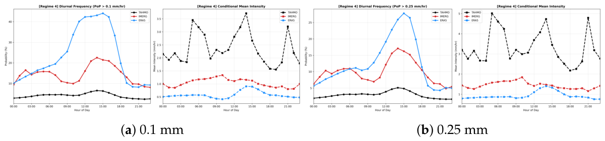
At the threshold of mm/hr, ERA5 exhibits a massive overestimation of rainfall frequency, reaching a PoP of 35% at 16:00 LST. In contrast, TAHMO hovers below 7% while IMERG remains below a 22% probability of occurrence at this threshold. However, when evaluating the Conditional Mean Intensity of these wet hours, TAHMO dominates. TAHMO registers sharp, high-magnitude spikes (e.g., 4.3 mm/hr and 5mm/hr at 08:00 LST and 12:00 LST respectively, and multiple nocturnal bursts mm/hr), whereas ERA5’s conditional intensity rarely exceeds 1.1 mm/hr, as shown in Figure 10.
This inverse relationship—where ERA5 generates rainfall almost half the time but at highly suppressed magnitudes—confirms a “drizzle bias” inherent to its convective parameterisation scheme. It satisfies its daily volumetric water budget through persistent, light rain rather than resolving the discrete, violent mesoscale convective systems captured by the gauges.
An exhaustive breakdown of PoP and conditional intensities across certain physical thresholds and across the regimes is provided in Appendix A.
3.4.4. Percentiles of the Diurnal Cycle
The percentile analysis further validates the discrete nature of East African convection. As shown in Figure 11, across all regions, the median state () for TAHMO and IMERG is completely dry (0.0 mm/hr), physically reflecting that rain does not occur on the majority of days at any given hour. ERA5, on the other hand, registers precipitation (trace rain) even at the 50th percentile, further exposing its over-triggering. The true convective signals for TAHMO and IMERG only emerge in the upper percentiles ( to ), showing that regional precipitation is driven by rare, heavy-tail events rather than central-tendency means.
Percentiles of each regime are provided in Appendix A.
4. Discussion
4.1. Overcoming Spatial and Distributional Mismatches
The foundational step of our analysis highlighted a penalty of spatial support mismatch between areal and point-scale datasets as shown in the systematic correlation improvement achieved via bilinear interpolation (Table 2).
However, addressing spatial scale alone is insufficient due to the zero-inflated, heavy-tailed nature of precipitation. The transition into transformed spaces (Box-Cox and ArcSinh) proved critical (Table 4). By compressing extreme right-tail outliers, these transformations force the evaluation metrics to prioritise the event detection of rain vs. no-rain rather than being overwhelmingly skewed by a single extreme event.
Practically, this revealed that GPPs possess fundamentally different underlying distributions. The performance of Box-Cox when applied to CHIRPS and TAMSAT demonstrates that they produce “hard zeros” which are distorted by aggressive power transforms. On the other hand, ERA5 and IMERG require the specific parameterisation of Box-Cox to effectively stretch the boundary between dry days and their inherent trace-level noise. For hydrologists and machine learning practitioners, this indicates that applying a uniform statistical transformation across different precipitation products will inherently degrade the signals of some while enhancing others; transformation strategies must be dynamically tailored to the dataset’s specific climatological behavior.
4.2. The Physical Basis for Shifting Temporal Alignment
The comparison between static uniform shifting and 30-day rolling-window analysis proved that temporal displacement in GPPs is non-stationary. As demonstrated in Table 5, while the median shift across the datasets is 0.0 days, the standard deviations approximate to days. This indicates that phase mismatch is highly dependent on localised weather systems rather than a systematic global delay.
The findings from the hourly diurnal analysis provide the fundamental physical explanation for this daily-scale stochasticity. The diurnal phase analysis revealed that actual precipitation exhibits complex, multi-modal timing dictated by local topography as shown by the phase peaks and how the GPPs’ peaks align to TAHMO’s peaks in Table 7.
4.3. Diagnosing Parameterisation Flaws
By evaluating the datasets in an optimised transformed space, we were able to rank the GPPs based on their true physical accuracy (Table 6). While IMERG demonstrated superior correlation and volume accuracy (), the ranking analysis exposed a performance paradox within ERA5. Despite achieving the second-highest optimal correlation (), ERA5 registered the lowest Bias Score () of all datasets. The diurnal cycle analysis definitively explains this paradox. At the hourly scale at a 0.1 mm/hr threshold, ERA5 exhibits a massive Probability of Precipitation (PoP of 35% at 16:00 LST), yet its Conditional Mean Intensity rarely exceeds 1.1 mm/hr. In contrast, TAHMO rains much less frequently but at highly concentrated, intense magnitudes (e.g., bursts mm/hr) Figure 10.
In our daily-scale methodology, the conditional Bias Score utilises an exclusion logic that removes “State mismatches”—instances where one dataset records a dry state and the other records a wet state. ERA5’s low Bias Score exposes its “drizzle bias.” Because it frequently reports low-intensity precipitation during physically dry periods, forcing persistent state mismatches with TAHMO. ERA5 satisfies its total daily volumetric budget by drizzling lightly across the entire day.
4.4. Event Detection and Accuracy
IMERG demonstrated superior overall timing and volume accuracy. This conclusion strongly aligns with recent regional evaluations utilising the TAHMO network [34], who similarly identified IMERG as more reliable when compared to datasets like CHIRPS and ERA5. At the daily scale, IMERG and ERA5 achieved the highest rain event detection skill—answering the question, `Did it rain today?’—yielding point-to-point CSI scores of 0.3481 and 0.3068, respectively. On the other hand, CHIRPS and TAMSAT have lower detection skill with point-to-point CSI of 0.2914 and 0.2898, respectively, indicating a much higher rate of missed events and false alarms. The variance scores further highlight the performance of CHIRPS and TAMSAT, where lower values indicate a failure to capture the variability of rainfall. While IMERG and ERA5 show higher variance scores (0.8581 and 0.8145 respectively), CHIRPS and TAMSAT have lower scores of 0.6874 and 0.6958 (Table 6). Previous studies utilising the TAHMO network [20] have established that CHIRPS suffers from volumetric overestimations in East Africa using traditional raw-space metrics. Our variance-stabilised analysis builds upon this by revealing that CHIRPS does not simply overestimate rainfall amounts; it exhibits poor rain event detection and does not align them in time as well as IMERG or ERA5.
Furthermore, isolating the geometric mean of the bias () and variability ratios () within the transformed space shows how this failure happens. As shown in Table 6, CHIRPS registers a geometric mean bias ratio of 1.8551 combined with a high geometric mean variability ratio of 1.6933 in the transformed space. Because the ArcSinh transformation actively compresses extreme right-tail outliers, this overestimation of the geometric mean suggests that the regional wet bias in CHIRPS is driven by systematic over-estimation of the typical state of day-to-day precipitation while producing spurious fluctuations between wet and dry states.
Operational Implications
Distinguishing between detection skill and volumetric accuracy carries profound implications for operational hydrology and climate downscaling in East Africa. The high event detection scores achieved by IMERG and ERA5 indicate that their internal parameterisations are highly optimised for occurrence-based applications. For tasks such as agricultural drought monitoring, crop-yield forecasting, and categorical anomaly detection, successfully capturing the duration of dry spells or the exact frequency of wet days is fundamentally more critical than estimating absolute rainfall intensity. In these contexts, both datasets provide highly robust utility.
Beyond basic event detection, impact models requiring strict mass conservation and dynamic phase accuracy—such as river routing, flash flood forecasting, and fine-scale atmospheric downscaling—demand rigorous volumetric precision. In these volume-dependent applications, relying on datasets with much lower detection skill such as CHIRPS and TAMSAT introduces substantial risk. IMERG maintains high detection skill while simultaneously preserving the heavy-tailed variance and the central tendency of the physical water budget, thus emerging as the optimal choice for these specific tasks.
5. Conclusion
This study demonstrates that evaluating GPPs in East Africa requires moving beyond traditional raw-space, static comparisons. Due to the heavy-tailed, zero-inflated nature of precipitation and the spatial support mismatch between point-scale gauges and areal grids, applying dataset-specific variance-stabilising transformations (Box-Cox and ArcSinh) is useful in finding spatial and timing patterns. Furthermore, our diurnal phase analysis revealed that temporal mismatches between GPPs and ground observations are not systematic global delays, but rather random artifacts driven by local topography and convective parameterisations.
By isolating timing accuracy from volume accuracy, our analysis reveals that each GPP should be utilised based on its strengths. IMERG achieved the highest overall timing and volume accuracy, establishing it as suitable for volume-dependent tasks like flash flood modeling. Meanwhile, despite exhibiting high baseline correlations, ERA5 is characterised by a drizzle bias. It satisfies its diurnal water budget through persistent, low-intensity drizzle while failing to capture the intense, discrete convective bursts that characterise East African hydroclimatology.
These findings carry implications for regional climate impact studies and the development of AI-driven weather emulators. First, utilising raw GPPs, especially ERA5 precipitation directly for local hydrological modelling without bias correction or post-processing is highly discouraged. Second, when training machine learning downscaling models, developers should consider how they evaluate the models. Standard evaluation metrics like RMSE rely on strict point-to-point comparisons, meaning they heavily penalise minor timing errors. If a model accurately simulates a rain event but places it two hours early, RMSE punishes it twice: once for a false alarm, and once for the missed event. These models should instead be rewarded for predicting the timing, volume and intensity of localised rain events.
Author Contributions
Conceptualisation, T.L. and [C.W.]; methodology, T.L.; software, T.L.; formal analysis, T.L.; investigation, T.L.; resources, [C.W.]; writing—original draft preparation, T.L.; writing—review and editing, [C.W.]; visualisation, T.L.; supervision, [C.W.]; project administration, [C.W.]; funding acquisition, [C.W.]. All authors have read and agreed to the published version of the manuscript.
Funding
This work was supported by the Artificial Intelligence for Development (AI4D) program, with the financial support of the UK government’s Foreign, Commonwealth, and Development Office (FCDO) and Canada’s International Development Research Centre (IDRC). This work was also supported in part by the Gates Foundation [INV-079120]. The conclusions and opinions expressed in this work are those of the author(s) alone and shall not be attributed to the Foundation. We also acknowledge support to DSAIL from Arm and Google.org. In addition, this work obtained computational resources from the Swiss National Supercomputing Centre (CSCS) under project ID g164 on Alps.
Data Availability Statement
The datasets analyzed during this study are derived from a combination of public repositories and restricted-access networks. ERA5 reanalysis data are available through the Copernicus Climate Data Store (CDS). CHIRPS precipitation data can be accessed and downloaded via Google Earth Engine (GEE). TAMSAT precipitation estimates are accessible via the official TAMSAT API. Ground observation data from the Trans-African Hydro-Meteorological Observatory (TAHMO) are available via the TAHMO API; however, access is restricted and requires a formal data request and approval from the TAHMO administration.
Acknowledgments
We thank the Trans-African Hydro-Meteorological Observatory (TAHMO) for access to ground observation data from their network of weather stations. The authors would like to thank Professors John Selker and Thomas Dietterich for useful discussions and suggestions. In preparing this manuscript, the author utilised Gemini 3 Pro to assist with code debugging.
Conflicts of Interest
“The funders had no role in the design of the study; in the collection, analyses, or interpretation of data; in the writing of the manuscript; or in the decision to publish the results”.
Abbreviations
The following abbreviations are used in this manuscript:
| GPP | Gridded Precipitation Product |
| KGE | Kling-Gupta Efficiency |
| CSI | Critical Success Index |
| QC | Quality Control |
| PoP | Probability of Precipitation |
| TIR | Thermal Infrared |
| MW | Microwave |
| IR | Infrared |
| LST | Local Standard Time (Coordinated Universal Time +3) |
| OND | October-November-December |
| MAM | March-April-May |
| BIC | Bayesian Information Criterion |
| PCA | Principal Component Analysis |
| GMM | Gaussian Mixture Model |
Appendix A
Appendix A.1. Spatial Support Mismatch and the Normalisation Artifact
As illustrated in the domain-wide evaluation (Figure 8), a distinct “order flip” occurs between the raw intensity and the normalised phase profiles during the early morning hours (e.g., 01:00 to 04:00 LST). In the absolute intensity space, the TAHMO gauge network records higher physical precipitation volumes than the IMERG satellite product. However, when transitioning to the Min-Max normalised in the transformed space, this hierarchy inverts, and IMERG appears to exhibit a much stronger relative morning phase than TAHMO.
This phenomenon is not an error in the observational data, but rather a direct mathematical consequence of spatial support mismatch. The phase normalisation maps the diurnal cycle to a scale by dividing the hourly intensities by the total diurnal amplitude ().
As demonstrated by Peleg et al. [35] , point-scale gauges inherently capture the extreme, highly localised cores of convective rain. When it rains over a TAHMO station, the gauge registers a massive, unsmoothed afternoon peak, resulting in an exceptionally large denominator. In contrast, areal gridded products like IMERG (representing a roughly km pixel on the ground) spatially average these sub-grid convective cores with the surrounding non-precipitating areas, artificially dampening their diurnal maximum.
Because TAHMO’s normalisation denominator is physically much larger, its non-peak nocturnal hours are compressed toward zero. IMERG, possessing a dampened afternoon peak and thus a smaller diurnal range, allocates a larger percentage of its total daily variance to the morning hours.
Therefore, the observed “flip” in Figure 8 does not outrightly indicate that IMERG measures more morning rain; rather, it highlights the spatial variance penalty.
Appendix A.2. Regime-Level Probabiliy of Precipitation and Conditional Mean Intensity
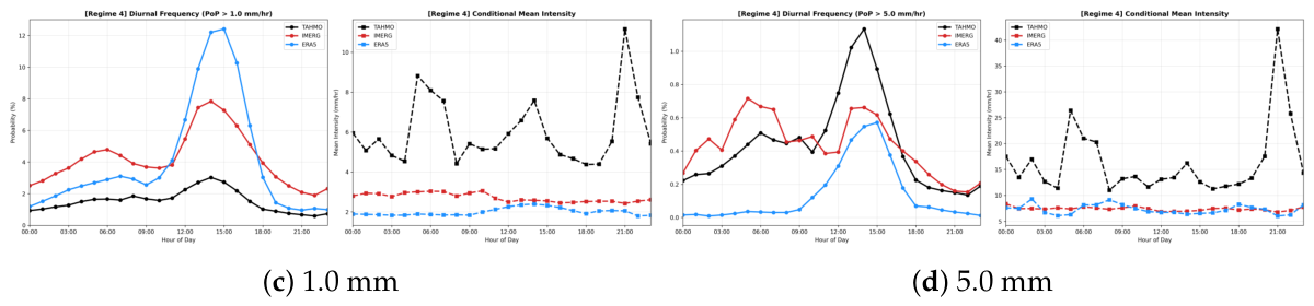
The figures below highlight the diurnal cycle considered at different precipitation thresholds for the various regimes.
Figure A1 below shows the probability of precipitation and conditional mean intensity for regime 0.
Figure A1.
Regime 0 diurnal cycle PoP and mean intensity at various precipitation thresholds.
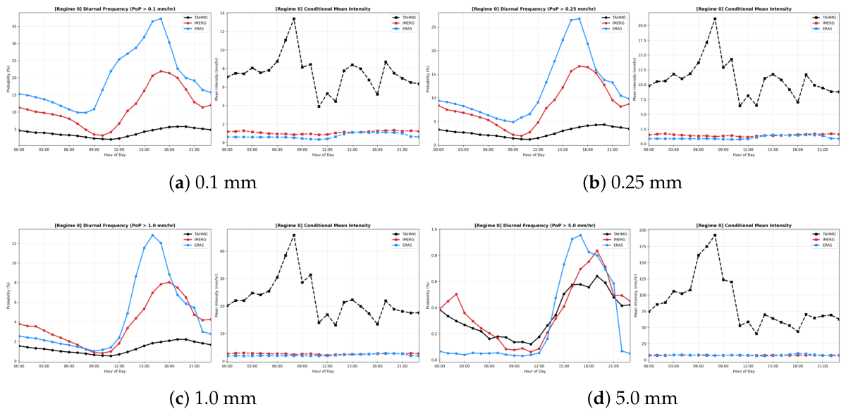
Figure A2 below shows the probability of precipitation and conditional mean intensity for regime 1.
Figure A2.
Regime 1 diurnal cycle PoP and mean intensity at various precipitation thresholds.
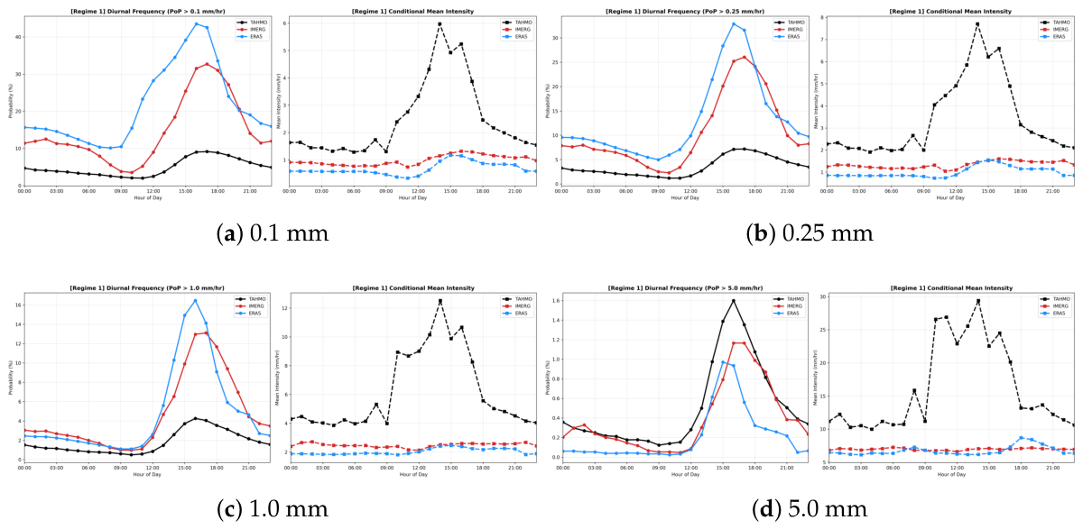
Figure A3 below shows the probability of precipitation and conditional mean intensity for regime 2.
Figure A3.
Regime 2 diurnal cycle PoP and mean intensity at various precipitation thresholds.
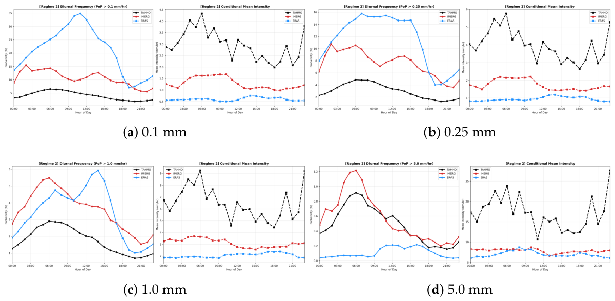
Figure A4 below shows the probability of precipitation and conditional mean intensity for regime 3.
Figure A4.
Regime 3 diurnal cycle PoP and mean intensity at various precipitation thresholds.
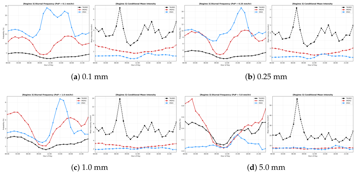
Figure A5 below shows the probability of precipitation and conditional mean intensity for regime 4.
Figure A5.
Regime 4 diurnal cycle PoP and mean intensity at various precipitation thresholds.
Appendix A.3. Seasonal Diurnal Cycle at Each Regime
The results shown in Figure A6 are those of Timing and Volume in Section 2.5.2 where we look at the mean diurnal cycle at seasonal levels. It is also influenced by the normalisation in Appendix A.1, in the transformed space.
Figure A6.
Seasonal diurnal cycle phase alignment analysis in all the regimes.
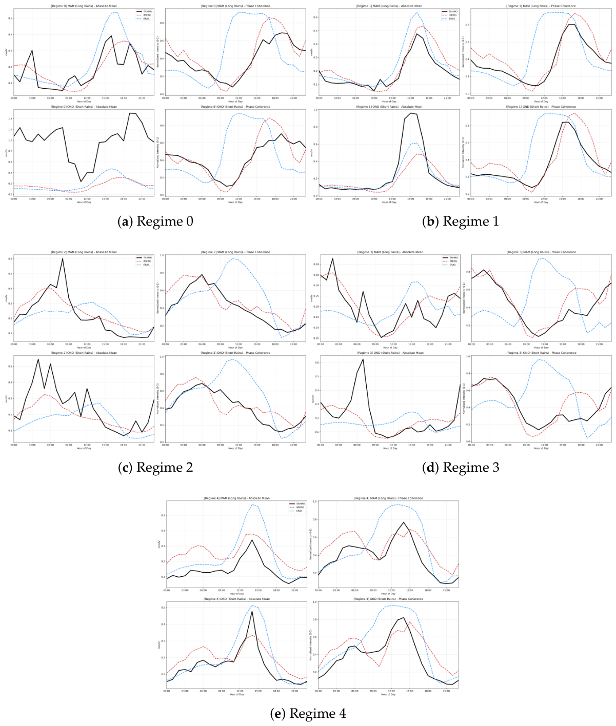
The results indicate that the 19:00 LST in Regime 0’s mean diurnal cycle is largely as a result of the October-November-December short rains season.
It also shows that even within the regimes, there is a difference in the precipitation experienced in different seasons. For instance, in Regime 0, the absolute mean intensity during OND is on average greater than that of MAM, using TAHMO as our reference.
Appendix A.4. Diurnal Cycle Percentiles
This section shows the results of the percentile analysis at each regime.
Figure A7.
Sub-regional percentiles of the diurnal cycle.
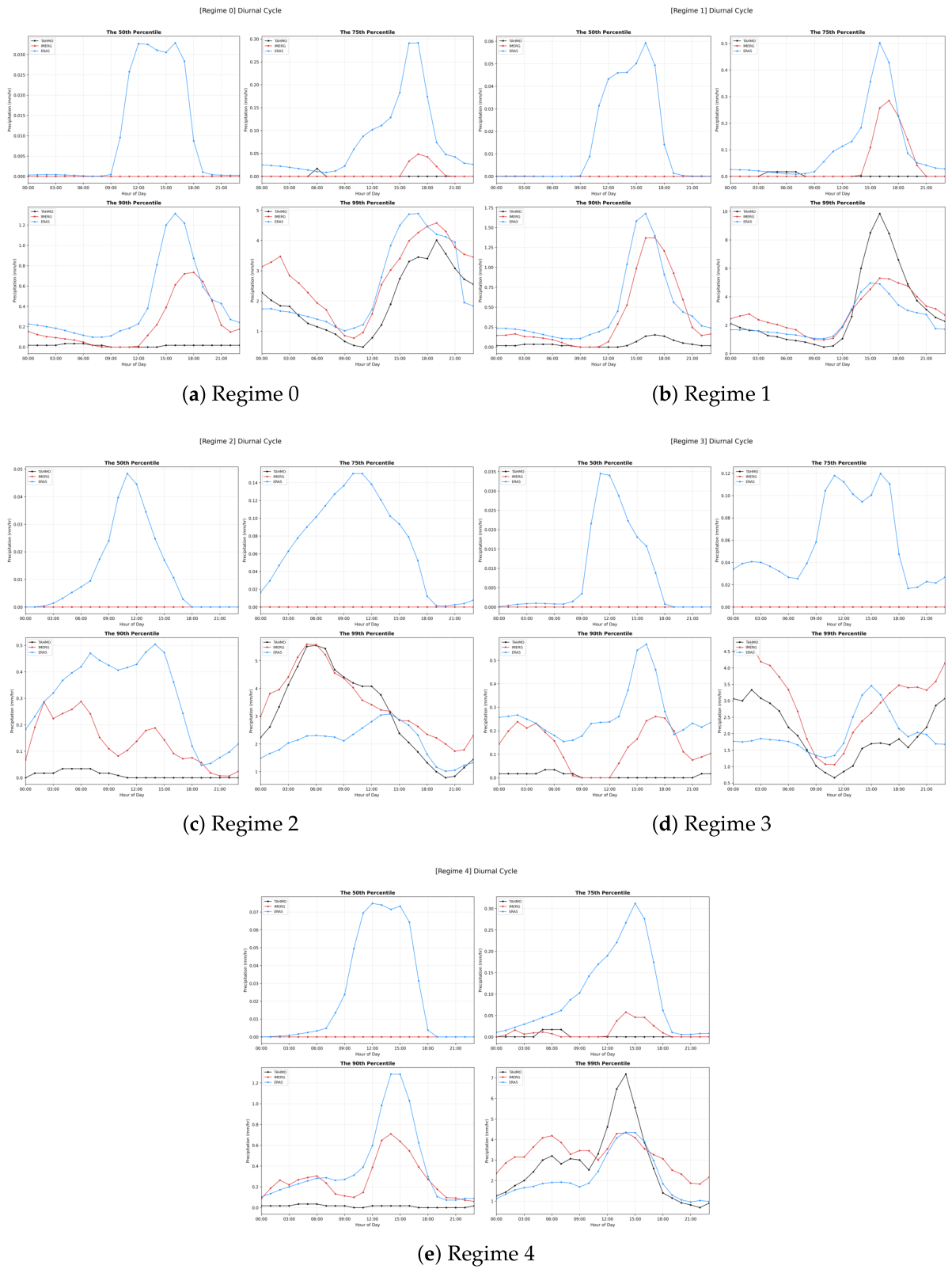
The median state even at the regime level shows the ERA5 “drizzle bias” in all the regimes as shown by Figure A7.
References
- Dinku, T.; Ceccato, P.; Grover-Kopec, E.; Lemma, M.; Connor, S.J.; Ropelewski, C.F. Validation of satellite rainfall products over East Africa’s complex topography. In International Journal of Remote Sensing; Taylor & Francis _eprint, 2007; Volume 28, pp. 1503–1526. [Google Scholar] [CrossRef]
- Opere, A. Floods in Kenya. In Developments in Earth Surface Processes; Elsevier, 2013; Vol. 16, pp. 315–330. [Google Scholar] [CrossRef]
- Marchant, R.; Mumbi, C.; Behera, S.; Yamagata, T. The Indian Ocean dipole – the unsung driver of climatic variability in East Africa. Afr. J. Ecol. 2007, 45, 4–16. [Google Scholar] [CrossRef]
- Washington, R.; Harrison, M.; Conway, D.; Black, E.; Challinor, A.; Grimes, D.; Jones, R.; Morse, A.; Kay, G.; Todd, M. African climate change: taking the shorter route. Bull. Am. Meteorol. Soc. 2006, 87, 1355–1366. [Google Scholar] [CrossRef]
- Huffman, G.J.; Bolvin, D.T.; Braithwaite, D.; Hsu, K.L.; Joyce, R.J.; Kidd, C.; Nelkin, E.J.; Sorooshian, S.; Stocker, E.F.; Tan, J.; et al. Integrated Multi-satellite Retrievals for the Global Precipitation Measurement (GPM) Mission (IMERG). In Satellite Precipitation Measurement; Levizzani, V., Kidd, C., Kirschbaum, D.B., Kummerow, C.D., Nakamura, K., Turk, F.J., Eds.; Springer International Publishing: Cham, 2020; Volume 1, pp. 343–353. [Google Scholar] [CrossRef]
- Funk, C.; Peterson, P.; Landsfeld, M.; Pedreros, D.; Verdin, J.; Shukla, S.; Husak, G.; Rowland, J.; Harrison, L.; Hoell, A.; et al. The climate hazards infrared precipitation with stations—a new environmental record for monitoring extremes. In Scientific Data; Springer Science and Business Media LLC: Publisher, 2015; p. 2. [Google Scholar] [CrossRef] [PubMed]
- Hersbach, H.; Bell, B.; Berrisford, P.; Hirahara, S.; Horányi, A.; Muñoz-Sabater, J.; Nicolas, J.; Peubey, C.; Radu, R.; Schepers, D.; et al. The ERA5 global reanalysis. Q. J. R. Meteorol. Soc. 2020, 146, 1999–2049. [Google Scholar] [CrossRef]
- Sun, Q.; Miao, C.; Duan, Q.; Ashouri, H.; Sorooshian, S.; Hsu, K.L. A Review of Global Precipitation Data Sets: Data Sources, Estimation, and Intercomparisons. Rev. Geophys. 2018, 56, 79–107. [Google Scholar] [CrossRef]
- Xiang, Y.; Chen, J.; Li, L.; Peng, T.; Yin, Z. Evaluation of Eight Global Precipitation Datasets in Hydrological Modeling. In Remote Sensing; Multidisciplinary Digital Publishing Institute, 2021; Volume 13. [Google Scholar] [CrossRef]
- Kling, H.; Fuchs, M.; Paulin, M. Runoff conditions in the upper Danube basin under an ensemble of climate change scenarios. J. Hydrol. 2012, 424-425, 264–277. [Google Scholar] [CrossRef]
- Lavers, D.A.; Hersbach, H.; Rodwell, M.J.; Simmons, A. An improved estimate of daily precipitation from the ERA5 reanalysis. Atmos. Sci. Lett. 2024, 25, e1200. _eprint. Available online: https://rmets.onlinelibrary.wiley.com/doi/pdf/10.1002/asl.1200. [CrossRef]
- Gleixner, S.; Demissie, T.; Diro, G.T. Did ERA5 Improve Temperature and Precipitation Reanalysis over East Africa? In Atmosphere; Multidisciplinary Digital Publishing Institute, 2020; Volume 11. [Google Scholar] [CrossRef]
- Lazoglou, G.; Economou, T.; Anagnostopoulou, C.; Zittis, G.; Tzyrkalli, A.; Georgiades, P.; Lelieveld, J. Multivariate adjustment of drizzle bias using machine learning in European climate projections. 2024. [Google Scholar] [CrossRef]
- Beck, H.; McVicar, T.; van Dijk, A.; Schellekens, J.; de Jeu, R.; Bruijnzeel, L. Global evaluation of four AVHRR–NDVI data sets: Intercomparison and assessment against Landsat imagery. Remote Sens. Environ. 2011, 115, 2547–2563. [Google Scholar] [CrossRef]
- Davis, C.; Brown, B.; Bullock, R. Object-Based Verification of Precipitation Forecasts. Part I: Methodology and Application to Mesoscale Rain Areas. Mon. Weather Rev. 2006, 134, 1772–1784. [Google Scholar] [CrossRef]
- Ebert, E.E. Fuzzy verification of high-resolution gridded forecasts: a review and proposed framework. Meteorol. Appl. 2008, 15, 51–64. [Google Scholar] [CrossRef]
- Davis, C.; Brown, B.; Bullock, R. Object-Based Verification of Precipitation Forecasts. Part II: Application to Convective Rain Systems. Mon. Weather Rev. 2006, 134, 1785–1795. [Google Scholar] [CrossRef]
- Hayden, L.J.M.; Tan, J.; Bolvin, D.T.; Huffman, G.J. Variations in the Diurnal Cycle of Precipitation and Its Changes with Distance from Shore over Two Contrasting Regions as Observed by IMERG, ERA5, and Spaceborne Ku Radar. J. Hydrometeorol. 2023, 24, 675–689. [Google Scholar] [CrossRef]
- van de Giesen, N.; Hut, R.; Selker, J. The trans-African hydro-meteorological observatory (TAHMO). In Wiley Interdisciplinary Reviews: Water; 2014; Volume 1, pp. 341–348. [Google Scholar]
- Macharia, D.; Fankhauser, K.; Selker, J.S.; Neff, J.C.; Thomas, E.A. Validation and Intercomparison of Satellite-Based Rainfall Products over Africa with TAHMO In Situ Rainfall Observations. In Journal of Hydrometeorology; American Meteorological Society Section: Journal of Hydrometeorology, 2022; Volume 23, pp. 1131–1154. [Google Scholar] [CrossRef]
- Wang, Q.J.; Shrestha, D.L.; Robertson, D.E.; Pokhrel, P. A log-sinh transformation for data normalization and variance stabilization. Water Resour. Res. 2012, 48, 2011WR010973. [Google Scholar] [CrossRef]
- Burbidge, J.B.; Magee, L.; Robb, A.L. Alternative Transformations to Handle Extreme Values of the Dependent Variable. J. Am. Stat. Assoc. 1988, 83, 123–127. [Google Scholar] [CrossRef]
- Quintero, F.; Mantilla, R.; Anderson, C.; Claman, D.; Krajewski, W. Assessment of Changes in Flood Frequency Due to the Effects of Climate Change: Implications for Engineering Design. In Hydrology; Multidisciplinary Digital Publishing Institute, 2018; Volume 5. [Google Scholar] [CrossRef]
- Najafi, H.; Lagerwall, G.L.; Obeysekera, J.; Liu, J. Machine Learning in Climate Downscaling: A Critical Review of Methodologies, Physical Consistency, and Operational Applications. In Water; Multidisciplinary Digital Publishing Institute: Publisher, 2026; Volume 18. [Google Scholar] [CrossRef]
- Nicholson, S.E.; Hartman, A.T.; Klotter, D.A. On the diurnal cycle of rainfall and convection over Lake Victoria and its catchment. Part 1: Rainfall and Mesoscale Convective Systems. J. Hydrometeorol. 2021. [Google Scholar] [CrossRef]
- Camberlin, P.; Gitau, W.; Planchon, O.; Dubreuil, V.; Funatsu, B.M.; Philippon, N. Major role of water bodies on diurnal precipitation regimes in Eastern Africa _eprint. Int. J. Climatol. 2018, 38, 613–629. Available online: https://rmets.onlinelibrary.wiley.com/doi/pdf/10.1002/joc.5197. [CrossRef]
- Maidment, R.; Black, E.; Greatrex, H.; Young, M. TAMSAT. In Satellite Precipitation Measurement; Levizzani, V., Kidd, C., Kirschbaum, D.B., Kummerow, C.D., Nakamura, K., Turk, F.J., Eds.; Springer International Publishing: Cham, 2020; Volume 1, pp. 393–408. [Google Scholar] [CrossRef]
- Box, G.E.P.; Cox, D.R. An Analysis of Transformations. J. R. Stat. Soc. Ser. B Stat. Methodol. 1964, 26, 211–243. [Google Scholar] [CrossRef]
- Schaefer, J.T. The Critical Success Index as an Indicator of Warning Skill. In Weather and Forecasting;Section: Weather and Forecasting; 1990. [Google Scholar]
- Maraun, D.; Shepherd, T.G.; Widmann, M.; Zappa, G.; Walton, D.; Gutiérrez, J.M.; Hagemann, S.; Richter, I.; Soares, P.M.M.; Hall, A.; et al. Towards process-informed bias correction of climate change simulations. In Nature Climate Change; Nature Publishing Group: Publisher, 2017; Volume 7, pp. 764–773. [Google Scholar] [CrossRef]
- Wilks, D.S. Statistical Methods in the Atmospheric Sciences; Academic Press, 2011. [Google Scholar]
- Hill, P.G.; Stein, T.H.M.; Cafaro, C. Convective systems and rainfall in East Africa _eprint. Q. J. R. Meteorol. Soc. 2023, 149, 2943–2961. Available online: https://rmets.onlinelibrary.wiley.com/doi/pdf/10.1002/qj.4540. [CrossRef]
- Limbu, P.T.; King’uza, P.H.; Okrah, A. Characteristics of the observed diurnal cycle of precipitation during long-rain season over Tanzania. Theor. Appl. Climatol. 2026, 157, 301. [Google Scholar] [CrossRef]
- Hoogelander, V.; Hut, R.; Coz, C.L.; Dong, J.; Giesen, N.v.d. Enhancing Rainfall Estimates in East Africa by Integrating TAHMO Ground Data and Satellite Rainfall Products. In Journal of Hydrometeorology; American Meteorological Society Section: Journal of Hydrometeorology, 2025; Volume 26, pp. 1063–1087. [Google Scholar] [CrossRef]
- Peleg, N.; Marra, F.; Fatichi, S.; Paschalis, A.; Molnar, P.; Burlando, P. Spatial variability of extreme rainfall at radar subpixel scale. J. Hydrol. 2018, 556, 922–933. [Google Scholar] [CrossRef]
Figure 1.
Overview of the East African study area showing the locations of the TAHMO ground station network in the region.
Figure 1.
Overview of the East African study area showing the locations of the TAHMO ground station network in the region.
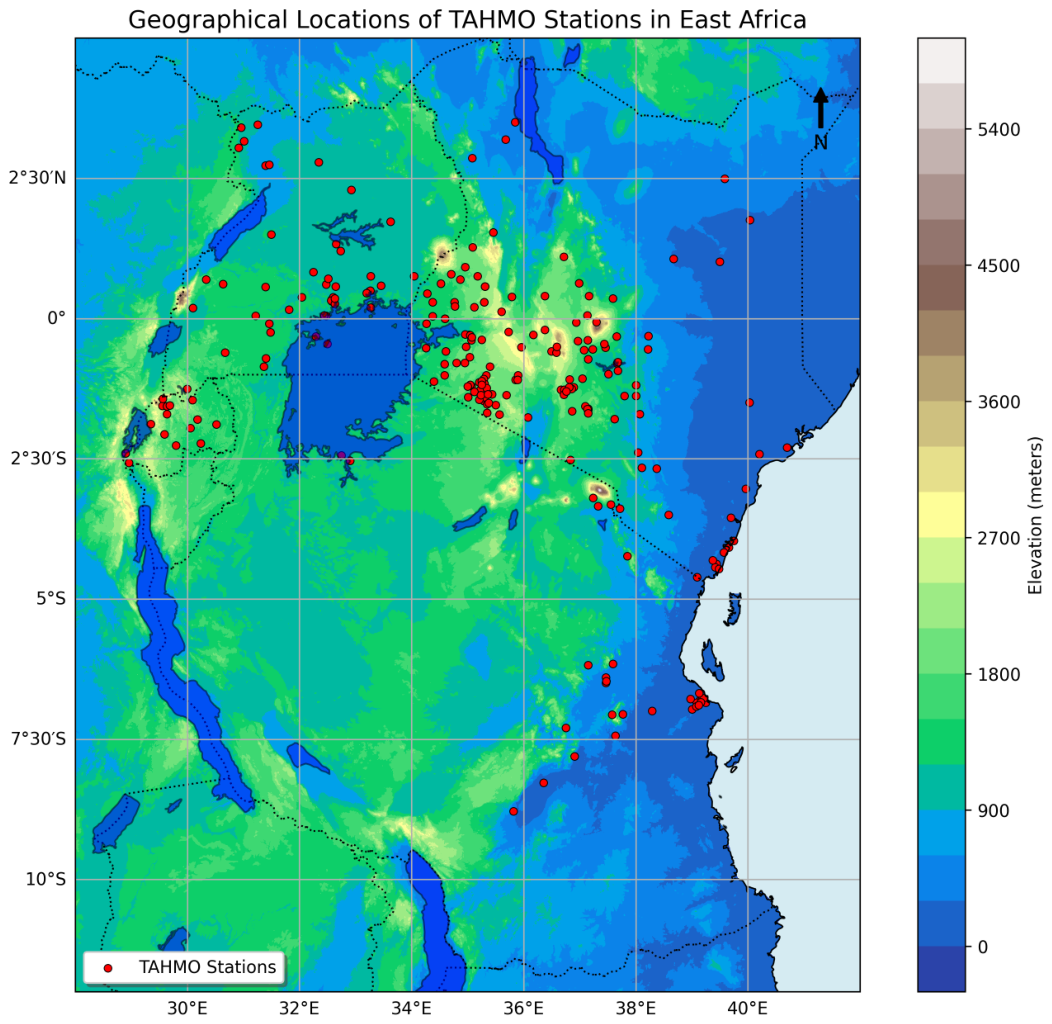
Figure 2.
Smoothing Kernel width performance using kernel width values ranging from 0 to 21 days.
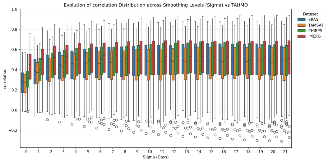
Figure 3.
Correlation comparison at of the Original signals, Box-Cox and ArcSinh transformations.
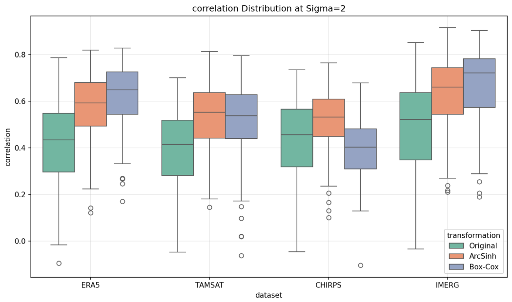
Figure 4.
Shifting and smoothing result example comparing IMERG and TAHMO for the period March - May (MAM) 2024, here the optimal shift was 0 days.
Figure 4.
Shifting and smoothing result example comparing IMERG and TAHMO for the period March - May (MAM) 2024, here the optimal shift was 0 days.
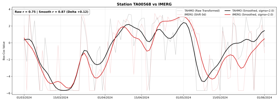
Figure 5.
Shifting and smoothing results comparing IMERG and ERA5 at TA00283, which shows the difference between these two GPPs at this station.
Figure 5.
Shifting and smoothing results comparing IMERG and ERA5 at TA00283, which shows the difference between these two GPPs at this station.
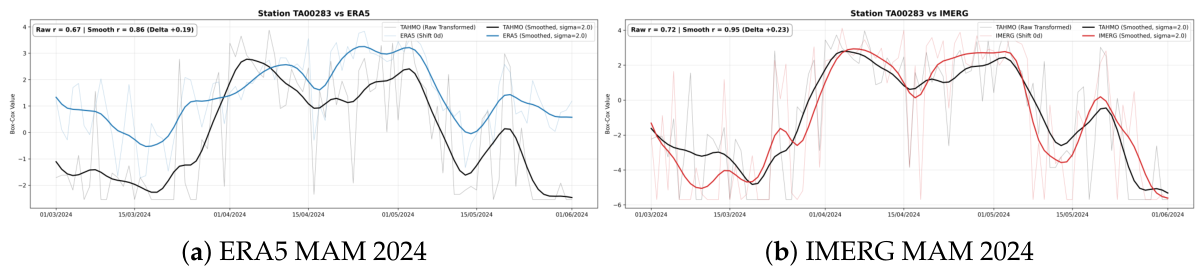
Figure 6.
Shift distribution of the optimal lags [-3, +3] across the study area.
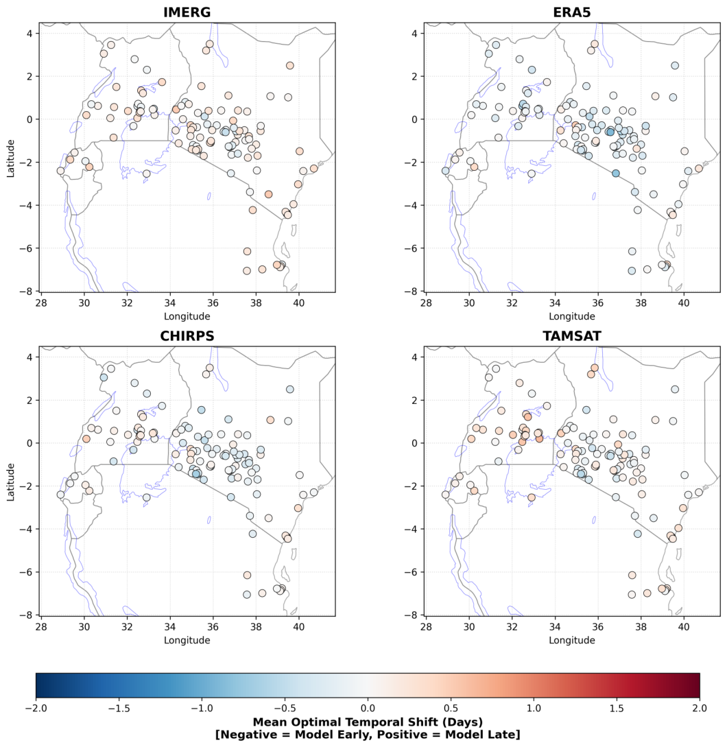
Figure 7.
Diurnal cycle regimes peaks and spatial distribution across the region for TAHMO, IMERG and ERA5.
Figure 7.
Diurnal cycle regimes peaks and spatial distribution across the region for TAHMO, IMERG and ERA5.
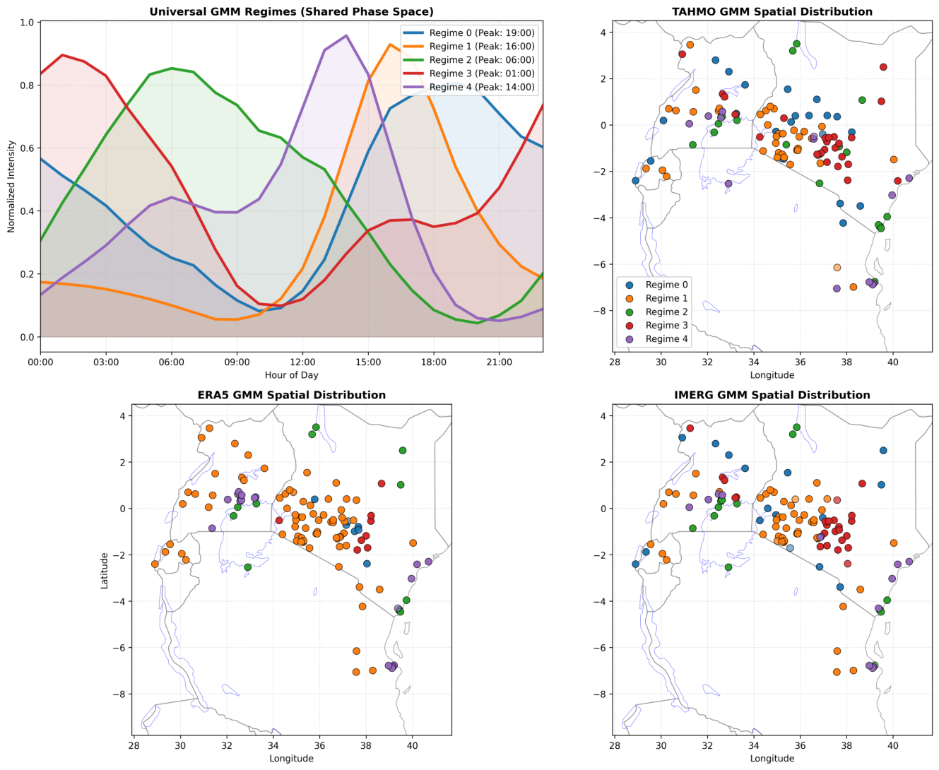
Figure 8.
East Africa regional volume and phase analysis.
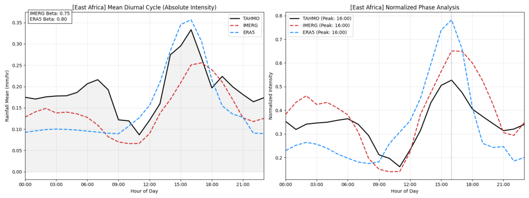
Figure 9.
Regional diurnal cycle analysis (absolute volume and normalised phase). The decomposition into 5 regimes reveals significant spatial heterogeneity
Figure 9.
Regional diurnal cycle analysis (absolute volume and normalised phase). The decomposition into 5 regimes reveals significant spatial heterogeneity
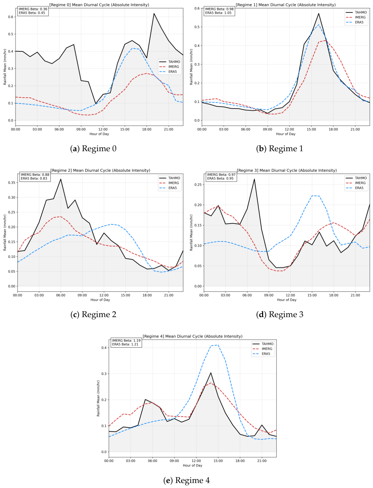
Figure 10.
Diurnal Probability of Precipitation (PoP) and Conditional Mean Intensity evaluated across varying physical thresholds. Lower thresholds (0.05 to 0.25 mm/hr) expose the persistent, low-intensity drizzle bias in ERA5, while higher thresholds (2.5 and 5.0 mm/hr) demonstrate the concentration of actual precipitation volume within rare, extreme mesoscale convective bursts captured by TAHMO.
Figure 10.
Diurnal Probability of Precipitation (PoP) and Conditional Mean Intensity evaluated across varying physical thresholds. Lower thresholds (0.05 to 0.25 mm/hr) expose the persistent, low-intensity drizzle bias in ERA5, while higher thresholds (2.5 and 5.0 mm/hr) demonstrate the concentration of actual precipitation volume within rare, extreme mesoscale convective bursts captured by TAHMO.
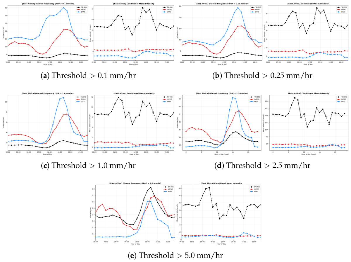
Figure 11.
Percentile analysis of the East African domain, showing ERA5 has a “drizzle bias” around the median state (50th percentile) and in the 75th percentile.
Figure 11.
Percentile analysis of the East African domain, showing ERA5 has a “drizzle bias” around the median state (50th percentile) and in the 75th percentile.
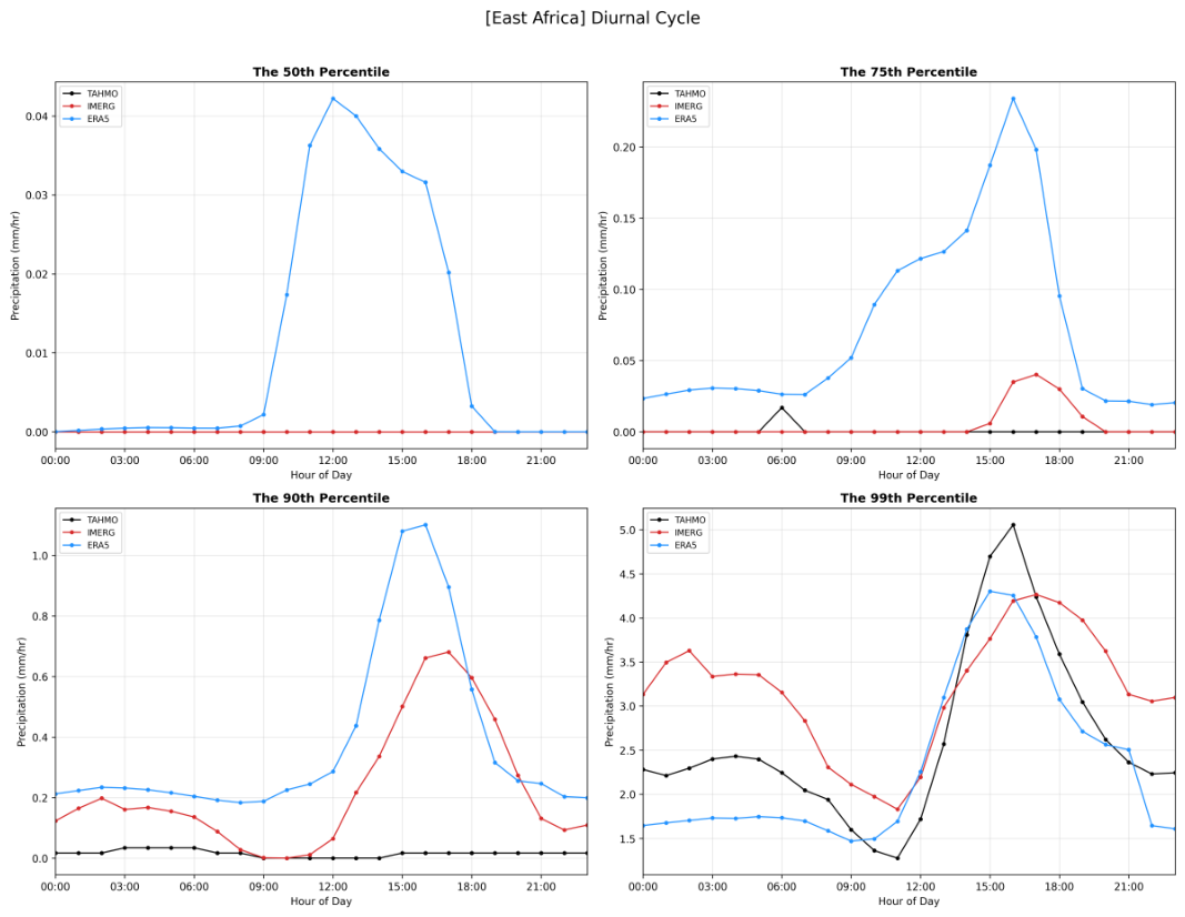

Table 1.
Characteristics of the gridded precipitation products used in this study.
| Dataset | Type | Spatial Resolution | Temporal Resolution | Reference |
|---|---|---|---|---|
| ERA5 | Reanalysis | Hourly | [7] | |
| IMERG V07 Final | Satellite (MW/IR) | 30-min | [5] | |
| TAMSAT v3.1 | Satellite (TIR) | Daily | [27] | |
| CHIRPS v2.0 | Blended | Daily | [6] |
Table 2.
Mean Correlation Improvement using Bilinear Interpolation over Nearest Neighbour.
| Dataset | (Improvement) |
|---|---|
| IMERG | |
| ERA5 | |
| CHIRPS | |
| TAMSAT |
Table 3.
Optimised Box-Cox Parameters for daily-scale via Skewness Minimisation.
| Dataset | Offset () | Lambda () |
|---|---|---|
| ERA5 | 0.0800 | -0.005 |
| IMERG | 0.0030 | 0.007 |
| TAMSAT | 0.0001 | -0.196 |
| CHIRPS | 0.0001 | -2.202 |
Table 4.
Mean Correlation by Transformation Method ().
| Transformation | Average Correlation (r) |
|---|---|
| ArcSinh | 0.5658 |
| Box-Cox | 0.5509 |
| Original (Raw) | 0.4288 |
Table 5.
Shift Dynamics and Baseline Correlation Improvements at the Daily Scale.
| Dataset | Mean Shift (days) | Median (days) | Std. Dev. (days) | |||
|---|---|---|---|---|---|---|
| IMERG | 0.0 | 1.703 | 0.5635 | 0.6711 | ||
| ERA5 | 0.0 | 1.837 | 0.5140 | 0.6316 | ||
| TAMSAT | 0.0 | 1.960 | 0.4037 | 0.5622 | ||
| CHIRPS | 0.0 | 1.995 | 0.4014 | 0.5580 |
Table 6.
Daily Scale Evaluation Metrics and Composite Ranking in Transformed Space.
| Dataset | Comp. Score | Opt. r | Fuzzy CSI | Point CSI | Bias Score | Variance Score | Consistency | Improvement | ||
|---|---|---|---|---|---|---|---|---|---|---|
| IMERG | 0.6059 | 0.6701 | 0.4942 | 0.3481 | 0.7267 | 0.8581 | 0.9052 | 1.0514 | 0.7721 | 0.1084 |
| ERA5 | 0.5729 | 0.6306 | 0.4778 | 0.3068 | 0.6389 | 0.8145 | 0.7929 | 1.1609 | 0.7661 | 0.1181 |
| TAMSAT | 0.5289 | 0.5621 | 0.4549 | 0.2898 | 0.6669 | 0.6958 | 1.8960 | 1.6742 | 0.7454 | 0.1590 |
| CHIRPS | 0.5225 | 0.5572 | 0.4552 | 0.2914 | 0.6728 | 0.6874 | 1.8551 | 1.6933 | 0.7395 | 0.1559 |
1 Comp. Score implies composite score. Fuzzy and Point CSI represent the temporal neighbourhood and point-to-point event detection scoring. Geo implies Geometric mean.
Table 7.
Regional Diurnal Mass Conservation () and Normalised Peak Convective Phase.
| Domain | Volume Bias () | Normalised Peak Phase (LST) | |||
|---|---|---|---|---|---|
| IMERG | ERA5 | TAHMO | IMERG | ERA5 | |
| East Africa | 0.75 | 0.81 | 16:00 | 16:00 | 16:00 |
| Regime 0 | 0.36 | 0.45 | 19:00 | 18:00 | 16:00 |
| Regime 1 | 0.98 | 1.05 | 16:00 | 17:00 | 16:00 |
| Regime 2 | 0.88 | 0.83 | 06:00 | 06:00 | 11:00 |
| Regime 3 | 0.97 | 0.95 | 02:00 | 02:00 | 16:00 |
| Regime 4 | 1.19 | 1.21 | 14:00 | 14:00 | 14:00 |
Disclaimer/Publisher’s Note: The statements, opinions and data contained in all publications are solely those of the individual author(s) and contributor(s) and not of MDPI and/or the editor(s). MDPI and/or the editor(s) disclaim responsibility for any injury to people or property resulting from any ideas, methods, instructions or products referred to in the content. |
© 2026 by the authors. Licensee MDPI, Basel, Switzerland. This article is an open access article distributed under the terms and conditions of the Creative Commons Attribution (CC BY) license (http://creativecommons.org/licenses/by/4.0/).
Copyright: This open access article is published under a Creative Commons CC BY 4.0 license, which permit the free download, distribution, and reuse, provided that the author and preprint are cited in any reuse.


