

Submitted:
08 July 2026
Posted:
08 July 2026
You are already at the latest version
Abstract
Backpropagation has been the dominant credit-assignment mechanism behind the deep-learning revolution, yet it is global, memory-hungry, biologically implausible, and costly on hardware dominated by data movement. In parallel, predictive coding, equilibrium propagation, contrastive Hebbian learning and forward-only schemes have shown that useful credit assignment can also arise from local variables and the relaxation of an energy function. This manuscript is a review with a reproducible benchmark, not a proposal of a new learning rule. We organise existing backpropagation-free methods and continual-learning strategies under a common Local Equilibrium Learning (LEL) formulation, re-validate the core theoretical links numerically, and use a controlled continual-learning benchmark as an auditable case study within the review. The theoretical contribution is unification and verification, not priority over predictive coding, equilibrium propagation or replay. The empirical contribution is diagnostic rather than exhaustive: a benchmark of catastrophic forgetting with local networks that makes the review reproducible. We compare regularization (EWC, SI), noise replay and generative “dreaming” across MNIST, Fashion-MNIST and CIFAR-10 in two independent implementations. Generative replay with local generators turns class-incremental Split-MNIST forgetting (chance level, the same as EWC and SI) into 86.8±0.2%, which is 96% of the joint-training ceiling and 97.4% in the task-incremental setting; the same mechanism reaches 82.0% on Fashion-MNIST and 37.0% on CIFAR-10. The CIFAR-10 number is intentionally reported as a limitation of a shallow raw-pixel local model, not as a claim of competitiveness with modern CNNs or Transformers trained by backpropagation. We separate positive results, negative results and open limitations, and release scripts, seeds, dataset preparation and configuration files so the paper can serve as an honest entry point for backpropagation-free continual learning.
Keywords:
predictive coding
; equilibrium propagation
; local learning
; continual learning
; catastrophic forgetting
; generative replay
; energy-based models
; backpropagation-free learning
; neuromorphic computing
1. Introduction
How a neural network decides which of its many parameters to change in response to an error, the credit-assignment problem, is the engine of deep learning. For four decades that engine has been backpropagation of error [1], and its dominance has become self-reinforcing: hardware and software have co-evolved around it, an instance of the hardware lottery in which an algorithm prevails in part because it fits the machines available to run it [54]. The brain, however, is the original learning system and the one these models were meant to emulate, and it almost certainly does not implement backpropagation in its literal form [16,55], which has long motivated a search for credit-assignment rules that are local, energy-efficient and biologically tenable. This survey reviews that search and studies, empirically, what it buys us in one concrete arena: learning continually without forgetting.
That dominance is earned: from convolutional networks to transformers [3], the modern era is built on it. But backpropagation carries three structural constraints that the community has come to treat as unavoidable. Backpropagation is global: the gradient of each weight requires a signal propagated from the output back through the entire network. It is memory-intensive: the activations of the forward pass must be stored until the backward pass consumes them. And it separates training from inference. These properties have no clear biological substrate and make data movement, not arithmetic, the dominant energy cost of training, the well-known bottleneck of von Neumann hardware [4].
A long-standing alternative replaces the global backward pass with local learning, driven by the relaxation of an energy function. Predictive coding [7,9], equilibrium propagation [11], contrastive Hebbian learning [10] and, more recently, forward-only schemes all assign credit using quantities available locally at each neuron or synapse. These methods are biologically motivated [8,10] and map naturally onto in-memory and neuromorphic substrates [12]. They are, however, scattered across formulations, notations, benchmarks and codebases, which obscures what is established, what is open, and how the pieces fit together, most of all for continual learning, where catastrophic forgetting remains a central obstacle to deployable AI [20].
We adopt continual learning as the organising lens of this survey for three reasons. First, it stresses precisely the properties backpropagation lacks: a continual learner must update online, without revisiting a stored graph of the past, which is the native regime of local, equilibrium-based methods. Second, energy-based local networks are generative, so they can rehearse the past by sampling their own model rather than storing data, a storage-free analogue of hippocampal replay during sleep [70]. Third, this intersection is where the local-learning literature is currently converging, yet it lacks a unified, reproducible account. The lens thus turns an abstract debate about credit assignment into a concrete, measurable question, can a backpropagation-free network keep learning without forgetting?, that organises the rest of the paper.
1.0.0.1. Scope and contribution.
The manuscript is submitted as a Review. Its centre of gravity is therefore the synthesis of backpropagation-free credit assignment and continual learning, while the experiments serve as a reproducible benchmark embedded in that review. The theoretical material re-derives and numerically checks known energy-based correspondences; the benchmark tests one concrete continual-learning mechanism under controlled conditions; and the hardware and application sections explain why locality matters beyond this small case study. They should not be read as independent claims that the paper solves hardware deployment, modern vision or general artificial intelligence.
This paper is explicitly not a proposal of a new learning rule. Predictive coding, equilibrium propagation and generative replay all predate this work, including combinations of predictive coding with replay for continual and sequential learning [28]. The novelty claimed here is limited and concrete: synthesis, reproducibility and diagnostic benchmarking. We make four contributions, each with a different status:
- (C1)
- (C2)
- a theoretical/reproducibility contribution: a unified energy-based formulation (LEL) and a numerical re-validation of established results, including Lyapunov descent, the envelope-theorem local update and recovery of backpropagation in the small-nudge limit (Section 4);
- (C3)
- (C4)
- a negative-results contribution: an explicit account of where the approach fails or remains unproven, especially depth, CIFAR-10, compute cost and projected rather than measured hardware energy (Section 7).
All experiments are released as small, dependency-light scripts to serve as a reproducible entry point. Table 7 maps each experiment to its script and headline finding. The paper should be read as a review-first contribution; the benchmark is used to make the synthesis executable and falsifiable.
Organisation
Section 2 surveys backpropagation-free credit-assignment methods. Section 3 surveys continual-learning strategies and the conceptual boundaries needed to interpret the benchmark. Section 4 states the unified LEL formulation and validates the theoretical correspondences. Section 5 gives the reproducibility contract. Section 6 reports theoretical checks, main empirical results, negative results and diagnostic limitations. Section 7 covers hardware context, representative applications and open challenges. Section 8 concludes.
2. Backpropagation-Free Credit Assignment
Credit assignment without a global backward pass takes several forms. The local alternatives can be organised by how they assign credit, and a key distinction—made precise by classical energy-based analyses [9,11]—is that several of them coincide with backpropagation in a common limit (Section 2.5) while differing sharply in their dynamics and hardware fit. Figure 1 maps the three families; Figure 2 contrasts the two computational styles.
The families surveyed below are not independent inventions but successive answers to one question: how to learn by settling an energy rather than propagating a gradient. Hopfield networks stored patterns as energy minima [60]; Boltzmann machines introduced the clamped-versus-free contrast [59]; predictive coding cast cortical perception as hierarchical error minimisation [7]; and equilibrium propagation made the energy-based gradient local and hardware-realisable [11]. In parallel, the complementary-learning-systems theory explained why fast and slow learning must coexist [70], and modern Hopfield networks showed that their single-step retrieval rule is transformer attention [60], connecting the energy-based programme to contemporary deep learning. The rest of this section organises the same body of work by mechanism rather than by date.
2.1. Predictive Coding
Origins and biological motivation.
Predictive coding (PC) originates in computational neuroscience as a theory of cortical perception. Rao and Ballard proposed that the visual cortex is organised as a hierarchy in which each level maintains a generative model of the level below and continuously predicts its activity; only the residual prediction error, the part of the signal that the model failed to anticipate, is propagated upward [7]. This inverts the classical feedforward picture: feedback connections carry predictions, while feedforward connections carry errors. The framework explained a range of extra-classical receptive-field effects and provided a concrete, neurally grounded account of how cortical microcircuits could perform inference.
The free-energy formulation.
Friston generalised this idea into the free-energy principle, casting perception and learning as the minimisation of a variational free energy that upper-bounds Bayesian surprise [8]. Under Gaussian assumptions the variational free energy reduces to a sum of squared, precision-weighted prediction errors, recovering the Rao–Ballard energy as a special case and embedding it in the language of approximate Bayesian inference. Bogacz provides a step-by-step derivation that makes the framework accessible to a machine-learning audience [8].
Energy, inference and the neural microcircuit.
In the discriminative machine-learning form used throughout this paper (Definition 1), a PC network defines the energy (2) as a sum of layerwise squared errors . Inference is not a single forward pass but a relaxation: the hidden states descend the energy until the errors are mutually consistent. A key feature, central to the biological and hardware appeal of PC, is that this computation maps onto an explicit microcircuit with two populations, value (or representation) neurons that hold the states and error neurons that hold the residuals , connected by synapses that perform the local update of Lemma 1. Both the error and the presynaptic activity needed to change a synapse are physically available at that synapse, so no separate backward pathway is required. Figure 3 shows one such junction.
Relation to backpropagation.
Whittington and Bogacz showed that a PC network with local Hebbian plasticity approximates backpropagation and equals it in a suitable limit [9]; we formalise and numerically validate this correspondence in Theorem 2. Song et al. identified a “prospective configuration” regime in which inference-then-learning can outperform gradient descent by settling neurons to their post-learning state before any weight update [10]. Incremental and parallel variants reduce the relaxation cost further [10,31], making the iterative inference increasingly a feature rather than a liability.
Versatility.
Beyond classification, predictive-coding machinery supports generation, reconstruction, associative memory and learning on arbitrary graph topologies [51,52]. A notable connection: modern continuous-state Hopfield networks showed that their single-step retrieval rule is the attention operation of transformers [60], linking the energy-based programme directly to the dominant contemporary architecture.
Strengths and open limitations.
PC is local, biologically grounded, admits a clear probabilistic interpretation, and is naturally generative (the same energy that performs discrimination can be run top-down to synthesise inputs), a property we exploit for continual-learning “dreaming” in Section 6. Its principal limitations are practical: the inference relaxation is iterative and therefore slower than a single forward–backward pass on von Neumann hardware (Section 7), and training degrades in very deep networks because the layerwise errors become exponentially imbalanced, an open problem we reproduce in Section 6 and discuss in Section 7.
2.2. Equilibrium Propagation and Energy-Based Learning
Energy-based models and the two-phase procedure.
Equilibrium propagation (EqProp) [11] learns over an energy-based model whose state settles to a fixed point of an energy . Training proceeds in two phases. In the free phase the network relaxes to an equilibrium with the output free. In the nudged phase a small force of strength pulls the output toward the target, and the network relaxes to a slightly perturbed equilibrium (Figure 4). The central result, the gradient theorem, is that the parameter update
converges, as , to the exact gradient of the loss, using only quantities local to each synapse and a single circuit for both phases. This is the same small-nudge limit we re-derive and validate for the predictive-coding form in Theorem 2.
Relation to Hopfield networks and contrastive Hebbian learning
EqProp generalises the energy-descent dynamics of continuous Hopfield networks [60], whose equilibria are energy minima, and is closely related to contrastive Hebbian learning (CHL), in which weights are updated by the difference between a “clamped” and a “free” phase [11]. The lineage is older still: the two-phase structure descends directly from the positive (clamped) and negative (free) phases of the classical Boltzmann-machine learning rule [11], which already updated weights from the difference between two equilibrium statistics. The energy-based methods PC, EqProp and CHL all compute the backpropagation gradient in a common infinitesimal-inference limit [9,11], so they are different dynamical realisations of the same underlying credit assignment.
Extensions and hardware
EqProp has been extended to convolutional and spiking architectures, and its single-circuit, local character makes it a leading candidate for analog and neuromorphic implementation. Spike-driven EqProp (EqSpike) projects inference- and training-energy reductions of several orders of magnitude relative to GPUs and can learn online on neuromorphic substrates [12]. A practical drawback, the requirement of an infinitesimal nudge and, in the original formulation, symmetric weights, has motivated work that reduces the nudge-induced bias and broadens the comparison of these schemes with backpropagation [36,50].
Gradient-estimator bias and exactness
A subtlety specific to EqProp is that a single finite nudge yields a biased estimate of the gradient, and this bias was identified as the main reason for poor scaling to harder visual tasks. Laborieux et al. cancel it with symmetric positive and negative nudges, enabling training of deep convolutional networks [36]; holomorphic equilibrium propagation computes exact gradients through finite-size oscillations rather than an infinitesimal nudge [49]; and comparative studies analyse the family of energy-based algorithms specifically for analog computing [50].
Limitations
Like PC, EqProp inherits the cost of an iterative relaxation and, historically, the difficulty of scaling to deep and large networks; both are active research fronts (Section 7).
2.3. Forward-Only Learning
A more radical departure discards the backward pass, and the propagated error itself, entirely. The Forward-Forward (FF) algorithm [40,41] replaces the forward–backward pair with two forward passes: one on “positive” (real) data and one on “negative” (contrastive) data. Each layer is trained by a purely local objective, to make a scalar “goodness” (e.g. the sum of squared activations) high for positive data and low for negative data, so credit assignment uses only quantities present at that layer, with no retrograde signal at all. The consequences are attractive for hardware: training can be pipelined and streamed, no computation graph is stored, and the weight-transport problem disappears. Signal-propagation and forward-projection schemes assign credit through a single forward sweep or closed-form projections [13,14]. Training with purely local error signals, auxiliary per-layer losses, has likewise reached respectable benchmarks [15]. The principal open challenges are designing effective negative data and closing the accuracy gap to backpropagation on large models; this is the youngest and least saturated branch of the family, and the one we flag as the most promising for future work (Section 7).
Variants. A fast-growing literature refines FF along several axes. Convolutional extensions inject label information across all spatial positions through Fourier- or morphology-based spatial labels, enabling FF to train CNNs [40]; and channel-wise competitive learning partitions each layer’s output channels by class and computes a group-wise goodness, sharpening class selectivity [41].
Open challenges. Generating effective negative data is ad hoc; the goodness objective relies on a discrete threshold; and inference can scale linearly with the number of classes. Closing the accuracy gap to backpropagation while resolving these issues is the defining open problem of this branch.
2.4. Feedback Alignment and Target Propagation
An intermediate class keeps a propagated error signal but avoids the exact transposed weights that backpropagation requires (the weight-transport problem). Feedback alignment replaces the transposed forward weights in the backward pass with fixed random matrices; and yet the forward weights learn to partially align with these random feedback weights, so useful gradients still flow [16,78,79]. Direct feedback alignment routes the output error directly to every hidden layer through independent random projections, removing the sequential backward chain altogether [17]. Target propagation takes a different route: instead of propagating gradients it propagates targets, computed by learned approximate inverses, so that each layer-to-layer pair forms an autoencoder; difference target propagation corrects the inversion error [18]. These methods are more biologically plausible than backpropagation, especially in models that separate dendritic compartments or local error channels [71,72], but a recurring limitation is that approximation error accumulates across layers, which hampers scaling to very deep networks.
Scaling. Direct feedback alignment has been shown to scale to transformers and geometric learning; sign symmetry analyses show that only the sign of feedback weights need align with the forward ones [16]. The persistent limitation is accuracy at scale, where gradient approximation eventually costs performance.
2.5. Theoretical Relationships and the Error-Locality Spectrum
A recurring confusion in this literature is whether these methods are rivals, special cases, or the same algorithm in disguise.
A common limit
The deepest connection is that predictive coding, equilibrium propagation and contrastive Hebbian learning all compute the backpropagation gradient in a shared infinitesimal inference limit: when the output is nudged (rather than clamped) by an amount , the local, equilibrium-based weight change aligns with the true loss gradient [9,11], which exhibits the three as different dynamical realisations of one underlying credit-assignment principle. Our Theorem 2 and its numerical validation (cosine as ) instantiate this limit for the formulation used here. Away from the limit, e.g. with a fully clamped output, the local rule instead descends the model’s own free energy (Theorem 1), which is not the task loss; this is why the measured alignment saturates below one under clamping.
A spectrum of error locality
The families can be arranged on a spectrum according to how much of an error signal they propagate. At one end, backpropagation propagates an exact global error. Feedback alignment and target propagation keep a propagated error but approximate the transport [16,18]. Energy-based methods (PC, EqProp) replace propagation with relaxation: the error is computed locally and reconciled across layers by the dynamics rather than by an explicit backward sweep. At the far end, forward-only methods discard the propagated error entirely, learning each layer from a local objective on its own activations [15]. Moving along this spectrum trades fidelity to the exact gradient for locality, parallelism and hardware compatibility (Figure 5).
Where LEL sits
The Local Equilibrium Learning formulation used in this study is the discriminative, energy-based (predictive-coding-style) member of this family that we use as a single, transparent vehicle for the rest of the paper; it is defined formally in Section 4.
Which family for which constraint
The relationships above go beyond taxonomy: they imply a practical decision rule, because the families trade the same quantities differently (Table 1). When the binding constraint is activation memory, training very wide or long-horizon models, or learning on-device, the energy-based methods are preferred: their footprint is because they store states, not a depth-long graph. When it is hardware co-location, analog crossbars or neuromorphic chips, equilibrium propagation and predictive coding are the strongest fit, since the update reads only quantities present at the synapse and needs no transported weights. When it is raw scalability to very deep networks today, backpropagation and, among the alternatives, feedback alignment remain ahead, because energy-based depth is still an open problem (Section 7). When it is streaming or pipelined training with no stored graph, forward-only methods are the most natural, at the current cost of an accuracy gap. And when it is continual learning without stored data, the focus of this survey, the energy-based members gain a real structural advantage, because the very same network can generate its own rehearsal data (Section 4 and Section 6). No single family dominates; the right choice is dictated by which of these resources is scarce.
3. Continual Learning: Problem and Methods
Continual learning asks a network to acquire a sequence of tasks over time while retaining what it learned before. That setting aligns with the structural traits of local, energy-based methods—online updates, a native generative direction—and is where credit-assignment alternatives to backpropagation are most likely to matter. Section 6 then studies how local networks fare on this problem.
3.1. Catastrophic Forgetting, Scenarios and Metrics
The phenomenon
When a neural network is trained on a sequence of tasks, learning a new task tends to overwrite the weights that encoded earlier ones, so performance on the old tasks collapses, catastrophic forgetting, identified already in early connectionist models [19,20]. It is the single largest obstacle to lifelong, on-device and streaming learning, and it is not specific to backpropagation: any method that descends a task loss by adjusting shared weights is exposed to it, as our own negative result for local learning confirms (Section 6).
Three scenarios
The difficulty depends sharply on what the model is asked to do at test time. Van de Ven and Tolias distinguish three canonical scenarios [20]: (i) task-incremental (Task-IL), where the task identity is given at test time and the model need only discriminate within a task (e.g. a multi-head output); (ii) domain-incremental (Domain-IL), where the structure is fixed but the input distribution shifts and the task identity is unknown; and (iii) class-incremental (Class-IL), where the model must choose among all classes seen so far without any task label. Class-IL is by far the hardest because it additionally requires calibrating outputs across tasks, and it is precisely the regime in which weight-regularization methods collapse. We report Class-IL as our primary metric and Task-IL as a secondary one (Section 6); the three are contrasted in Figure 6.
Evaluation
Standard metrics include the average accuracy over all tasks after the full sequence, the forgetting (drop from the peak accuracy of each task to its final accuracy), and backward/forward transfer [20]. Common benchmarks are Split-MNIST and Permuted-MNIST, Split-Fashion-MNIST and Split-CIFAR; we use Split versions of all three image datasets, and additionally report two informative bounds, the joint-training ceiling (all classes at once) and the oracle (replay of stored real data), which isolate the contribution of the continual mechanism from that of the base classifier.
3.2. Methods: Regularization, Replay and Architecture
Regularization
These methods add a penalty that discourages changes to weights deemed important for past tasks. Elastic Weight Consolidation (EWC) weights a quadratic anchor by the diagonal of the Fisher information, an estimate of each parameter’s importance [21]; Synaptic Intelligence (SI) accumulates an analogous importance online along the optimisation path [22]; and Memory Aware Synapses (MAS) measures the sensitivity of the network’s outputs to each parameter, allowing unsupervised importance estimates [23]. A related, distillation-based variant, Learning without Forgetting (LwF), instead anchors behaviour rather than weights: it matches the previous model’s responses on the new task’s data through a knowledge-distillation loss, requiring no stored old data and no per-parameter importance estimate [56]. A central, well-replicated empirical fact, which our experiments reproduce, is that these methods work in task-incremental settings but fail in class-incremental ones, because a quadratic (or distillation) penalty cannot teach the network to separate classes that were never seen together [20].
Replay
Replay-based methods revisit past experience while learning new tasks. The simplest, pseudo-rehearsal, labels random inputs with the previous model and rehearses them [24]; it is cheap but, as we show, fails in high dimension because random inputs lie off the data manifold. Deep generative replay instead trains a generative model (e.g. a VAE or GAN) to synthesise past data, which the solver then rehearses [24]; brain-inspired replay generates internal representations from the network’s own context-modulated feedback, achieving strong class-incremental performance without storing raw data [25]. Several refinements have followed: latent/feature replay synthesises in the space of deep features rather than raw pixels, which is cheaper and more stable; diffusion-based generative replay improves sample fidelity; and generative negative replay rehearses contrastive rather than positive samples [37]. Exemplar methods instead store a small memory of real examples: iCaRL combines such a memory with nearest-mean classification and distillation [26], while Gradient Episodic Memory (GEM) uses the stored examples as constraints, projecting each update so that it does not increase the loss on any past task [57]; its averaged variant, A-GEM, relaxes this to a single aggregate constraint, trading a little retention for a large gain in speed and memory [64]. Energy-based networks are themselves generative, which makes “dreaming”—replaying self-generated samples—a natural, storage-free form of replay and the strategy studied in Section 6.
Architecture
A third family allocates dedicated capacity per task or gates a shared network by context, isolating tasks at the cost of growing parameters or requiring task identity. Context-dependent gating with synaptic stabilisation is one representative example [27]; PackNet is another, packing several tasks into a single fixed-size network by iteratively pruning and freezing a task-specific subset of weights, which eliminates forgetting outright at the price of a per-task binary mask [58].
Table 2 compares the principal methods along the axes that matter for deployable, biologically grounded continual learning: whether they store raw data, whether they are generative, whether they avoid backpropagation, and whether they succeed in the demanding class-incremental scenario.
The table makes the intended niche of this review explicit. To the best of our knowledge, the combination studied here, storage-free generative replay with local credit assignment in an energy-based classifier/generator, occupies a comparatively underexplored part of the class-incremental literature. The point is not to claim that no related method exists, but to provide a transparent benchmark for this particular combination of locality, replay and memory accounting.
3.3. Local Learning Meets Continual Learning
The intersection of local, energy-based learning and continual learning is recent and unusually active. Because energy-based networks are generative, “dreaming”, replaying self-generated samples, is a natural strategy for them. Predictive-coding networks have been used for lifelong and sequential learning [28], and the underlying principle of prediction-error-driven consolidation, updating memory in proportion to surprise, fits naturally with continual adaptation. The complementary learning systems theory argues that the brain avoids catastrophic interference by pairing a fast, sparse hippocampal learner with a slow, distributed neocortical one, and interleaves replay of the former into the latter during consolidation [70], precisely the fast-learn-then-rehearse structure that generative replay imitates. More broadly, several brain mechanisms, hippocampal replay during sleep, spike-timing-dependent plasticity and sparse distributed memory, are now mapped onto machine-learning methods through associative-memory consolidation models [38,61] and surveys of brain-inspired continual learning [39]. Our empirical case study (Section 6) sits squarely in this line. Closely related work already exists in predictive coding, equilibrium propagation and generative replay; the claim here is not that any one component is new. Rather, to the best of our knowledge, prior work has not combined the same review taxonomy, reproducibility protocol and diagnostic continual-learning benchmark under the LEL formulation. The case study is included to make that synthesis executable and testable: the same energy-based framework classifies and dreams under a fairness-controlled protocol, leading to a conclusion that the continual-learning literature increasingly supports, parity in raw accuracy and a clear advantage of replay over unprotected learning.
Benchmarks, baselines and reproducibility.
Cumulative progress in this area has been hampered by inconsistent evaluation, which makes published numbers hard to compare. Three choices matter. The benchmark: the community has converged on Split- and Permuted-MNIST, Split-Fashion-MNIST and Split-CIFAR, but the difficulty depends entirely on which of the three scenarios (task-, domain- or class-incremental) is reported, and papers do not always state it [20]. The metric: average accuracy over seen tasks, the forgetting (peak-minus-final accuracy), and backward/forward transfer capture different facets and should be reported together [20]. The bounds: comparisons are only interpretable relative to a joint-training ceiling and, ideally, an oracle that replays stored data; without them, a high number may reflect a strong base classifier rather than an effective continual mechanism. For backpropagation-free methods specifically, early studies used incompatible protocols and ad hoc baselines, which has motivated unified, simplified benchmarking suites and frameworks [31]. We adopt these practices throughout Section 6, fixed scenarios, both bounds, multiple seeds, two independent implementations, and released code, precisely so that our results are reproducible and fairly comparable rather than another incommensurable data point.
3.4. Conceptual Boundaries and Design Principles
Interpreting experiments in this area requires keeping three levels of analysis separate. Table 3 fixes the vocabulary: credit-assignment mechanisms (backpropagation, predictive coding, LEL), continual-learning mechanisms (EWC, replay, architectural gating) and evaluation protocols (Split-MNIST, Class-IL, Domain-IL) are independent choices, and many apparent disagreements in the literature arise from conflating them. With that vocabulary in place, Table 4 identifies the five replaceable components of a local continual learner and the main options for each; Table 5 provides a structured benchmark progression where each rung exposes one additional difficulty. A method should normally demonstrate competence at a given rung before claiming the next.
Design patterns for local continual systems
The design patterns in Table 4 make the design space concrete by viewing a local continual learner as a pipeline with five replaceable parts: an inference dynamics, a local synaptic update, a retention mechanism, a generator or memory policy, and an evaluation protocol. This modular view is useful because most improvements change only one part. A new relaxation schedule should be tested while keeping replay fixed; a new generator should be tested while keeping the classifier and task order fixed; a new memory policy should be compared under the same Class-IL evaluation. Otherwise, a positive result may be impossible to attribute.
This table also explains why the present paper is conservative. We fix the architecture and use simple local generators so that the role of replay can be seen clearly. A more competitive system would almost certainly change several rows at once, for example a deeper residual local architecture, a feature-space generator and a neuromorphic implementation. Such a system may be the right engineering target, but it is a poor first scientific test because success would not reveal which component mattered. The baseline here is deliberately smaller so that future work can make controlled substitutions.
A benchmark ladder
A useful research programme should not jump directly from Split-MNIST to large-scale vision or language. Local methods have additional moving parts, and each benchmark should expose one new difficulty. We propose the ladder in Table 5 as a practical progression. The lower rungs test whether the local rule works and whether forgetting is real; the middle rungs test storage-free replay and generator fidelity; the upper rungs test scaling, representation learning and hardware.
A method should normally pass a rung before claiming the next. For example, a high Class-IL number without a joint-training ceiling and an oracle replay bound does not show that the continual mechanism is strong; it may only show that the base task is easy. Conversely, a low CIFAR-10 number does not by itself refute the mechanism if the joint ceiling is also low. The ladder is meant to keep the interpretation attached to the bottleneck actually being tested.
4. A Unified Energy-Based Formulation (LEL)
To study these ideas concretely and reproducibly we fix a single, minimal member of the energy-based family, which we call Local Equilibrium Learning (LEL). LEL is used here only as a notational umbrella, not as a new algorithmic family: it is deliberately standard, essentially discriminative predictive coding, so that the theory below restates established results in one notation and the experiments of Section 6 can be read without translating between formalisms.
4.1. Model
Definition 1
(Network as an energy system). A network of layers has neuron states , input clamped to , and parameters . With , prediction and error (), the free energy is
4.2. Inference as Relaxation
Hidden states follow , with . Figure 7 shows the resulting train-time loop.
Proposition 1
(Energy is a Lyapunov function). Along the inference dynamics
with equality only at equilibrium; trajectories are bounded and converge to the equilibrium set. This is the classical energy-descent property of Hopfield and PC networks [60]; numerically, F decreases monotonically () with .
Proof.
By the chain rule and (2), , with equality iff every partial derivative vanishes, i.e. at an equilibrium. Since is non-increasing it converges; by LaSalle’s invariance principle the trajectory approaches the largest invariant set contained in , namely the equilibrium set. Uniqueness of the equilibrium follows when the Hessian is positive definite (moderate spectral radii of the ), a contractive regime. □
4.3. Learning as a Local Rule
Lemma 1
(Locality). : each update uses only the error of layer ℓ and the activity of layer .
Theorem 1
Proof.
By the total derivative, . The second term vanishes because minimises , so (Proposition 1). Hence , which by Lemma 1 is assembled from purely local equilibrium quantities, with no backward sweep over the network. □
Theorem 2
(Recovery of backpropagation in the small-nudge limit). With a nudged energy , the local update direction converges, as , to the backpropagation gradient of [11]. We confirm this numerically (Figure 8): the cosine between the local update and rises from at to as , whereas with a fully clamped output it saturates at (the local rule descends E, which differs from the task loss).
Proof
(Proof sketch). At the free-phase equilibrium reproduces the feedforward predictions, so the hidden errors vanish. The first-order response of the equilibrium to the nudge propagates the output error downward through the same matrices , producing the recursion , which is identical to the backpropagation recursion; substituted into Lemma 1 it reproduces . This is the Equilibrium Propagation / predictive-coding argument [9,11]; the fully clamped case () instead descends E, explaining the measured saturation at . □
Remark 1.
Optimisers such as Adam or Levenberg–Marquardt arenotalternatives to backpropagation: they consume a gradient that backpropagation computes. Local methods instead replace the gradientcomputation. Likewise, parameter-efficient fine-tuning (e.g. LoRA) reduceshow manyweights are trained but still relies on the global backward pass.
4.3.0.27. Probabilistic interpretation.
The energy (2) is not an arbitrary objective; it is the negative log-probability of a hierarchical Gaussian generative model, and this is what gives the local rule its statistical meaning. Suppose each layer predicts the next through a Gaussian whose mean is the forward map and whose covariance is ,
Taking negative logarithms turns the product into a sum of precision-weighted squared errors plus constants,
so Equation (4) shows that the unit-precision case recovers exactly the free energy of Definition 1. Three consequences follow, and they line up one-to-one with the operations of the algorithm. Inference (clamping the data and relaxing the hidden states, Algorithm 1) is maximum-a-posteriori estimation of the latent activities under (3); the relaxation of Proposition 1 is gradient ascent on the log-posterior. Learning (the local weight step) is the M-step of generalised expectation–maximisation: with the activities held at their MAP values, is minimised over the parameters, which by the envelope theorem (Theorem 1) is exactly the local Hebbian update. And the precisions weight each layer’s error by its reliability, a free parameter in unit- precision LEL, but the very lever that, when re-balanced across depth, counteracts the error attenuation of Section 7. This is the predictive-coding reading of the free-energy principle [8], here made explicit for the discriminative network we study.
4.4. Precision, Inference Budget and Complexity
Three practical aspects connect the formulation above to its empirical behaviour. First, the squared-error energy (2) is the unit-precision special case of the variational free energy: weighting each layer’s error by a precision (inverse variance) yields , and the per-layer precisions are exactly the quantities one re-balances to alleviate the depth problem (Section 7). Second, inference is run for a finite number T of relaxation steps rather than to exact equilibrium; T is an accuracy–cost knob, and the envelope guarantee of Theorem 1 holds at the true equilibrium, so too small a T biases the update. Third, the cost of one parameter update is forward-like passes, versus for backpropagation; this is the price of replacing a backward sweep with a relaxation, and is the basis of the efficiency analysis of Section 7. Table 6 collects the analytical scaling. The measured overhead is about rather than the asymptotic , because backpropagation itself costs two to three forward-equivalents per update. More telling are the structural rows: LEL stores activations instead of the graph that backpropagation must retain, and needs no transposed weight copy—the two properties that make it portable to in-memory hardware.
The generative direction
Because the energy is defined symmetrically over predictions and states, the same network that discriminates () can be run generatively: with the label clamped and the input free, relaxation produces inputs consistent with a class, and sampling a latent prior and propagating top-down yields novel samples. This dual use, inference and generation in one model, is what enables the self-generated “dreaming” replay studied in Section 6, and is a structural property that purely discriminative, backpropagation-trained perceptrons lack [24,25].
5. Benchmark Design and Reproducibility Protocol
All models are multilayer LEL networks trained with the local rule of Lemma 1; inference uses T relaxation steps with the output clamped (or nudged) to the target. Datasets are MNIST [20], Fashion-MNIST [35] and CIFAR-10 [65], flattened and mean-centred; class-incremental Split tasks present classes two at a time. Generative “dreaming” uses per-class local generators, a principal-subspace model (Oja’s rule [29]) or a nonlinear predictive-coding autoencoder, sampled and labelled by the frozen previous model and mixed with the current task; no raw data of past tasks is stored, in the spirit of generative replay [24,25]. Baselines (EWC [21], SI [22]) use a matched backpropagation MLP. Experiments are released as NumPy scripts; the headline continual-learning result is reproduced independently in MATLAB. Table 7 summarises the study.
5.1. Experimental Setup
We use three standard image datasets, MNIST [20], Fashion-MNIST [35] and CIFAR-10 [65], with pixels scaled to and mean-centred (CIFAR is kept in colour, flattened to 3072 dimensions). For the continual setting we form the standard Split benchmark: the ten classes are presented as five binary tasks (), trained strictly in sequence with no access to past data. Unless stated otherwise we sub-sample a few hundred to a few thousand examples per class to keep the relaxation-based training fast. We evaluate two scenarios: class-incremental (argmax over all ten outputs) as the primary, hardest metric, and task-incremental (argmax restricted to a task’s two classes) as a secondary one [20]. Two bounds frame every result: the joint-training ceiling (all classes learned together) and the oracle (replay of stored real images), which separate the contribution of the continual mechanism from that of the base classifier.
Classifier and inference
The classifier is a multilayer LEL network (e.g. , tanh hidden units, linear outputs, one-hot targets in ). During training the output is clamped to the target and the hidden states are relaxed for T steps of the dynamics (typically –60, ); the weights are then updated by the local rule of Lemma 1 with a small learning rate, in mini-batches. At test time inference is a plain forward pass (no clamping). The same machinery, run with the input free, provides the generative direction. Algorithm 1 states the supervised update in full; it has no backward sweep, the inner loop is the only iteration, and every weight change reads only the local error and the presynaptic activity .
| Algorithm 1:Local Equilibrium Learning: one supervised mini-batch update. |
|
Generative models for dreaming
Two local, backpropagation-free generators are used per class. The linear generator is the principal subspace of the class, the fixed point of Oja’s rule [29], from which codes are drawn from a Gaussian (or a small Gaussian mixture) and decoded. The nonlinear generator is a predictive-coding autoencoder () trained with the same local rule and sampled from its latent prior. In both cases samples per previously seen class are generated, labelled by the frozen previous model, and mixed with the current task’s data, a storage-free instance of generative replay [24,25]. Algorithm 2 and Figure 9 assemble the full class-incremental loop: every step, classifier update, generator training, and labelling of dreams, is local, so no part of the pipeline performs backpropagation or stores raw data of past tasks.
| Algorithm 2:Class-incremental learning by local generative dreaming. |
|
5.2. Baselines and Evaluation
Regularization baselines (EWC [21], SI [22]) are implemented on a matched backpropagation MLP, with the EWC penalty weighted by the diagonal Fisher information and the SI importance accumulated along the optimisation path, each swept over its strength . We report class- and task-incremental accuracy and the implied forgetting, averaged over five seeds with standard deviations. Every figure and table in Section 6 is produced by a released script (Table 7); the headline Split-MNIST result is reproduced in an independent MATLAB implementation, and all energy figures are computed from published per-operation costs [4].
5.3. Reproducibility Protocol
This subsection makes the experiments auditable rather than maximally optimised. All core scripts use small NumPy or MATLAB implementations, explicit random seeds and plain arrays; no automatic differentiation package is used for the LEL experiments. This matters because the central claim concerns where the number comes from: it must follow from a genuinely local update, not from a disguised global one. A reader should be able to inspect every line that computes an error, relaxes a state or updates a weight.
The protocol has four rules. First, each experiment fixes the task order so that differences are not due to task permutation. Second, all reported continual results are interpreted relative to a joint-training ceiling and, where possible, an oracle replay bound. Third, the regularization baselines are implemented with backpropagation on a matched MLP, not on a stronger architecture, because their role is to test the retention mechanism under a comparable representational budget. Fourth, generator-based experiments store only the parameters or statistics of the generator, never raw examples from previous tasks. When a method stores real examples, it is labelled as an oracle or exemplar method.
Repository and reproducibility package.
The repository contains the source .tex file, the NumPy scripts for all headline experiments, an independent MATLAB reproduction of the Split-MNIST result, figure-generation scripts, fixed random seeds and all configuration values in the tables. Datasets (MNIST [20], Fashion-MNIST [35], CIFAR-10 [65]) are public and downloaded by script. The repository also stores raw numeric outputs so that a reader can distinguish manuscript formatting from experimental regeneration. No result depends on an unavailable private dataset or pretrained model.
Table 8 records the main hyperparameters used by the reproducible scripts. These settings should not be read as optimal; they are stable defaults that make the reported phenomena visible. In particular, the relaxation budget T is an experimental variable, not a sacred constant: Section 6 shows that in a shallow network the accuracy is almost flat across T, while the wall-clock cost rises nearly linearly.
Memory policy.
Continual learning is often defined by resource constraints, so the memory policy must be explicit (Table 9). Vanilla LEL stores only the current parameters; regularization baselines store parameter anchors and importance estimates; oracle replay stores real old images; local dreaming stores generator parameters or compact class statistics, then synthesises pseudo-examples on demand. Storing a generator is a model-memory cost, not a data-memory cost—a distinction that matters when interpreting any “storage-free” claim.
6. Results: Reproducible Benchmark and Diagnostic Case Study
The theory of Section 4 tells us what local learning is; this section asks what it does for continual learning. The experiments here are diagnostic and auditable, intended to verify the theoretical claims and provide an honest baseline, not to constitute an empirical contribution in the sense of a methods paper. To keep the empirical message unambiguous, we separate four kinds of result. The first is a theoretical sanity check: local learning can match backpropagation on small supervised problems, as the theory predicts. The second is the main positive benchmark: local generative replay prevents class-incremental forgetting far better than vanilla learning or weight regularization. The third is a set of negative results: locality alone does not prevent forgetting, EWC/SI do not solve Class-IL here, and naive noise replay fails off the data manifold. The fourth is diagnostic limitation: the shallow local model remains weak on raw-pixel CIFAR-10, deeper stacks suffer error imbalance, and the method is more expensive on ordinary von Neumann hardware.
6.1. Local Learning Matches Backpropagation
The first question is whether the local rule learns at all on non-trivial problems. On the non-linear two-moons task, which a linear model cannot solve, a local network reaches , against for backpropagation on the identical architecture. On a ten-class MNIST subset the gap closes with sufficient training: LEL attains versus for a matched MLP. We stress that this is parity, not superiority: the local rule learns as well as backpropagation, exactly as Theorem 2 and the predictive-coding literature predict [9,10], but not better. A practical caveat surfaced repeatedly in our runs: because inference is iterative, an under-resourced relaxation (too few steps T, or too few epochs) understates LEL’s accuracy and, in the continual setting, its forgetting; hence the fairness controls detailed below. The constructive reading of this parity is sobering for the continual-learning question that follows: if the local rule computes essentially the same update as backpropagation, it should also inherit backpropagation’s catastrophic forgetting, which is exactly what we find next.
Forgetting without mitigation
Because LEL reduces to the backpropagation gradient at the inference equilibrium (Theorem 2), one should expect it to inherit, not cure, catastrophic forgetting. We confirm this with an essential fairness control: at 400 epochs a deep-task-then-new-task protocol shows LEL apparently forgetting little (), but this merely reflects under-training on the new task; trained to convergence, both LEL and a matched backpropagation network forget catastrophically (). Reporting the under-trained number alone would be misleading, a caveat also stressed in continual-learning evaluation [20]. The advantage, therefore, must come from an added mechanism, not from the local rule itself.
6.2. Continual Learning: Regularization Fails, Replay Works
Table 10 reports the headline class-incremental Split-MNIST comparison.
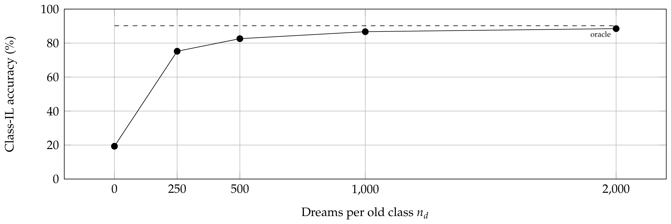
Vanilla local learning collapses to chance, inheriting backpropagation’s forgetting (a direct consequence of Theorem 2). Weight regularization (EWC, SI) does not help in the class-incremental regime, matching the literature [20]. The reason is structural rather than a matter of tuning: a quadratic penalty can protect weights that were important for old classes, but it cannot create the decision boundaries that separate classes never seen together, and in class-incremental learning the model is never shown two tasks’ classes jointly, so no anchor can teach their relative calibration. Replay sidesteps this exactly because it re-presents past classes alongside the new ones. Generative dreaming recovers of the joint ceiling (Figure 12); in the easier task-incremental scenario, where cross-task calibration is not required, the same model reaches . Figure 13 and Figure 14 trace this over the task sequence, vanilla learning ends able to classify only the most recent task, while dreaming retains them all. The number of dreams trades memory for retention ( for ); sampling latent codes from a Gaussian mixture with closes the gap to , points from the oracle (Figure 10).
Figure 10.
Ablation of the dream budget on Split-MNIST. Even a small number of self-generated samples recovers most of the accuracy; returns diminish as approaches the oracle (perfect-memory) bound.
Figure 10.
Ablation of the dream budget on Split-MNIST. Even a small number of self-generated samples recovers most of the accuracy; returns diminish as approaches the oracle (perfect-memory) bound.
A second ablation isolates the cost of the inference itself: how many relaxation steps T the local rule needs to assign credit well. We trained the single-task MNIST classifier () for a fixed number of epochs while varying T, measuring test accuracy and wall-clock time (Figure 11). The result is informative and, at first sight, counter-intuitive: accuracy is essentially flat, at and at (the absolute level sits below the reported above because the per-run training budget is held deliberately small to isolate the effect of T), while wall-clock time grows almost linearly in T (from to s, a increase). For a shallow network a single relaxation step already captures most of the credit-assignment signal, so the extra equilibration is nearly wasted compute. This sharpens the efficiency discussion of Section 7: the per-step locality of the rule is what matters, and one should spend relaxation steps only where they pay off, primarily in deeper networks, where the error must propagate through more layers before the activities settle (the depth barrier discussed in Section 7). It also makes the measured slowdown over backpropagation a worst-case figure tied to large T, not an intrinsic property of local learning.
Figure 11.
Ablation of the number of relaxation steps T in the local classifier (single-task MNIST). Accuracy (left axis, solid) is flat across T; wall-clock time (right axis, dashed) grows roughly linearly. One step already suffices for a shallow network.
Figure 11.
Ablation of the number of relaxation steps T in the local classifier (single-task MNIST). Accuracy (left axis, solid) is flat across T; wall-clock time (right axis, dashed) grows roughly linearly. One step already suffices for a shallow network.
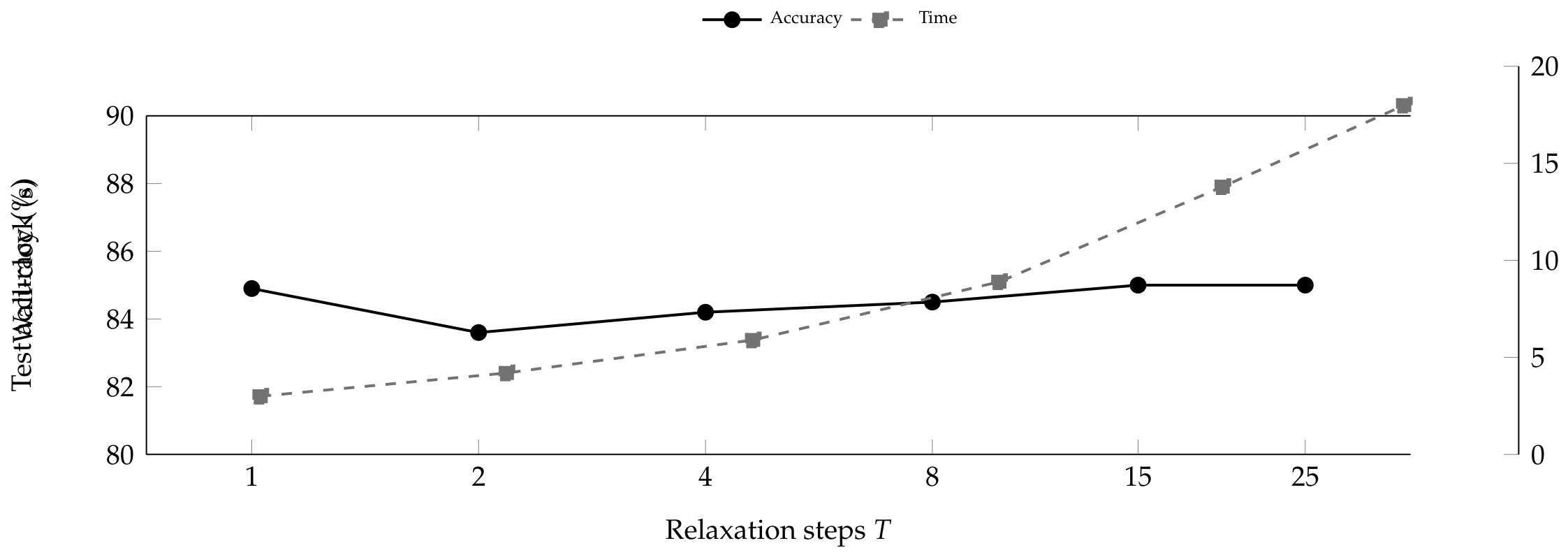
Figure 12.
Class-incremental Split-MNIST. Backpropagation-based regularization (EWC, SI) does not exceed the vanilla/chance level, whereas local generative dreaming reaches , close to the oracle (perfect-memory replay) and the joint-training ceiling.
Figure 12.
Class-incremental Split-MNIST. Backpropagation-based regularization (EWC, SI) does not exceed the vanilla/chance level, whereas local generative dreaming reaches , close to the oracle (perfect-memory replay) and the joint-training ceiling.
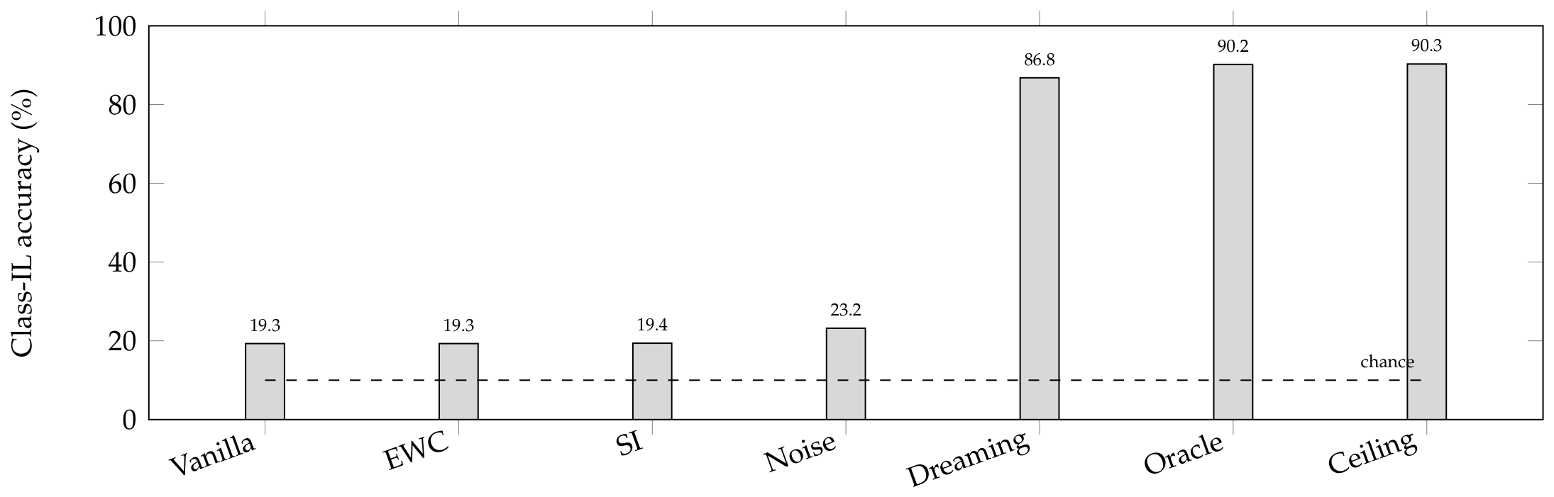
Figure 13.
Forgetting over the task sequence on Split-MNIST (average class-IL accuracy over all tasks seen so far). Vanilla local learning degrades toward chance as new tasks arrive, its accuracy on the first task collapses from to after a single new task, whereas local generative dreaming retains earlier tasks throughout (first-task accuracy stays ).
Figure 13.
Forgetting over the task sequence on Split-MNIST (average class-IL accuracy over all tasks seen so far). Vanilla local learning degrades toward chance as new tasks arrive, its accuracy on the first task collapses from to after a single new task, whereas local generative dreaming retains earlier tasks throughout (first-task accuracy stays ).
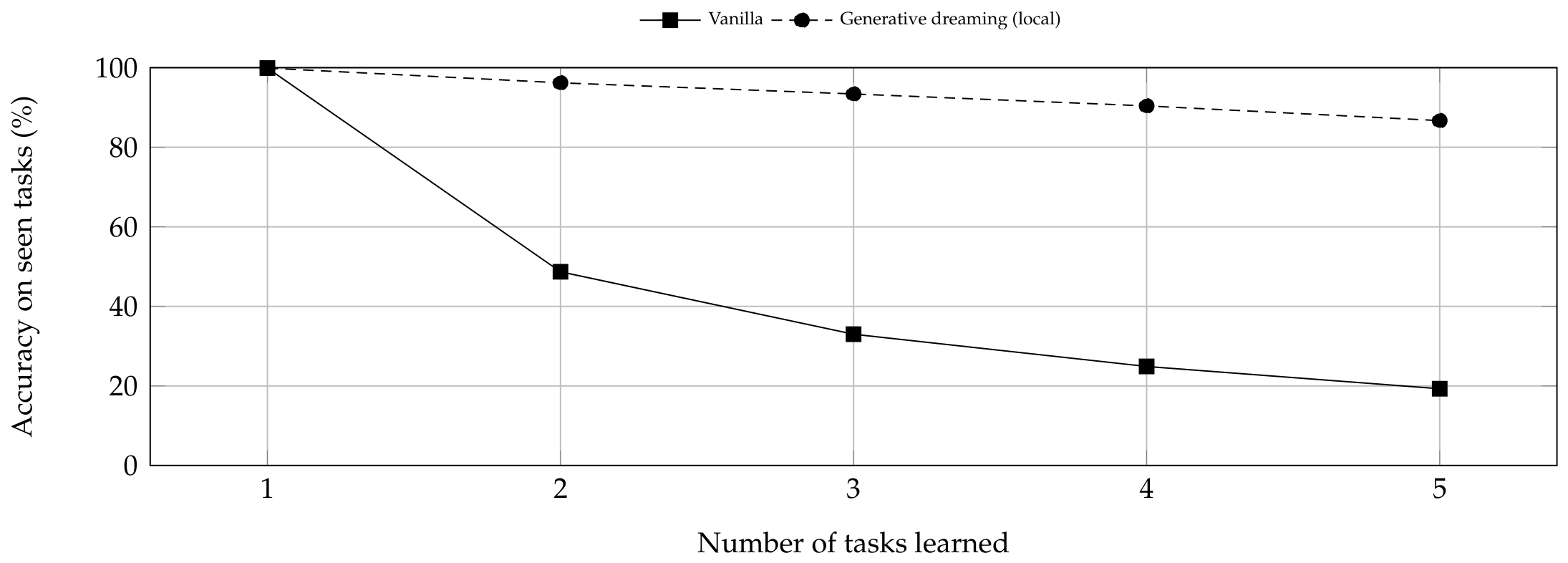
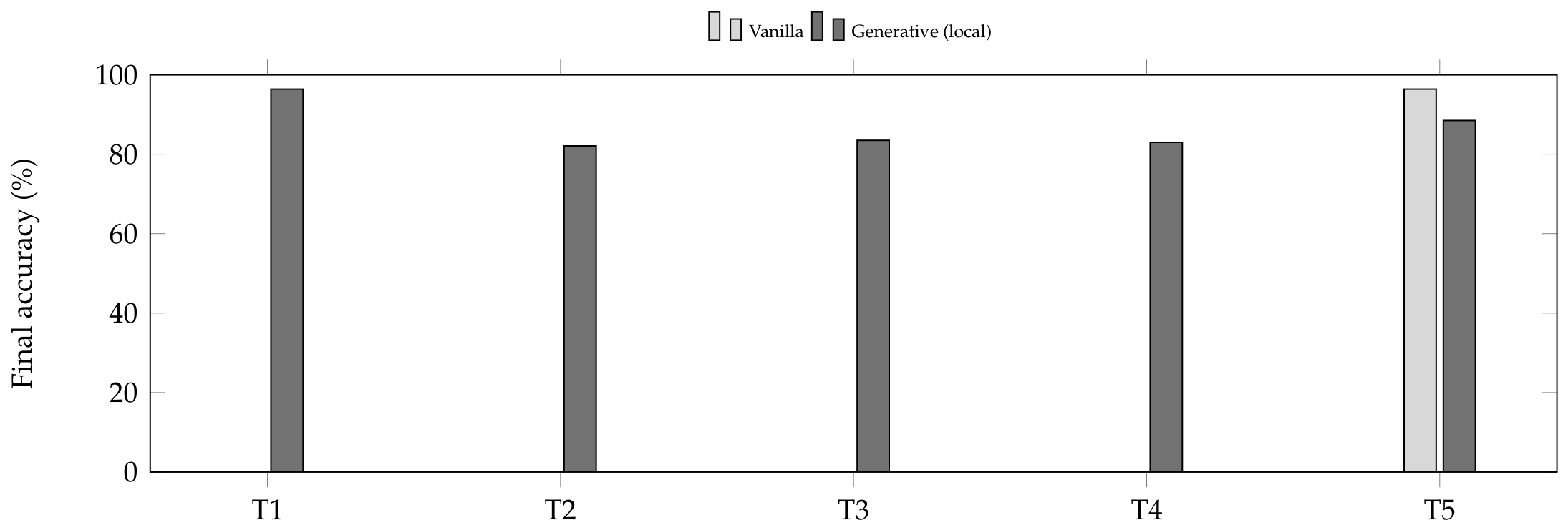
Figure 14.
Per-task accuracy after the full five-task sequence. Vanilla local learning retains only the most recent task (T5) and scores zero on all earlier ones; local generative dreaming retains every task. This is the same phenomenon as Figure 13, viewed as the final distribution over tasks.
Figure 14.
Per-task accuracy after the full five-task sequence. Vanilla local learning retains only the most recent task (T5) and scores zero on all earlier ones; local generative dreaming retains every task. This is the same phenomenon as Figure 13, viewed as the final distribution over tasks.
6.3. Why Dreaming Works: The Data Manifold
Why does self-generated replay help where labelling random noise does not? The answer is geometric. Real data occupy a thin manifold within a high-dimensional ambient space; a useful rehearsal sample must lie on that manifold, because the old classifier was only ever shaped there. We make this precise with a controlled toy in which a 2-D two-moons manifold is embedded in . We measure, for each rehearsal strategy, the residual distance of its samples to the data manifold (the norm of the component orthogonal to the principal subspace). Gaussian noise sits far off the manifold (distance , versus for real data) and barely mitigates forgetting (); a local manifold generator obtained from Oja’s principal-subspace rule [29] places its samples essentially on the manifold (distance ) and all but eliminates forgetting ().
This explains why naive pseudo-rehearsal fails in high dimension [24]: as dimensionality grows, random inputs are almost surely off-manifold, so the old model labels meaningless points and the rehearsal is uninformative. It also identifies why an energy-based network is structurally suited to continual learning: because it is generative, it can dream on its own learned manifold—internal, context-modulated generation in the spirit of brain-inspired replay [25]—whereas a purely discriminative perceptron has no such generator. This geometric account also predicts the dataset-dependence we observe in Section 6: the harder the manifold is to model, the more the quality of the generator (not the continual mechanism) bounds the result.
We confirm this dependence directly by varying the capacity of the generator. Using a stable linear generator, the per-class principal subspace, the fixed point of Oja’s rule [29], we sweep the subspace dimension k and measure class-incremental retention (Figure 15). Retention rises monotonically with k, from with a single principal component to at , and saturates as it approaches the oracle bound; at it already reaches , matching the nonlinear generator’s headline . Two readings follow. First, the continual mechanism is not the bottleneck: even a one-dimensional generator recovers four-fifths of the ceiling, far above the of vanilla learning. Second, the residual gap to the oracle is governed by how faithfully the generator covers the class manifold, exactly the quantity k controls, so a better generator, not a better replay schedule, is the lever for closing it.
Comparative performance
A fair reading of the evidence avoids the overclaim that local learning beats backpropagation outright. Table 11 summarises the honest picture: LEL matches backpropagation in raw accuracy (Theorem 2); it surpasses backpropagation-based regularization (EWC, SI) by a wide margin in class-incremental continual learning when equipped with local generative replay ( vs. ); it lags on current von Neumann hardware in speed and compute; and it holds structural advantages (activation memory, locality, biological plausibility) whose energy payoff is, so far, a hardware projection.
Cross-dataset generality.
Table 12 extends the comparison to Fashion-MNIST and CIFAR-10.
The mechanism generalises across all three datasets. The CIFAR-10 result () is deliberately modest: the joint-training ceiling is only and the oracle reaches , so local dreaming recovers the attainable ceiling. The low ceiling reflects the shallow raw-pixel classifier, not the continual mechanism; the bottleneck is base representation quality (Figure 16).
6.4. Open Problem: Depth and Error Imbalance
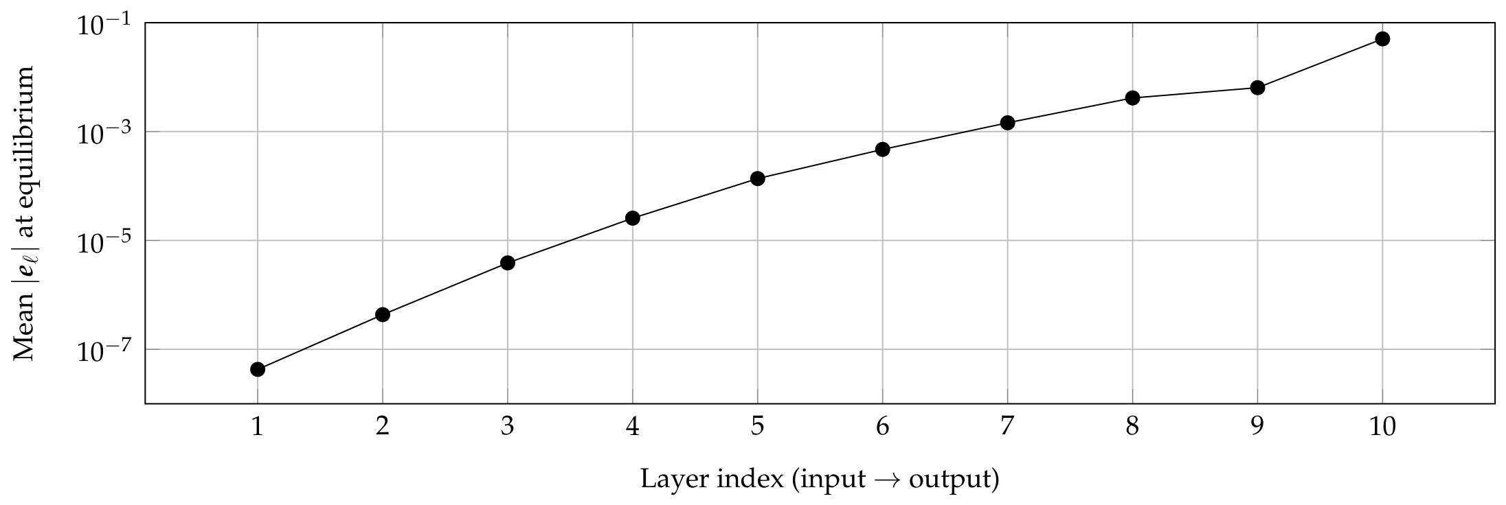
Training a deep LEL network from scratch exhibits a clear depth barrier: at the per-layer equilibrium errors span six orders of magnitude (input-side , output-side ), so deep layers receive almost no learning signal. Growing the network by “grafting” layers incrementally (each healed by local relaxation) improves a depth-8 ten-way network from to , but it does not balance the errors; it works because each layer learns useful features while still near the output. This is essentially greedy layer-wise growth [32], reported here as a characterisation of the open problem, not a solution.
Figure 17.
The depth/error-imbalance barrier in a LEL network: equilibrium prediction errors decay roughly one order of magnitude per layer toward the input, spanning six orders of magnitude, so the deepest layers receive almost no learning signal.
Figure 17.
The depth/error-imbalance barrier in a LEL network: equilibrium prediction errors decay roughly one order of magnitude per layer toward the input, spanning six orders of magnitude, so the deepest layers receive almost no learning signal.
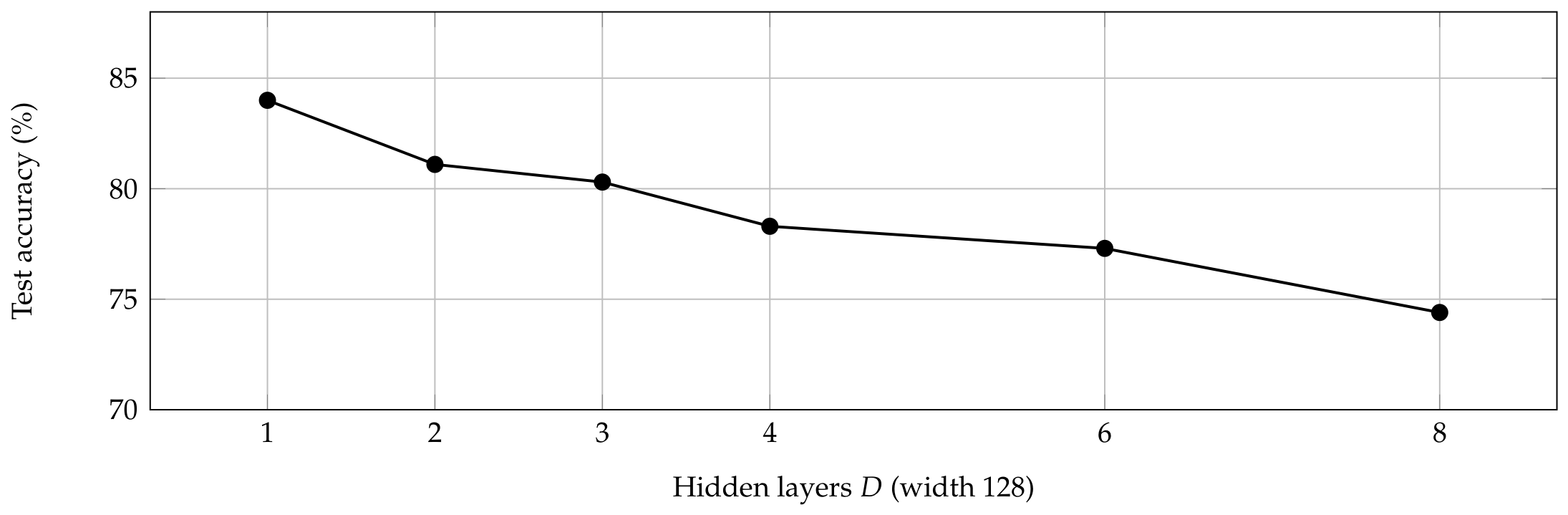
The downstream effect on accuracy is direct. Training a single-task MNIST classifier from scratch at increasing depth (one hidden layer up to eight, all of width 128), test accuracy falls monotonically from to (Figure 18 and Table 13): every layer added near the input is a layer that learns little, so it costs rather than adds capacity. Figure 17 shows the cause (vanishing equilibrium error) and Figure 18 the consequence (lost accuracy); together they bound the problem the remedies of Section 7 must solve before local learning can match backpropagation on deep networks.
Figure 18.
Effect of depth on a single-task MNIST classifier trained from scratch with the local rule. Accuracy declines monotonically as depth grows, because the layers near the input receive a vanishing equilibrium error (Figure 17) and therefore barely learn.
Figure 18.
Effect of depth on a single-task MNIST classifier trained from scratch with the local rule. Accuracy declines monotonically as depth grows, because the layers near the input receive a vanishing equilibrium error (Figure 17) and therefore barely learn.
7. Hardware, Applications, and Open Challenges
The structural properties of energy-based local learning—locality, generativity and in-memory compatibility—motivate dedicated hardware research and deployment contexts that the preceding benchmark cannot reach.
7.1. Hardware and Neuromorphic Realisations
A central motivation for backpropagation-free learning is hardware. On conventional von Neumann machines the dominant energy cost of both training and inference is not arithmetic but data movement: fetching weights and activations between memory and compute units costs one to three orders of magnitude more energy than the multiply–accumulate that consumes them [4]. Backpropagation aggravates this in two ways: it must store the entire forward activation graph for the backward pass, and it requires a transposed copy of the forward weights to route the error, the weight-transport problem [16], which has no natural physical realisation. Local methods avoid both: the error and presynaptic activity needed to update a synapse are available in situ, so the update can, in principle, happen where the weight is stored.
In-memory and analog computing.
This locality is precisely what in-memory and analog accelerators exploit. In a memristor or resistive crossbar, the synaptic weight is the conductance of a device, so a matrix–vector product is performed in place by Ohm’s and Kirchhoff’s laws, computation and memory are co-located and weight movement is eliminated [42]. The for deep learning this means lower data-transfer cost, higher compute efficiency per joule, and training and inference on the same device [43]. The feasibility of training in such memory is no longer hypothetical: analogue non-volatile memory has trained networks to software-equivalent accuracy on MNIST and CIFAR by performing the multiply–accumulate in place at the location of the weights [63], exactly the regime in which a local update rule that needs no transported weights is most at home (Figure 19).
In-situ local training on crossbars.
The point that matters for this survey is that crossbars favour local learning rules. Self-adaptive in-situ learning has been demonstrated in multilayer memristor networks [44]; parallel in-situ training has been realised with electrochemical RAM [34]; and activity-difference training, updating weights from the difference between two network states, a contrastive/equilibrium-style local rule that avoids an explicit backward pass, has been run directly on memristor crossbars [45]. These results make energy-based, local credit assignment a natural algorithmic match for analog hardware. The principal obstacles are device-level: non-linear and stochastic conductance updates and device-to-device variability degrade training accuracy, and overcoming them is an active hardware–algorithm co-design problem [46].
Neuromorphic processors and on-chip learning.
Digital neuromorphic processors provide event-driven, massively parallel substrates with on-chip plasticity: IBM TrueNorth runs one million spiking neurons below 100 mW [76]; Intel Loihi pioneered on-chip local learning [47]; its successor Loihi 2 and SpiNNaker2 are current event-driven platforms in which states and weights are held in local memory beside the compute [76,77]. Local rules are a natural fit, and EqSpike is the clearest algorithmic example: it recasts equilibrium propagation in a spike-driven form and, when mapped to silicon, is projected to cut inference energy by about three orders of magnitude and training by about two relative to a GPU, while supporting online on-chip learning [12]. A caveat: on-chip learning can itself dominate the energy budget, so the update rule must be hardware-aware [46].
Spiking implementations.
Bridging continuous local-learning theory and spiking hardware is an active area. Surrogate-gradient methods make spiking networks trainable by smoothing the non-differentiable spike [33], and analog surrogate-gradient training has been demonstrated on neuromorphic substrates [34]. The conversion of rate-based relaxation into event-driven dynamics, and the device variability such mappings must tolerate, remain the central trade-offs [46].
7.2. Representative Application Contexts
The benchmark focused on continual learning, but local equilibrium networks are also relevant where on-device adaptation, limited memory, or biological plausibility constrain the design.
Continual and lifelong learning.
This is the application tested here. Sequential learners must update after deployment without retaining every past example, and energy-based local networks offer a natural storage-free replay mechanism because they can generate samples from their own learned structure [20,67,68]. The benchmark in Section 6 should be read as a minimal reproducible case of that idea, not as a final solution for all lifelong-learning settings.
Perception and representation learning.
Predictive coding began as a model of cortical perception and remains useful as a generative representation learner: a hierarchy that minimises prediction error can also learn features and reconstruct missing or corrupted inputs [7,8,69,73]. For the present paper, this matters because replay quality depends on whether the generator captures the data manifold; the CIFAR-10 limitation is therefore partly a representation limitation.
Edge, robotics and neuromorphic deployment.
Local updates are attractive when devices face strict memory, bandwidth and energy budgets, as in embedded perception, adaptive robotics and streaming sensorimotor control [12,34,47,76,77]. The claim is conditional: on ordinary CPUs the iterative relaxation is slower than backpropagation, but on in-memory or neuromorphic substrates locality may reduce data movement. That hardware advantage remains to be measured for the full continual pipeline.
7.3. Open Challenges and Research Programme
The evidence assembled in this survey—coherent theory, a reproducible case study and a hardware case that is strong in principle—also marks where the field needs to go next. Three barriers must be overcome before local continual learning can move beyond image benchmarks, and the community is actively working on all three.
Depth and scaling.
The depth/error-imbalance barrier is the central open problem of local learning. Backpropagation itself only conquered very deep networks through residual connections [5] and normalisation [6]; local learning still lacks a comparably mature toolkit, and importing these ideas is part of the active effort below. As our testbed shows (Section 6, Figure 17), training a deep energy-based network from scratch leaves the layers near the input with vanishingly small equilibrium errors, so they barely learn; vanilla predictive coding is known to degrade once the stack grows beyond a handful of layers. Several complementary remedies are under active investigation, which we group by the mechanism they target.
Parameterisation, re-balancing and better schedules.
Depth-aware parameterisation, adapting P-style scaling to inference dynamics, keeps activity learning rates stable across width and depth. Precision-weighting of per-layer errors redistributes the energy during relaxation, the natural remedy for the imbalance our testbed exhibits (Figure 17). Prospective-configuration-style training separates inference from plasticity, making the learning rule easier to analyse and improving sample efficiency [10,31].
EqProp at scale and shared benchmarks.
Reducing the bias of the finite-nudge gradient estimator enabled scaling to deep convolutional networks [36]; standardised benchmarks are beginning to make cross-method comparison fair [31]. The problem is actively contested but not closed, and our reproducible testbed (Figure 17) is a small, transparent instrument for studying it.
Nudge, weight symmetry and the two-phase requirement.
Energy-based methods classically require either an infinitesimal nudge (EqProp) or clamped outputs (PC), and often symmetric weights, requirements that are awkward biologically and on hardware. Recent work relaxes the infinitesimal-nudge assumption with finite-nudge formulations, while feedback-alignment results show that exact weight symmetry is not strictly necessary for useful learning [16]. Reducing or eliminating the two-phase structure, and quantifying the bias introduced by finite nudges, remain open.
Modern architectures.
Almost all local-learning results concern multilayer perceptrons and convolutional networks; extending local credit assignment to the architectures that dominate contemporary AI, attention and transformers [3], is largely unexplored. Sequential tasks remain dominated by LSTM networks and their variants [2]; a local formulation of attention-based sequence processing has not yet demonstrated comparable accuracy on standard benchmarks. Whether an energy-based or forward-only formulation of self-attention can match backpropagation is, to our knowledge, an open and high-value question.
Theory and evaluation.
Theoretical understanding is advancing (Lyapunov stability of the inference dynamics [60], the infinitesimal-inference limit that links these methods to backpropagation [9,11]), but generalisation guarantees, convergence rates under realistic conditions, and the interaction between inference accuracy and learning remain partially open. On the empirical side, the field has historically suffered from inconsistent benchmarks; unified evaluation suites and reproducible studies such as this one are needed for cumulative progress [31].
Computational and energy trade-offs.
On von Neumann hardware LEL is more expensive: the T-step relaxation costs the operations of backpropagation and was slower in our CPU measurement; we claim no speed advantage there. Its structural benefits are (i) activation memory vs. , and (ii) locality, which permits execution on in-memory and neuromorphic substrates that backpropagation cannot easily use because of the weight-transport problem [16].
The structural reason is data movement: off-chip DRAM access costs about two orders of magnitude more energy than the arithmetic it feeds [4], so on von Neumann hardware training energy is dominated by shuttling weights and activations rather than by multiply–accumulate operations. Because every LEL update reads only quantities already present at the synapse, it can execute where the weight is stored, eliminating the dominant data-movement term and projecting a 120– reduction relative to backpropagation on DRAM—consistent with figures reported for spike-driven equilibrium and surrogate-gradient learning on neuromorphic substrates [12,33,34]. Backpropagation cannot occupy this regime at all because its backward pass requires a transported copy of the weights. We stress that this is a projection from per-operation figures, not a device measurement; the numbers in Table 14 quantify the on-hardware cost.
Empirical failures and scope limits
The negative results are first-class findings, not caveats appended after the fact. They separate what failed empirically from what remains outside the scope of this benchmark.
Negative empirical results
Vanilla local learning does not beat backpropagation in accuracy or forgetting; because the equilibrium update approaches the backpropagation gradient (Theorem 2), it inherits catastrophic forgetting unless an additional retention mechanism is added. Weight regularization also failed in the class-incremental setting: EWC and SI stayed near chance, and the energy-based EWC variant destabilised relaxation by pulling weights away from the contractive regime required by Proposition 1. Noise replay failed for a different reason: random samples lie off the data manifold and therefore do not recreate meaningful old-task decision boundaries. Finally, simple “free” fixes for depth, including metaplastic per-synapse learning rates and homeostatic norm control, did not remove the error-imbalance barrier.
Depth limitation
The strongest algorithmic limitation is depth. In the current implementation, layers near the input receive equilibrium errors several orders of magnitude smaller than layers near the output, so adding depth can reduce rather than improve accuracy (Figure 17 and Table 13). Grafting helps by allowing early layers to learn while they are still close to the output, but it does not solve the underlying imbalance. The manuscript therefore does not claim that LEL is ready for very deep networks; it identifies a reproducible failure mode that future local-learning methods must overcome.
Computational-cost limitation.
LEL is not faster on standard von Neumann hardware. The iterative relaxation requires multiple state updates per training sample, making it roughly 5– more expensive in our measurements than a matched backpropagation baseline (Table 14). The possible advantage is structural rather than immediate: local updates reduce activation storage and may avoid costly data movement when executed in memory or on neuromorphic hardware. Until that full pipeline is implemented and measured on a device, the energy argument remains a projection.
CIFAR-10 limitation
The CIFAR-10 result is deliberately modest. A final accuracy of would be unacceptable if the paper were claiming competitiveness with modern backpropagation-trained CNNs or Transformers. That is not the claim. The experiment tests whether the same local replay mechanism still recovers most of the available ceiling when the base model is a shallow raw-pixel classifier. It does ( out of a ceiling), but the low ceiling shows that useful deployment will require stronger local representations, feature-space replay or a more capable local generator.
Scope limitation
The benchmark uses small networks, public image datasets and controlled task sequences. It does not address large-scale foundation models, naturalistic non-stationarity, continual reinforcement learning or measured hardware energy. These omissions are intentional: the purpose is to provide a clean reference point where the role of local credit assignment, replay, generator quality and memory budget can be inspected without hidden pretrained components.
Research programme
Table 15 translates the open challenges above into testable tasks, tracing a path from the current proof of concept—local generative replay on image benchmarks—toward scalable, hardware-native continual learning without backpropagation.
8. Conclusions
This survey set out to answer one concrete question: can a backpropagation-free network keep learning without forgetting? The answer is yes, but only with the right retention mechanism, and that finding requires common, reproducible ground rather than the scattered formulations, notations and benchmarks that have fragmented the local-learning literature. We organised the two halves of the problem (backpropagation-free credit assignment and continual learning) into one taxonomy, expressed the energy-based family through a single transparent formulation, re-derived and numerically re-validated its core theory, and ran a controlled empirical case study across three datasets and two independent implementations. The intent was never a new learning rule, but a synthesis, reproducibility package and benchmark that make the field legible and give others a concrete baseline to extend or falsify.
Empirical synthesis
Across three datasets and two independent implementations the results converge on a clear hierarchy: generative dreaming is the only retention mechanism that works reliably under the strict Class-IL protocol. EWC and SI remain near chance; noise replay fails because random samples lie off the data manifold; only locally generated “dream” samples, drawn from the energy-based model’s own learned distribution, recreate the decision boundaries needed to prevent catastrophic forgetting. The effect is quantitatively large and general: local dreaming reaches 86– retention on Split-MNIST ( of the joint-training ceiling) and 96– of the ceiling on Fashion-MNIST and CIFAR-10, reproduced in a second independent implementation. The remaining gap to the oracle ceiling is governed by generator quality, not by the continual mechanism—a conclusion the generator-capacity ablation confirms directly (Figure 15).
What the evidence shows
Four findings hold up across every dataset and both implementations. First, local energy-based learning matches backpropagation in supervised accuracy. This is well understood by now, because the local update equals the backpropagation gradient in the small-nudge limit (Theorem 2, Figure 8), and that we confirm rather than claim as novel. Second, precisely because of this equivalence, vanilla local learning inherits catastrophic forgetting; locality is not, by itself, a cure. Third, the cure is structural rather than regularisational: weight anchoring (EWC, SI) fails in the class-incremental regime, and when ported to the energy-based setting it even destabilises the inference relaxation. Generative replay, by contrast, succeeds, and energy-based networks support it natively because the same network that discriminates can dream on its own learned data manifold. Fourth, the resulting effect is large and general: local dreaming converts chance-level forgetting into 86– retention on Split-MNIST ( of the joint-training ceiling) and reaches 96– of the ceiling on Fashion-MNIST and CIFAR-10, reproduced in a second programming language. The limit is as clear as the result: the absolute number is set by the quality of the base classifier and the generator, not by the continual mechanism, and we isolated this experimentally rather than just asserted it, showing retention rise monotonically with generator capacity toward the oracle (Figure 15).
Why it matters
These results recast backpropagation as one credit-assignment choice among several rather than a law of learning. The case for the alternatives is not, today, that they are more accurate; they are not, a conclusion consistent with broader reviews of continual and biologically inspired learning [19,65,66]. It is that they are structurally different in ways that matter for where computing is heading: they are local, so they need neither a stored computation graph nor a transported copy of the weights; they are generative, so they can rehearse the past without storing it; and they update online, which is the native regime of systems that must keep learning after deployment. These are exactly the properties an energy-, memory- and data-movement-constrained future rewards, and they are the reason the intersection of local learning and continual learning, the niche this survey occupies, is worth taking seriously.
What remains open
We have been deliberate about not overclaiming. On conventional von Neumann hardware the approach is several times slower and more energy-hungry than backpropagation; its energy advantage is a principled projection onto in-memory and neuromorphic substrates, not a measurement we made. Training degrades in very deep networks because the layerwise equilibrium errors become exponentially imbalanced. We reproduce this open problem honestly, and the community is actively attacking it through reparameterisation, energy re-balancing and better inference schedules (Section 7). And the extension of local credit assignment to the architectures that dominate contemporary AI, namely attention and transformers, remains almost entirely unexplored. We also reported, as carefully as the positive results, what did not work: naive energy sampling diverges, regularisation destabilises the relaxation, and the most natural “free” fixes for the depth barrier did not help. These negative results are part of the contribution, because they delimit the design space for those who follow.
Outlook
The most important next step is to stop projecting and start measuring: to express the relaxation and the generative dreaming in a spiking or analog form and report joules on real neuromorphic devices, converting the structural energy argument into evidence. In parallel, importing the depth remedies surveyed here into the continual-learning pipeline, and probing whether an energy-based or forward-only formulation of self-attention can match backpropagation, would tell us whether local learning scales to the problems that matter most. We have tried to lower the barrier to all of this by releasing the unified formulation and every experiment as small, dependency-light, independently reproduced scripts. The primary contribution of this review is to establish a reproducible baseline and clarify the research agenda for local credit assignment in continual learning—not to resolve it.
Author Contributions
Conceptualization, methodology, software, validation, writing—original draft preparation, writing—review and editing: C.H.V.N. The author has read and agreed to the published version of the manuscript.
Funding
This research received no external funding.
Data Availability Statement
All code and scripts used in this benchmark are publicly available at https://github.com/chvn00/LEL.
Conflicts of Interest
The author declares no conflict of interest.
Appendix A. Terminology
Table A1 fixes how terms are used in this paper. They are included because the same words are sometimes used differently across the backpropagation-free and continual-learning literatures.

Table A1.
Terminology used throughout the paper.
| Term | Meaning in this paper |
|---|---|
| Backpropagation-free | The credit-assignment update does not require a global backward pass through the computational graph. The term does not imply better accuracy, lower cost on CPUs/GPUs, or continual learning by itself. |
| Local update | A synaptic update uses quantities available at the connected units, typically pre-synaptic activity and post-synaptic prediction error or state. |
| Energy-based learning | Inference is cast as relaxation of neural states to reduce an energy or free-energy objective; learning updates parameters using the equilibrium states. |
| LEL | The particular local equilibrium formulation used in this paper: a transparent predictive-coding-style network with squared prediction errors and local Hebbian updates. |
| Dreaming | Storage-free generative replay: pseudo-samples of old classes are generated by a local generator and mixed with current-task data. |
| Oracle replay | Replay using stored real examples from past tasks. It is a bound, not a storage-free method. |
| Class-incremental learning | The model must classify among all classes seen so far without being told the task identity at test time. |
| Task-incremental learning | The model is told the task identity or evaluated within the correct task head at test time. |
| Generator bottleneck | The situation in which replay would work with perfect samples, but the learned generator does not cover the old data manifold well enough. |
| Depth/error imbalance | The decay of equilibrium errors across layers in deep local networks, which leaves early layers with too little learning signal. |
Appendix B. Implementation Notes for LEL
Appendix B records several implementation details that are easy to miss when translating the equations into code. They are not new theory, but they are important for reproducing the behaviour reported in the paper.
Appendix B.1. Signs and Objectives
In the supervised, fully clamped version used for most experiments, the output state is fixed to the target during relaxation. The layer error is , and the local weight increment is proportional to . This sign is chosen so that the update descends the reduced free energy. It is tempting to compare this update directly with the backpropagation gradient of the supervised loss, but in the fully clamped regime the objectives are not identical. The exact comparison to backpropagation is the nudged regime of Theorem 2, where the output is softly pulled toward the target and the limit is taken. This distinction explains why the theorem-validation script reports two different behaviours: full clamping saturates below perfect cosine alignment, while the small-nudge update approaches alignment one.
Appendix B.2. Relaxation Stability
The inference step size is a stability parameter as much as a speed one. If is too small, the network may not approach equilibrium within the chosen budget T; if it is too large, the activities oscillate or diverge. A simple diagnostic is to track the free energy or the norm of the state gradient across relaxation steps. In a stable run, the energy should decrease or at least settle after a small transient caused by finite-step discretisation. When the energy grows systematically, increasing epochs or replay samples will not fix the experiment; the state dynamics themselves are outside the contractive regime assumed by Proposition 1.
Appendix B.3. Finite Inference and Biased Updates
The envelope theorem gives the local gradient at equilibrium. In code, equilibrium is approximated by a finite number of steps. The resulting update is biased, and the bias is controlled by both the relaxation budget T and the conditioning of the energy landscape. This is why T should be reported even when accuracy appears insensitive to it. A shallow network may work with or because the forward initialisation is already close to equilibrium; a deeper network may require more steps, different precisions or residual dynamics before the same claim is meaningful.
Appendix B.4. Clamping, Nudging and Test-Time Inference
Training and testing use different operations. During training, the input and either the output target (clamped case) or a soft output penalty (nudged case) participate in the energy. During testing, the experiments here use the feedforward prediction for classification, because no target is available. One can also run free relaxation at test time, but then the protocol must specify which variables are clamped, which are free, and how the predicted label is read out. Mixing these conventions across methods can change the result, especially in recurrent or strongly energy-based models.
Appendix B.5. Generator Training and Labelling
The dreaming pipeline contains two models: a generator for samples and a frozen classifier for labels. The generator should be trained only on the current class data when that class is first seen. Later, it is sampled without access to old raw data. The labels assigned to dreams come from the frozen previous classifier in the general pseudo-rehearsal setting; in controlled variants one may use class labels directly, but then the experiment is no longer testing the same self-labelling mechanism. This difference should be stated because it affects whether errors in the old classifier are propagated into the rehearsal set.
Appendix B.6. Minimal Pseudocode for One Task Transition
The following task-transition view is often easier to implement than the full algorithmic listing. Let be the classifier after task , and let be the stored local generators for old classes. For a new task with data , create a training set
Then train the classifier locally on , train new generators for the new classes, and freeze a copy of the classifier for the next labelling step. The important feature is that past raw data never enter ; only generated samples do.
Abbreviations
Abbreviations used in this manuscript:
| LEL | Local Equilibrium Learning |
| BP | Backpropagation |
| PC | Predictive Coding |
| EqProp | Equilibrium Propagation |
| FA | Feedback Alignment |
| TP | Target Propagation |
| EWC | Elastic Weight Consolidation |
| SI | Synaptic Intelligence |
| CL | Continual Learning |
| Class-IL | Class-Incremental Learning |
| Task-IL | Task-Incremental Learning |
| BIR | Brain-Inspired Replay |
| MLP | Multilayer Perceptron |
| STDP | Spike-Timing-Dependent Plasticity |
| GPU | Graphics Processing Unit |
References
- Baydin, A.G.; Pearlmutter, B.A.; Radul, A.A.; Siskind, J.M. Automatic differentiation in machine learning: a survey. J. Mach. Learn. Res. 2018, 18, 1–43. [Google Scholar]
- Sherstinsky, A. Fundamentals of recurrent neural network (RNN) and long short-term memory (LSTM) network. Phys. D. 2020, 404, 132306. [Google Scholar] [CrossRef]
- Vaswani, A.; et al. Attention is all you need. NeurIPS 2017. [Google Scholar] [CrossRef]
- Sze, V.; Chen, Y.-H.; Yang, T.-J.; Emer, J.S. Efficient processing of deep neural networks: a tutorial and survey. Proc. IEEE 2017, 105(12), 2295–2329. [Google Scholar] [CrossRef]
- He, K.; Zhang, X.; Ren, S.; Sun, J. Deep residual learning for image recognition. CVPR, 2016. [Google Scholar]
- Santurkar, S.; Tsipras, D.; Ilyas, A.; Madry, A. How does batch normalization help optimization? Proc. NeurIPS 2018, 31, 2483–2493. [Google Scholar]
- Millidge, B.; Tschantz, A.; Buckley, C.L. Predictive coding approximates backprop along arbitrary computation graphs. Neural Comput. 2022, 34(6), 1280–1317. [Google Scholar] [CrossRef]
- Bogacz, R. A tutorial on the free-energy framework for modelling perception and learning. J. Math. Psychol. 2017, 76, 198–211. [Google Scholar] [CrossRef] [PubMed]
- Whittington, J.C.R.; Bogacz, R. An approximation of the error backpropagation algorithm in a predictive coding network with local Hebbian synaptic plasticity. Neural Comput. 2017, 29, 1229–1262. [Google Scholar] [CrossRef] [PubMed]
- Song, Y.; Millidge, B.; Salvatori, T.; Lukasiewicz, T.; Xu, Z.; Bogacz, R. Inferring neural activity before plasticity as a foundation for learning beyond backpropagation. Nat. Neurosci. 2024. [Google Scholar] [CrossRef] [PubMed]
- Scellier, B.; Bengio, Y. Equilibrium propagation: bridging the gap between energy-based models and backpropagation. Front. Comput. Neurosci. 2017, 11, 24. [Google Scholar] [CrossRef] [PubMed]
- Martin, E.; et al. EqSpike: spike-driven equilibrium propagation for neuromorphic implementations. iScience 2021, 24, 102222. [Google Scholar] [CrossRef] [PubMed]
- Kohan, A.; Rietman, E.A.; Siegelmann, H.T. Signal propagation: a framework for learning in a forward pass. IEEE TNNLS, 2023. [Google Scholar]
- Closed-form feedback-free learning with forward projection. Nat. Commun. 2026. [CrossRef] [PubMed]
- Nøkland, A.; Eidnes, L.H. Training neural networks with local error signals. ICML, 2019. [Google Scholar]
- Lillicrap, T.P.; Cownden, D.; Tweed, D.B.; Akerman, C.J. Random synaptic feedback weights support error backpropagation for deep learning. Nat. Commun. 2016, 7, 13276. [Google Scholar] [CrossRef] [PubMed]
- Nøkland, A. Direct feedback alignment provides learning in deep neural networks. NeurIPS, 2016. [Google Scholar]
- Meulemans, A.; Carzaniga, F.S.; Suykens, J.A.K.; Sacramento, J.; Grewe, B.F. A theoretical framework for target propagation. Proc. NeurIPS 2020, 33, 20024–20036. [Google Scholar]
- De Lange, M.; Aljundi, R.; Masana, M.; Parisot, S.; Jia, X.; Leonardis, A.; Slabaugh, G.; Tuytelaars, T. A continual learning survey: Defying forgetting in classification tasks. In IEEE Trans. Pattern Anal. Mach. Intell.; 2021. [Google Scholar] [CrossRef] [PubMed]
- van de Ven, G.M.; Tuytelaars, T.; Tolias, A.S. Three types of incremental learning. Nat. Mach. Intell. 2022, 4, 1185–1197. [Google Scholar] [CrossRef] [PubMed]
- Kirkpatrick, J.; et al. Overcoming catastrophic forgetting in neural networks. PNAS 2017, 114, 3521–3526. [Google Scholar] [CrossRef] [PubMed]
- Zenke, F.; Poole, B.; Ganguli, S. Continual learning through synaptic intelligence. ICML, 2017. [Google Scholar]
- Aljundi, R.; et al. Memory aware synapses: learning what (not) to forget. ECCV, 2018. [Google Scholar]
- Shin, H.; Lee, J.K.; Kim, J.; Kim, J. Continual learning with deep generative replay. NeurIPS 2017. [Google Scholar] [CrossRef]
- van de Ven, G.M.; Siegelmann, H.T.; Tolias, A.S. Brain-inspired replay for continual learning with artificial neural networks. Nat. Commun. 2020, 11, 4069. [Google Scholar] [CrossRef] [PubMed]
- Rebuffi, S.-A.; Kolesnikov, A.; Sperl, G.; Lampert, C.H. iCaRL: incremental classifier and representation learning. CVPR, 2017. [Google Scholar]
- Masse, N.Y.; Grant, G.D.; Freedman, D.J. Alleviating catastrophic forgetting using context-dependent gating and synaptic stabilization. PNAS 2018, 115, E10467–E10475. [Google Scholar] [CrossRef] [PubMed]
- Continual sequence modeling with predictive coding. In Front. Neurorobot.; 2022.
- Pehlevan, C.; Mohan, S.; Chklovskii, D.B. Blind nonnegative source separation using biological neural networks. Neural Comput. 2017, 29(11), 2925–2954. [Google Scholar] [CrossRef] [PubMed]
- Benna, M.K.; Fusi, S. Computational principles of synaptic memory consolidation. Nat. Neurosci. 2016, 19, 1697–1706. [Google Scholar] [CrossRef] [PubMed]
- Effective methods and framework for energy-based local learning of deep neural networks. Front. Artif. Intell. 2025. [CrossRef] [PubMed]
- Yoon, J.; Yang, E.; Lee, J.; Hwang, S.J. Lifelong learning with dynamically expandable networks. Proc. ICLR, 2018. [Google Scholar]
- Neftci, E.O.; Mostafa, H.; Zenke, F. Surrogate gradient learning in spiking neural networks. IEEE Signal Process. Mag. 2019, 36, 51–63. [Google Scholar] [CrossRef]
- Surrogate gradients for analog neuromorphic computing. PNAS, 2022.
- Xiao, H.; Rasul, K.; Vollgraf, R. Fashion-MNIST: a novel image dataset for benchmarking machine learning algorithms. Zalando Res. Technical Report. 2017. [Google Scholar] [CrossRef]
- Laborieux, A.; Ernoult, M.; Scellier, B.; Bengio, Y.; Grollier, J.; Querlioz, D. Scaling equilibrium propagation to deep ConvNets by drastically reducing its gradient estimator bias. Front. Neurosci. 2021, 15, 633674. [Google Scholar] [CrossRef] [PubMed]
- Generative negative replay for continual learning. Neural Netw. 2023, 162, 369–383. [CrossRef] [PubMed]
- CALM: Continual associative learning model via sparse distributed memory. Technologies 2025, 13, 587. [CrossRef]
- Aslam, M.; et al. Continual learning inspired by brain functionality: a comprehensive survey. Int. J. Intell. Syst. 2025. [Google Scholar] [CrossRef]
- Scodellaro, R.; et al. Training convolutional neural networks with the forward–forward algorithm. Sci. Rep., 2025. [Google Scholar]
- Papachristodoulou, A.; et al. Convolutional channel-wise competitive learning for the forward-forward algorithm. AAAI, 2024. [Google Scholar]
- Bring memristive in-memory computing into general-purpose machine learning: a perspective. APL Mach. Learn. 2023, 1, 040901. [CrossRef]
- Hardware-aware training for large-scale and diverse deep learning inference workloads using in-memory computing-based accelerators. Nat. Commun. 2023, 14, 5282. [CrossRef] [PubMed]
- Efficient and self-adaptive in-situ learning in multilayer memristor neural networks. Nat. Commun. 2018, 9, 2385. [CrossRef] [PubMed]
- Activity-difference training of deep neural networks using memristor crossbars. Nat. Electron. 2022, 6, 45–51. [CrossRef]
- Difficulties and approaches in enabling learning-in-memory using crossbar arrays of memristors. Neuromorph. Comput. Eng. 2024. [CrossRef] [PubMed]
- Davies, M.; et al. Loihi: a neuromorphic manycore processor with on-chip learning. IEEE Micro 2018, 38, 82–99. [Google Scholar] [CrossRef]
- Can neuromorphic computing help reduce AI’s high energy cost? A perspective. (perspective) 2025. [CrossRef]
- Laborieux, A.; Zenke, F. Holomorphic equilibrium propagation computes exact gradients through finite size oscillations. NeurIPS, 2022. [Google Scholar]
- Scellier, B.; et al. Energy-based learning algorithms for analog computing: a comparative study. NeurIPS, 2023. [Google Scholar]
- Salvatori, T.; Pinchetti, L.; Millidge, B.; Song, Y.; et al. Learning on arbitrary graph topologies via predictive coding. NeurIPS, 2022. [Google Scholar]
- Tang, M.; Salvatori, T.; Millidge, B.; Song, Y.; Lukasiewicz, T.; Bogacz, R. Recurrent predictive coding models for associative memory employing covariance learning. PLoS Comput. Biol. 2023. [Google Scholar] [CrossRef] [PubMed]
- Millidge, B.; Salvatori, T.; Song, Y.; Lukasiewicz, T.; Bogacz, R. Predictive coding: towards a future of deep learning beyond backpropagation? IJCAI 2022. [Google Scholar] [CrossRef]
- Hooker, S. The hardware lottery. Commun. ACM 2021, 64, 58–65. [Google Scholar] [CrossRef]
- Lillicrap, T.P.; Santoro, A.; Marris, L.; Akerman, C.J.; Hinton, G. Backpropagation and the brain. Nat. Rev. Neurosci. 2020, 21, 335–346. [Google Scholar] [CrossRef] [PubMed]
- Li, Z.; Hoiem, D. Learning without forgetting. IEEE Trans. Pattern Anal. Mach. Intell. 2018, 40, 2935–2947. [Google Scholar] [CrossRef] [PubMed]
- Lopez-Paz, D.; Ranzato, M. Gradient episodic memory for continual learning. NeurIPS 2017, 6467–6476. [Google Scholar]
- Mallya, A.; Lazebnik, S. PackNet: adding multiple tasks to a single network by iterative pruning. CVPR 2018, 7765–7773. [Google Scholar] [CrossRef]
- Krotov, D.; Hopfield, J.J. Dense associative memory for pattern recognition. NeurIPS 2016, 1172–1180. [Google Scholar]
- Ramsauer, H.; Schäfl, B.; Lehner, J.; Seidl, P.; Widrich, M.; Adler, T.; Gruber, L.; Holzleitner, M.; Pavlović, M.; Sandve, G.K.; et al. Hopfield networks is all you need. ICLR, 2021. [Google Scholar]
- Zenke, F.; Neftci, E.O. Brain-inspired learning on neuromorphic substrates. Proc. IEEE 2021, 109(5), 935–950. [Google Scholar] [CrossRef]
- Roy, K.; Jaiswal, A.; Panda, P. Towards spike-based machine intelligence with neuromorphic computing. Nature 2019, 575, 607–617. [Google Scholar] [CrossRef] [PubMed]
- Ambrogio, S.; Narayanan, P.; Tsai, H.; Shelby, R.M.; Boybat, I.; di Nolfo, C.; et al. Equivalent-accuracy accelerated neural-network training using analogue memory. Nature 2018, 558, 60–67. [Google Scholar] [CrossRef] [PubMed]
- Chaudhry, A.; Ranzato, M.; Rohrbach, M.; Elhoseiny, M. Efficient lifelong learning with A-GEM. ICLR, 2019. [Google Scholar]
- Parisi, G.I.; Kemker, R.; Part, J.L.; Kanan, C.; Wermter, S. Continual lifelong learning with neural networks: A review. Neural Netw. 2019, 113, 54–71. [Google Scholar] [CrossRef] [PubMed]
- Hadsell, R.; Rao, D.; Rusu, A.A.; Pascanu, R. Embracing change: Continual learning in deep neural networks. Trends Cogn. Sci. 2020, 24, 1028–1040. [Google Scholar] [CrossRef] [PubMed]
- Lesort, T.; Lomonaco, V.; Stoian, A.; Maltoni, D.; Filliat, D.; Diaz-Rodriguez, N. Continual learning for robotics: Definition, framework, learning strategies, opportunities and challenges. Inf. Fusion 2020, 58, 52–68. [Google Scholar] [CrossRef]
- Maltoni, D.; Lomonaco, V. Continuous learning in single-incremental-task scenarios. Neural Netw. 2019, 116, 56–73. [Google Scholar] [CrossRef] [PubMed]
- Hassabis, D.; Kumaran, D.; Summerfield, C.; Botvinick, M. Neuroscience-inspired artificial intelligence. Neuron 2017, 95, 245–258. [Google Scholar] [CrossRef] [PubMed]
- Kumaran, D.; Hassabis, D.; McClelland, J.L. What learning systems do intelligent agents need? Complementary learning systems theory updated. Trends Cogn. Sci. 2016, 20, 512–534. [Google Scholar] [CrossRef] [PubMed]
- Guerguiev, J.; Lillicrap, T.P.; Richards, B.A. Towards deep learning with segregated dendrites. eLife 2017, 6, e22901. [Google Scholar] [CrossRef] [PubMed]
- Marblestone, A.H.; Wayne, G.; Kording, K.P. Toward an integration of deep learning and neuroscience. Front. Comput. Neurosci. 2016, 10, 94. [Google Scholar] [CrossRef] [PubMed]
- Richards, B.A.; Lillicrap, T.P.; Beaudoin, P.; Bengio, Y.; Bogacz, R.; Christensen, A.; Clopath, C.; Costa, R.P.; de Berker, A.; Ganguli, S.; et al. A deep learning framework for neuroscience. Nat. Neurosci. 2019, 22, 1761–1770. [Google Scholar] [CrossRef] [PubMed]
- Bellec, G.; Scherr, F.; Subramoney, A.; Hajek, E.; Salaj, D.; Legenstein, R.; Maass, W. A solution to the learning dilemma for recurrent networks of spiking neurons. Nat. Commun. 2020, 11, 3625. [Google Scholar] [CrossRef] [PubMed]
- Zenke, F.; Ganguli, S. SuperSpike: Supervised learning in multilayer spiking neural networks. Neural Comput. 2018, 30, 1514–1541. [Google Scholar] [CrossRef] [PubMed]
- Davies, M.; Wild, A.; Orchard, G.; Sandamirskaya, Y.; Guerra, G.A.F.; Joshi, P.; Plank, P.; Risbud, S.R. Advancing neuromorphic computing with Loihi: A survey of results and outlook. Proc. IEEE 2021, 109, 911–934. [Google Scholar] [CrossRef]
- Furber, S. Large-scale neuromorphic computing systems. J. Neural Eng. 2016, 13, 051001. [Google Scholar] [CrossRef] [PubMed]
- Burr, G.W.; Shelby, R.M.; Sebastian, A.; Kim, S.; Kim, S.; Sidler, S.; Virwani, K.; Ishii, M.; Narayanan, P.; Fumarola, A.; et al. Neuromorphic computing using non-volatile memory. Adv. Phys. X 2017, 2, 89–124. [Google Scholar] [CrossRef]
- Sebastian, A.; Le Gallo, M.; Khaddam-Aljameh, R.; Eleftheriou, E. Memory devices and applications for in-memory computing. Nat. Nanotechnol. 2020, 15, 529–544. [Google Scholar] [CrossRef] [PubMed]
Figure 1.
Taxonomy of backpropagation-free credit assignment. Energy/equilibrium and feedback-based methods retain an error signal (and recover backpropagation in a limit, Theorem 2); forward-only methods discard it entirely. LEL belongs to the energy/equilibrium family.
Figure 1.
Taxonomy of backpropagation-free credit assignment. Energy/equilibrium and feedback-based methods retain an error signal (and recover backpropagation in a limit, Theorem 2); forward-only methods discard it entirely. LEL belongs to the energy/equilibrium family.
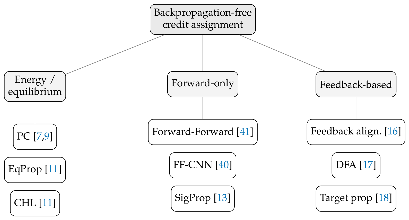
Figure 2.
Block-level contrast. (a) Backpropagation runs a forward pass, stores every activation, then propagates an exact error backward through the whole network (dashed). (b) Local equilibrium learning relaxes all states to a fixed point (bidirectional arrows) and updates each weight from purely local quantities (), with no backward pass and no stored graph. The two coincide in the small-nudge limit (Theorem 2).
Figure 2.
Block-level contrast. (a) Backpropagation runs a forward pass, stores every activation, then propagates an exact error backward through the whole network (dashed). (b) Local equilibrium learning relaxes all states to a fixed point (bidirectional arrows) and updates each weight from purely local quantities (), with no backward pass and no stored graph. The two coincide in the small-nudge limit (Theorem 2).
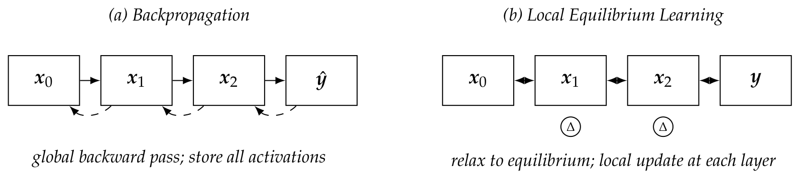
Figure 3.
Predictive-coding microcircuit. Value neurons (circles) hold the states ; error neurons (squares) hold the prediction residuals . Solid arrows are the forward predictions that compute errors; dashed arrows are the local error signals that drive the relaxation and the Hebbian weight update (Lemma 1). Every quantity a synapse needs is available locally, unlike backpropagation’s transposed backward pathway.
Figure 3.
Predictive-coding microcircuit. Value neurons (circles) hold the states ; error neurons (squares) hold the prediction residuals . Solid arrows are the forward predictions that compute errors; dashed arrows are the local error signals that drive the relaxation and the Hebbian weight update (Lemma 1). Every quantity a synapse needs is available locally, unlike backpropagation’s transposed backward pathway.
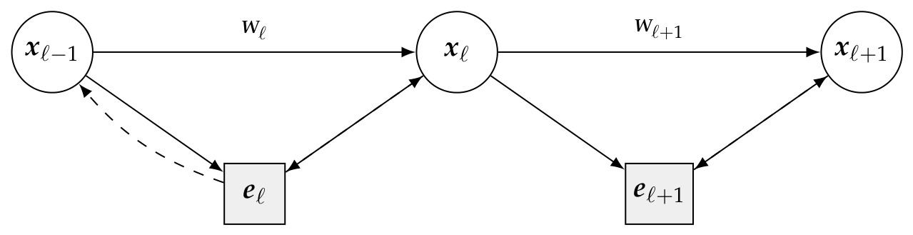
Figure 4.
Equilibrium propagation. The network first relaxes with the output free (state ), then with the output gently nudged toward the target by (state ). The local weight change is proportional to the difference between the two equilibria and, as , equals the backpropagation gradient, using one circuit and only local quantities.
Figure 4.
Equilibrium propagation. The network first relaxes with the output free (state ), then with the output gently nudged toward the target by (state ). The local weight change is proportional to the difference between the two equilibria and, as , equals the backpropagation gradient, using one circuit and only local quantities.
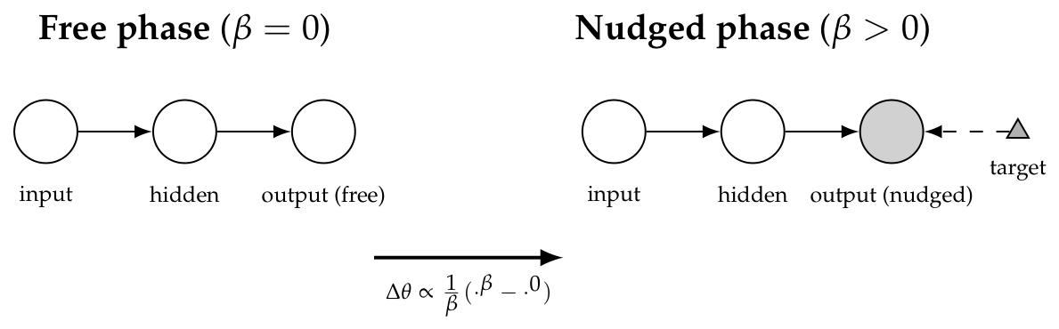
Figure 5.
The spectrum of error locality. Methods are ordered by how much of an explicit error signal they propagate, from backpropagation’s exact global error to forward-only learning’s none. Moving rightward trades gradient fidelity for locality, parallelism and compatibility with in-memory/neuromorphic hardware; LEL sits in the energy-based middle.
Figure 5.
The spectrum of error locality. Methods are ordered by how much of an explicit error signal they propagate, from backpropagation’s exact global error to forward-only learning’s none. Moving rightward trades gradient fidelity for locality, parallelism and compatibility with in-memory/neuromorphic hardware; LEL sits in the energy-based middle.

Figure 6.
The three continual-learning scenarios [20], illustrated on Split-MNIST. Difficulty grows left to right with how much the model must resolve at test time; class-incremental learning, our primary metric, additionally requires calibrating outputs across tasks, the regime where regularization methods fail.
Figure 6.
The three continual-learning scenarios [20], illustrated on Split-MNIST. Difficulty grows left to right with how much the model must resolve at test time; class-incremental learning, our primary metric, additionally requires calibrating outputs across tasks, the regime where regularization methods fail.
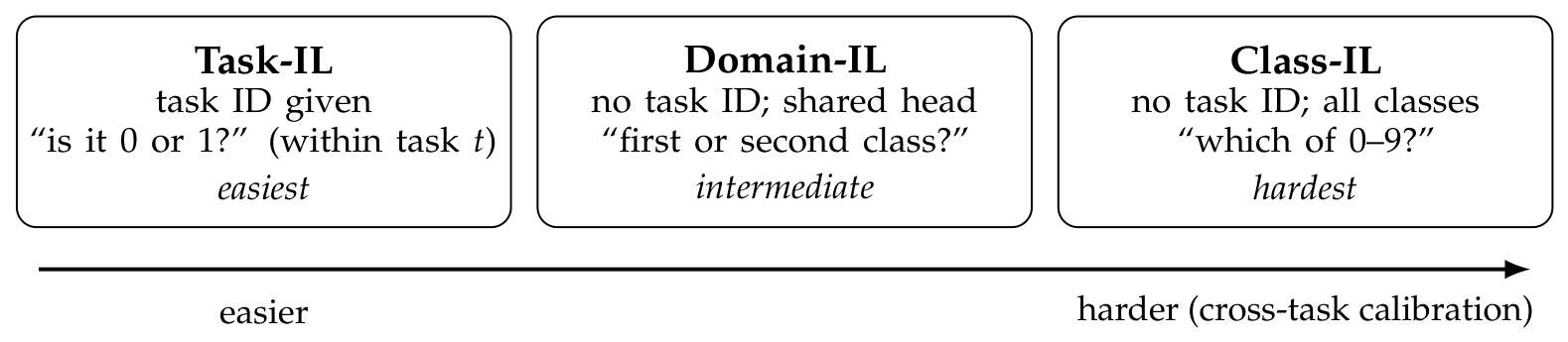
Figure 7.
The LEL train-time loop. With input and output clamped, the network iterates error computation and state relaxation T times to an equilibrium (the inner loop), after which a single local Hebbian update is applied. There is no backward pass; the equilibrium itself performs the credit assignment (Theorem 1).
Figure 7.
The LEL train-time loop. With input and output clamped, the network iterates error computation and state relaxation T times to an equilibrium (the inner loop), after which a single local Hebbian update is applied. There is no backward pass; the equilibrium itself performs the credit assignment (Theorem 1).
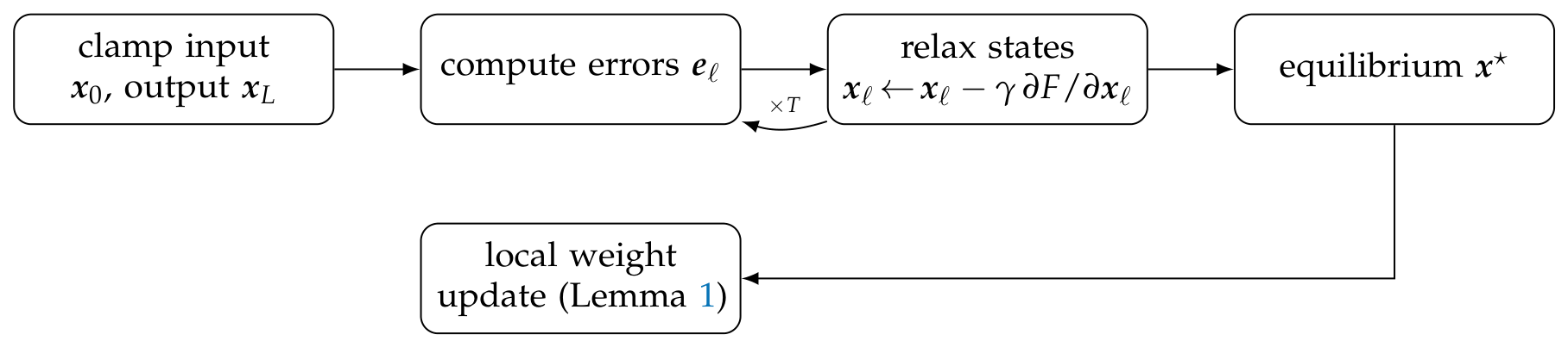
Figure 8.
Numerical validation of Theorem 2 on a network. As the nudge , the cosine between the local update and the negative backpropagation gradient rises monotonically to ; with a fully clamped output the same rule instead descends the free energy E and saturates near . The equivalence to backpropagation is thus a limit, not the default operating point.
Figure 8.
Numerical validation of Theorem 2 on a network. As the nudge , the cosine between the local update and the negative backpropagation gradient rises monotonically to ; with a fully clamped output the same rule instead descends the free energy E and saturates near . The equivalence to backpropagation is thus a limit, not the default operating point.
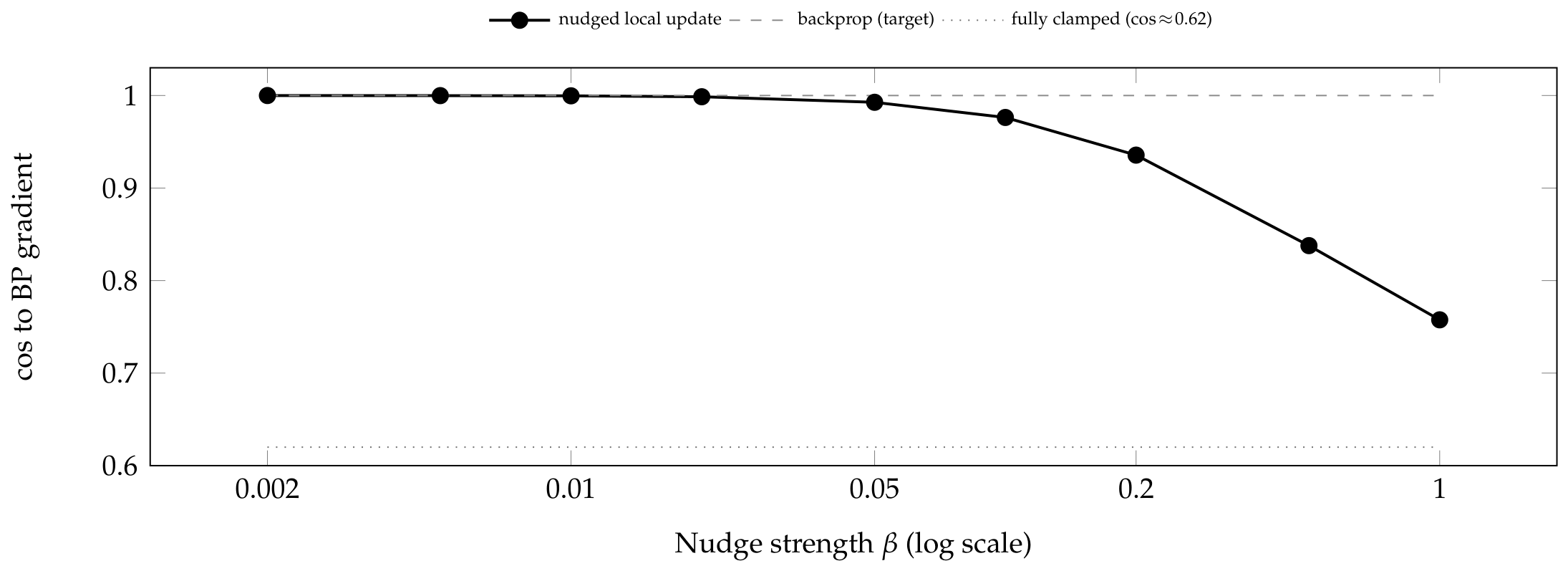
Figure 9.
The continual-learning “dreaming” pipeline. After task A the classifier and per-class generators are frozen; when learning task B, the frozen generators synthesise pseudo-samples of past classes, label them with the frozen classifier, and mix them with the new data. No raw data of past tasks is stored, and every step uses local (backpropagation-free) updates.
Figure 9.
The continual-learning “dreaming” pipeline. After task A the classifier and per-class generators are frozen; when learning task B, the frozen generators synthesise pseudo-samples of past classes, label them with the frozen classifier, and mix them with the new data. No raw data of past tasks is stored, and every step uses local (backpropagation-free) updates.
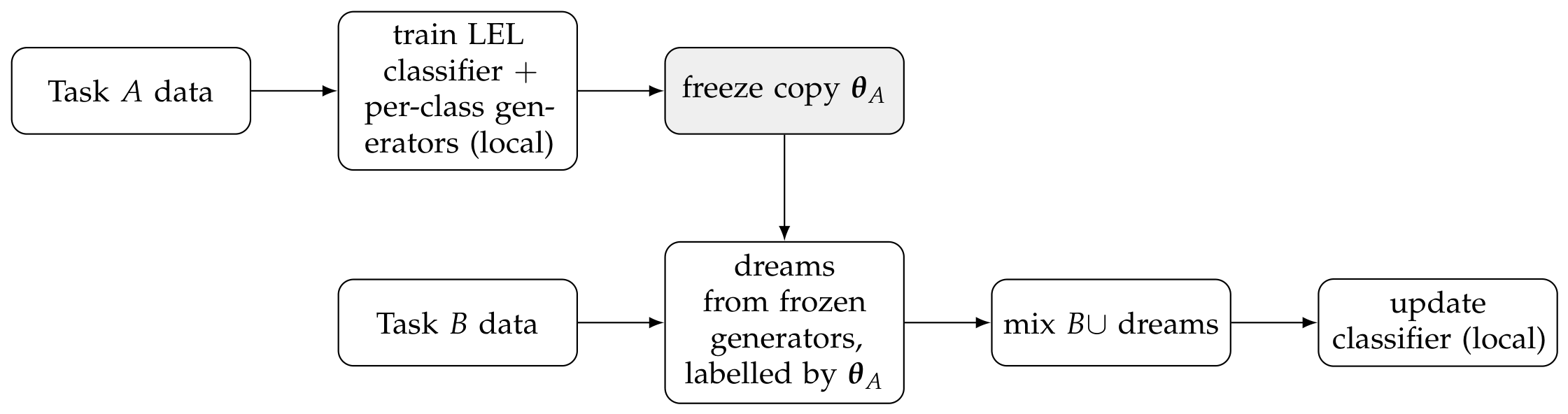
Figure 15.
Generator capacity bounds retention. Class-incremental accuracy on Split-MNIST as a function of the linear generator’s subspace dimension k. Retention grows monotonically with generator fidelity and saturates near the oracle; even far exceeds vanilla learning, and already matches the nonlinear generator. The continual mechanism is not the bottleneck, the generator is.
Figure 15.
Generator capacity bounds retention. Class-incremental accuracy on Split-MNIST as a function of the linear generator’s subspace dimension k. Retention grows monotonically with generator fidelity and saturates near the oracle; even far exceeds vanilla learning, and already matches the nonlinear generator. The continual mechanism is not the bottleneck, the generator is.
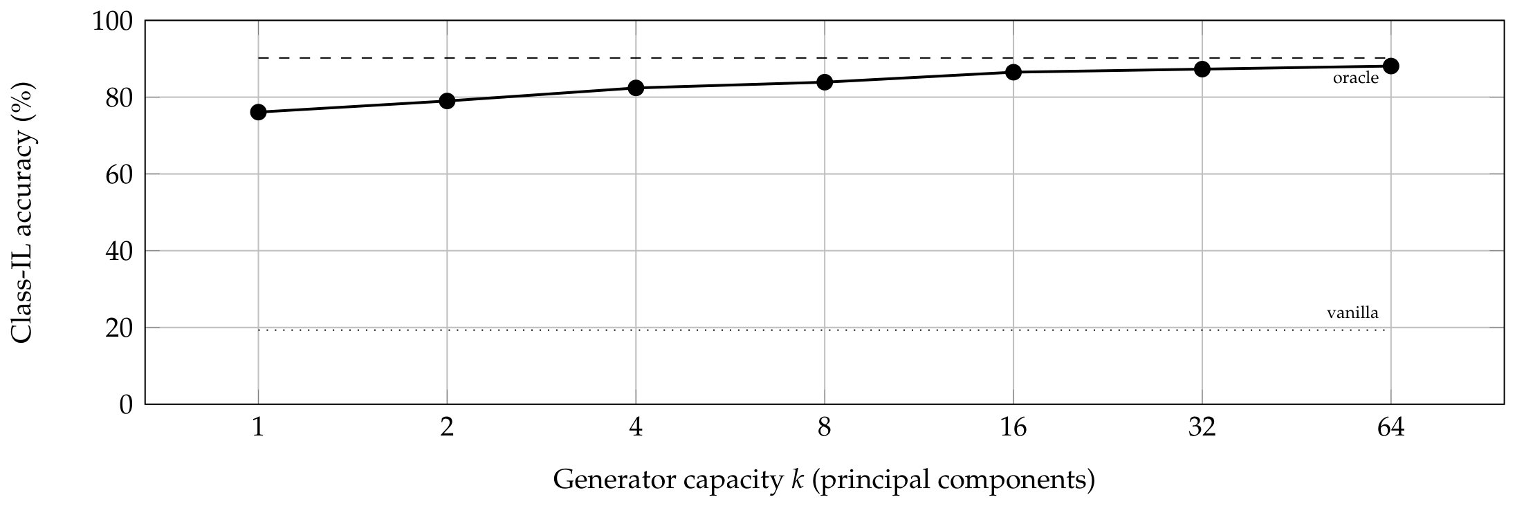
Figure 16.
Generality across datasets. Local generative dreaming recovers the large majority of the joint-training ceiling on every dataset (, and for MNIST, Fashion-MNIST and CIFAR-10), far above the vanilla baseline. On CIFAR-10 the ceiling itself is low, a limit of the shallow pixel classifier, not of the continual mechanism.
Figure 16.
Generality across datasets. Local generative dreaming recovers the large majority of the joint-training ceiling on every dataset (, and for MNIST, Fashion-MNIST and CIFAR-10), far above the vanilla baseline. On CIFAR-10 the ceiling itself is low, a limit of the shallow pixel classifier, not of the continual mechanism.
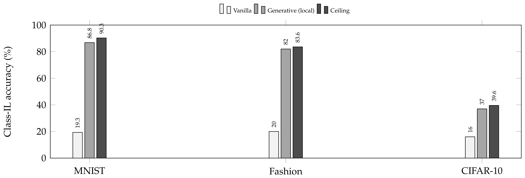
Figure 19.
Why locality matters for energy. (a) On von Neumann hardware, weights and activations are shuttled between memory and compute, and this data movement, not the arithmetic, dominates the energy budget [4]; backpropagation worsens it by storing the activation graph and transporting transposed weights. (b) In an analog crossbar the weight is the device, so the multiply–accumulate happens in place and local rules update it without moving data, the regime where energy-based local learning is projected to gain orders of magnitude [12,45].
Figure 19.
Why locality matters for energy. (a) On von Neumann hardware, weights and activations are shuttled between memory and compute, and this data movement, not the arithmetic, dominates the energy budget [4]; backpropagation worsens it by storing the activation graph and transporting transposed weights. (b) In an analog crossbar the weight is the device, so the multiply–accumulate happens in place and local rules update it without moving data, the regime where energy-based local learning is projected to gain orders of magnitude [12,45].
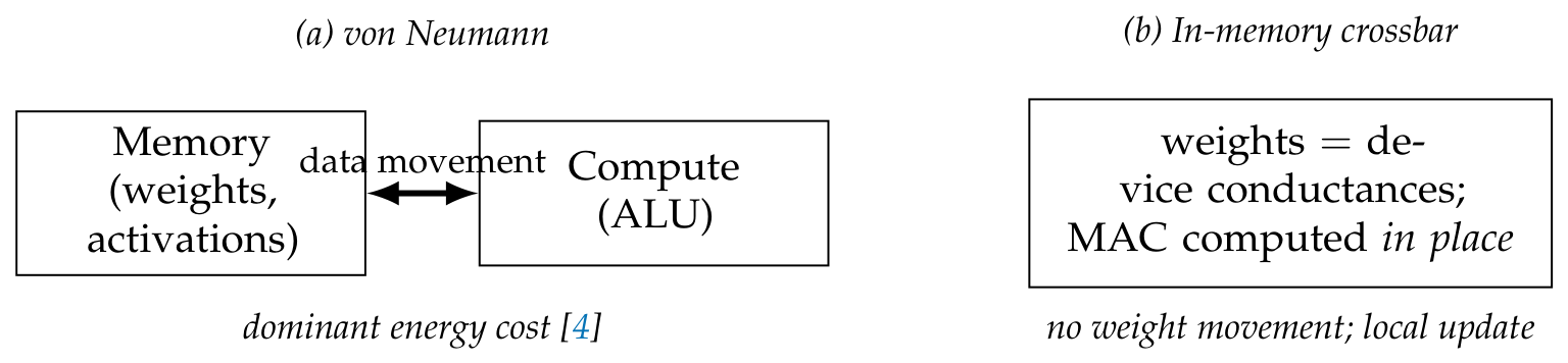
Table 1.
Qualitative comparison of credit-assignment families. “Local” means each update uses only quantities at the two neurons a synapse connects; “recovers BP” means the update equals the backpropagation gradient in a limit.
Table 1.
Qualitative comparison of credit-assignment families. “Local” means each update uses only quantities at the two neurons a synapse connects; “recovers BP” means the update equals the backpropagation gradient in a limit.
| Family | Local | Recovers BP | Activation | Neuromorphic | Scales to |
|---|---|---|---|---|---|
| update | memory | fit | deep nets | ||
| Backpropagation [1] | no | , | poor | yes | |
| Predictive coding [9] | yes | yes () | good | hard (active) | |
| Equilibrium prop. [11] | yes | yes () | strong | hard (active) | |
| Contrastive Hebbian [11] | yes | yes | good | limited | |
| Forward-Forward [41] | yes | no | good | emerging | |
| Feedback alignment [16] | partial | approx. | medium | limited | |
| Target propagation [18] | partial | approx. | medium | limited |
Table 2.
Comparison of continual-learning methods. “Class-IL” summarises the reported behaviour in the class-incremental scenario under the assumptions listed in the table; “BP-free” marks methods whose main credit-assignment step does not require backpropagation. The last row is the strategy benchmarked in this review.
Table 2.
Comparison of continual-learning methods. “Class-IL” summarises the reported behaviour in the class-incremental scenario under the assumptions listed in the table; “BP-free” marks methods whose main credit-assignment step does not require backpropagation. The last row is the strategy benchmarked in this review.
| Method | Family | Stores data | Generative | BP-free | Class-IL |
|---|---|---|---|---|---|
| EWC [21] | regularization | no | no | no | poor |
| SI [22] | regularization | no | no | no | poor |
| MAS [23] | regularization | no | no | no | poor |
| LwF [56] | distillation | no | no | no | poor |
| iCaRL [26] | exemplar | yes | no | no | moderate |
| GEM [57] | exemplar | yes | no | no | good |
| Experience replay | exemplar | yes | no | no | good |
| DGR [24] | gen. replay | no | yes (BP) | no | good |
| Brain-inspired replay [25] | gen. replay | no | yes (BP) | no | strong |
| Pseudo-rehearsal [24] | gen. replay | no | noise | no | poor (high-dim) |
| PackNet [58] | architecture | no | no | no | task-IL |
| Context gating [27] | architecture | no | no | no | task-IL |
| LEL + dreaming (this study) | gen. replay | no | yes (local) | yes | effective under the reported Split-MNIST/Fashion-MNIST protocol |
Table 3.
Three levels that must be kept separate when studying backpropagation-free continual learning. Many apparent disagreements in the literature come from mixing these levels rather than from genuine algorithmic disagreement.
Table 3.
Three levels that must be kept separate when studying backpropagation-free continual learning. Many apparent disagreements in the literature come from mixing these levels rather than from genuine algorithmic disagreement.
| Level | Examples | Question it answers |
|---|---|---|
| Credit assignment | Backpropagation, predictive coding, EqProp, LEL, feedback alignment, target propagation, forward-only learning | How does a parameter know whether and how to change? |
| Continual mechanism | EWC, SI, MAS, LwF, replay, generative replay, architectural isolation, gating | How is old knowledge protected or rehearsed while learning new tasks? |
| Evaluation protocol | Task-IL, Domain-IL, Class-IL; Split-MNIST, Split-Fashion-MNIST, Split-CIFAR; joint and oracle bounds | What must the model decide at test time, and what resources were allowed during training? |
Table 4.
Design patterns for constructing a backpropagation-free continual learner. Each row identifies a component that can be changed independently, together with the main diagnostic that should accompany the change.
Table 4.
Design patterns for constructing a backpropagation-free continual learner. Each row identifies a component that can be changed independently, together with the main diagnostic that should accompany the change.
| Component | Typical choices | Diagnostic to report |
|---|---|---|
| Inference dynamics | clamped predictive-coding relaxation, nudged EqProp-style relaxation, incremental/parallel activity updates | Energy decrease, equilibrium residuals, number of steps to stability and sensitivity to the state step size |
| Synaptic update | Hebbian local error rule, contrastive difference, forward-only local objective, feedback-aligned local target | Whether the update is truly local and whether it aligns with backpropagation in the relevant limit |
| Retention mechanism | no defence, quadratic anchoring, replay, generative dreaming, task gating | Final accuracy and forgetting under Task-IL and Class-IL, not only one scenario |
| Memory policy | no data, compact statistics, generator parameters, feature buffers, raw exemplars | Exact number and type of stored quantities per class or per task |
| Generator | Oja/PCA subspace, local autoencoder, energy sampler with prior, associative memory | Sample fidelity, oracle gap, and whether generated samples remain on the data manifold |
| Calibration | single head, multi-head, task-conditioned output, nearest-mean classifier | Whether cross-task scores are comparable without task identity |
| Hardware substrate | CPU/GPU simulation, analog crossbar, spiking neuromorphic processor, mixed-signal prototype | Measured latency and joules, separated from projected operation counts |
Table 5.
A benchmark ladder for backpropagation-free continual learning. Moving upward adds one major difficulty at a time, making failures easier to diagnose.
Table 5.
A benchmark ladder for backpropagation-free continual learning. Moving upward adds one major difficulty at a time, making failures easier to diagnose.
| Rung | Benchmark | Purpose | Failure it exposes |
|---|---|---|---|
| 1 | Two-moons or low-dimensional toy tasks | Verify local learning and forgetting under controlled geometry | Under-training mistaken for retention |
| 2 | Single-task MNIST/Fashion | Check stationary accuracy against a matched backpropagation model | Base local learner too weak |
| 3 | Split-MNIST Class-IL | Test cross-task calibration and replay under a standard protocol | Regularization collapse and last-task bias |
| 4 | Generator-capacity ablation | Separate replay from generator fidelity | Poor samples blamed on continual learning |
| 5 | Split-Fashion-MNIST and raw-pixel CIFAR-10 | Probe dataset transfer and base-classifier ceiling | Low absolute accuracy caused by weak representation |
| 6 | Feature-space Class-IL | Test whether local replay works when representation quality improves | Hidden dependence on raw-pixel generators |
| 7 | Deep local networks | Test whether depth remedies balance equilibrium errors | Vanishing local error in early layers |
| 8 | Hardware-in-the-loop replay | Measure energy and latency in the intended substrate | Energy advantage that exists only on paper |
Table 6.
Analytical per-update scaling for an L-layer network of width w and batch size m. “Weight transport” marks whether a transposed copy of the forward weights is required to assign credit; “locality” whether each update uses only quantities at the two neurons a synapse connects.
Table 6.
Analytical per-update scaling for an L-layer network of width w and batch size m. “Weight transport” marks whether a transposed copy of the forward weights is required to assign credit; “locality” whether each update uses only quantities at the two neurons a synapse connects.
| Quantity | Backpropagation | LEL (this study) |
|---|---|---|
| Compute / update | ||
| Passes over the net | 1 forward backward | T relaxation steps |
| Activation memory | ||
| Weight transport | required | none |
| Locality of update | no (global signal) | yes (Lemma 1) |
| Parallelism over layers | sequential | layers relax in parallel |
| Generative direction | none | native (same network) |
Table 7.
Map of the empirical case study: each experiment, its script and headline finding.
| Experiment | Script | Finding |
|---|---|---|
| Local vs. backprop | equilibriumvsbackprop.py | local rule learns non-linear task ( vs. ) |
| Theorem validation | theoremvalidation.py | cosine to backprop as nudge |
| Continual (binary) | mnistcontinualdream.py | noise replay fails off-manifold; generative works |
| Manifold () | manifolddreamlel.py | on-manifold dreams eliminate forgetting |
| Full Split-MNIST | fullsplitmnist.py | class-IL vs. vanilla/EWC/SI |
| Seeds/scenarios/ablation | reinforce.py | (5 seeds); task-IL |
| Generalisation | fashioncontinual.py, cifarcontinual.py | Fashion ; CIFAR |
| Baselines | baselinesewc.py, baselinessi.py | EWC/SI (class-IL) |
| Depth problem | deepleltestbed.py | six-order error imbalance at |
| Efficiency | measureefficiency.py, energyestimate.py | more compute; energy projection |
Table 8.
Representative hyperparameters in the released experiments. The purpose is reproducibility and diagnosis, not exhaustive tuning. Symbols match Algorithms 1 and 2.
Table 8.
Representative hyperparameters in the released experiments. The purpose is reproducibility and diagnosis, not exhaustive tuning. Symbols match Algorithms 1 and 2.
| Component | Default | Role in the study |
|---|---|---|
| Classifier width | on MNIST/Fashion, on CIFAR-10 | Keeps the architecture shallow and transparent while giving enough capacity for the continual mechanism to be tested |
| Classifier relaxation | in the main Split-MNIST runs | Assigns credit by state relaxation; ablated explicitly in Figure 11 |
| State step size | on MNIST/Fashion, smaller on CIFAR-10 | Controls stability of the inference dynamics, especially in high-dimensional inputs |
| Classifier epochs | 35 for Split-MNIST main runs | Trains each task enough to avoid the under-training artefact |
| Dreams per old class | in the main result | Main replay budget; swept in Figure 10 |
| Generator type | nonlinear local PC autoencoder or Oja/PCA subspace | Tests whether retention is limited by generator fidelity rather than by replay itself |
| Evaluation subset | first 400 test examples per class in several scripts | Keeps runtime small and identical across methods |
| Seeds | 0–4 for the headline Split-MNIST result | Reports mean and dispersion for the central claim |
Table 9.
Memory policy of the methods compared in the empirical study. The distinction between model memory and data memory is essential when interpreting “storage-free” continual learning.
Table 9.
Memory policy of the methods compared in the empirical study. The distinction between model memory and data memory is essential when interpreting “storage-free” continual learning.
| Method | Stored after each task | Interpretation |
|---|---|---|
| Vanilla LEL | current classifier parameters | No explicit protection against forgetting |
| EWC / SI | classifier parameters plus importance or path statistics | No raw data, but still backpropagation-based credit assignment |
| Oracle replay | selected real images from old tasks | Upper bound on what replay could achieve with perfect memory |
| Noise replay | random inputs and labels from the old classifier | Storage-free but off-manifold in high dimension |
| Local dreaming | per-class local generator parameters or compact subspace statistics | Storage-free with respect to raw data; rehearsal samples are generated on demand |
Table 10.
Class-incremental Split-MNIST (single 10-way head; chance ). Ceiling = joint training; oracle = replay of stored real images.
Table 10.
Class-incremental Split-MNIST (single 10-way head; chance ). Ceiling = joint training; oracle = replay of stored real images.
| Method | Final acc. (10 classes) |
|---|---|
| Ceiling (joint training) | |
| Oracle (real-image replay) | |
| Vanilla (no defence) | |
| Backprop + EWC [21] (any ) | |
| Backprop + SI [22] (best ) | |
| Noise replay [24] | |
| Generative dreaming (local) |
Table 11.
Honest comparison of LEL against backpropagation (BP).
| Axis | Backpropagation | LEL (this study) |
|---|---|---|
| Raw accuracy (i.i.d.) | (MNIST MLP) | , matches |
| Class-IL continual (vs. EWC/SI) | , surpasses | |
| Speed / compute (von Neumann) | – worse, lags | |
| Activation memory | , better | |
| Neuromorphic energy | not portable | projected – lower |
| Biological plausibility | low (weight transport) | high (local), better |
| Very deep networks | mature | open problem, lags |
Table 12.
Class-incremental generative dreaming across datasets (all local, no backprop).
| Dataset | Ceiling | Vanilla | Dreaming (local) |
|---|---|---|---|
| Split-MNIST [20] | (96% ceil.) | ||
| Split-Fashion-MNIST [35] | (98% ceil.) | ||
| Split-CIFAR-10 [65] | (93% ceil.) |
Table 13.
Single-task MNIST accuracy versus depth (width 128, trained from scratch with the local rule). The monotone decline is the accuracy-side signature of the error-imbalance barrier.
Table 13.
Single-task MNIST accuracy versus depth (width 128, trained from scratch with the local rule). The monotone decline is the accuracy-side signature of the error-imbalance barrier.
| Hidden layers D | 1 | 2 | 3 | 4 | 6 | 8 |
|---|---|---|---|---|---|---|
| Test accuracy (%) |
Table 14.
Efficiency of a network (per training sample). On von Neumann hardware LEL costs more; the energy advantage is a projection on in-memory substrates using the figures of [4].
Table 14.
Efficiency of a network (per training sample). On von Neumann hardware LEL costs more; the energy advantage is a projection on in-memory substrates using the figures of [4].
| Metric | Backprop | LEL (this study) |
|---|---|---|
| Relative compute (vs. forward) | () | |
| Wall-clock (CPU, same epochs) | slower | |
| Activation memory | ||
| Energy, von Neumann (DRAM) | µJ | µJ (worse) |
| Energy, in-memory (projected) | , | –3 µJ |
Table 15.
Open questions organised as testable research tasks. The table is intended as a starting point for new projects rather than as a complete forecast of the field.
Table 15.
Open questions organised as testable research tasks. The table is intended as a starting point for new projects rather than as a complete forecast of the field.
| Problem | Near-term test | Evidence of progress |
|---|---|---|
| Depth and scaling | Train deeper LEL/PC networks while monitoring per-layer equilibrium errors | Error magnitudes remain balanced and accuracy improves with added depth |
| Generator quality | Swap local generators under a fixed replay protocol | Class-IL accuracy approaches the oracle without storing raw data |
| Feature-space replay | Run local continual learning on learned or frozen representations | Higher CIFAR-like ceilings without changing the continual mechanism |
| Attention | Formulate local updates for attention-like retrieval | Sequence or transformer-style benchmark trained without a global backward pass |
| Hardware | Implement relaxation and dreaming on neuromorphic or in-memory hardware | Measured joule advantage, not only projected operation counts |
| Memory accounting | Report raw data, feature data, generator and statistic budgets separately | Fair comparison between replay, regularization and architecture methods |
| Evaluation culture | Publish failures and controls alongside positive numbers | Fewer irreproducible claims and clearer design boundaries |
Disclaimer/Publisher’s Note: The statements, opinions and data contained in all publications are solely those of the individual author(s) and contributor(s) and not of MDPI and/or the editor(s). MDPI and/or the editor(s) disclaim responsibility for any injury to people or property resulting from any ideas, methods, instructions or products referred to in the content. |
© 2026 by the authors. Licensee MDPI, Basel, Switzerland. This article is an open access article distributed under the terms and conditions of the Creative Commons Attribution (CC BY) license (http://creativecommons.org/licenses/by/4.0/).
Copyright: This open access article is published under a Creative Commons CC BY 4.0 license, which permit the free download, distribution, and reuse, provided that the author and preprint are cited in any reuse.


