

Submitted:
07 July 2026
Posted:
08 July 2026
You are already at the latest version
Abstract
Alignments explain, event by event, how an observed trace deviates from a process model. Computing an optimal alignment, however, requires exact shortest-path search over a synchronous product, which degrades with concurrency, loops, duplicate labels, and invisible transitions, precisely the ingredients of real discovered models. Purely learned aligners are fast but untrustworthy: their output may be illegal or silently suboptimal. This paper introduces LARA (Learned Adaptive Recombined Alignments), a hybrid system in which a neural model proposes and an exact layer verifies. The neural model is a small foundation model for alignment: trained once, offline, on synthetic data, it is vocabulary-free and applies to any net and any log without per-log training or configuration. Its scores drive a constrained decoder, and exact replay checks every candidate, so the output is always a legal alignment with a known cost; on demand, the exact backend upgrades it to a certified optimal one. In the assessment, every produced alignment is legal, and the large majority attains the exact optimal cost. A guidance ablation attributes the learned contribution specifically to duplicate-label resolution, the sub-problem where purely structural heuristics are blind. Legality transfers zero-shot to unseen net families and to real-life event logs, and the learned fast path overtakes exact search on larger synthetic nets and on a real discovered model dominated by invisible transitions.
Keywords:
process mining
; conformance checking
; alignments
; Petri nets
; neural networks
; certification
1. Introduction
Process mining relates recorded event data to process models in order to discover, check, and improve processes [25]. Conformance checking quantifies how well observed behavior agrees with modeled behavior [8,19], and alignments are its reference technique [1,2]: an alignment explains every event of a trace through synchronous, log, and model moves, and an optimal alignment minimizes the total deviation cost. The result is not merely a fitness number but a diagnostic object showing exactly where log and model disagree.
The guarantee of optimality is also the burden of the technique. Optimal alignments are computed by exact shortest-path search, typically A* [13] with heuristics derived from the marking equation [27,28], over the reachability graph of a synchronous product net. This state space grows quickly with concurrency, loops, duplicate labels, and invisible transitions, and the problem is intrinsically hard [21]. These are exactly the ingredients of discovered models, so exact alignment is often the bottleneck of the entire analysis, with running times that cannot be predicted from the input size.
Machine learning promises speed, and neural models have been applied successfully to event data for predictive monitoring and discovery [7,22,23]. However, a purely learned aligner is unusable for conformance checking: a predicted alignment may be illegal, meaning its model projection cannot be replayed from the initial to the final marking, or it may be silently suboptimal, and any conformance verdict built on it inherits this uncertainty. The tension is between trust and tractability.
This paper asks whether the tension can be dissolved instead. We present LARA (Learned Adaptive Recombined Alignments), a neural-guided alignment system built around one invariant: neural output is never trusted as a certificate. A learned model scores alignment decisions; a constrained greedy decoder turns the scores into a candidate whose model moves are fireable by construction; an exact replay verifier decides legality; and an exact alignment backend remains the sole authority on optimality, certifying or repairing the candidate. Speed comes from the model, but correctness never depends on it: the system degrades from certified optimal to a safe upper bound, never to wrong. Figure 1 summarizes the learned core of the approach and the outputs it offers.
For the user of conformance checking, this design is interesting for three reasons. First, the neural component is a small foundation model for alignment: trained once, offline, on synthetic data, and vocabulary-free through hashed label embeddings, it applies to any event log and any Petri net without retraining or configuration. Second, its per-trace latency is dominated by a fixed forward pass, staying flat and predictable where exact search has heavy tails, which is what interactive analysis of large discovered models needs. Third, adopting it is risk-free: every answer is at least a legal alignment with a verified cost, and in certified mode exactly as trustworthy as classical alignment. The contribution of the paper is this foundation model for alignment, one small neural model that scores alignment moves for any Petri net and any event log and is designed to resolve duplicate labels and invisible routing, the classic hard cases of alignment, together with the certifying architecture that makes it safe to adopt (Section 4), the exact-labeled synthetic pipeline that trains it, and an assessment asking what learning adds over pure search, when the fast path overtakes exact A*, and whether one checkpoint transfers unchanged to real-life logs (Section 5).
The central question, can a learned model make trace alignment fast without making it less trustworthy, is refined into six research questions. RQ1 (legality): are the produced alignments always legal, even on unseen nets and vocabularies? RQ2 (near-optimality): how often is the exact optimal cost attained, and how large are the gaps otherwise? RQ3 (ambiguity): are duplicate labels and invisible routing resolved? RQ4 (generalization): does performance transfer across families, scales, and real-life logs? RQ5 (certification): how often does cost equality certify the candidate? RQ6 (attribution): how much quality is owed to the learned scores rather than to the constrained search around them?
2. Related Work
Foundations and alignments. Petri nets [16] remain central to conformance checking [8,25]. Replay-based conformance checking links trace events to model elements [19]; cost-based alignments [1,2] introduced the synchronous, log, and model move vocabulary used throughout this paper, and van Zelst et al. [28] formalize alignment computation as a shortest-path problem over a synchronous product. LARA preserves this diagnostic tradition: its output is an alignment object with transition identities, not a predicted score.
Exact search and acceleration. Efficient exact methods refine A* [13] with (extended) marking-equation heuristics [27] or reduce explored states as in REACH [9]; complexity analyses underline why the problem resists such optimizations in general [21]. These approaches provide formal guidance inside one search; LARA instead provides empirical guidance outside the exact search and keeps the exact layer for certification only.
Decomposition and recomposition. Decomposing nets speeds up conformance checking [24], local alignments can be merged [30], recomposition restores exact results or bounds [14], and automata with S-components offer another scalable route [18]. LARA is architecturally close to this family, but its regions are latent and trace-dependent rather than fixed structural decompositions.
Approximate conformance checking. Token-based replay [4,19], alignment approximation for process trees [20], and relaxation labeling [17] occupy the same speed and accuracy space as LARA’s fast mode. The distinctive feature of LARA is the certification boundary: candidates are replay-verified, then certified by cost equality or repaired exactly. Neural methods in process mining. Neural models of event data have mostly targeted prediction, with recurrent networks [23], transformers [7,29], and graph neural networks for discovery [22]; a recent survey identifies conformance checking as an open opportunity for AI [12]. None of these works constructs legal, costed alignments against an explicit Petri net; LARA is a concrete instance of that agenda.
Learning-augmented search. Outside process mining, machine learning guides combinatorial optimization [3] and shortest-path search, as in Neural A* [31]. LARA is deliberately more conservative: learned scores rank moves for a greedy decoder and are never used as admissible heuristics, so the trust model of exact conformance checking is preserved. The gap LARA addresses is thus certifiable neural guidance for Petri net trace alignment.
3. Preliminaries
Events, traces, and logs. Let be a finite alphabet of activity labels. A trace is a finite sequence of events describing one case; an event log is a multiset of traces. We align a single trace against a model; log-level results follow by aggregation.
Labeled Petri nets. A Petri net is a tuple with places P, transitions T, , and flow relation . A marking assigns tokens to places; a transition is enabled iff all its input places carry a token, and firing it consumes from input and produces into output places, written . A labeling function marks transitions as visible or invisible (); invisible transitions represent routing that leaves no trace in the log, and two distinct transitions may share a visible label (duplicate labels). Both phenomena are central here: an observed event determines the label of a matching transition but not its identity. A system net adds initial and final markings.
Alignments. Let ≫ denote a skip symbol. A move is a pair , excluding : a synchronous move with , a log move , or a model move . An alignment of and is a sequence of moves such that (1) the sequence of non-≫ log components equals exactly, and (2) the sequence of non-≫ model components is a firing sequence of N from that reaches . An alignment satisfying both conditions is legal. Moves carry the transition identity t, not just its label: with duplicate labels, two alignments can have identical label projections yet fire different transitions.
Costs and optimality. The standard unit cost model charges 0 for synchronous moves and invisible model moves and 1 for log moves and visible model moves. The cost of an alignment is , and an alignment is optimal iff its cost equals . Optimal alignments need not be unique; the optimal cost is, and under unit costs it counts the minimum number of deviations needed to explain the trace.
Synchronous product and A*. The classical construction builds a synchronous product of and a linear trace net; legal alignments correspond exactly to complete firing sequences of the product, so computing an optimal alignment is a shortest-path problem over its reachability graph [28], solved by A* with admissible heuristics from the (extended) marking equation [27]. We use the state-equation A* aligner of PM4Py [5] as exact backend and as the source of ground-truth labels.
Certification. A certificate of optimality for a candidate is a proof that . Two routes provide such a proof: the marking equation yields a lower bound on [27], so a legal candidate whose cost meets this bound is optimal without any search, and the exact solver returns itself, so cost equality certifies a legal candidate even if it differs from the exact alignment. The paper uses cost equality as its certification rule.
4. Approach
LARA separates candidate generation (learned, fast, uncertified) from certification (exact, trusted). Figure 2 shows the pipeline. At alignment time a net and trace pair passes through three stages, each consuming exactly what the previous one produces: input encoding re-encodes the pair for the neural model (Section 4.1), the neural model scores the possible moves (Section 4.2), and the decoder turns the scores into one alignment that exact methods then verify and certify (Section 4.3). Section 4.4 and Section 4.5 describe the offline training of the neural model, which happens once and is amortized over all later use.
4.1. Input Encoding: Reading the Net and the Trace
Input: a system net and a trace of length n. Output: a graph view of the net, the trace as a sequence of label identifiers, and a compatibility mask C recording which event and transition pairs share a label.
The net as a typed graph. The net is encoded as a bipartite graph with one node per place and one node per transition. Encoding the net itself, rather than any behavioral expansion of it, keeps the input linear in the size of the net; the reachability graph, whose potentially exponential size is what makes exact alignment expensive, is never materialized. The node attributes are chosen so that every quantity the move scorer must weigh is locally visible. Place nodes carry their token counts in the initial and final markings and their degrees: the markings tell the model where execution starts and where it must end, and the degrees mark branching and synchronization points. Transition nodes carry their invisibility flag and their move costs, since inserting a is free while a visible model move is penalized, together with their degrees and a self-loop context flag, which signal local choice, concurrency, and repeatable behavior. Every arc contributes two edges, one per direction, with the direction recorded as the edge type. Keeping direction observable preserves the firing semantics: an undirected edge could not distinguish a preset place, which enables a transition, from a postset place, which receives its tokens. The reverse edges are added because the information that distinguishes two transitions sharing a label typically lies downstream of them, for example in the branch suffix that follows each. If messages flowed only along arc direction, two duplicates with symmetric presets would receive provably identical representations; with edges in both directions, the disambiguating suffix reaches each duplicate in two hops (Section 5.3).
Activity labels without a vocabulary. Activity labels are mapped to a bounded set of 8,192 identifiers by a stable hash (BLAKE2b), one identifier being reserved for ; the trace becomes its sequence of hashed identifiers. The model therefore never memorizes activity names, so one trained checkpoint applies unchanged to logs whose vocabularies it has never seen, the prerequisite for a foundation model across event logs (Section 5.6). An event and a transition with the same label receive the same identifier, which ties trace positions to their candidate transitions. The boolean mask C, with iff event i and transition j carry the same visible label, later guarantees that only label-consistent synchronous moves can be proposed.
4.2. Neural Scoring: Three Questions per Net and Trace Pair
Input: the encoded pair of Section 4.1. Output: scored answers to the three questions any aligner faces. For every event i and transition j: how plausible is it that event i synchronizes with exactly transition j (synchronous scores , masked by C)? For every event: how plausible is it that it is a deviation to be skipped (log-move scores in )? For every transition: how plausible is it that the model requires it although no event matches (model-move scores in )? Only these move scores travel further down the pipeline, to the decoder of Section 4.3. The model is deliberately small, roughly 3M parameters (hidden dimension ), and runs comfortably on CPU.
Two coupled encoders. A graph transformer reads the net: over three rounds, every place and transition refines its representation by attending to all other nodes and exchanging messages with its neighbors, separately per arc type and direction, so structural context accumulates in each node. A sequence transformer [29] reads the trace, embedding events through the same label identifiers as transitions, so an event and its label-compatible transitions start from the same representation. One round of bidirectional cross-attention couples the two encoders: every event looks at the transitions that could explain it, and every transition looks at the events that could justify firing it. This coupling makes all scores trace-dependent: the same net is scored differently depending on where the trace deviates.
Move-scoring heads. The synchronous score of event i and transition j compares their two representations (a scaled bilinear form), hard-masked by C; row i is the model’s belief about which concrete transition event i should synchronize with, and this is where duplicate-label resolution happens. Log-move and model-move scores are read off the event and transition representations directly.
A diagnostic decomposition branch. A learned router additionally assigns transitions and events softly to latent regions, and per region a small head predicts a local deviation sketch (out of patterns), lower and upper cost bounds, and an uncertainty estimate; the summed upper bounds are the model’s estimate of the total alignment cost, supervised against the optimum. Figure 3 illustrates the branch. It is the learned analogue of decomposition-based conformance checking [24,30]: the partition is predicted per net and trace pair rather than fixed structurally. This branch is diagnostic only: its outputs never reach the decoder or the exact search, since a learned cost bound carries no admissibility guarantee.
4.3. Decoding, Verification, and Certification: From Scores to a Certified Alignment
Input: the system net, the trace , and the move scores of Section 4.2. Output: a legal alignment whose guarantee depends on the chosen mode: certified optimal, exactly repaired, or a verified upper bound. The learned scores are consumed exclusively by the decoder; the verifier and certifier judge only the resulting alignment object, so the trust boundary of Figure 2 is crossed by an alignment, never by neural output.
Greedy decoding, guided by the scores. The decoder walks over the trace once, left to right, and always knows the current marking of the net (Figure 4); the diagnostic regions of Section 4.2 play no role here. For each event it must answer one question: which transition, if any, should explain this event? The marking does the coarse work, since only transitions that are enabled and carry the event’s label qualify, and three cases remain. (1) Exactly one transition qualifies: it is fired as a synchronous move, and no learned knowledge is needed. (2) Several qualify, which is precisely the duplicate-label situation: the decoder fires the one with the highest synchronous score; a structural tie-break could only guess between look-alike duplicates, while the score is computed with a view of the entire trace and knows which branch the suffix supports. (3) None qualifies: the net must first catch up. A breadth-first search from the current marking, bounded at depth 8, looks for a short sequence of model moves that enables the event; invisible transitions are tried first and the model-move scores order the remaining options, so the scores again decide which routing path through the net the model most plausibly took. If the search finds nothing, the event becomes a log move, once more without any score. After the last event, a final bounded search (depth 32) appends the model moves that reach . The marking thus forces everything that can be forced, and the learned scores settle exactly the two choices a greedy pass would otherwise have to guess: which duplicate to synchronize with and which routing path to fire. Since every move is fired on the tracked marking, the candidate is fireable by construction.
Scope of the bounded search. Exact aligners explore the synchronous product, may revise any decision, and provably return the cheapest alignment [27,28]; the decoder’s search explores model moves only, stops at the first marking that enables the next event rather than the cheapest one, and never revisits a commitment. It guarantees that the candidate can be replayed, not that it is cheap; this is the failure mode analyzed in Section 5.7 and the reason the exact layer stays in the loop. A precomputed per-net runtime keeps the search cheap, so the neural forward pass dominates fast-mode wall time.
Verifier and certifier. The verifier sees only : it replays the model moves from , checks that is reached and that the log projection equals , and computes . The certifier then delivers the requested guarantee: fast returns the verified candidate with as an upper bound on ; certified additionally runs the exact aligner and either certifies the candidate by cost equality (Section 3) or returns the exact alignment as repair; anytime degrades gracefully on exact-backend timeouts, returning the best available bounds.
4.4. Exact-Labeled Training Data
The scoring heads are trained by imitation, and imitation is only as good as its labels: every training pair must carry a provably optimal alignment with transition identities. Real event logs are a poor source of such labels: the ground truth would still have to be computed by an exact aligner, a log offers no control over how often the hard phenomena (duplicate labels, invisible routing, overlapping deviations) occur, and the instances one would most like to learn from are exactly those where exact labeling is expensive. Synthetic generation turns this around: the generator controls which phenomena the model sees and at which rate, every label is exact by construction, and the supply of data is unlimited. What synthetic data cannot offer, realistic activity names, is irrelevant by design: with the hashed labels of Section 4.1 the model learns structure, never vocabulary, and the zero-shot results of Section 5.6 confirm that this transfer works.
Each example is produced in three steps. First, a net is drawn from a curriculum in which every family is the smallest structure that isolates one of the two learned decisions of Section 4.3, so that the supervision signal for each decision is undiluted: with probability 0.8 a linear workflow over 3 to 8 activities, optionally opened by an invisible transition, on which the model learns where deviations belong, and with probability 0.2 a duplicate-label choice whose two branches start with the same label and differ only in their suffixes, on which identity resolution is learnable precisely because the ambiguous event itself carries no signal. Second, a fitting trace is perturbed with controlled deviations (rate 0.25: deletion, insertion, duplication, swap, append). Third, the exact backend computes an optimal alignment with transition identities and its cost, and every label must additionally pass replay verification, so no incorrect supervision can enter the corpus. The reference corpus is the intentionally compact first stage of this curriculum, 400 training examples (plus 100 validation and 100 test, jointly stratified by family and optimal cost) with traces averaging 5.3 events and optimal costs 0 to 6. The pipeline is generator-agnostic: richer families such as the block-structured generator of Section 5.5 plug in without changing anything else, and the assessment measures precisely what this first curriculum stage teaches.
4.5. Training Objective and Procedure
The exact aligner already answers every alignment question, only too slowly, so the model learns to imitate it on the corpus of Section 4.4, well enough that the greedy decoder of Section 4.3 makes the same choices at a fraction of the cost. Every term of the loss holds one output of Section 4.2 against what the exact aligner did:
The first three terms make the model imitate the moves of the optimal alignment and correspond to the three alignment questions of Section 4.2. asks whether the model points to the transition the optimal alignment actually fired: a cross-entropy over transition identities rather than labels, which is precisely what teaches duplicate-label resolution. asks whether the model recognizes the events the optimum skipped, and whether it recognizes the transitions the optimum fired without a matching event; both are binary cross-entropies. The remaining terms train the diagnostic decomposition branch. compares the summed regional upper bounds with the optimal cost (smooth L1), so the regions together must account for the total deviation of the trace. The last three terms shape the regions themselves: penalizes assignments in which two transitions connected to the same place fall into different regions, so that regions are connected fragments of the net; penalizes variance in region sizes, so that no single region absorbs the whole net; and penalizes the entropy of the soft assignments, so that every node is placed decisively. The weights (, , , ) keep imitation dominant: the decomposition is a regularized diagnostic, not the primary objective.
The procedure itself is standard and computationally modest, which matters for a foundation model that is trained once and then reused: with AdamW and early stopping (all hyperparameters in the repository, Section 5.1), the reference run needs 22 epochs of roughly 32 seconds each on a single CPU, reaching its best validation loss at epoch 18 (Figure 5, left); the synchronous head converges to a near-zero loss, while deciding whether an event is a deviation remains the hardest sub-task.
5. Implementation and Assessment
5.1. Implementation and Reproducibility
LARA is implemented in Python on top of PyTorch and PM4Py [5] and is available as open source at https://github.com/fit-alessandro-berti/lara-align. The repository contains the evaluated checkpoint, all result artifacts, and the scripts behind every number in this section, from corpus generation and training to all evaluations, including a –no-guidance switch for the ablation of Section 5.3. For use on own data, scripts/align_log.py aligns an XES log against a PNML net in any of the three modes, and a Python API accepts PM4Py objects and returns the alignment with cost, bounds, and certification status.
Protocol. All experiments run on a single CPU. The learned method is always evaluated in fast mode (verified neural candidate only), so no exact repair contaminates learned metrics; the exact optimum of the PM4Py state-equation A* aligner serves as ground truth for every sample. The metrics instantiate the research questions: the replayable (legal) rate (RQ1), the optimal-cost rate and the cost-gap distribution (RQ2), transition-sequence and label-level match rates (RQ3), per-family, scaling, and real-life breakdowns (RQ4), the certified-optimal rate (RQ5), and the guidance ablation (RQ6).
5.2. In-Distribution Results
Table 1 reports the held-out test split (100 stratified examples never seen in training). Every candidate was legal: bounded-search decoding plus replay verification eliminated illegal outputs (RQ1). In 88% of cases the candidate already attains the exact optimum and is certified without repair (RQ2, RQ5); the remaining 12% require exact repair in certified mode.
The cost-gap distribution (Figure 5, right) is sharply concentrated at zero, and all non-zero gaps are even, a structural signature of the greedy decoder rather than of the neural scores: its characteristic error converts k zero-cost synchronous moves into k model moves plus k log moves, a penalty of exactly (Section 5.7).
5.3. Guidance Ablation: What Does Learning Contribute?
Does the learned component matter, or does constrained search do all the work (RQ6)? We re-ran the evaluation with neural guidance disabled: the decoder receives no move scores and falls back to structural heuristics only (prefer invisible transitions, then deterministic name order), on identical inputs.
Table 2 shows a clean decomposition. On sequence nets, where every event has at most one label-compatible transition, guidance changes nothing; the entire in-distribution contribution sits exactly where the mechanism of Figure 4 predicts, duplicate-label transition identity, where guided decoding recovers 27.7 points. Structural tie-breaking cannot know which branch the trace suffix implies; the synchronous head can (RQ3).
5.4. Quality of the Learned Cost Estimate
The diagnostic branch of Section 4.2 is trained but, unlike the moves, never verified at alignment time, so its usefulness must be established empirically; Table 3 compares its output with the exact optimum on the same held-out split. As a point estimate, the summed upper bounds track the optimal cost closely and separate fitting from deviating traces reliably: thresholding the estimate at 0.5 decides whether a trace deviates at all with 93% accuracy, so traces can be ranked by expected deviation before any alignment is computed. As an interval, however, the branch is overconfident, predicting narrow ranges that rarely contain the optimum; this miscalibration confirms the design decision of Section 4.2 that learned bounds inform the analyst and never enter the search.
5.5. Scaling Benchmark: The Speed and Quality Threshold
To locate the regime where learned decoding pays off, a scaling benchmark generates random block-structured nets (nested sequence, choice, parallel, and loop blocks with duplicate labels and invisible routing transitions) of increasing size, injects deviations at rates 0.15 and 0.35, and times both methods per trace (10 samples per configuration, 30-second exact timeout). This family was never seen in training.
Three findings emerge from Table 4 and Figure 6. First, LARA scales gently: the median stays at 8 to 12 ms across the ladder (the forward-pass floor plus a mild search term), while exact A* degrades super-linearly, with the crossover at roughly 40 activities and first 30-second timeouts there; a probe at 80 activities showed 7 to 12 times median speedups. Second, legality is scale-invariant: 100% replayable candidates at every size, on a family never seen in training. Third, quality does not transfer at scale: the optimal-cost rate falls from about 80% at training scale to about 30% at 40 activities, and an unguided rerun shows why: out of distribution, guidance adds no measurable quality, while the unguided decoder, skipping the forward pass, runs at 0.2 to 1.1 ms per trace and overtakes exact search at every tested size.
5.6. Zero-Shot Validation on Real-Life Logs
To test external validity, the same checkpoint was evaluated without any fine-tuning on two real-life logs: the receipt phase of a Dutch municipality’s building-permit process [6] (1,434 traces, 116 variants, 27 activity labels) and a road traffic fine management sample [10] (100 traces, 10 variants, 10 labels). For each log a Petri net is discovered with the inductive miner [15] at noise thresholds 0.0 (perfectly fitting, so every optimal cost is 0) and 0.5 (filtered, so rarer variants genuinely deviate). The test is strictly zero-shot: the labels were never seen in training and embed only via the hash, and inductive-miner nets are dominated by invisible routing transitions (47 invisible versus 27 visible for the fitting receipt model), far from the training distribution.
Table 5 supports four observations. Legality transfers perfectly: 100% replayable alignments in every configuration, so RQ1 holds across three distributions. Optimality is strong on frequent behavior, weaker in the tail: trace-weighted optimal rates (74.6 to 100%) sit well above variant-level rates because misses concentrate in rare, long variants; on the fitting receipt net, 82.6% trace-weighted optimality means most real behavior is replayed without any deviation, and every miss remains a bounded upper estimate. The speed picture matches the synthetic threshold: exact A* wins on the small road-traffic nets, but on the largest discovered net LARA fast overtakes exact search on a real log (median 18.5 versus 27.4 ms; maximum 123 versus 558 ms), and invisible-heavy discovered models are exactly where the synchronous product blows up. Guided and unguided quality are identical here, as the ablation predicts: inductive-miner nets contain no duplicate labels, the one sub-problem where the current checkpoint’s guidance pays off.
5.7. Qualitative Failure Analysis
The largest-gap test cases share one pattern. In the worst case (gap 6), the trace is aligned against an eight-step sequence net: the optimum skips the two spurious E events (cost 2), whereas LARA fast-forwards through B, C, D as model moves to synchronize with the early spurious E and must then emit the observed B, C, D and the second E as log moves (cost 8). The root cause is decoding-time myopia, not representation failure: greedy commitments are irrevocable, and the bounded search cannot see that skipped events reappear later, the limitation anticipated in Section 4.3.
Summary against the research questions. Candidates are always legal across all three tested distributions (RQ1); 88% attain the exact optimum, with even gaps only (RQ2); duplicate-label identity resolution is essentially solved at training scale, specifically by the learned component (RQ3, RQ6); legality generalizes everywhere, while optimality generalizes to real frequent behavior but not yet to large stress nets, making broader training data the clear next step (RQ4); and 88% of candidates are certified by a single exact call, about 1 ms per trace at training scale (RQ5).
6. Discussion
Implications. The results support the central design decision: trust and tractability need not be traded off if the learned and exact components are given the right roles. The learned component is responsible only for speed and for guidance where structural reasoning is blind. Everything the user relies on, legality, costs, and optimality certificates, comes from replay and exact search. As a consequence, legality holds regardless of distribution shift, and lower quality appears as certified-or-repaired results rather than as silent errors. The guidance ablation carries a lesson beyond this system: constrained search alone is a strong baseline, so any learned aligner should demonstrate what its learned component actually adds.
Limitations. The current checkpoint is trained on small synthetic families (3 to 9 transitions), and the scaling benchmark shows the consequence: at 40 activities, only about 30% of the candidates remain optimal. Training on the richer block-structured generator is the natural next step, and the unguided decoder provides the baseline that a new checkpoint must clearly exceed. A second limitation is the greedy decoder itself: its irrevocable commitments produce the even-gap detours of Section 5.7, and neural-guided beam or A* search over the same learned scores would attack these detours at their root. Finally, the assessment does not yet cover larger log collections, GPU batching, or comparisons with further approximate aligners [17,18,20], and data-aware, declarative, and object-centric settings [11,26] remain open.
Threats to validity. Internal validity is protected by the protocol: guided and unguided runs share generator seeds and inputs, and all quality metrics are computed against exact optima. The scaling benchmark uses only 10 samples per configuration, so individual cells carry sampling noise and only the overall trend should be read. External validity rests on two real-life logs, which cannot establish generality, but the zero-shot protocol makes each transfer test strict. Construct validity rests on cost equality as the certification rule (Section 3).
7. Conclusion
This paper introduced LARA, an approach to Petri net trace alignment in which learning proposes and exact reasoning certifies, so the result is never less trustworthy than classical conformance checking. The name spells out the design: alignments are Learned, by a small vocabulary-free foundation model that scores alignment moves for any net and any log without per-log training; Adaptive, because the scores and the latent decomposition are computed anew for every net and trace pair rather than fixed structurally, and the certifier adapts its guarantee (fast, certified, anytime) to the available time; and Recombined, because per-region sketches and cost bounds are reassembled into a global estimate, in the decomposition-and-recomposition tradition of conformance checking. Empirically, the prototype produces legal alignments for every trace across three distributions, including zero-shot transfer to real-life logs; it attains and certifies the exact optimum for 88% of in-distribution traces; its learned component measurably solves duplicate-label identity resolution (94.4% versus 66.7% unguided); and its fast path overtakes exact search at roughly 40 activities and already on a real discovered model dominated by invisible transitions.
Acknowledgments
Funded by the European Union. This work has received funding from the European High Performance Computing Joint Undertaking (JU) and from the German Federal Ministry of Research, Technology and Space (BMFTR), the Ministry of Culture and Science of North Rhine-Westphalia (MKW NRW), and the Hessian Ministry of Science and Research, Arts and Culture (HMWK) under grant agreement No 101250682.
References
- Adriansyah, Arya. Aligning Observed and Modeled Behavior. Ph. D. Dissertation, Eindhoven University of Technology, 2014. [Google Scholar]
- Adriansyah, Arya; van Dongen, Boudewijn F.; van der Aalst, Wil M. P. Conformance Checking Using Cost-Based Fitness Analysis. In EDOC; IEEE Computer Society, 2011; pp. 55–64. [Google Scholar]
- Bengio, Yoshua; Lodi, Andrea; Prouvost, Antoine. Machine learning for combinatorial optimization: A methodological tour d’horizon. Eur. J. Oper. Res. 2021, 290(2), 405–421. [Google Scholar] [CrossRef]
- Berti, Alessandro; van der Aalst, Wil M. P. A Novel Token-Based Replay Technique to Speed Up Conformance Checking and Process Enhancement; Model, Petri Nets Other, Translator; Concurr., 2021; Volume 15, pp. 1–26. [Google Scholar]
- Berti, Alessandro; van Zelst, Sebastiaan J.; Schuster, Daniel. PM4Py: A process mining library for Python. Softw. Impacts 2023, 17, 100556. [Google Scholar] [CrossRef]
- Buijs, Joos C. A. M. Receipt Phase of an Environmental Permit Application Process (WABO), CoSeLoG Project. 2014. [Google Scholar] [CrossRef] [PubMed]
- Bukhsh, Zaharah Allah; Saeed, Aaqib; Dijkman, Remco M. CoRR abs/2104.00721; ProcessTransformer: Predictive Business Process Monitoring with Transformer Network. 2021.
- Carmona, Josep; van Dongen, Boudewijn F.; Solti, Andreas; Weidlich, Matthias. Conformance Checking - Relating Processes and Models; Springer, 2018. [Google Scholar]
- Casas-Ramos, Jacobo; Mucientes, Manuel; Lama, Manuel. REACH: Researching Efficient Alignment-based Conformance Checking. Expert Syst. Appl. 2024, 241, 122467. [Google Scholar] [CrossRef]
- de Leoni, Massimiliano; Mannhardt, Felix. Road Traffic Fine Management Process; 2015. [Google Scholar]
- de Leoni, Massimiliano; van der Aalst, Wil M. P. Aligning Event Logs and Process Models for Multi-perspective Conformance Checking: An Approach Based on Integer Linear Programming. In BPM (Lecture Notes in Computer Science; Springer, 2013; Vol. 8094, pp. 113–129. [Google Scholar]
- Genga, Laura; Winter, Karolin. Artificial intelligence in conformance checking: state of the art and research agenda. Process Sci. 2025, 2, 1. [Google Scholar] [CrossRef]
- Hart, Peter E.; Nilsson, Nils J.; Raphael, Bertram. A Formal Basis for the Heuristic Determination of Minimum Cost Paths. IEEE Trans. Syst. Sci. Cybern. 1968, 4(2), 100–107. [Google Scholar] [CrossRef]
- Lee, Wai Lam Jonathan; Verbeek, H. M. W.; Munoz-Gama, Jorge; van der Aalst, Wil M. P.; Sepúlveda, Marcos. Recomposing conformance: Closing the circle on decomposed alignment-based conformance checking in process mining. Inf. Sci. 2018, 466, 55–91. [Google Scholar] [CrossRef]
- Leemans, Sander J. J.; Fahland, Dirk; van der Aalst, Wil M. P. Discovering Block-Structured Process Models from Event Logs - A Constructive Approach. In Petri Nets (Lecture Notes in Computer Science; Springer, 2013; Vol. 7927, pp. 311–329. [Google Scholar]
- Murata, Tadao. Petri nets: Properties, analysis and applications. Proc. IEEE 1989, 77(4), 541–580. [Google Scholar] [CrossRef]
- Padró, Lluís; Carmona, Josep. Computation of alignments of business processes through relaxation labeling and local optimal search. Inf. Syst. 2022, 104, 101703. [Google Scholar] [CrossRef]
- Reißner, Daniel; Armas-Cervantes, Abel; Conforti, Raffaele; Dumas, Marlon; Fahland, Dirk; La Rosa, Marcello. Scalable alignment of process models and event logs: An approach based on automata and S-components. Inf. Syst. 2020, 94, 101561. [Google Scholar] [CrossRef]
- Rozinat, Anne; van der Aalst, Wil M. P. Conformance checking of processes based on monitoring real behavior. Inf. Syst. 2008, 33(1), 64–95. [Google Scholar] [CrossRef]
- Schuster, Daniel; van Zelst, Sebastiaan J.; van der Aalst, Wil M. P. Alignment Approximation for Process Trees. In ICPM Workshops (Lecture Notes in Business Information Processing; Springer, 2020; Vol. 406, pp. 247–259. [Google Scholar]
- Schwanen, Christopher T.; Pakusa, Wied; van der Aalst, Wil M. P. CoRR abs/2603.05331; Computational Complexity of Alignments. 2026.
- Sommers, Dominique; Menkovski, Vlado; Fahland, Dirk. Process Discovery Using Graph Neural Networks. ICPM. IEEE, 2021; pp. 40–47. [Google Scholar]
- Tax, Niek; Verenich, Ilya; La Rosa, Marcello; Dumas, Marlon. Predictive Business Process Monitoring with LSTM Neural Networks. In CAiSE (Lecture Notes in Computer Science; Springer, 2017; Vol. 10253, pp. 477–492. [Google Scholar]
- van der Aalst, Wil M. P. Decomposing Petri nets for process mining: A generic approach. Distrib. Parallel Databases 2013, 31(4), 471–507. [Google Scholar] [CrossRef]
- van der Aalst, Wil M. P. Process Mining - Data Science in Action, Second Edition; Springer, 2016. [Google Scholar]
- van der Aalst, Wil M. P.; Berti, Alessandro. Discovering Object-centric Petri Nets. Fundam. Informaticae 2020, 175, 1-4 1–40. [Google Scholar] [CrossRef]
- van Dongen, Boudewijn F. Efficiently Computing Alignments - Using the Extended Marking Equation. In BPM (Lecture Notes in Computer Science; Springer, 2018; Vol. 11080, pp. 197–214. [Google Scholar]
- van Zelst, Sebastiaan J.; Bolt, Alfredo; van Dongen, Boudewijn F. Computing Alignments of Event Data and Process Models; Model, Petri Nets Other, Translator; Concurr., 2018; Volume 13, pp. 1–26. [Google Scholar]
- Vaswani, Ashish; Shazeer, Noam; Parmar, Niki; Uszkoreit, Jakob; Jones, Llion; Gomez, Aidan N.; Kaiser, Lukasz; Polosukhin, Illia. Attention is All you Need. NIPS 2017, 5998–6008. [Google Scholar]
- Verbeek, H. M. W.; van der Aalst, Wil M. P. Merging Alignments for Decomposed Replay. In Petri Nets (Lecture Notes in Computer Science; Springer, 2016; Vol. 9698, pp. 219–239. [Google Scholar]
- Yonetani, Ryo; Taniai, Tatsunori; Barekatain, Mohammadamin; Nishimura, Mai; Kanezaki, Asako. Path Planning using Neural A* Search. ICML (Proc. Mach. Learn. Res. 2021, Vol. 139, 12029–12039. [Google Scholar]
Figure 1.
The LARA foundation model for alignment: trained once, offline, and vocabulary-free, it maps any Petri net and trace pair to move scores and to deviation diagnostics; the move scores in turn drive a constrained, marking-aware greedy decoder whose candidate alignment is fireable by construction. All outputs are fast but uncertified.
Figure 1.
The LARA foundation model for alignment: trained once, offline, and vocabulary-free, it maps any Petri net and trace pair to move scores and to deviation diagnostics; the move scores in turn drive a constrained, marking-aware greedy decoder whose candidate alignment is fireable by construction. All outputs are fast but uncertified.
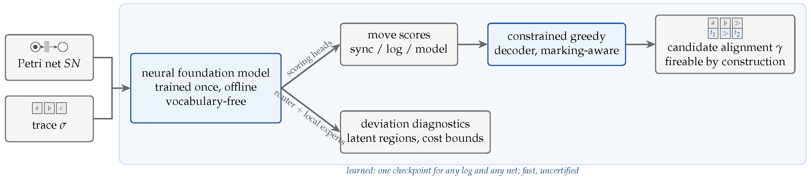
Figure 2.
The LARA architecture: coupled net and trace encoders feed the scoring heads; a constrained greedy decoder emits a fireable candidate that is verified by replay and certified or repaired by the exact backend.
Figure 2.
The LARA architecture: coupled net and trace encoders feed the scoring heads; a constrained greedy decoder emits a fireable candidate that is verified by replay and certified or repaired by the exact backend.
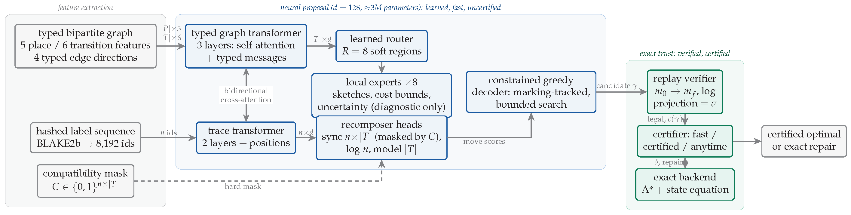
Figure 3.
The diagnostic decomposition branch on a small duplicate-label choice net, for a trace that skips event b: the learned router partitions the net into latent regions (three of shown), local experts predict deviation sketches and cost bounds, and the summed bounds estimate the alignment cost; all outputs are diagnostic only and never reach the decoder or exact search.
Figure 3.
The diagnostic decomposition branch on a small duplicate-label choice net, for a trace that skips event b: the learned router partitions the net into latent regions (three of shown), local experts predict deviation sketches and cost bounds, and the summed bounds estimate the alignment cost; all outputs are diagnostic only and never reach the decoder or exact search.
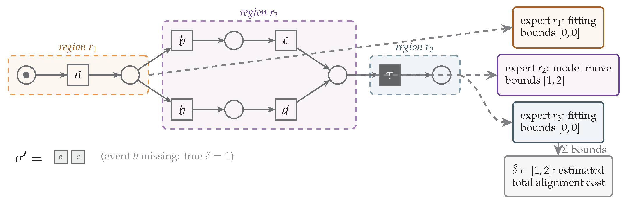
Figure 4.
Scoring and greedy decoding on the net of Figure 3 for the fitting trace : at event b two enabled transitions carry the label, so the synchronous scores, informed by the suffix through cross-attention, select ; the final bounded search reaches through the invisible transition. Every move fires on the tracked marking, so the candidate is fireable by construction.
Figure 4.
Scoring and greedy decoding on the net of Figure 3 for the fitting trace : at event b two enabled transitions carry the label, so the synchronous scores, informed by the suffix through cross-attention, select ; the final bounded search reaches through the invisible transition. Every move fires on the tracked marking, so the candidate is fireable by construction.
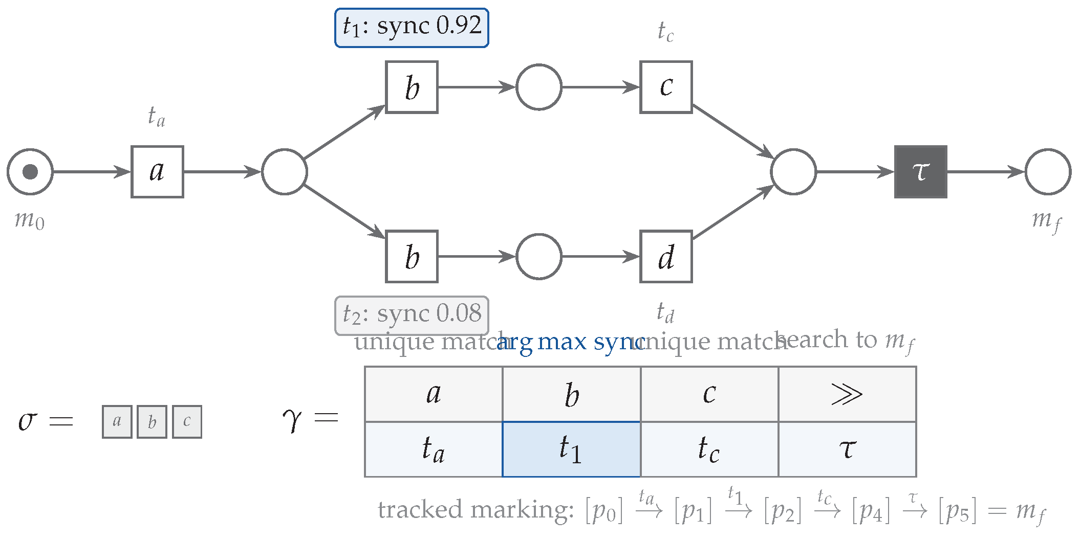
Figure 5.
Left: total loss per epoch of the reference run (dashed line: best validation epoch 18). Right: cost-gap distribution on the test split (); all non-zero gaps are even, the signature of greedy model-move detours.
Figure 5.
Left: total loss per epoch of the reference run (dashed line: best validation epoch 18). Right: cost-gap distribution on the test split (); all non-zero gaps are even, the signature of greedy model-move detours.

Figure 6.
Median alignment time per trace versus net size on block-structured nets (log-log). LARA stays at the forward-pass floor; exact A* degrades super-linearly, with first timeouts at size 40.
Figure 6.
Median alignment time per trace versus net size on block-structured nets (log-log). LARA stays at the forward-pass floor; exact A* degrades super-linearly, with first timeouts at size 40.
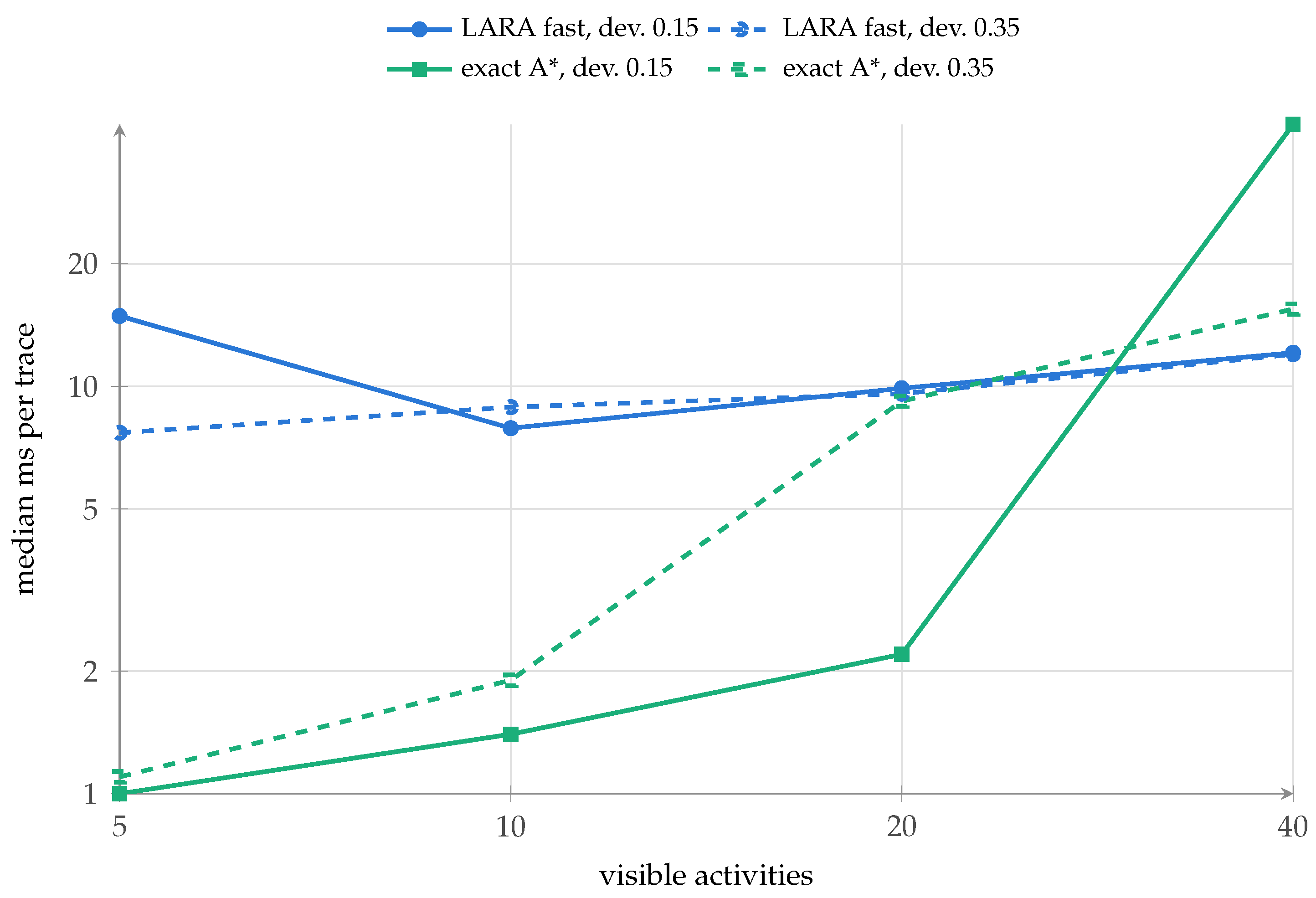

Table 1.
Headline results on the held-out test split ().
| metric | value |
|---|---|
| replayable (legal) alignments | 100.0% |
| equal to optimum cost | 88.0% |
| certified optimal (cost equality vs. exact) | 88.0% |
| exact transition-sequence match | 68.0% |
| label-level alignment match | 68.0% |
| mean / median cost gap | 0.38 / 0.00 |
| p90 / p95 / max cost gap | 2.0 / 4.0 / 6.0 |
Table 2.
Guidance ablation on the test split ().
| metric | unguided | guided | |
|---|---|---|---|
| replayable | 100.0% | 100.0% | 0.0 |
| equal to optimum cost | 83.0% | 88.0% | +5.0 |
| exact transition-sequence match | 63.0% | 68.0% | +5.0 |
| mean cost gap | 0.48 | 0.38 | −0.10 |
| sequence family, optimal () | 86.6% | 86.6% | 0.0 |
| duplicate-label family, optimal () | 66.7% | 94.4% | +27.7 |
| evaluation time (100 traces) | 1.0 s | 1.9 s | +0.9 s |
Table 3.
The learned cost estimate against the exact optimum on the held-out test split ().
| metric | value |
|---|---|
| mean absolute error of upper bounds vs. | 0.50 |
| mean signed error | −0.27 |
| Pearson correlation with | 0.89 |
| mean estimate on fitting traces () | 0.20 |
| mean estimate on deviating traces () | 1.73 |
| deviation detection accuracy (threshold 0.5) | 93.0% |
| mean interval width ( upper − lower) | 0.47 |
| interval coverage of | 22.0% |
Table 4.
Scaling benchmark on random block-structured nets (10 samples per configuration; exact timeout 30 s, timeouts counted at the timeout).
Table 4.
Scaling benchmark on random block-structured nets (10 samples per configuration; exact timeout 30 s, timeouts counted at the timeout).
| size | dev. | legal | optimal | mean gap | fast med. | exact med. | speedup | t/o | |
|---|---|---|---|---|---|---|---|---|---|
| 5 | 0.15 | 7 | 100% | 80% | 0.3 | 14.9 ms | 1.0 ms | 0.07× | 0 |
| 5 | 0.35 | 6 | 100% | 60% | 1.6 | 7.7 ms | 1.1 ms | 0.14× | 0 |
| 10 | 0.15 | 13 | 100% | 80% | 1.2 | 7.9 ms | 1.4 ms | 0.17× | 0 |
| 10 | 0.35 | 13 | 100% | 40% | 1.8 | 8.9 ms | 1.9 ms | 0.21× | 0 |
| 20 | 0.15 | 28 | 100% | 60% | 3.6 | 9.9 ms | 2.2 ms | 0.22× | 0 |
| 20 | 0.35 | 26 | 100% | 50% | 3.0 | 9.6 ms | 9.2 ms | 0.96× | 0 |
| 40 | 0.15 | 55 | 100% | 30% | 8.4 | 12.1 ms | 44.0 ms | 3.65× | 0 |
| 40 | 0.35 | 54 | 100% | 33% | 11.6 | 12.0 ms | 15.5 ms | 1.29× | 1 |
Table 5.
Zero-shot results on real-life logs with inductive-miner models (per variant; trace-wtd. weights variants by frequency).
Table 5.
Zero-shot results on real-life logs with inductive-miner models (per variant; trace-wtd. weights variants by frequency).
| log | noise | net ( / ) | legal | optimal | gap | median time | |
|---|---|---|---|---|---|---|---|
| variant | trace-wtd. | mean/max | LARA / exact | ||||
| road traffic | 0.0 | 15 / 10+10 | 100% | 100.0% | 100.0% | 0 / 0 | 8.0 / 1.7 ms |
| road traffic | 0.5 | 13 / 10+7 | 100% | 70.0% | 94.0% | 0.50 / 3 | 7.9 / 1.3 ms |
| receipt | 0.0 | 45 / 27+47 | 100% | 50.0% | 82.6% | 0.76 / 5 | 18.5 / 27.4 ms |
| receipt | 0.5 | 25 / 24+19 | 100% | 55.2% | 74.6% | 0.82 / 7 | 8.9 / 8.1 ms |
Disclaimer/Publisher’s Note: The statements, opinions and data contained in all publications are solely those of the individual author(s) and contributor(s) and not of MDPI and/or the editor(s). MDPI and/or the editor(s) disclaim responsibility for any injury to people or property resulting from any ideas, methods, instructions or products referred to in the content. |
© 2026 by the authors. Licensee MDPI, Basel, Switzerland. This article is an open access article distributed under the terms and conditions of the Creative Commons Attribution (CC BY) license (http://creativecommons.org/licenses/by/4.0/).
Copyright: This open access article is published under a Creative Commons CC BY 4.0 license, which permit the free download, distribution, and reuse, provided that the author and preprint are cited in any reuse.


