

Submitted:
06 July 2026
Posted:
08 July 2026
You are already at the latest version
Abstract
Alignment-based conformance checking is a central task in process mining, but computing optimal alignments is computationally hard. This paper studies whether the alignment problem can be expressed directly as a Quadratic Unconstrained Binary Optimization problem and explored with quantum annealing. We present a direct QUBO formulation for optimal alignments on safe Petri nets, with a proof-of-concept implementation supporting exact solving, simulated annealing, and a D-Wave Advantage2 quantum processing unit. The study is intentionally preliminary: rather than claiming a practical quantum advantage, we test whether the formulation is semantically correct and where current hardware helps or fails. On small representative benchmarks, the QUBO recovers correct optimal alignments, including concurrency, loops, silent transitions, and duplicate labels. On loop-heavy instances, the quantum annealer can outperform simulated annealing on success probability. Scalability, however, is strongly limited by hardware connectivity and embedding overhead. Overall, direct QUBO-based alignment finding is feasible in principle, but still far from practical large-scale use.
Keywords:
conformance checking
; alignments
; petri nets
; qubo
; quantum annealing
; feasibility study
1. Introduction
Process mining studies how event data can be used to analyze, monitor, and improve real processes (van der Aalst 2016). Within this area, conformance checking compares the behavior recorded in an event log with the behavior allowed by a process model (Carmona et al. 2022). One of the most informative techniques for this task is based on alignments, which explain a trace as a sequence of synchronous moves, log moves, and model moves (van der Aalst et al. 2012). Because log-level conformance is computed by solving this problem repeatedly for traces or trace variants, optimal alignment finding is a core computational task behind alignment-based conformance checking.
Optimal alignments, however, can be expensive to compute: for important classes of process models the problem is computationally hard, and the cost grows quickly with model size, trace length, and control-flow complexity (Schwanen et al. 2025). Alignment-based conformance checking can thus become costly exactly where it is most informative. Previous work on SAT and MILP encodings shows that alignment finding can be expressed in general optimization formalisms beyond classical shortest-path search (Boltenhagen et al. 2021,Chatain and Carmona 2016,Schwanen et al. 2024), so it is natural to ask whether the same problem can be encoded in a form compatible with quantum optimization.
In this paper, we study the alignment problem through the lens of Quadratic Unconstrained Binary Optimization, or QUBO (Punnen 2022). A QUBO represents an optimization problem over binary variables using linear and quadratic terms, and it can be handled by exact solvers, classical heuristics, and quantum annealers (Rajak et al. 2022), so one representation can be explored across different computational backends. Current hardware faces strong connectivity and embedding constraints, so quantum annealing is not yet ready for practical conformance checking, but a QUBO formulation lets us study in a controlled way whether alignment semantics can be translated faithfully into a quantum-compatible optimization problem.
Our focus is deliberately narrow: we neither study end-to-end log conformance on industrial event logs nor claim that quantum hardware already outperforms strong classical conformance checking algorithms. Instead, we present a direct QUBO formulation for optimal alignments on safe Petri nets, together with a proof-of-concept implementation that supports exact solving, classical simulated annealing, and execution on a D-Wave Advantage2 quantum processing unit (D-Wave Systems 2025a). The goal is to understand whether this formulation is semantically correct, when it appears promising, and what currently prevents it from scaling. The paper synthesizes and refines ideas first developed in a M.Sc. thesis (Geuskens 2026a).
This paper is therefore a preliminary study with a mixed but informative empirical picture. On small representative benchmarks, the QUBO recovers correct optimal alignments, including cases with concurrency, loops, silent transitions, and duplicate labels, while scalability is strongly limited by current hardware connectivity and the overhead of minor embedding. Between these two results, one interesting signal emerges: on some loop-heavy instances, the quantum annealer performs better than classical simulated annealing on the same logical QUBO. Figure 1 summarizes the logic of the paper.
To be meaningful for process mining, this line of work must clarify whether the direct QUBO computes the same optimal alignments as standard conformance checking, which properties of models and traces make the encoding easy or hard, whether quantum annealing helps on at least some instance classes, and whether current hardware can represent the formulation robustly, leading to the following research questions:
- RQ1.
- Can standard optimal alignment finding be expressed directly as a QUBO and solved correctly on small representative Petri net examples?
- RQ2.
- Which properties of a process model or trace make the resulting QUBO easy or hard to solve?
- RQ3.
- Are there classes of alignment instances for which a quantum annealer performs better than classical simulated annealing on the same QUBO?
- RQ4.
- What currently prevents this approach from scaling to more realistic conformance checking tasks?
The paper makes three contributions: a direct QUBO formulation for optimal alignments on safe Petri nets, a proof-of-concept implementation with an empirical evaluation on exact, classical, and quantum backends, and process mining insights about correctness, difficulty, promising cases, and present scalability limits.
2. Related Work
Related research falls into three lines of work: classical alignment computation, alternative optimization encodings for alignment problems, and QUBO or quantum-optimization methods.
2.1. Classical Alignment Computation in Process Mining
Alignments were introduced as a cost-based way to compare observed behavior in an event log with the behavior allowed by a process model (van der Aalst et al. 2012). In the classical process mining literature, the standard exact approach is based on synchronous product nets, which combine the process model and the trace into one search structure (Adriansyah et al. 2011). Optimal alignments can then be computed by shortest-path or heuristic-search techniques, most notably -based methods (Carmona et al. 2022,van Dongen 2018).
These methods remain the main reference point because they compute standard optimal alignments with strong correctness guarantees (Carmona et al. 2022). However, the problem remains computationally hard (Schwanen et al. 2025), which motivates alternative formulations. Our work does not replace this classical view; it asks whether the same optimization target can be expressed in a different computational language, namely QUBO.
2.2. Alternative Optimization Encodings for Alignment Problems
A second line of work studies alignment and conformance checking problems through general optimization or satisfiability formalisms rather than explicit state-space search. SAT-based encodings have shown that alignment-related conformance tasks can be represented by bounded logical constraints (Boltenhagen et al. 2021,Chatain and Carmona 2016). Likewise, mixed-integer linear optimization has been used to formulate alignment computation for specific model classes such as process trees (Schwanen et al. 2024).
These works are close in spirit to ours because they move alignment reasoning into a generic optimization formalism, but they neither provide a direct QUBO formulation of standard optimal alignments on safe Petri nets nor design their encodings with quantum annealing in mind. In contrast, we construct the alignment problem directly in a quadratic binary form that can be executed by exact solvers, classical QUBO samplers, and a quantum annealer without changing the logical problem definition.
2.3. QUBO and Quantum Optimization
QUBO is a standard modeling formalism for combinatorial optimization over binary variables (Punnen 2022). It is relevant here because the same formulation can be handled by classical heuristics and by quantum annealing (Rajak et al. 2022). In the broader optimization literature, generic reductions from SAT to QUBO (Nülein et al. 2023,Zielinski et al. 2023) and from integer linear programs to quantum-optimization settings (Chang et al. 2020) show that many discrete optimization problems can, in principle, be translated into a quantum-compatible form.
This line of work is enabling rather than process mining-specific: since SAT and MILP encodings of alignments already exist, indirect translations to QUBO are possible in principle, but such routes introduce many auxiliary variables, do not exploit the semantics of the original problem, and are unlikely to be the most compact or process-aware way to represent Petri net behavior on current quantum hardware. This is the main reason for pursuing a direct encoding instead of a pipeline such as alignment → SAT → QUBO.
Overall, to the best of our knowledge, prior work neither provides a direct QUBO formulation of standard optimal alignments for safe Petri nets, nor studies such a formulation from a process mining perspective using exact, classical stochastic, and quantum execution backends; this is the gap addressed here.
3. Preliminaries
3.1. Traces and Safe Petri Nets
A trace records one observed execution of a process as a finite sequence of activity labels (van der Aalst 2016). We write a trace as , where each belongs to an activity alphabet . In this paper, we solve the alignment problem for one trace at a time.
We use labeled safe Petri nets as process models (Desel et al. 2004,van der Aalst 2016). A Petri net is a tuple , where P is a set of places, T is a set of transitions with , is the flow relation, and is a labeling function. A transition labeled is silent, meaning that it has no corresponding event in the trace. Different transitions may share the same visible label.
A marking assigns tokens to places. Because we restrict ourselves to safe Petri nets, every place contains at most one token, so a marking can be seen as a function . For a transition , we write and for its input and output places. Similarly, for a place , we write and .
A transition t is enabled in marking M if each input place of t contains a token, that is, if for all . Firing an enabled transition produces a new marking given by
Given an initial marking and a final marking , a firing sequence is called a model run if it transforms into .
3.2. Alignments
Alignment-based conformance checking compares a trace and a process model by means of a sequence of moves (van der Aalst et al. 2012). Each move has a trace side and a model side. We use the placeholder symbol − to denote the absence of an activity or transition. A synchronous move has the form with . A log move has the form , meaning that the trace advances without firing a model transition. A model move has the form , meaning that the model fires a transition without consuming a trace event.
An alignment of trace to model N is a sequence of such moves whose first components, after removing all occurrences of −, reproduce exactly , while the second components, after removing all occurrences of −, form a model run of N. We denote the set of all alignments of to N by .
We use the standard alignment cost: synchronous moves have cost 0, log moves and visible model moves have cost 1, and model moves on silent transitions have cost 0 (Carmona et al. 2022,van der Aalst et al. 2012). Formally, for a move m,
The cost of an alignment is . An optimal alignment is an alignment with minimum total cost. We write for the cost of an optimal alignment.
3.3. Quadratic Unconstrained Binary Optimization
A QUBO problem is an optimization problem over binary variables (Punnen 2022). In its standard form,
where is a binary vector, Q contains quadratic interaction terms, and contains linear terms. The function H is often called the energy of the QUBO.
Because a QUBO is unconstrained, logical or combinatorial constraints are usually enforced through penalty terms. A common construction is
where represents the optimization objective, penalizes invalid solutions, and is a penalty factor. The goal is to choose large enough so that invalid solutions never become more attractive than valid ones.
3.4. Quantum Annealing and Embeddings
Quantum annealing is a hardware-based method for searching for low-energy solutions of a QUBO (Rajak et al. 2022). Unlike an exact solver, a quantum annealer does not guarantee that the optimum is found; it returns a collection of candidate solutions, usually called samples, and the lowest-energy samples are taken as the most promising ones.
On real hardware, the logical QUBO cannot always be mapped directly to the physical processor because not every pair of physical qubits is connected (D-Wave Systems 2026). Therefore, a minor embedding is required: one logical variable may need to be represented by a chain of physical qubits. Long or highly connected chains are more fragile, and chain breaks can reduce solution quality; in the evaluation, this is one of the main bottlenecks for scalability.
4. Approach
4.1. Problem Setting and High-Level Idea
Let be a trace, let be a safe labeled Petri net, and let and be its initial and final markings. We assume first that and discuss the empty trace at the end of this section. Let be a fixed alignment horizon with .
The goal is to encode the problem of finding an optimal alignment of to N as one QUBO. Since a QUBO has a fixed number of variables, we encode exactly Sslots instead of a variable-length alignment. Each slot may represent one of four possibilities: a synchronous move , where one trace event is consumed and one transition with the same visible label is fired; a log move , where one trace event is consumed and no transition is fired; a model move , where one transition is fired and no trace event is consumed; or a filler move , where neither the trace nor the model advances. Filler moves have zero cost and are removed after decoding; they are needed because the optimal alignment may be shorter than S. A zero-constraint-energy assignment should describe a padded alignment that satisfies three requirements: the trace events are consumed exactly once and in the correct order; the model-side transition sequence is a valid Petri net run from to ; and every slot that consumes a trace event and fires a transition is label-consistent. Among all such valid padded alignments, the QUBO objective minimizes the standard alignment cost.
Figure 2 introduces the running example used in this section, and Figure 3 shows the fixed-length view of the encoding.
We use the Iverson bracket notation , which evaluates to 1 if statement is true and to 0 otherwise.
At a high level, each slot stores the state before the slot (the current marking of the Petri net and the current position in the trace) and the action in the slot (whether one trace event is consumed and which model transition, if any, is fired). The constraints ensure that the state before slot is exactly the result of applying the action in slot s to the state before slot s.
4.2. Decision Variables
For every slot , transition , and trace position , we introduce the following binary variables:
- : equals 1 if transition t is fired in slot s.
- : equals 1 if slot s consumes one trace event.
- : equals 1 if, before slot s, the next unconsumed trace event is . The state means that the complete trace has already been consumed.
- : auxiliary variable intended to represent .
- for : auxiliary variable intended to represent , that is, slot s consumes event .
For every place and , we introduce marking variables . The variable describes the marking before slot s, and describes the marking after the final slot. The initial and final markings are fixed: and for all . Likewise, the trace starts at its first event: and for all . In the implementation, these fixed variables are substituted by constants and removed from the QUBO.
The auxiliary variables are purely technical: without them, the natural label-consistency and trace-update constraints would contain cubic terms; and keep the formulation quadratic.
4.3. Constraint Terms
We now define the constraint part of the QUBO. Each term is nonnegative and equals zero exactly when the corresponding rule is respected, possibly together with the auxiliary-variable constraints on which it depends; the full constraint energy, the sum of all terms, is therefore zero if and only if every individual constraint is satisfied.
One trace position per slot. Before each slot, the encoding must point to exactly one trace position:
At most one transition per slot. A single alignment slot may fire at most one model transition. Let . The condition is enforced by
For binary variables this term is zero if no transition or exactly one transition is selected, and positive otherwise.
Trace-event consumption. If slot s consumes a trace event, then it must consume exactly the current trace event. The variables identify which event is consumed. We enforce and . The corresponding QUBO penalties are
and
Together with the one-hot constraint on , these terms imply that is possible only when the trace pointer is at some real event position , and then exactly the current event is consumed; if the pointer is already at , then is forced.
Trace-index update. The trace pointer should advance by one exactly when an event is consumed. For convenience, define . Then the trace-index update is for and . This is enforced by
The sum stops at because is defined only before the S slots. Completion of the trace at the end of slot S is handled separately below.
Auxiliary product for synchronous moves. A slot is synchronous precisely when it both consumes a trace event and fires a transition. To keep label-consistency quadratic, we introduce and enforce it with the standard quadratic reduction
For binary variables, the summand is zero exactly when .
Label-consistent synchronous moves. Together with , label consistency is enforced by
If and , then , and since for exactly one current trace position, the term above is zero only if the fired transition has the same visible label as the current trace event. In particular, a silent transition cannot be used as a synchronous move, because is not a trace activity label.
Petri net state update. The marking must evolve according to the Petri net firing rule: we require for every place p. This is enforced by
This equation also enforces ordinary enabling conditions: if a transition consumes a token without reproducing it, the equation cannot be satisfied unless the token is present before the slot, and because markings are binary, it prevents producing a token into an already marked place.
A small extra term is needed only for self-loop arcs, where a transition both consumes from and produces to the same place. There, the consume and produce effects cancel in the marking equation, so the equation alone does not check whether the token was present before firing. Let . Then
ensures that such a transition can fire only if the self-loop place is marked.
Complete trace consumption. By the end of the horizon, the full trace must have been consumed. Since means that the trace has already been consumed before slot S, and means that the final event is consumed in slot S, trace completion is expressed by the OR condition . The corresponding quadratic penalty is
Putting everything together, the full constraint energy is
Empty trace. For , the trace is already consumed at the start. One may then either omit the trace-index variables entirely or keep a single fixed state for all slots. There are no y variables, is omitted, and reduces to , which forces for all slots. The remaining marking and transition constraints are unchanged, so the QUBO searches for a model run from to using only model moves and filler moves.
4.4. Objective Function and Decoding
Among all feasible encodings, we minimize the standard alignment cost. A log move occurs when a trace event is consumed but no transition is fired. A visible model move occurs when a visible transition is fired but no trace event is consumed. Therefore, the objective is
On every feasible encoding, each slot has at most one fired transition, so counts exactly the log moves and visible model moves and thus equals the standard alignment cost.
The final QUBO is
where is a penalty factor.
Decoding a feasible binary solution is immediate. For each slot s: if and exactly one , the slot becomes the synchronous move where ; if and all , it becomes the log move where ; if and exactly one , it becomes the model move ; and if and all , it is a filler move and is removed. A zero-constraint-energy assignment cannot have any other slot type.
4.5. Search-Space Reduction
Before constructing the final QUBO, several variables can be fixed without changing the set of valid alignments.
First, before slot s, at most trace events can have been consumed, so the next trace position cannot be larger than s. Hence, for all , the variables can be fixed to 0, and consequently as well.
Second, the Petri net can rule out some states and actions early in the horizon. We compute conservative earliest-reachability lower bounds for places and transitions: if a place cannot possibly be marked before slot s, then is fixed to 0, and if a transition cannot possibly be enabled in slot s, then is fixed to 0. A variable is fixed only when the corresponding state or action is impossible in every valid run, so the pruning is safe.
These reductions preserve correctness while shrinking the QUBO and easing its embedding onto quantum hardware.
4.6. Correctness of the Encoding
We now state the correctness guarantee. Because the horizon is fixed, the result is necessarily relative to the set of alignments whose length is at most S. Let be the set of valid alignments of to N with length at most S.
Proposition 1.
Let σ be a trace with , let N be a safe labeled Petri net with initial marking and final marking , and let . Assume that . Consider the QUBO defined above, with the fixed initial and final marking variables and the fixed initial trace-index variables substituted into the QUBO. If , then:
- 1.
- every alignment can be represented by a binary assignment with and ;
- 2.
- every global minimizer of satisfies and decodes to an optimal alignment in .
Proof.
We prove the claim in four steps.
Step 1: zero-constraint energy implies a valid padded alignment. Let be a binary assignment with . Since is a sum of nonnegative terms, every individual constraint term must be zero.
From , each slot s has exactly one active trace-index variable . From , at most one transition is selected in each slot.
The terms and imply that if and only if exactly one is active, and any active must correspond to the current trace position . Thus, when a slot consumes a trace event, it consumes the current one. If the pointer is already at , then for all , forcing all and hence : no event can be consumed after the trace has been completed.
The term enforces for every . Hence the trace pointer advances by exactly one when an event is consumed and otherwise stays unchanged. Since the initial trace position is fixed to , the consumed trace events are exactly a prefix of and are consumed in order. Finally, implies or : either the full trace has been consumed before slot S, or the final trace event is consumed in slot S. Consequently, the trace projection of the decoded non-filler slots is exactly .
Next consider the model side. The initial marking is fixed to , and the final marking after slot S is fixed to . Since , every slot satisfies for all . If no transition is fired in slot s, this equation leaves every place unchanged. If a transition t is fired, the equation applies exactly the Petri net token update. For every input place , it requires , possible with binary variables only if , so the consumed token must be present. For every output place , it requires , possible only if , so the update remains safe. For self-loop places , the effects cancel in the marking equation, and enforces whenever . Therefore every fired transition is enabled and the marking update is valid. Since , the model-side projection is a model run from to .
It remains to check synchronous moves. From , each equals . If a slot both consumes an event and fires transition t, then , and since exactly one trace-index variable is active, implies for the active trace event . Hence every slot that is both a trace move and a model move is a legal synchronous move. Thus every assignment with decodes to a valid alignment padded with filler moves.
Step 2: every bounded valid alignment has a zero-constraint encoding. Let be any valid alignment with length , padded with filler moves to exactly S slots.
We assign the variables slot by slot. Before each slot s, set to the marking reached by the model projection of the previous non-filler slots, and set for the next unconsumed trace position j. For a log move, set and all ; for a model move , and ; for a synchronous move , and ; for a filler move, and all . In all cases, set and . The next marking and next trace index are then set according to the actual alignment move.
Because is a valid alignment, its trace projection is exactly , its model projection is a valid run from to , and every synchronous move has a matching label. Therefore all trace-index, marking, self-loop, auxiliary-product, label-consistency, and completion constraints are satisfied, and the resulting binary assignment has .
Step 3: for feasible assignments, the objective equals alignment cost. Let satisfy . Then each slot has at most one selected transition. If and no transition is selected (log move), the first part of (12) contributes 1 and the second 0. If and one transition is selected (synchronous move), the first part contributes 0 and the second is multiplied by . If and one visible transition is selected (visible model move), the first part contributes 0 and the second 1. If and one silent transition is selected (silent model move), or no transition is selected (filler move), both parts contribute 0. Thus counts exactly the log moves and visible model moves, and therefore equals the standard alignment cost of the decoded alignment.
Step 4: global minimizers are feasible and optimal. Since , by Step 2 there exists a feasible assignment, and by Step 3 every feasible assignment has objective value at most S, because each slot contributes at most one unit of alignment cost.
It remains to show that no infeasible assignment can have lower total energy when . All constraint terms are nonnegative integer-valued on binary assignments, so any violated constraint gives positive constraint energy. The only subtlety is that can be negative on infeasible assignments if more than one transition is selected in a slot while ; this is penalized by .
For a slot s, write . The slot contribution of is , and that of is . If , this objective contribution is nonnegative. If , it equals , which is again nonnegative for . For , the combined objective-plus-transition-penalty contribution is , which is positive and at least . Since , this is larger than S.
Therefore an infeasible assignment either violates some constraint other than , in which case its total energy is at least after accounting for the nonnegative combined contribution of , or it violates only , in which case the previous paragraph shows that its total energy already exceeds S. In both cases its energy is greater than S.
Since some feasible assignment has energy at most S, every global minimizer has . Among feasible assignments, , which by Step 3 equals the alignment cost. Therefore every global minimizer decodes to an alignment of minimum cost in . □
Proposition 1 shows that the proposed QUBO solves the standard alignment problem up to the chosen horizon S. If is empty, then no feasible zero-constraint assignment exists; in that case, the horizon is too small and must be increased.
5. Implementation
5.1. Overall Workflow
Given a trace , a safe Petri net N, and a horizon S, the implementation performs four steps:
This separation matters for the evaluation: the encoder always produces the same logical optimization problem, while the execution backend can be exchanged, so all backends can be compared on the same QUBO instance.
The implementation is available as the intentionally lightweight Python package qps (Geuskens 2026b), which focuses on constructing, executing, and decoding the alignment QUBO rather than on providing a full process mining framework.
5.2. QUBO Construction and Variable Fixing
The encoder constructs the objective term , the constraint term , and the combined QUBO exactly as described in Section 4. The parts are kept separate because, after solving or sampling, we also want to know whether a returned assignment is feasible and, if so, what alignment cost it represents2.
Before execution, the implementation applies the safe variable-fixing reductions described in subsec:approachpruning: trace-based pruning of impossible trace-index and consumption variables, and model-based pruning using earliest-reachability bounds for places and transitions. The reductions only shrink the logical QUBO before it reaches the selected backend; the model-based bounds are computed once per Petri net and reused across its traces.
The remaining QUBO is smaller and usually easier to solve or embed, which is especially important for quantum execution, where every unnecessary logical variable may lead to additional physical qubits and longer chains.
5.3. Execution Backends
The reduced QUBO can be executed with different backends.
For exact reference solutions, the implementation linearizes the quadratic terms and solves the result with SCIP (Hojny et al. 2025). These solutions verify that the lowest-energy feasible assignments indeed correspond to optimal alignments.
As a classical stochastic baseline, the same logical QUBO is sampled with simulated annealing, which samples low-energy states through iterative Metropolis-Hastings updates while gradually lowering an effective temperature. This baseline is not a simulation of the quantum hardware, so the classical sampler and the quantum annealer can be compared without changing the alignment encoding.
For quantum execution, the implementation uses D-Wave’s Ocean toolchain (D-Wave Systems 2025b,D-Wave Systems 2025c). The encoder still produces only the logical QUBO; hardware-specific steps such as coefficient scaling, minor embedding, chain-strength selection, sampling on the QPU, and unembedding of the returned samples are handled by the D-Wave software stack. The encoder thus defines what optimization problem should be solved, whereas the selected backend determines how it is executed3.
5.4. Feasibility Checking and Decoding
After solving or sampling, each returned binary assignment is evaluated on and separately, and only assignments with are treated as feasible. This filtering is essential for stochastic methods, because low total energy does not imply that an assignment is a valid alignment4.
Feasible assignments are then decoded slot by slot from left to right: using the variables and , the decoder reconstructs whether slot s represents a synchronous, log, model, or filler move, and filler moves are removed. If only the alignment cost is needed, full decoding is unnecessary, since on feasible assignments already equals the standard alignment cost; this is useful for fitness computation over many traces.
5.5. Reuse Across Traces
In process mining, many traces or trace variants must usually be aligned against the same process model. The implementation therefore reuses all model-dependent preprocessing across traces, most notably the earliest-reachability bounds introduced above. Moreover, traces of the same length share the same general variable layout, so only trace-specific label-dependent terms need updating. This does not remove the cost of solving the optimization problem itself, but it reduces repeated preprocessing in larger experiment batches.
The prototype prioritizes transparency and faithfulness to the mathematical formulation over aggressive low-level optimization, which is appropriate for studying the encoding itself across backends.
6. Evaluation
The evaluation addresses four questions: whether the proposed QUBO recovers correct optimal alignments, which factors drive instance difficulty, when the QPU helps compared with simulated annealing, and what currently limits scalability5.
6.1. Experimental Setup
The evaluation is designed as a controlled proof-of-concept study.
Benchmark models and traces. We use handcrafted safe Petri nets that isolate the control-flow patterns most relevant to alignment computation: sequential nets , exclusive-choice nets , parallel nets , loop nets , and flower models . In addition, we use a slightly richer toy model for parameter studies, one variant with a silent transition, and one variant with duplicate visible labels. For each model, we manually construct both fitting and non-fitting traces covering simple deviations such as missing events, extra events, wrong routing choices, and repeated loop behavior6.
These benchmark instances are intentionally small: with current hardware, realistic mined Petri nets and real-life event logs would typically yield QUBOs too large or too densely connected for a clean study of the method. The synthetic setting separates two issues that would otherwise be mixed: whether the encoding is correct, and whether current hardware can handle it.
Execution backends.Table 1 summarizes the tools used in the evaluation7. Unless an experiment explicitly studies a parameter, backend settings are kept at their defaults, which avoids tuning one backend more aggressively than another.
The QPU is accessed through D-Wave’s Ocean SDK (D-Wave Systems 2025b,D-Wave Systems 2025c), exact solutions are obtained by linearizing the QUBO and solving it with SCIP (Hojny et al. 2025), and simulated annealing serves as the main classical baseline because it solves the same logical QUBO without changing the problem formulation. Classical preprocessing and baseline runs are executed on an HPC system with Intel Xeon Sapphire CPUs.
Correctness reference. For every benchmark instance, we compute an exact optimum with SCIP and compare its cost with the cost returned by a standard process mining alignment implementation in PM4Py. The two references agree on all instances, so the true optimum is known and we can evaluate whether a sample is not only feasible but also globally optimal.
Reported metrics. We report two groups of metrics. The first concerns alignment quality: the feasibility rate (fraction of returned samples with ), the success probability (fraction of samples achieving the known global optimum), the recall (fraction of distinct optimal alignments appearing in the sample set), and, when useful, the 95% samples-to-solution, which summarizes how many samples are needed to observe an optimal solution with high probability.
The second group concerns QUBO and hardware complexity: the number of logical QUBO variables and, for QPU runs, the number of physical qubits after embedding, the number and length of chains, the mean chain-break fraction, and the QPU access time. Unless stated otherwise, QPU timing refers to the access time reported by the backend and excludes internet and cloud-queue latency, which depends on the client connection rather than the alignment encoding.
Experiment-specific parameters. The alignment horizon S, the penalty factor , the QPU annealing time, and the chain strength are part of the phenomenon under study, so each experiment states which values are used and, when relevant, varied. This is especially important for S, which directly controls the size of the QUBO and thus strongly influences both classical and quantum performance.
Finally, because minor embedding on the QPU is heuristic, different embeddings of the same logical QUBO can lead to slightly different results. Where this variation matters, we repeat QPU runs and report averages, stating the number of repetitions.
6.2. Can the Method Recover Correct Optimal Alignments?
Test cases. We use the benchmark families introduced above (, , , , ) plus two correctness-sensitive variants: one model with a silent transition and one with duplicate visible labels. Together, these benchmarks cover the main sources of difficulty for alignment semantics: sequential replay, routing choices, multiple optimal alignments caused by concurrency, repeated loop behavior, silent model behavior, and ambiguity caused by non-unique visible labels.
Because the instances can be inspected manually, the distinct optimal alignments were known, so recall can be computed exactly.
Main result. Across all basic benchmark families, the proposed QUBO recovers the correct optimal alignments: the exact solver, simulated annealing, and the QPU agree on the optimum alignment cost, and both samplers achieve recall 1.
This is the central correctness result of the paper: the encoding is not merely producing plausible low-energy solutions, since the lowest feasible QUBO solutions correspond exactly to standard optimal alignments8.
Table 2 highlights that the result is not limited to fitting sequential traces: the encoding also behaves correctly for concurrency, silent transitions, and duplicate visible labels, which often cause trouble in conformance checking.
Why these cases matter. In parallel models, several explanations of the same trace can be equally good, and a correct alignment method should not artificially prefer one execution order. Silent transitions are common in discovered and manually designed models, so an encoding that cannot represent silent model moves would be of limited use. Duplicate labels occur when different states of a process share the same visible activity name; correctness then requires reasoning at the transition level. Figure 4 illustrates these three cases.
Recall of all optimal alignments. Because the basic instances are small, we can also ask whether the samplers return all distinct optimal alignments, which is especially relevant for parallel models. Figure 5 summarizes the recall: for every family, both the QPU and simulated annealing achieve recall 1, so on these small cases the stochastic nature of the samplers is not a correctness problem.
Interpretation. For the representative small cases studied here, the method produces the right answer, including the semantic corner cases that matter in practice. The results show something modest but fundamental: the direct QUBO formulation is semantically faithful to standard alignment computation on these benchmark classes.
6.3. What Makes Instances Easy or Hard?
We now ask which properties of an instance make the resulting QUBO easy or hard to solve; for process mining users, this tells us when the method is likely to work well and why it may fail. We study three factors: the alignment horizon S, the structure of the Petri net, and the trace length.
The horizon S is the strongest difficulty driver. The horizon S fixes the maximum number of slots the QUBO may use. If S is larger than the true optimal alignment length, the optimal alignment does not change; the QUBO simply gets extra room for filler moves. The effect of S is therefore easy to interpret: any degradation as S increases comes from the larger search space and the harder embedding, not from a change in alignment semantics.
This is exactly what we observe. As S grows, the number of logical QUBO variables grows linearly, but the number of required physical qubits grows faster, because the larger logical problem induces more chains and more interactions between them. Feasibility and success probability drop, especially on the QPU; simulated annealing also weakens, but more gradually.
For a practitioner, the takeaway is that S should be chosen as tightly as possible: too small may exclude the true optimum, while too large makes the QUBO harder for both samplers, and especially for the QPU.
Model structure matters, not only model size. A second important result is that two models of similar size can behave very differently: exclusive-choice models become difficult much faster than certain similarly sized parallel models, even when the latter use at least as many logical variables. The main issue is how interactions are distributed inside the QUBO.
Choice-heavy models create a few variables that interact with many others; when such highly connected variables are embedded on the QPU, the corresponding chains are pulled by many neighboring couplings at once, which increases the chance of chain breaks. In contrast, a more distributed structure can be easier for the hardware even with slightly more variables overall. Figure 7 visualizes this contrast between a hub-like interaction pattern and a more distributed one.
Trace length is also a difficulty factor, but less cleanly. Longer traces produce larger QUBOs because the trace-index part of the encoding grows. However, unlike the horizon S, trace length also changes the alignment problem itself: there are more events to explain and more positions at which deviations can occur, so its effect is less regular than that of S. In particular, on loop-based models, longer traces can create many competing near-optimal explanations, changing both the size and the shape of the search landscape. We return to this in Section 6.4, where loop-heavy cases turn out to be the most promising ones for the QPU.
Summary of the difficulty results.Table 3 summarizes the main insights of this subsection for a process mining reader.
Together, these results answer RQ2: the hardest instances are not merely the biggest ones. The most important difficulty drivers are a loose horizon S and a model structure that concentrates many interactions on a few variables; difficulty depends on how the process is structured, not only on how large it is.
6.4. When Does the QPU Help?
We now compare the QPU with simulated annealing (SA) on the same logical QUBO. The question is not whether the QPU is better in general, which would be too strong a claim on current hardware, but whether there are specific alignment instances for which the QPU produces better solutions than a classical QUBO sampler.
Overall comparison. Across the easier benchmark instances, both backends perform well, so these instances are too simple to reveal a meaningful advantage for either side. On the harder instances created by increasing the horizon S or by using embedding-unfriendly model structures, the QPU often degrades faster than SA because minor embedding and chain breaks become dominant. The evaluation therefore does not support a general claim that the QPU is better than SA for alignment finding, but the experiments reveal one clear exception: loop-heavy cases.
The main positive signal appears on loop-heavy instances. To study this effect, we keep the process model fixed as and increase the trace length10. The resulting instances remain interpretable, but become harder because the loop creates many competing explanations of the same observed behavior. Here the QPU achieves a higher success probability than SA for the longer traces, an effect not visible in the earlier benchmark families.
Figure 8 is the key result of this subsection: on the loop-based scaling experiment, the QPU overtakes SA on success probability. This is the strongest empirical reason to believe that quantum annealing may become useful for some process mining problems.
Why loops are different. In loop-heavy models, many alignments are close to correct but not quite optimal: early wrong choices in explaining a repeated fragment may still lead to a nearly optimal alignment later, creating a search space with many local minima. SA improves a solution through local updates, which can struggle when many low- and medium-quality explanations sit in separate valleys, whereas quantum annealing samples low-energy states of the full QUBO and may navigate such rugged landscapes more effectively. Figure 9 illustrates this. The explanation in terms of rugged landscapes and tunneling is consistent with the observed pattern, but remains an interpretation, not a proven mechanism.
Why the QPU doesnothelp everywhere. The QPU only helps when the logical search problem is hard but the physical embedding is still manageable. If the embedding becomes too fragile, chain breaks dominate and the potential benefit disappears, as in the larger or more densely connected instances discussed earlier. The loop-based advantage is therefore conditional: the search landscape must be hard enough to expose a weakness of SA, and the embedding must still be good enough that the QPU can represent the problem faithfully. Table 4 summarizes this subsection.
Takeaway for RQ3. The answer to RQ3 is mixed but positive in one specific sense: the evaluation does not show a broad advantage of the QPU over simulated annealing, but loop-heavy alignment instances are a promising case in which the QPU can produce better solutions than SA.
6.5. What Blocks Scalability Today?
The short answer to RQ4 is that the main scalability bottleneck is current hardware connectivity, not the alignment idea itself: the QUBO formulation remains logically correct as instances grow, but mapping it onto today’s quantum hardware becomes increasingly difficult.
The core problem is the logical-to-physical mapping. The alignment formulation lives on a logical level of binary variables and quadratic interactions, while the QPU operates on a physical graph of qubits and couplers that is not fully connected, so one logical variable often must be represented by a chain of several physical qubits. As already suggested by Figure 6, the number of logical variables grows only moderately with the horizon S, but the number of physical qubits can grow much faster: the QPU must solve an even larger embedded problem. Figure 10 illustrates this issue.
Chain breaks directly reduce alignment quality. Longer and more stressed chains are more likely to break, and a broken chain can turn an otherwise low-energy sample into an infeasible or suboptimal alignment. As chains become more numerous and fragile, the feasibility rate and success probability fall. This is exactly the pattern observed both when S increases and when model structure creates a few highly connected variables; the quality drop stems not from a change in alignment semantics, but from the physical difficulty of representing the logical interactions on hardware.
Topology matters more than raw qubit count. A particularly important result is that the limitation is not mainly the number of available qubits but how they are connected. Our experiments comparing increasing models with modified models make this point clearly11.
QPU performance drops quickly as n increases for , while for modified the number of logical variables is similar or even larger, yet the QPU remains much more stable. The instances concentrate many interactions on a few variables, which stresses the corresponding chains, while the modified instances distribute interactions more evenly, leading to fewer chain breaks at similar scale. Figure 11 visualizes this comparison and supports the strongest empirical statement of this subsection: connectivity and interaction distribution matter more than raw problem size alone.
A second practical limit is the need to choose S in advance. Even apart from hardware topology, the formulation requires a fixed horizon S: too small a horizon may exclude the optimal alignment entirely, while too large a horizon inflates the logical QUBO and the physical embedding, as seen in Section 6.3. The method therefore works best when a good upper bound on the alignment length is known, which realistic conformance checking cannot always guarantee.
What this means for process mining users. The limitation is not that the alignment problem is poorly expressed as a QUBO, since Section 6.2 showed that the encoding is semantically faithful; it is that today’s QPU hardware cannot yet represent larger or more interaction-heavy alignment QUBOs robustly enough. Table 5 summarizes the bottlenecks discussed above.
Answer to RQ4. What currently stops the approach from scaling is mainly the topology of the QPU: limited connectivity forces embeddings with many fragile chains, which break more often as the logical problem becomes larger or more unevenly connected.
6.6. Threats to Validity
The evaluation is intentionally narrow: it tests whether the proposed QUBO formulation is semantically correct, identifies the main difficulty drivers, and examines current hardware bottlenecks. This creates several limitations.
Small synthetic benchmarks. The experiments use small handcrafted Petri nets and traces rather than large real-life event logs. This isolates basic control-flow patterns and keeps the exact optimum verifiable, but it limits external validity: real mined models are often larger, noisier, and structurally less clean. The results are evidence for feasibility under controlled conditions, not of practical readiness on industrial-scale tasks.
Restriction to safe Petri nets and the standard cost model. The formulation targets safe labeled Petri nets and the standard alignment cost; these assumptions are reasonable for a first study, but richer cost models, broader net classes, and more specialized settings need additional work.
Dependence on the horizon S. In several correctness-oriented experiments, S is chosen close to the known optimum length so that the behavior of the encoding can be studied cleanly. In practice this length is not known in advance, so part of the evaluation is more favorable than a realistic deployment. Section 6.3 addresses this by varying S, but selecting a good horizon remains a real limitation.
Hardware-specific conclusions. The QPU results were obtained on one D-Wave Advantage2 system with the software stack and embedding tools available during the study, so the numerical breakpoints should not be over-generalized to future hardware or software. The stable conclusion is qualitative: embedding and connectivity constraints, not the logical QUBO, are the main scalability bottleneck.
Heuristic embeddings and stochastic variation. Minor embedding is heuristic, and both samplers are stochastic, so two executions of the same logical instance need not return the same solution distribution. We repeat QPU runs and report averages where embedding variation matters most, but some residual variability remains, one reason why the paper emphasizes robust qualitative patterns rather than isolated absolute numbers.
Comparison scope. The empirical comparison applies exact solving, simulated annealing, and quantum annealing to the same QUBO. This is the right comparison for evaluating the formulation itself, but not a benchmark against the strongest classical alignment algorithms, so the paper does not claim end-to-end superiority over state-of-the-art classical conformance checking.
Timing interpretation. For the QPU, cloud access and network latency are partly outside the control of the method, while classical baseline times depend on the specific HPC environment and default settings, so reported times are most useful for relative trends within this study.
These threats do not undermine the main contribution, but they bound the conclusions to feasibility and semantic faithfulness under controlled conditions; large-scale deployment still depends on improvements in horizon selection, decomposition, and hardware connectivity.
7. Discussion
This paper is an early step toward a broader question: how can process mining problems be expressed in optimization forms compatible with emerging computational paradigms? The immediate technical contribution is a QUBO formulation for alignment finding, but the broader message is that conformance checking can be studied as a structured binary optimization problem, a shift that is useful even before quantum hardware becomes practically competitive.
QUBO as a modeling language, not only as a quantum interface. QUBO is not merely a technical requirement for quantum annealing; it is also a compact modeling language for discrete optimization. The proposed formulation separates the alignment problem into an objective part capturing the alignment cost and a constraint part capturing trace progression and Petri net execution semantics, making the optimization problem explicit and inspectable.
Classical alignment algorithms are usually presented as search procedures over a state space (Carmona et al. 2022); a QUBO formulation instead presents the same task as an energy landscape over binary variables. This does not make the problem easier by itself, but it gives access to a broad family of solvers and samplers: exact solvers, classical metaheuristics, hybrid decomposition methods, and quantum annealers.
The relevant question is not only speed. Discussions about quantum computing often focus on speedup; a more useful question at the current stage is which parts of process mining problems map naturally to quantum-compatible optimization, and which do not. This paper suggests that the basic semantics of alignments map naturally to QUBO: trace progression, model execution, all move types, silent transitions, and duplicate labels can be expressed in a quadratic binary formulation. The difficult part is not semantic expressiveness but scalability: the challenge is no longer whether alignments can be encoded, but how such encodings can be made smaller, sparser, and easier to embed or decompose.
Process structure becomes a computational object. A recurring insight is that the difficulty of the QUBO is determined not only by the number of places, transitions, or trace events, but also by the structure of the process model: branching, loops, concurrency, and the distribution of interactions. Traditionally, process-model quality is judged using criteria such as fitness, precision, generalization, and simplicity (Carmona et al. 2022,van der Aalst 2016). If new computational backends become relevant, computational encodability may become another dimension, since behaviorally similar models can differ strongly in how difficult they are to encode, sample, or embed. Future work could study model transformations that preserve conformance semantics while improving the structure of the optimization problem.
The horizon problem remains central. The fixed alignment horizon S is one of the most important limitations of the current formulation, and it is not unique to this paper: bounded encodings such as SAT-style formulations face a similar issue (Boltenhagen et al. 2021,Chatain and Carmona 2016). A bound is needed to obtain a finite optimization problem, but the right bound is rarely known in advance, so future work should treat S as a central part of the algorithmic design. Possible directions include adaptive schemes that grow the horizon only when necessary, upper-bound heuristics based on classical replay or approximate alignment methods, and decomposition approaches that compute local bounds for model fragments. Such methods would help whether the final backend is classical, quantum, or hybrid.
Hybrid approaches are likely more realistic than pure quantum approaches. The most plausible future use of quantum optimization in process mining is not a fully quantum alignment algorithm, but hybrid conformance checking, where classical methods perform model reduction, decomposition, pruning, and bound estimation, while quantum or QUBO-based samplers handle selected hard subproblems. This fits process mining: event logs contain many repeated trace variants, process models often have decomposable structure, and conformance checking already benefits from abstraction and decomposition (Carmona et al. 2022). A quantum annealer may help only on subproblems that combine high combinatorial ambiguity with manageable encoding size; identifying them is itself a process mining research problem.
Quantum hardware should influence encoding design. The proposed formulation was designed to be direct and semantically clear, which is appropriate for a preliminary study, but future encodings should be more hardware-aware. On current annealing hardware, the number of logical variables is only one part of the story; sparsity, graph degree, coefficient range, and embedding structure are equally important (D-Wave Systems 2026), and a smaller QUBO is not always better if it creates dense interactions or large coefficient imbalances. The new design objective is to encode the alignment problem in a way that is friendly to the target backend: fewer long chains and less concentrated interaction structure for quantum annealing, a smoother energy landscape for classical QUBO heuristics, and tighter formulations with stronger relaxations for exact solvers. The best formulation may therefore depend on the intended backend.
A cautious outlook. Direct QUBO-based alignment finding is not ready to replace classical conformance checking methods, but it is a promising research direction because it opens the alignment problem to a wider range of optimization technologies and exposes new questions about the structure of process models. Progress is needed on three fronts: more compact and structure-aware encodings, horizon selection and decomposition as part of the method rather than external assumptions, and quantum hardware with better connectivity, reliability, and effective embedding capacity. If these developments converge, quantum-compatible optimization may become a useful tool for selected conformance checking problems, especially those with many competing explanations and complex loop behavior.
8. Conclusion
This paper presented a direct QUBO formulation for alignment-based conformance checking on safe Petri nets. The goal was deliberately modest: not to claim that quantum annealing is ready to replace classical algorithms, but to study whether standard optimal alignments can be represented faithfully in a quantum-compatible optimization form.
The results show that this is possible: on small representative benchmarks, the proposed QUBO recovers correct optimal alignments, including cases with concurrency, loops, silent transitions, and duplicate visible labels: the formulation captures the essential semantics of alignment finding.
The evaluation also shows where the current limits lie: the most important difficulty drivers are the alignment horizon S and the interaction structure induced by the process model, and QPU performance is strongly limited by minor embedding, chain lengths, and chain breaks; the main obstacle is thus not the logical formulation itself, but mapping larger or more densely connected alignment QUBOs onto present quantum hardware.
The study also identifies a promising direction: loop-heavy instances are the most interesting candidates for future quantum or hybrid approaches, because they can create rugged search landscapes with many competing explanations. Future work should focus on compact encodings, adaptive horizon selection, decomposition, and hybrid classical-quantum workflows.
Overall, direct QUBO-based alignment finding is feasible in principle and useful as a bridge between process mining and quantum-compatible optimization. Practical large-scale use remains future work, but the results clarify what must improve for this direction to become relevant for real conformance checking.
Statements and Declarations
- Ethical Approval: Not Applicable.
- Availability of supporting data: The benchmark Petri nets, traces, experimental configurations, and raw sampling outputs (exact solver, simulated annealing, D-Wave Advantage2 QPU) are publicly available at https://git.rwth-aachen.de/joep.geuskens/qps-thesis/-/tree/main/experiments. No proprietary or restricted datasets were used.
- Code/material availability: The proof-of-concept implementation (encoder, variable-fixing routines, backend adapters for SCIP, simulated annealing, and D-Wave Ocean, and the feasibility-checking and decoding modules) is provided as the qps Python package (Geuskens 2026b); the driver scripts and notebooks reproducing the results of Section 6 are available at https://git.rwth-aachen.de/joep.geuskens/qps-thesis/-/tree/main/experiments.
- Competing interests: Wil M. P. van der Aalst is affiliated with Celonis SE and is a member of the Editorial Board of Process Science; these relationships did not influence the work. The remaining authors declare no competing interests.
- Funding: Funded by the European Union. This work has received funding from the European High Performance Computing Joint Undertaking (JU) and from the German Federal Ministry of Research, Technology and Space (BMFTR), the Ministry of Culture and Science of North Rhine-Westphalia (MKW NRW) and the Hessian Ministry of Science and Research, Arts and Culture (HMWK) under grant agreement No 101250682.
- Authors’ contributions: Joep Geuskens conducted the research as part of his M.Sc. thesis on the topic (Geuskens 2026a). Alessandro Berti synthesized the work into the present paper. Wil M.P. van der Aalst provided feedback on the research.
Acknowledgments
The authors gratefully acknowledge the Jülich Supercomputing Centre (https://www.fz-juelich.de/jsc) for funding this project by providing computing time on the D-Wave Advantage™ System JUPSI through the Jülich UNified Infrastructure for Quantum computing (JUNIQ). The authors also gratefully acknowledge the computing time provided to them at the NHR Center NHR4CES at RWTH Aachen University (project number p0026477). This is funded by the Federal Ministry of Research, Technology and Space, and the state governments participating on the basis of the resolutions of the GWK for national high performance computing at universities (https://www.nhr-verein.de/unsere-partner).
References
- Adriansyah, Arya, Natalia Sidorova, and Boudewijn F. van Dongen. 2011. Cost-based fitness in conformance checking. In ACSD. IEEE Computer Society: pp. 57–66. [Google Scholar] [CrossRef]
- Boltenhagen, Mathilde, Thomas Chatain, and Josep Carmona. 2021. Optimized SAT encoding of conformance checking artefacts. Computing 103, 1: 29–50. [Google Scholar] [CrossRef]
- Carmona, Josep, Boudewijn F. van Dongen, and Matthias Weidlich. 2022. Conformance checking: Foundations, milestones and challenges. In Process Mining Handbook, Lecture Notes in Business Information Processing. Springer: pp. 155–190. [Google Scholar] [CrossRef]
- Chang, Chia Cheng, Chih-Chieh Chen, Christopher Koerber, Travis S. Humble, and Jim Ostrowski. 2020. Integer programming from quantum annealing and open quantum systems. [Google Scholar] [CrossRef]
- Chatain, Thomas, and Josep Carmona. 2016. Anti-alignments in conformance checking: The dark side of process models. In Petri Nets, Lecture Notes in Computer Science. Springer: pp. 240–258. [Google Scholar] [CrossRef]
- D-Wave Systems. 2025a. D-wave announces general availability of advantage2 quantum computer, its most advanced and performant system. Accessed. May. (accessed on 2026-03-01). Press release.
- D-Wave Systems. 2025b. dwave-system. GitHub repository. released. Version 1.34.0. [Google Scholar]
- D-Wave Systems. 2025c. Ocean Software Documentation. Accessed. D-Wave Systems Inc: (accessed on 2026-02-10). [Google Scholar]
- D-Wave Systems. 2026. Quantum Annealing . Accessed. D-Wave Systems Inc. (accessed on 2026-01-10).
- Desel, Jörg, Wolfgang Reisig, and Grzegorz Rozenberg, eds. 2004. Lectures on Concurrency and Petri Nets: Advances in Petri Nets . In of Lecture Notes in Computer Science. Springer: Volume 3098. [Google Scholar] [CrossRef]
- Geuskens, Joep. 2026a. An investigation of quantum computing applications in process science. Master’s thesis, RWTH Aachen University, Chair of Process and Data Science. [Google Scholar]
- Geuskens, Joep. 2026b. Quantum process science. GitHub repository. Version dated.
- Hojny, Christopher, Mathieu Besançon, Ksenia Bestuzheva, Sander Borst, Antonia Chmiela, João Dionísio, Leon Eifler, Mohammed Ghannam, Ambros Gleixner, Adrian Göß, Alexander Hoen, Rolf van der Hulst, Dominik Kamp, Thorsten Koch, Kevin Kofler, Jurgen Lentz, Stephen J. Maher, Gioni Mexi, Erik Mühmer, Marc E. Pfetsch, Sebastian Pokutta, Felipe Serrano, Yuji Shinano, Mark Turner, Stefan Vigerske, Matthias Walter, Dieter Weninger, and Liding Xu. 2025. The SCIP Optimization Suite 10.0. Technical report. Optimization Online, November. [Google Scholar]
- Nüßlein, Jonas, Sebastian Zielinski, Thomas Gabor, Claudia Linnhoff-Popien, and Sebastian Feld. 2023. Solving (max) 3-SAT via quadratic unconstrained binary optimization. In ICCS (5), Lecture Notes in Computer Science. Springer: pp. 34–47. [Google Scholar] [CrossRef]
- Punnen, and P. Abraham, eds. 2022. The Quadratic Unconstrained Binary Optimization Problem: Theory, Algorithms, and Applications, 1 ed. Springer. [Google Scholar] [CrossRef]
- Rajak, Atanu, Sei Suzuki, Amit Dutta, and Bikas K. Chakrabarti. 2022. Quantum annealing: An overview. Philosophical Transactions of the Royal Society A: Mathematical, Physical and Engineering Sciences 381, 2241: 20210417. [Google Scholar] [CrossRef] [PubMed]
- Schwanen, Christopher T., Wied Pakusa, and Wil M. P. van der Aalst. 2024. Process tree alignments. In EDOC. Springer: Volume 15409, pp. 300–317. [Google Scholar] [CrossRef]
- Schwanen, Christopher T., Wied Pakusa, and Wil M. P. van der Aalst. 2025. Complexity of alignments on sound free-choice workflow nets. In Petri Nets, Lecture Notes in Computer Science. Springer: pp. 388–410. [Google Scholar] [CrossRef]
- van der Aalst, Wil M. P. 2016. Process Mining: Data Science in Action, Second Edition. Springer. [Google Scholar] [CrossRef]
- van der Aalst, Wil M. P., Arya Adriansyah, and Boudewijn F. van Dongen. 2012. Replaying history on process models for conformance checking and performance analysis. WIREs Data Mining and Knowledge Discovery 2, 2: 182–192. [Google Scholar] [CrossRef]
- van Dongen, Boudewijn F. 2018. Efficiently computing alignments: Using the extended marking equation. In BPM, Lecture Notes in Computer Science. Springer: pp. 197–214. [Google Scholar] [CrossRef]
- Zielinski, Sebastian, Jonas Nüßlein, Jonas Stein, Thomas Gabor, Claudia Linnhoff-Popien, and Sebastian Feld. 2023. Pattern QUBOs: Algorithmic construction of 3SAT-to-QUBO transformations. Electronics 12, 16: 3492. [Google Scholar] [CrossRef]
| 1 | A reference driver that runs the full four-step pipeline (encoding, variable fixing, sampling, decoding) on a given trace and Petri net is available at https://git.rwth-aachen.de/joep.geuskens/qps-thesis/-/tree/main/experiments/pipeline. |
| 2 | The encoder that builds , , and , together with the trace- and model-based variable-fixing routines described in this section, is part of the qps package and is also exercised from https://git.rwth-aachen.de/joep.geuskens/qps-thesis/-/tree/main/experiments/encoder. |
| 3 | Backend adapters for the exact solver (SCIP after linearization), simulated annealing, and the D-Wave Advantage2 QPU via Ocean, together with the default parameter settings used in the evaluation, are available at https://git.rwth-aachen.de/joep.geuskens/qps-thesis/-/tree/main/experiments/backends. |
| 4 | The feasibility-check routine (evaluating and separately on each returned sample) and the slot-by-slot decoder that reconstructs alignments from feasible assignments are available at https://git.rwth-aachen.de/joep.geuskens/qps-thesis/-/tree/main/experiments/decoding. |
| 5 | The code to reproduce the experiments presented in this section, as well as the used configurations and raw results are available at https://git.rwth-aachen.de/joep.geuskens/qps-thesis/-/tree/main/experiments. |
| 6 | The handcrafted Petri nets (, , , , , , and the silent-transition and duplicate-label variants) together with their associated traces are available at https://github.com/juupje/quantum-process-science/blob/main/examples/benchmark_models.py. |
| 7 | The full backend configurations (QPU sampler settings, SA parameters, SCIP options, and PM4Py calls) used in the experiments are available at https://git.rwth-aachen.de/joep.geuskens/qps-thesis/-/tree/main/experiments/config. |
| 8 | The notebook that reproduces the correctness experiments reported in Table 2 and Figure 5, including the seven scenarios covering sequence, choice, parallelism, loops, flower, silent transitions, and duplicate labels, are available at https://git.rwth-aachen.de/joep.geuskens/qps-thesis/-/blob/main/experiments/feasibility.ipynb. |
| 9 | The code to reproduce the max-S experiment is available at https://git.rwth-aachen.de/joep.geuskens/qps-thesis/-/blob/main/experiments/maxS.ipynb. |
| 10 | The loop-based scaling experiment underlying Figure 8 ( with fixed and , varying trace length and missing a-activity deviations), is available at https://git.rwth-aachen.de/joep.geuskens/qps-thesis/-/blob/main/experiments/scaling.ipynb. |
| 11 | The scalability experiment comparing against modified instances (Figure 11), including embedding traces and chain-break statistics, is available at https://git.rwth-aachen.de/joep.geuskens/qps-thesis/-/blob/main/experiments/scaling.ipynb. |
Figure 1.
Outline of the paper. Starting from alignment-based conformance checking, the paper studies a direct QUBO encoding, evaluates it with exact, classical, and quantum backends, and derives three main findings about correctness, promising cases, and current scalability limits.
Figure 1.
Outline of the paper. Starting from alignment-based conformance checking, the paper studies a direct QUBO encoding, evaluates it with exact, classical, and quantum backends, and derives three main findings about correctness, promising cases, and current scalability limits.
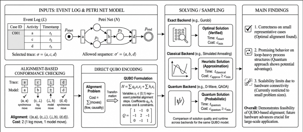
Figure 2.
Running example used throughout this section. The trace fits the lower branch of the Petri net. If the horizon is set to , the optimal alignment can be padded with one filler move.
Figure 2.
Running example used throughout this section. The trace fits the lower branch of the Petri net. If the horizon is set to , the optimal alignment can be padded with one filler move.
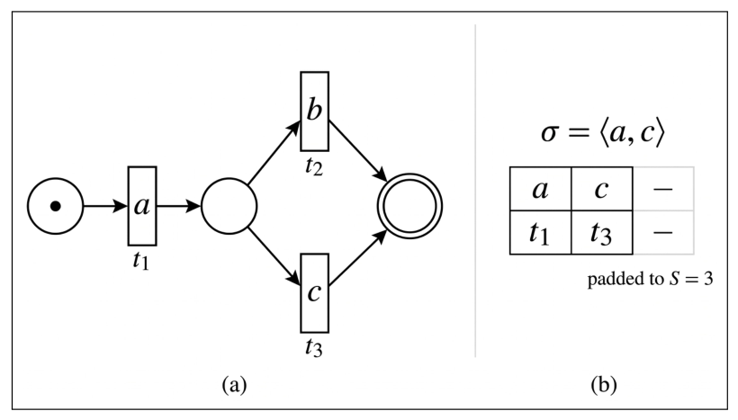
Figure 3.
Fixed-length view of the encoding. Each slot stores the current Petri net state, the current position in the trace, and the action taken in that slot. Shorter alignments are represented by padding with filler moves.
Figure 3.
Fixed-length view of the encoding. Each slot stores the current Petri net state, the current position in the trace, and the action taken in that slot. Shorter alignments are represented by padding with filler moves.
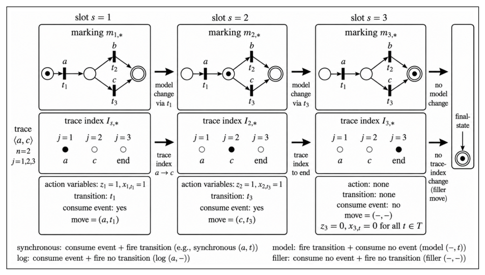
Figure 4.
Three correctness-sensitive situations covered by the benchmark suite: multiple optimal alignments caused by parallelism, zero-cost model moves on silent transitions, and transition-level reasoning in the presence of duplicate visible labels.
Figure 4.
Three correctness-sensitive situations covered by the benchmark suite: multiple optimal alignments caused by parallelism, zero-cost model moves on silent transitions, and transition-level reasoning in the presence of duplicate visible labels.
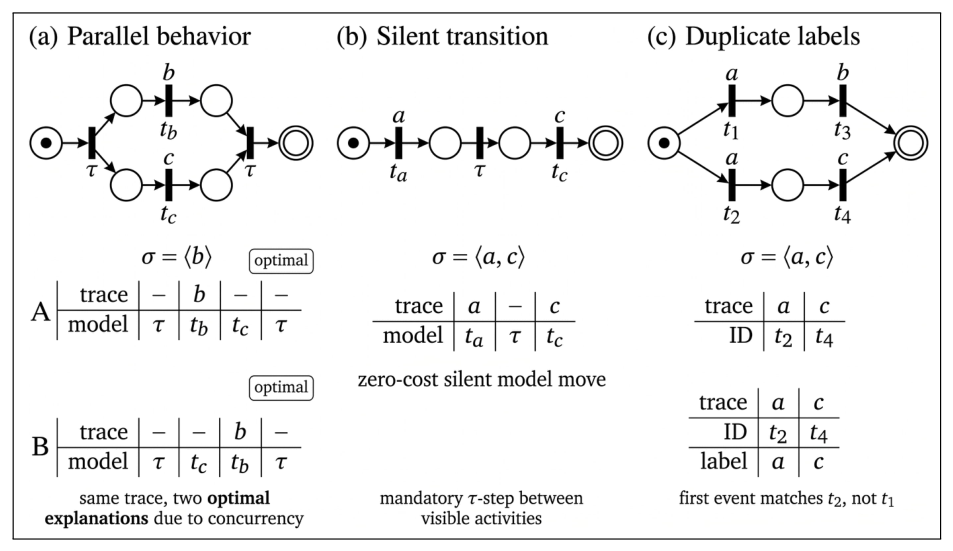
Figure 5.
Recall on the basic correctness benchmark. Since every tested trace in each family had recall 1, the figure reports one aggregated value per benchmark family. The result is based on 5000-sample SA and QPU runs.
Figure 5.
Recall on the basic correctness benchmark. Since every tested trace in each family had recall 1, the figure reports one aggregated value per benchmark family. The result is based on 5000-sample SA and QPU runs.
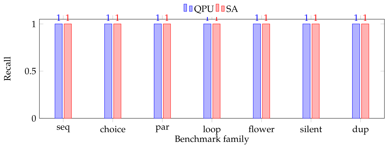
Figure 6.
Schematic summary of the max-S trend. Increasing S increases the logical QUBO approximately linearly, while the embedding grows faster and QPU success drops. For at , the instance has about 205 to 206 logical variables and an embedding of about physical qubits; for , no optimal QPU samples were found.
Figure 6.
Schematic summary of the max-S trend. Increasing S increases the logical QUBO approximately linearly, while the embedding grows faster and QPU success drops. For at , the instance has about 205 to 206 logical variables and an embedding of about physical qubits; for , no optimal QPU samples were found.
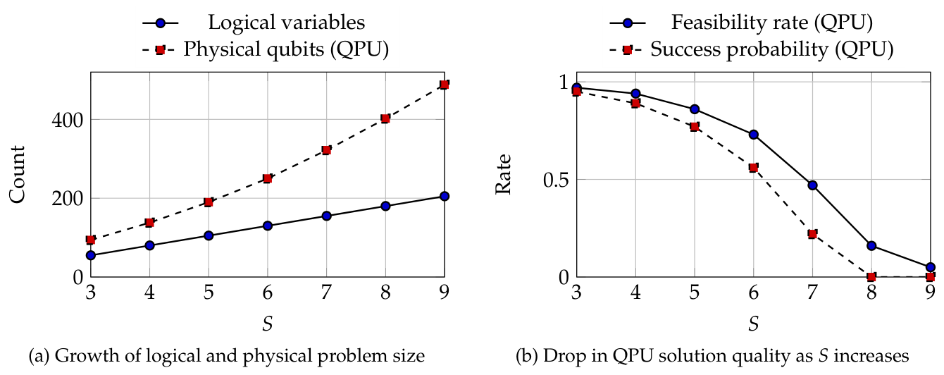
Figure 7.
Why model structure matters: QPU difficulty depends not only on the number of variables but also on the distribution of QUBO interactions. Choice-heavy instances produced more chain stress and chain breaks than modified parallel instances of comparable or larger logical size.
Figure 7.
Why model structure matters: QPU difficulty depends not only on the number of variables but also on the distribution of QUBO interactions. Choice-heavy instances produced more chain stress and chain breaks than modified parallel instances of comparable or larger logical size.
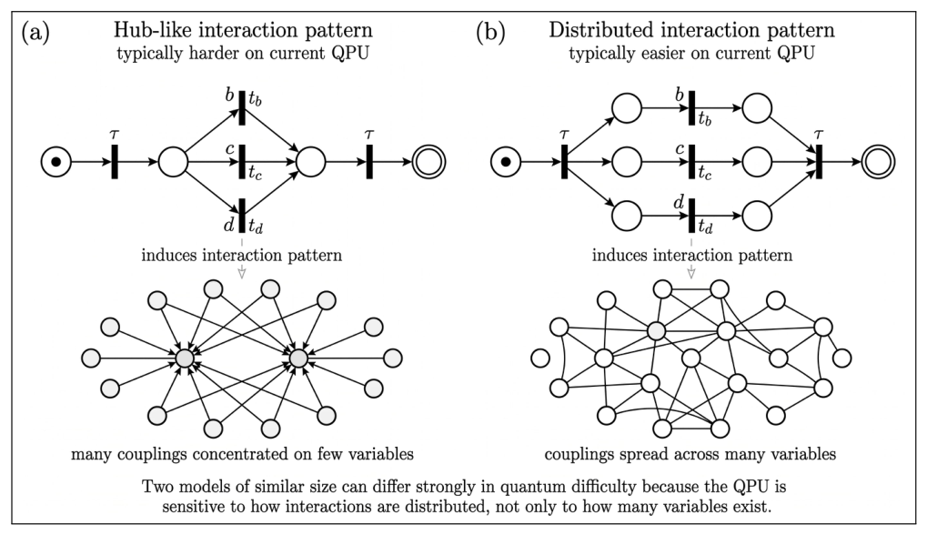
Figure 8.
Representative summary of the loop-based scaling experiment (, fixed and , increasing trace length, varying missing a-activity deviations). The clearest positive QPU signal appears in success probability for traces longer than 3, while the embedding remains favorable with very low chain-break fractions.
Figure 8.
Representative summary of the loop-based scaling experiment (, fixed and , increasing trace length, varying missing a-activity deviations). The clearest positive QPU signal appears in success probability for traces longer than 3, while the embedding remains favorable with very low chain-break fractions.
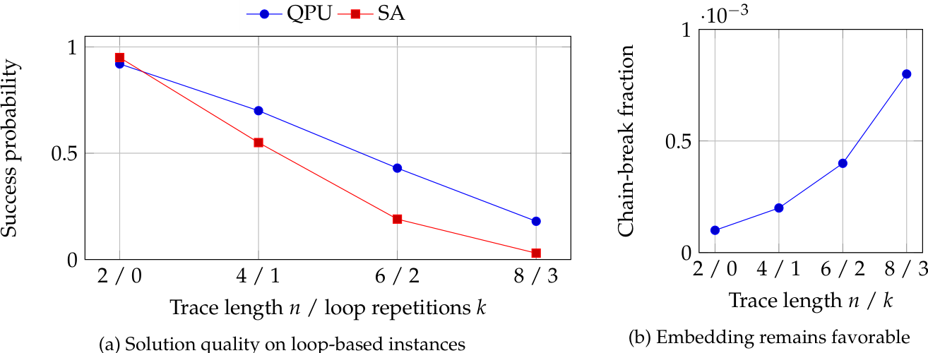
Figure 9.
Interpretation of the loop-based results: the empirical pattern is consistent with the QPU being more effective than simulated annealing on rugged search landscapes, but this is an interpretation rather than a proven mechanism.
Figure 9.
Interpretation of the loop-based results: the empirical pattern is consistent with the QPU being more effective than simulated annealing on rugged search landscapes, but this is an interpretation rather than a proven mechanism.
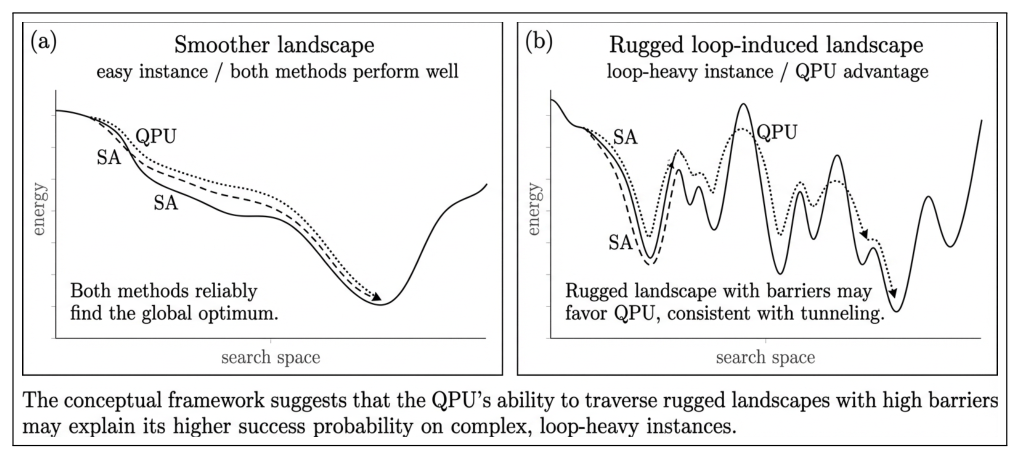
Figure 10.
Why scalability is limited today. A logical alignment QUBO must first be embedded onto the sparse connectivity graph of the QPU. As instances grow, more logical variables require longer and more fragile physical chains.
Figure 10.
Why scalability is limited today. A logical alignment QUBO must first be embedded onto the sparse connectivity graph of the QPU. As instances grow, more logical variables require longer and more fragile physical chains.
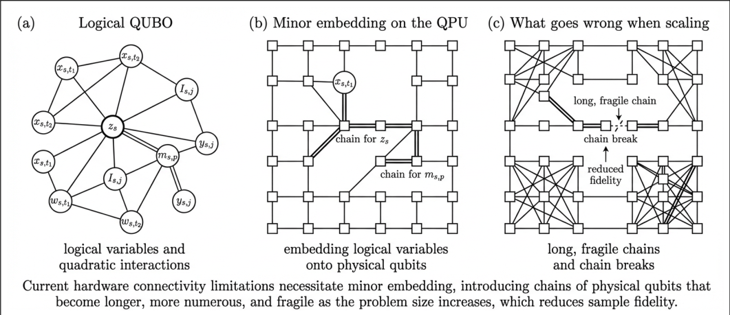
Figure 11.
Evidence that topology is the main bottleneck. The QPU degrades much faster on the choice-heavy instances than on similarly sized modified parallel instances, even though the latter are not smaller in a simple logical sense.
Figure 11.
Evidence that topology is the main bottleneck. The QPU degrades much faster on the choice-heavy instances than on similarly sized modified parallel instances, even though the latter are not smaller in a simple logical sense.
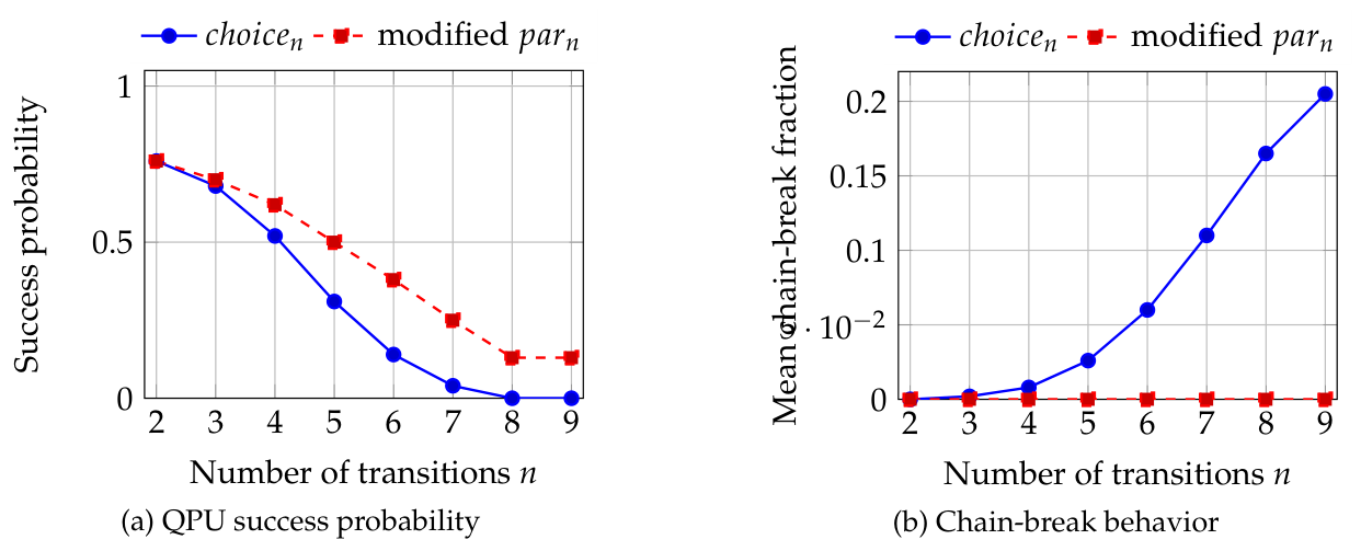

Table 1.
Execution and reference backends used in the evaluation.
| Tool | Role | Default setting |
|---|---|---|
| QPU | Quantum annealing backend | D-Wave Advantage2 system; 5000 anneals; default annealing time ; Ocean SDK defaults unless stated otherwise |
| SA | Classical stochastic baseline | 5000 samples; 500 sweeps per sample |
| SCIP | Exact solver | linearized QUBO; default settings |
| PM4Py | Independent alignment reference | used to cross-check optimal alignment costs on the benchmark instances |
Table 2.
Representative correctness scenarios covered by the benchmark suite.
| Scenario | What it tests | Main observation |
|---|---|---|
| Pure sequential behavior | Expected optimal alignments recovered for fitting and non-fitting traces. | |
| Exclusive branching | Fitting branches and wrong-branch deviations correctly distinguished. | |
| Parallel behavior | All distinct optimal alignments recovered; concurrency not collapsed into one answer. | |
| Repetition and local ambiguity | Optimal alignments recovered despite several near-optimal loop-related explanations. | |
| Very permissive behavior | Correct optimum returned although the model admits many alternative explanations. | |
| Silent-transition variant | Silent model moves | Zero-cost model moves on -transitions correctly allowed. |
| Duplicate-label variant | Non-unique visible labels | Transitions sharing the same visible label are distinguished. |
Table 3.
Interpretive summary of the main difficulty drivers observed in the evaluation.
| Factor | What changes | Main observed effect | Importance |
|---|---|---|---|
| Horizon S | Number of slots in the encoding | Larger QUBOs, larger embeddings, lower feasibility and lower success probability | High |
| Model structure | Distribution of interactions in the QUBO | Hub-like structures are harder than more distributed ones, even at similar scale | High |
| Trace length | Size of trace-index encoding and number of possible deviations | Larger and less regular search spaces, especially in loop-based models | Medium |
Table 4.
Simple summary of where the QPU helps in the current evaluation.
| Instance type | QPU relative to SA | Interpretation |
|---|---|---|
| Small and easy instances | Roughly similar | Both methods already find the optimum reliably |
| Large or embedding-heavy instances | Usually worse | Physical embedding problems dominate on the QPU |
| Loop-heavy instances with still-manageable embeddings | Better on success probability | Most promising early signal for quantum annealing |
Table 5.
Main scalability bottlenecks observed in the evaluation.
| Bottleneck | Why it appears | Effect on alignment computation |
|---|---|---|
| Sparse hardware connectivity | Logical interactions cannot be mapped directly to the QPU graph | More chains and more physical qubits are needed |
| Long or stressed chains | Larger or more hub-like QUBOs are harder to embed | More chain breaks, lower feasibility, lower success probability |
| Interaction concentration | Some process structures create highly connected logical variables | Quality can collapse even when the logical problem is not extremely large |
| Fixed horizon S | The alignment length must be bounded in advance | Too small excludes the optimum; too large worsens scaling |
Disclaimer/Publisher’s Note: The statements, opinions and data contained in all publications are solely those of the individual author(s) and contributor(s) and not of MDPI and/or the editor(s). MDPI and/or the editor(s) disclaim responsibility for any injury to people or property resulting from any ideas, methods, instructions or products referred to in the content. |
© 2026 by the authors. Licensee MDPI, Basel, Switzerland. This article is an open access article distributed under the terms and conditions of the Creative Commons Attribution (CC BY) license (http://creativecommons.org/licenses/by/4.0/).
Copyright: This open access article is published under a Creative Commons CC BY 4.0 license, which permit the free download, distribution, and reuse, provided that the author and preprint are cited in any reuse.


