

Submitted:
03 July 2026
Posted:
07 July 2026
You are already at the latest version
Abstract
Process mining revolves around heterogeneous artifacts: event logs record observed behavior, while process trees and Petri nets specify intended or discovered behavior. Every established technique that connects two of these artifact types-process discovery, conformance checking, model transformation-is a dedicated algorithm for one direction of one artifact pair. This paper presents ProcRosetta, a multimodal neural framework that embeds event logs, process trees, and Petri nets into a single shared latent space of process behavior and decodes any point of that space into a syntactically valid process tree. Three artifact-specific encoders (a recurrent tree encoder, a hierarchical attention-based log encoder, and a message-passing Petri-net encoder) are trained jointly with a shared grammar-masked decoder on synthetic paired triples, using reconstruction, cross-modal translation, latent alignment, contrastive, and variational objectives; grammar masking and deterministic tree-to-net conversion make every generated model well-formed by construction. On a held-out test set of 512 process triples, ProcRosetta decodes valid, Petri-convertible process trees from all three modalities in 100\% of the cases, translates unseen event logs into process models that reach an alignment-based F1 of 0.787 (compared to 0.857 for the Inductive Miner), retrieves cross-modal counterparts far above chance level, and produces 64-dimensional embeddings whose geometry correlates with behavioral distance on par with much higher-dimensional deterministic log representations. The implementation, data generator, and evaluation suite are publicly available.
Keywords:
process mining
; representation learning
; process trees
; Petri nets
; event logs
; multimodal learning
; grammar-constrained decoding
1. Introduction
Process mining connects observed event data with formal process models [1] and constantly moves between different representations of the same behavior: an event log is a finite sample of executed traces, a process tree is a block-structured hierarchical specification, and a Petri net is a graph-based execution model with explicit states and concurrency. The bridges between these views are dedicated, hand-designed algorithms, each for one direction of one artifact pair: discovery maps logs to models [2,3,4], conformance checking relates logs and models through alignments [5], and model-to-model transformations connect notations such as workflow nets and process trees [6]. What is missing is a common computational representation in which a log, a process tree, and a Petri net describing the same behavior are simply the same point. Such a representation would enable similarity search and clustering across artifact types, provide fixed-length behavioral feature vectors for downstream machine learning, and turn translation between artifact types into a decode operation. In machine learning, embedding heterogeneous modalities such as images and text into one shared vector space has proven remarkably effective [7,8]; process mining has adopted representation learning for traces and logs [9,10] and for Petri nets [11], but these efforts remain single-modality, and none of them can generate a process model back from the learned space.
This paper presents ProcRosetta, a multimodal neural framework that treats event logs, process trees, and Petri nets as three views of one process behavior. ProcRosetta trains three artifact-specific encoders into a shared latent space, aligns the views of the same process through explicit alignment and contrastive objectives, and attaches a single shared decoder that maps any latent vector back to a process tree. The decoder is grammar-masked: at every generation step, only tokens that keep the partial output a syntactically valid process tree are allowed, following the philosophy of grammar-constrained decoding [12,13]; decoded trees are converted to Petri nets deterministically using PM4Py [14], so every generated model is well-formed and sound by construction. The name is an analogy to the Rosetta stone: the training data is the same content in three “languages”, and the model learns the correspondence.
Figure 1 summarizes the framework. Three research questions organize the investigation:
- RQ1
- Can event logs, process trees, and Petri nets be embedded into a shared latent space in which the three views of the same process behavior receive nearby representations?
- RQ2
- Can a learned model translate event logs or Petri nets into valid process trees—well-formed, Petri-convertible models whose behavior is close to the source?
- RQ3
- How do the learned representations and the learned log-to-model translation compare with classical baselines: deterministic log and model features, Petri-net embeddings, and the Inductive Miner?
The contributions are: (i) a multimodal architecture with three artifact-specific encoders projecting into one latent space of process behavior; (ii) a shared, grammar-masked process-tree decoder that guarantees syntactic validity of every generated model and, through deterministic conversion, yields sound Petri nets; (iii) a training procedure over synthetic paired triples combining reconstruction, cross-modal translation, latent alignment, contrastive, and variational objectives; and (iv) a comprehensive assessment with a publicly available implementation, covering decode quality, discovery quality against the Inductive Miner, behavior-aligned embedding quality, and cross-modal retrieval.
2. Related Work
- Process discovery and block-structured models.
Automated process discovery derives a process model from an event log [2]; a large benchmark over real-life logs showed that no single algorithm dominates across fitness, precision, generalization, and simplicity [15]. The Inductive Miner [3] discovers process trees by recursive log decomposition, yielding block-structured models that are sound by construction; process trees are a standard pivot representation with formal conversions to Petri nets and BPMN [16], and workflow nets can be translated back to process trees when possible [6]. Beyond strict block structure, Split Miner [4] balances accuracy and simplicity, and the POWL family [17,18] discovers partially ordered workflow models that are more expressive than process trees while preserving soundness. ProcRosetta shares the Inductive Miner’s process-tree bias—the decoder emits process trees because their grammar guarantees well-formedness and their Petri-net conversion is deterministic—but instead of a deterministic log-to-model algorithm, it learns a shared representation over logs, trees, and nets from which models can be decoded.
- Model similarity, conformance, and behavioral distances.
Similarity of process models has been measured over labels, structure, and behavior [19], with the recurring insight that behavioral closeness cannot be reduced to structural resemblance; alignment-based conformance checking [5] provides exact, interpretable comparisons between logs and models. ProcRosetta learns a continuous proxy for such comparisons—attractive for scalable retrieval and clustering, but without formal guarantees—so the assessment measures explicitly how well the learned geometry agrees with a behavioral distance (Section 5.4).
- Representation learning for process-mining artifacts.
Representation learning entered process mining chiefly through single-modality embeddings: act2vec, trace2vec, log2vec, and model2vec [9] and a rich design space of trace encodings [10]. Deep sequence models for predictive monitoring [20] learn powerful trace representations but target prediction over running cases rather than model generation or cross-artifact alignment. On the model side, Petri nets are graphs, making random-walk embeddings such as node2vec [21] and graph neural networks [22] relevant. Most directly related is PetriNet2Vec by Colonna et al. [11], which learns unsupervised vector representations of Petri nets and serves as a baseline in our assessment. All of these approaches embed one artifact family; ProcRosetta’s distinctive step is to align three artifact families in one space and to couple the space with a generative decoder.
- Neural and LLM-based process-model generation.
Sommers et al. [23] train graph neural networks on synthetic log–model pairs to discover sound Petri nets; this is the closest neural predecessor, though it addresses one direction (log→net) rather than a tri-modal space. More recently, large language models have been used to generate process models from natural-language descriptions [24], also specialized via reinforcement learning with verifiable rewards [25]. These approaches are language-native, whereas ProcRosetta is artifact-native—its inputs are logs, trees, and nets themselves—so the directions are complementary.
- Multimodal learning and grammar-constrained decoding.
Outside process mining, multimodal learning studies shared representations across modalities [8]; CLIP [7] demonstrated contrastive alignment of paired images and captions at scale. ProcRosetta transfers this recipe to process mining, with the twist that its “modalities” are formal artifacts whose equivalence is behavioral rather than perceptual. For generation, grammar-constrained decoding guarantees syntactic validity of structured outputs, as in grammar variational autoencoders [12] and grammar-constrained LLM decoding [13]; ProcRosetta applies this principle to process trees, combining ideas that have so far been separate—process-tree soundness, graph encoders for Petri nets, log encoders, contrastive multimodal alignment, and grammar-constrained decoding—in a single trainable framework.
3. Preliminaries
We fix a finite alphabet of activity labels . Throughout the paper, activity labels are canonicalized to in order of first occurrence, making all representations invariant to arbitrary activity naming while preserving repeated-activity identity.
- Event logs.
A trace is a finite word with ; an event log is a finite multiset of traces, , preserving trace frequencies. Logs carry only control-flow information here, the classical control-flow abstraction of richer formats such as XES [26].
- Process trees.
A process tree [3,16] is a block-structured process model generated by the grammar
with , where is a visible activity, is a silent step, SEQ executes its children in order, XOR selects exactly one child, AND interleaves its children, and LOOP repeats a body with a redo and an exit part. Every process tree can be converted into a sound workflow net [3]. Since XOR and AND are commutative, their children are sorted by a canonical structural key, giving behaviorally identical permutations one canonical representation.
- Petri nets.
An accepting labeled Petri net [1] is a tuple with places P, transitions T (), flow relation , labeling , and initial and final markings . For neural encoding, a Petri net is represented as a typed graph: each node carries a type (place, visible transition, or invisible transition) and its token counts in and ; each arc carries a direction type. Nodes are sorted by name before tensorization, making the representation deterministic.
4. The ProcRosetta Framework
This section presents the paired training data, the encoders, the grammar-masked decoder, and the training objective, briefly explaining the neural building blocks where they appear.
4.1. Synthetic Paired Triples
Real-world collections rarely record which log, tree, and net represent the same process, so ProcRosetta is trained on synthetic paired triples in which the correspondence holds by construction (Figure 2): each sample is derived from one randomly generated process tree .
- is sampled by a recursive generator that at each node emits an activity leaf (probability , always at maximum depth 3) or an operator from with arity 2 or 3; labels come from at most 30 activities (reuse probability ), and the tree is canonicalized (Section 3);
- is obtained by playing out with PM4Py’s process-tree simulation (16 traces per sample);
- is the typed-graph representation of the Petri net obtained by PM4Py’s deterministic conversion of .
The generator uses a fixed random seed and produces three disjoint splits: 4000 training, 512 validation, and 512 test triples (Table 1). The grammar and the architecture support the LOOP operator as well (Equation (1)); the experiments reported here use the operator set , which covers sequence, exclusive choice, and concurrency.
For neural processing, each artifact is tokenized. A process tree becomes a prefix sequence over a 40-token vocabulary (special tokens, operators, arities, and activities ), where each operator is followed by an explicit arity token and then its children (Figure 2b). Traces are sequences over the 31-token activity vocabulary. The Petri net graph is tensorized into node-type indices, marking features, and two directed adjacency matrices (one per arc direction).
4.2. Three Encoders, One Latent Space
Each encoder maps its artifact to a diagonal Gaussian over a shared -dimensional latent space (), for modality , as in variational autoencoders [27]: is the embedding of the artifact and the encoder’s uncertainty. During training, latent vectors are sampled as with , which regularizes the space; at test time the deterministic mean is used.
Tree encoder. The token sequence of the process tree is embedded and processed by a gated recurrent unit (GRU)—a standard recurrent network that reads a sequence left to right while maintaining a hidden state—with hidden size ; the hidden state at the last non-padding token is projected linearly to .
Log encoder. The event-log encoder is hierarchical, mirroring the log/trace/event structure: a GRU first encodes each trace into a trace vector; an attention mechanism then computes a data-dependent weight for every trace—emphasizing informative trace variants rather than averaging uniformly—and pools the trace vectors into a single log vector, projected to .
Petri-net encoder. The Petri-net encoder is a message-passing graph network [22]. Each node starts from an embedding of its type (place/visible transition/invisible transition) plus a linear encoding of its marking feature; in each of three message-passing rounds, every node updates its vector from its own state and its incoming and outgoing neighbors, followed by a nonlinearity and layer normalization. Mean-pooling over nodes yields the graph vector, projected to . Transition labels are not used as node features, so this encoder captures the structure of the net.
When several views are available, ProcRosetta also defines a fused embedding, the mean .
4.3. Grammar-Masked Process-Tree Decoder
A single decoder, shared by all three modalities, is an autoregressive GRU: the latent vector z initializes its hidden state, and tokens are generated one at a time, each step predicting a distribution over the vocabulary given the tokens so far.
An unconstrained decoder could produce malformed sequences (e.g., an operator without children). ProcRosetta therefore applies a grammar mask derived from a prefix grammar of process trees. The decoding state tracks the number of open node slots and whether an arity token is pending: after , exactly one node is open; an activity or closes one slot; an operator token must be followed by an arity token , which opens k child slots; when no slots remain open, only is valid. At every step, the logits (pre-softmax scores) of all grammar-invalid tokens are set to , so invalid continuations receive zero probability during training and greedy decoding. Consequently, every terminated output parses into a process tree of grammar (1), and PM4Py’s deterministic conversion turns it into a sound Petri net—transferring the validity-by-construction philosophy of grammar-based molecular and program generation [12,13] to process models.
4.4. Training Objective
Training uses teacher forcing: the decoder receives the ground-truth token sequence shifted by one position and learns to predict every next token. Since all three artifacts of a triple share the same target tree, each mini-batch trains three decoding pathways through the same decoder—reconstruction () and two cross-modal translations (, )—via grammar-masked sequence cross-entropies (, , ) with label smoothing distributed only over grammar-valid tokens.
Two objectives shape the latent space. The alignment loss penalizes disagreement between the latent means of the same sample,
pulling the three views of one process toward the same point. The contrastive loss, in the style of CLIP [7], additionally pushes different processes apart: for every modality pair within a mini-batch, a symmetric cross-entropy over cosine similarities (temperature ) rewards each artifact for being most similar to its own counterpart rather than to the other samples in the batch. Finally, a weak KL regularizer toward a standard normal prior [27] keeps the latent space bounded and smooth. The total loss is the weighted sum
Table 2 summarizes the configuration. The model is deliberately small (≈0.5 M parameters), with standard safeguards against overfitting: dropout, weight decay, label smoothing, stochastic latent sampling, validation-based learning-rate reduction, early stopping, and best-validation checkpoint retention.
5. Assessment
The assessment follows the three research questions, covering training behavior, decode quality (RQ2), discovery quality against the Inductive Miner (RQ3), embedding quality against baselines (RQ1, RQ3), and cross-modal retrieval (RQ1). All results are computed on the held-out test split of 512 triples—used neither for optimization nor for model selection—with the best-validation checkpoint and deterministic latent means.
5.1. Training Behavior
Figure 3 shows the training run. Training converged smoothly: the validation loss decreased from to , the schedule halved the learning rate three times (epochs 27, 31, and 38), and early stopping ended the run after epoch 40; the best-validation checkpoint (epoch 35) is used throughout the assessment. The training–validation gap stays small (about at the end), indicating that the regularization suite of Table 2 prevents substantial overfitting. All loss components improve together (Figure 3b): reconstruction is the easiest task; the two translation losses follow at a higher level, as expected, since a log of 16 sampled traces and a label-free net structure carry less information about the target tree than the tree itself; and the contrastive loss drops steeply in the first epochs, showing that separating different processes in latent space is learned early. The test loss of (tree reconstruction , trace→tree , Petri→tree , contrastive ) closely matches the validation loss. Training takes about 30 minutes on a single CPU; no GPU is required at this scale.
5.2. Decode Quality (RQ2)
Table 3 evaluates greedy decoding from all four latent sources. The structural guarantees hold without exception: every one of the 2048 decodes () terminates, parses into a valid process tree, and converts to a Petri net—the direct payoff of grammar masking, answering the syntactic half of RQ2 fully in the affirmative.
The semantic half is more nuanced. The decoded tree exactly equals the canonical target in 48.4% of the cases when decoding from the tree’s own embedding, 40.0% from the log, and 35.9% from the Petri-net structure. Exact match is demanding (a single differing leaf counts as failure); the error-tolerant metrics are more informative: the normalized token edit distance is low (0.18–0.29), and the behavioral distance between the original log and traces simulated from the decoded model ranges from 0.675 to 0.839, whereas the same distance between two unrelated test logs averages 1.566 (Section 5.4)—decoded models are behaviorally about twice as close to their source as a random model of the same distribution. The ordering of sources is intuitive: the tree embedding retains the most information about the tree, then the log, then the label-free Petri structure, with the fused embedding between its constituents.
5.3. Process-Discovery Quality (RQ3)
Table 4 addresses the log-to-model use case: each test log is translated by ProcRosetta (encode the log, decode a tree, convert to a net) and, independently, mined with PM4Py’s Inductive Miner; both models are scored against the log with alignment-based fitness [5] and precision.
The Inductive Miner achieves perfect fitness (1.000) and an F1 of 0.857. This is expected: the test logs are complete, noise-free playouts of block-structured trees—precisely the setting in which the Inductive Miner enjoys rediscovery guarantees [3]—so the comparison is intentionally played on its home turf. ProcRosetta reaches a fitness of 0.841, a precision of 0.763, and an F1 of 0.787—about 92% of the Inductive Miner’s F1. Notably, a purely neural translation—the entire log is compressed into a single 64-dimensional vector, with no search, replay, or counting—lands within this range while producing a valid model for every log. The gap is concentrated in fitness: a slightly wrong decoded tree makes some observed traces non-replayable, whereas the Inductive Miner guarantees their inclusion. We interpret this not as a claim that neural translation should replace classical discovery, but as evidence that the shared latent space preserves enough behavioral information to support discovery-grade model generation.
5.4. Embedding Quality (RQ1, RQ3)
If the latent space is a space of process behavior, then distances in it should correlate with behavioral distances. The assessment quantifies the behavioral distance between two logs as the mean of three distances between empirical distributions extracted from the logs—trace variants, directly-follows relations (with boundary symbols) [28], and trace lengths—each in . Across all pairs of test logs, this distance averages (min , max ). Each embedding method is scored by: (i) the Spearman rank correlation between embedding cosine distance and behavioral distance over all pairs; (ii) the mean behavioral distance from each sample to its nearest neighbor in the embedding (NN behavior; lower is better); and (iii) the improvement of the latter over the random-pair average (higher is better).
Table 5 ranks the four learned ProcRosetta representations against six deterministic baselines and the learned PetriNet2Vec baseline [11]. Three observations stand out. First, the top-ranked method by correlation is the deterministic directly-follows distribution—with a caveat the ranking itself cannot show: the behavioral distance is defined as an average that includes the directly-follows and the trace-variant , so these two baselines partially measure the evaluation target by construction and should be read as skyline references rather than as competing methods. The eventually-follows baseline, which is not part of the distance definition, illustrates how quickly deterministic features degrade otherwise ().
Second, among representations that do not share abstractions with the target metric, ProcRosetta’s log embedding is the strongest all-round performer: with an NN behavior of 0.794—essentially tied with the best skyline baselines on nearest-neighbor quality (0.781–0.784), the operative metric for retrieval-style use cases, while using 64 dimensions instead of 332 (directly-follows) or 2548 (trace variants).
Third, the comparison on the Petri-net side favors ProcRosetta on neighborhoods: PetriNet2Vec attains a good global correlation () but poor nearest neighbors (NN behavior 1.115), whereas ProcRosetta’s net embedding (, NN 0.913) and especially its fused embedding (NN 0.804) retrieve behaviorally much closer neighbors—while the net encoder deliberately ignores transition labels (Section 4.2) and thus solves a harder, purely structural task.
Table 6 adds a geometry-level view, comparing the full pairwise-distance structure of every method against the fused ProcRosetta embedding. The three modality-specific ProcRosetta embeddings agree strongly with each other’s geometry (pairwise of 0.89–0.96 with the fused space) even though they are computed from entirely different inputs—direct evidence for RQ1: the three encoders have converged to one shared geometry of process behavior. In contrast, all external baselines induce substantially different geometries () and share almost no nearest neighbors with the fused space, confirming that the learned space is not a rediscovery of any single deterministic feature set.
5.5. Cross-Modal Retrieval (RQ1)
The most direct test of cross-modal alignment is retrieval: given, e.g., a Petri net, does its embedding find the matching event log among all 512 test logs? Table 7 reports top-1 accuracy, mean reciprocal rank (MRR), and the mean rank of the true counterpart, for all six directions. All directions perform far above chance: top-1 accuracies of 14.1–44.3% against a 0.2% chance level (factors of 70–220), and mean ranks of 32–49 against an expected 256 for random ranking. The pattern is informative: the tree–net pairing is easiest (both artifacts are complete structural descriptions), the tree–log pairing follows, and the log–net pairing is hardest—it connects the two indirect views, a finite behavioral sample and a label-free graph structure, neither of which is the generative object. Distinguishing the one correct process from 511 same-distribution alternatives requires instance-level matching, much finer than the neighborhood-level quality of Section 5.4; the results establish that the shared space aligns modalities at this granularity well above chance, while leaving clear headroom.
5.6. Reproducibility and Implementation
ProcRosetta is implemented in Python on top of PyTorch and PM4Py [14]; the complete source code (synthetic data generator, training and evaluation pipelines, and all metric implementations) is publicly available at https://github.com/fit-alessandro-berti/proc-rosetta. Three commands reproduce the study end-to-end: sample.py regenerates the seeded splits of Table 1, train.py trains the model of Table 2 and writes the per-epoch metrics of Figure 3, and test.py produces every number in Table 3, Table 4, Table 5, Table 6 and Table 7. The repository also provides utilities that apply a trained checkpoint to external artifacts (.xes event logs, .pnml Petri nets, .ptml process trees), computing embeddings and decoding logs or nets into process trees with automatic canonicalization and label restoration.
6. Discussion
- Threats to validity.
Four threats qualify these findings. (i) Synthetic data. Training and evaluation use synthetic triples from random block-structured trees; real logs exhibit noise, incompleteness, deviating behavior, and long-tail variants absent from this distribution, so the conclusions concern in-distribution artifacts (out-of-distribution quality is not claimed here). (ii) Metric circularity. The behavioral distance used for embedding evaluation shares two of its three components with the directly-follows and trace-variant baselines, inflating their scores; Table 5 marks them, and the less affected nearest-neighbor quality is reported alongside correlation. (iii) Duplicate behavior across splits. The generator relies on independent random generation rather than explicit behavioral deduplication, so a fraction of test behaviors may resemble training behaviors; the exact-match rates of Table 3 should be read with this in mind. (iv) Single configuration. All results come from one seeded data configuration and one trained model; variance across seeds and hyperparameter sensitivity are not quantified.
- Scope of the model class.
The operator set used in the experiments covers sequence, exclusive choice, and concurrency; the grammar, tokenizer, and decoder already support the loop operator, so extending the trained model to loops is a data-configuration change rather than an architectural one. More fundamentally, the process-tree target restricts outputs to block-structured behavior—the restriction the Inductive Miner accepts in exchange for soundness—and is less expressive than partially ordered formalisms such as POWL [17,18]. The architecture is modular here: any target language with a prefix grammar, a canonical form, and a deterministic conversion to Petri nets could replace the process-tree decoder.
7. Conclusions
This paper introduced ProcRosetta, a multimodal neural framework that embeds the three central artifact types of process mining—event logs, process trees, and Petri nets—into a single latent space of process behavior and decodes any point of that space into a grammar-valid process tree that converts deterministically into a sound Petri net. The assessment answered all three research questions affirmatively and quantified the remaining headroom: the three encoders converge to one shared geometry that aligns paired artifacts at instance level far above chance (RQ1); grammar-masked decoding produced a valid, Petri-convertible process tree in 100% of 2048 test decodes, with decoded behavior roughly twice as close to the source as unrelated models (RQ2); and the learned 64-dimensional embeddings rival much higher-dimensional deterministic features while log-to-model translation reaches 92% of the Inductive Miner’s F1 in the miner’s own best-case setting (RQ3).
Future work follows directly from the assessment. On the data side: larger and more diverse tree distributions including loops, noisy and incomplete simulated logs, quantified near-duplicate behavior across splits, and validation on real-life logs and model collections. On the model side: label-aware Petri-net encoding, beam or sampling-based decoding, multi-seed robustness studies, and scaling the encoders. On the representation side: richer sound target languages such as POWL [18] as decoder output, an exact-conformance-based evaluation distance, and attaching further encoders—including natural-language process descriptions [24]—to the same latent space, moving closer to a true Rosetta stone for process representations.
Acknowledgments
Funded by the European Union. This work has received funding from the European High Performance Computing Joint Undertaking (JU) and from the German Federal Ministry of Research, Technology and Space (BMFTR), the Ministry of Culture and Science of North Rhine-Westphalia (MKW NRW), and the Hessian Ministry of Science and Research, Arts and Culture (HMWK) under grant agreement No 101250682.
References
- van der Aalst, W.M.P. Process Mining—Data Science in Action, 2nd ed.; Springer: Berlin/Heidelberg, Germany, 2016. [Google Scholar]
- van der Aalst, W.M.P.; Weijters, T.; Maruster, L. Workflow Mining: Discovering Process Models from Event Logs. IEEE Trans. Knowl. Data Eng. 2004, 16, 1128–1142. [Google Scholar] [CrossRef]
- Leemans, S.J.J.; Fahland, D.; van der Aalst, W.M.P. Discovering Block-Structured Process Models from Event Logs—A Constructive Approach. In Proceedings of the PETRI Nets; Lecture Notes in Computer Science; Springer: Berlin/Heidelberg, Germany, 2013; Volume 7927, pp. 311–329. [Google Scholar]
- Augusto, A.; Conforti, R.; Dumas, M.; Rosa, M.L.; Polyvyanyy, A. Split miner: Automated discovery of accurate and simple business process models from event logs. Knowl. Inf. Syst. 2019, 59, 251–284. [Google Scholar]
- Adriansyah, A.; Munoz-Gama, J.; Carmona, J.; van Dongen, B.F.; van der Aalst, W.M.P. Alignment Based Precision Checking. In Proceedings of the Business Process Management Workshops; Lecture Notes in Business Information Processing; Springer: Berlin/Heidelberg, Germany, 2012; Volume 132, pp. 137–149. [Google Scholar]
- van Zelst, S.J.; Leemans, S.J.J. Translating Workflow Nets to Process Trees: An Algorithmic Approach. Algorithms 2020, 13, 279. [Google Scholar] [CrossRef]
- Radford, A. Learning Transferable Visual Models From Natural Language Supervision. In Proceedings of the ICML; Proceedings of Machine Learning Research; JMLR: Cambridge, MA, USA, 2021; Volume 139, pp. 8748–8763. [Google Scholar]
- Baltrusaitis, T.; Ahuja, C.; Morency, L. Multimodal Machine Learning: A Survey and Taxonomy. IEEE Trans. Pattern Anal. Mach. Intell. 2019, 41, 423–443. [Google Scholar] [PubMed]
- Koninck, P.D.; vanden Broucke, S.; Weerdt, J.D. act2vec, trace2vec, log2vec, and model2vec: Representation Learning for Business Processes. In Proceedings of the BPM; Lecture Notes in Computer Science; Springer: Cham, Switzerland, 2018; Volume 11080, pp. 305–321. [Google Scholar]
- Tavares, G.M.; Oyamada, R.S.; Barbon, S.; Ceravolo, P. Trace encoding in process mining: A survey and benchmarking. Eng. Appl. Artif. Intell. 2023, 126, 107028. [Google Scholar] [CrossRef]
- Colonna, J.G.; Fares, A.A.; Duarte, M.; Sousa, R.T. Process mining embeddings: Learning vector representations for Petri nets. Intell. Syst. Appl. 2024, 23, 200423. [Google Scholar] [CrossRef]
- Kusner, M.J.; Paige, B.; Hernández-Lobato, J.M. Grammar Variational Autoencoder. In Proceedings of the ICML; Proceedings of Machine Learning Research; JMLR: Cambridge, MA, USA, 2017; Volume 70, pp. 1945–1954. [Google Scholar]
- Geng, S.; Josifoski, M.; Peyrard, M.; West, R. Grammar-Constrained Decoding for Structured NLP Tasks without Finetuning. In Proceedings of the EMNLP; Association for Computational Linguistics: Stroudsburg, PA, USA, 2023; pp. 10932–10952. [Google Scholar]
- Berti, A.; van Zelst, S.J.; Schuster, D. PM4Py: A process mining library for Python. Softw. Impacts 2023, 17, 100556. [Google Scholar] [CrossRef]
- Augusto, A.; Conforti, R.; Dumas, M.; Rosa, M.L.; Maggi, F.M.; Marrella, A.; Mecella, M.; Soo, A. Automated Discovery of Process Models from Event Logs: Review and Benchmark. IEEE Trans. Knowl. Data Eng. 2019, 31, 686–705. [Google Scholar]
- Leemans, S.J.J.; van Zelst, S.J.; Lu, X. A Brief Overview of Process Trees. In Proceedings of the Mining a Scientist’s Process; Lecture Notes in Computer Science; Springer: Cham, Switzerland, 2026; Volume 16480, pp. 315–332. [Google Scholar]
- Kourani, H.; van Zelst, S.J. POWL: Partially Ordered Workflow Language. In Proceedings of the BPM; Lecture Notes in Computer Science; Springer: Cham, Switzerland, 2023; Volume 14159, pp. 92–108. [Google Scholar]
- Kourani, H.; Park, G.; van der Aalst, W.M.P. A discovery technique for expressive yet sound process models. Process Sci. 2026, 3, 14. [Google Scholar] [CrossRef]
- Dijkman, R.M.; Dumas, M.; van Dongen, B.F.; Käärik, R.; Mendling, J. Similarity of business process models: Metrics and evaluation. Inf. Syst. 2011, 36, 498–516. [Google Scholar] [CrossRef]
- Rama-Maneiro, E.; Vidal, J.C.; Lama, M. Deep Learning for Predictive Business Process Monitoring: Review and Benchmark. IEEE Trans. Serv. Comput. 2023, 16, 739–756. [Google Scholar]
- Grover, A.; Leskovec, J. node2vec: Scalable Feature Learning for Networks. In Proceedings of the KDD; ACM: New York, NY, USA, 2016; pp. 855–864. [Google Scholar]
- Kipf, T.N.; Welling, M. Semi-Supervised Classification with Graph Convolutional Networks. In Proceedings of the ICLR (Poster); OpenReview.net: Alameda, CA, USA, 2017. [Google Scholar]
- Sommers, D.; Menkovski, V.; Fahland, D. Supervised learning of process discovery techniques using graph neural networks. Inf. Syst. 2023, 115, 102209. [Google Scholar] [CrossRef]
- Kourani, H.; Berti, A.; Schuster, D.; van der Aalst, W.M.P. Process Modeling with Large Language Models. In Proceedings of the BPMDS/EMMSAD@CAiSE; Lecture Notes in Business Information Processing; Springer: Cham, Switzerland, 2024; Volume 511, pp. 229–244. [Google Scholar]
- Berti, A.; Wang, X.; Kourani, H.; van der Aalst, W.M.P. Specializing large language models for process modeling via reinforcement learning with verifiable and universal rewards. Process Sci. 2025, 2, 26. [Google Scholar] [CrossRef]
- IEEE Std 1849-2023; IEEE Standard for eXtensible Event Stream (XES) for Achieving Interoperability in Event Logs and Event Streams. IEEE: New York, NY, USA, 2023.
- Kingma, D.P.; Welling, M. Auto-Encoding Variational Bayes. In Proceedings of the ICLR, Banff, AB, Canada, 14–16 April 2014. [Google Scholar]
- van der Aalst, W.M.P. A practitioner’s guide to process mining: Limitations of the directly-follows graph. In Proceedings of the CENTERIS/ProjMAN/HCist; Procedia Computer Science; Elsevier: Amsterdam, The Netherlands, 2019; Volume 164, pp. 321–328. [Google Scholar]
Figure 1.
Overview of ProcRosetta. Stage 1 (encoding): three views of one process behavior are mapped by artifact-specific encoders into a shared latent space, where alignment and contrastive objectives pull views of the same process together and push different processes apart; the embeddings support cross-artifact similarity search, clustering, and downstream machine learning. Stage 2 (decoding): a shared grammar-masked decoder maps any latent vector to a syntactically valid process tree, deterministically convertible to a Petri net—realizing auto-encoding (tree→tree), process discovery (log→tree), or model translation (net→tree).
Figure 1.
Overview of ProcRosetta. Stage 1 (encoding): three views of one process behavior are mapped by artifact-specific encoders into a shared latent space, where alignment and contrastive objectives pull views of the same process together and push different processes apart; the embeddings support cross-artifact similarity search, clustering, and downstream machine learning. Stage 2 (decoding): a shared grammar-masked decoder maps any latent vector to a syntactically valid process tree, deterministically convertible to a Petri net—realizing auto-encoding (tree→tree), process discovery (log→tree), or model translation (net→tree).
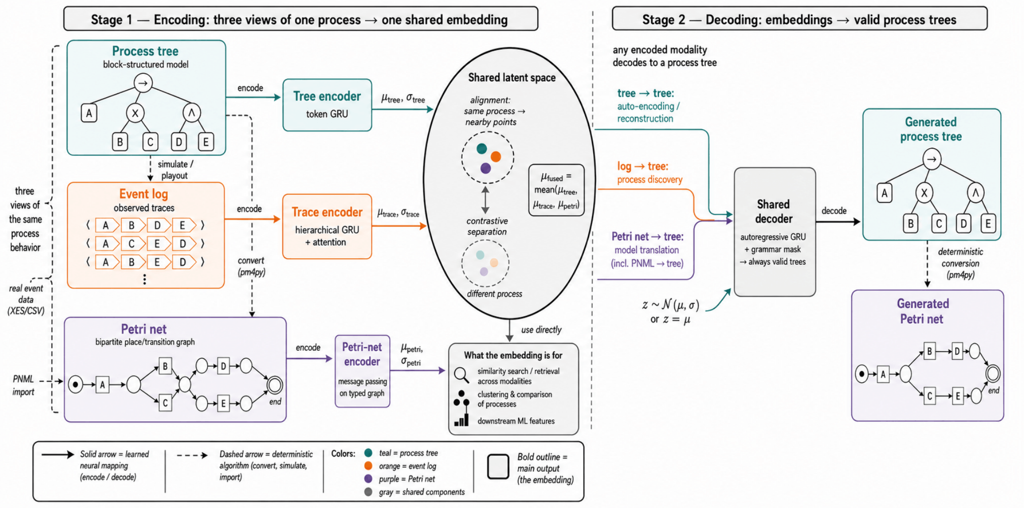
Figure 2.
One synthetic paired triple: a generated process tree (a) is serialized as a prefix token sequence with explicit arities (b), simulated into an event log (c); superscripts denote trace frequencies), and deterministically converted into an accepting Petri net (d).
Figure 2.
One synthetic paired triple: a generated process tree (a) is serialized as a prefix token sequence with explicit arities (b), simulated into an event log (c); superscripts denote trace frequencies), and deterministically converted into an accepting Petri net (d).

Figure 3.
Training behavior. (a) Training and validation loss per epoch; dashed lines mark learning-rate halvings on validation plateaus, the dotted line the best-validation checkpoint (epoch 35) used in all evaluations. (b) The validation loss components decrease jointly.
Figure 3.
Training behavior. (a) Training and validation loss per epoch; dashed lines mark learning-rate halvings on validation plateaus, the dotted line the best-validation checkpoint (epoch 35) used in all evaluations. (b) The validation loss components decrease jointly.
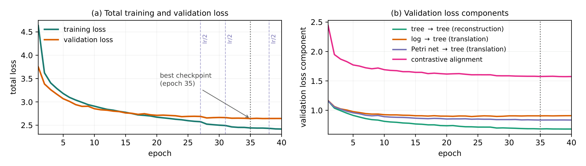

Table 1.
Synthetic dataset statistics per split (each sample is a paired triple; fixed seed).
| Split | Samples | Avg. Tree Size |
Avg. Tree Depth |
Traces per Sample |
Avg. Trace Length |
Max Petri Nodes |
Max Petri Edges |
|---|---|---|---|---|---|---|---|
| Training | 4000 | 10.31 | 3.18 | 16 | 3.97 | 63 | 78 |
| Validation | 512 | 10.30 | 3.18 | 16 | 3.81 | 55 | 68 |
| Test | 512 | 10.63 | 3.18 | 16 | 3.95 | 58 | 70 |
Table 2.
Model and training configuration.
| Architecture | Optimization | ||
|---|---|---|---|
| Latent dimension | 64 | Optimizer | AdamW (lr , weight decay ) |
| Hidden dimension H | 128 | Batch size | 32 |
| Dropout | 0.15 | Gradient clipping | global norm 5.0 |
| Petri message-passing rounds | 3 | Label smoothing | 0.05 |
| Vocabularies | 40 tree/31 act. tokens | LR schedule | halve on val. plateau (patience 2) |
| Trainable parameters | 524,713 | Early stopping | patience 5 of max. 100 epochs |
Table 3.
Decode quality on the test split (512 samples), greedy decoding from each latent source. Norm. edit: length-normalized token edit distance; behavior : original log vs. traces simulated from the decoded tree (range ; unrelated test logs average 1.566). Lower is better for both.
Table 3.
Decode quality on the test split (512 samples), greedy decoding from each latent source. Norm. edit: length-normalized token edit distance; behavior : original log vs. traces simulated from the decoded tree (range ; unrelated test logs average 1.566). Lower is better for both.
| Latent Source | Terminated | Valid Tree | Exact Tree | Petri Conv. | Norm. Edit ↓ | Behavior ↓ |
|---|---|---|---|---|---|---|
| (tree encoder) | 100% | 100% | 48.4% | 100% | 0.178 | 0.675 |
| (log encoder) | 100% | 100% | 40.0% | 100% | 0.287 | 0.755 |
| (Petri encoder) | 100% | 100% | 35.9% | 100% | 0.282 | 0.839 |
| (mean of the three) | 100% | 100% | 44.3% | 100% | 0.230 | 0.713 |
Table 4.
Process-discovery quality on the 512 test logs: the model decoded from the log embedding (ProcRosetta) and the Inductive Miner model are evaluated against each log with alignment-based fitness and precision; F1 is their harmonic mean.
Table 4.
Process-discovery quality on the 512 test logs: the model decoded from the log embedding (ProcRosetta) and the Inductive Miner model are evaluated against each log with alignment-based fitness and precision; F1 is their harmonic mean.
| Method | Model Obtained | Alignments Computable | Fitness | Precision | F1 |
|---|---|---|---|---|---|
| ProcRosetta (log → tree → net) | 100% | 100% | 0.841 | 0.763 | 0.787 |
| Inductive Miner | 100% | 100% | 1.000 | 0.797 | 0.857 |
Table 5.
Embedding quality on the test split, ranked by Spearman correlation between embedding distance and behavioral distance over all 130,816 pairs. NN behavior: mean behavioral distance to the nearest embedding neighbor; Improv.: improvement over the random-pair mean (1.566). •: learned; ∘: deterministic features; †: shares abstractions with the behavioral-distance definition itself.
Table 5.
Embedding quality on the test split, ranked by Spearman correlation between embedding distance and behavioral distance over all 130,816 pairs. NN behavior: mean behavioral distance to the nearest embedding neighbor; Improv.: improvement over the random-pair mean (1.566). •: learned; ∘: deterministic features; †: shares abstractions with the behavioral-distance definition itself.
| Method | Type | Dim. | Behavior ↑ | NN Behavior ↓ | Improv. ↑ |
|---|---|---|---|---|---|
| Directly-follows distribution † | ∘ log features | 332 | 0.736 | 0.784 | 0.782 |
| PetriNet2Vec (PM4Py) [11] | • learned (net) | 64 | 0.643 | 1.115 | 0.451 |
| Activity counts | ∘ log features | 20 | 0.635 | 0.946 | 0.620 |
| ProcRosetta | • learned (log) | 64 | 0.630 | 0.794 | 0.772 |
| ProcRosetta | • learned (all) | 64 | 0.628 | 0.804 | 0.761 |
| PM4Py log case features | ∘ log features | 40 | 0.619 | 0.821 | 0.745 |
| Trace-variant distribution † | ∘ log features | 2548 | 0.614 | 0.781 | 0.785 |
| ProcRosetta | • learned (tree) | 64 | 0.611 | 0.836 | 0.730 |
| ProcRosetta | • learned (net) | 64 | 0.574 | 0.913 | 0.652 |
| Petri structural counts | ∘ net features | 9 | 0.439 | 0.925 | 0.640 |
| Eventually-follows distribution | ∘ log features | 347 | 0.412 | 0.881 | 0.685 |
Table 6.
Geometry agreement with the fused ProcRosetta embedding: Spearman correlation of pairwise-distance matrices, top-1 nearest-neighbor overlap, and deltas versus the fused reference (negative NN behavior = better neighborhoods).
Table 6.
Geometry agreement with the fused ProcRosetta embedding: Spearman correlation of pairwise-distance matrices, top-1 nearest-neighbor overlap, and deltas versus the fused reference (negative NN behavior = better neighborhoods).
| Method | Pairwise | Top-1 NN Overlap | Behavior | NN Behavior |
|---|---|---|---|---|
| ProcRosetta | 0.960 | 0.320 | ||
| ProcRosetta | 0.951 | 0.283 | ||
| ProcRosetta | 0.890 | 0.316 | ||
| PetriNet2Vec (PM4Py) | 0.669 | 0.037 | ||
| Petri structural counts | 0.618 | 0.150 | ||
| PM4Py log case features | 0.546 | 0.088 | ||
| Trace-variant distribution | 0.501 | 0.039 | ||
| Directly-follows distribution | 0.488 | 0.102 | ||
| Activity counts | 0.417 | 0.174 | ||
| Eventually-follows distribution | 0.337 | 0.055 |
Table 7.
Cross-modal retrieval on the test split: the 512 candidates of the target modality are ranked by cosine similarity to the query embedding. Chance level: top-1 , mean rank .
Table 7.
Cross-modal retrieval on the test split: the 512 candidates of the target modality are ranked by cosine similarity to the query embedding. Chance level: top-1 , mean rank .
| Query → Target | Top-1 Accuracy | MRR | Mean Rank |
|---|---|---|---|
| tree → net | 44.3% | 0.523 | 36.2 |
| net → tree | 34.2% | 0.442 | 38.0 |
| tree → log | 29.3% | 0.383 | 32.4 |
| log → tree | 25.6% | 0.354 | 33.2 |
| net → log | 15.4% | 0.236 | 49.4 |
| log → net | 14.1% | 0.236 | 48.2 |
Disclaimer/Publisher’s Note: The statements, opinions and data contained in all publications are solely those of the individual author(s) and contributor(s) and not of MDPI and/or the editor(s). MDPI and/or the editor(s) disclaim responsibility for any injury to people or property resulting from any ideas, methods, instructions or products referred to in the content. |
© 2026 by the authors. Licensee MDPI, Basel, Switzerland. This article is an open access article distributed under the terms and conditions of the Creative Commons Attribution (CC BY) license (http://creativecommons.org/licenses/by/4.0/).
Copyright: This open access article is published under a Creative Commons CC BY 4.0 license, which permit the free download, distribution, and reuse, provided that the author and preprint are cited in any reuse.


