

Submitted:
06 July 2026
Posted:
07 July 2026
You are already at the latest version
Abstract
The energy transition towards low emissions is crucial to mitigating climate change. Governments need to enforce policy packages to advance climate goals with speed. This paper presents a methodology for prioritizing policy options that transform energy systems into highly renewable in a long-term planning horizon, considering the interaction of decarbonization and production sophistication (or economic complexity). Governments, businesses, and citizens are aware of the importance of energy transformations. However, understanding the effects and trade-offs of each policy option is yet open to much public debate at municipal, regional, national, or supranational levels. Our methodology offers a practical approach to inform such discussion. We measure each option with four metrics: emission reductions, economic benefits, cost, and the cost reduction of firms that increase the economy's complexity. We apply it by systematically comparing climate mitigation options in transport, electricity, and industry subsectors of the Costa Rican energy system. We find that electrifying road freight and private passenger transport and implementing passenger mode shift and rail achieve 69% of total potential avoided emissions. They also cause 2.2% of GDP in economic benefits (yearly 2021-50 average) and reduce firms' costs that increase the economy's complexity by 0.19% of GDP (yearly 2021-50 average).
Keywords:
decarbonization
; renewable energy systems
; energy transition
; climate change mitigation
; energy system modeling
; economic competitiveness
1. Introduction
Comprehensive long-term transformations to resilient and low emissions economies can be economically beneficial [1]. For example, some Latin American countries have recently carried out cost-benefit analyses of decarbonization strategies, quantifying their economic benefits at US$41 billion in Costa Rica [2,3], US$140 billion in Peru [3], and an additional 0.8% of Gross Domestic Product (GDP) growth in Chile [4]. Such decarbonization strategies largely depend on transitioning from fossil to renewable energy [1]. Whether 100% renewable energy systems are necessary, convenient, and possible for a country depends on its resources, context [5,6], and technological challenges [7]. Notwithstanding the specific cases, some studies have observed that energy production renewability aligned with production sophistication (i.e., higher economic complexity [8,9]) diminishes environmental degradation [10,11,12] – including greenhouse gas (GHG) emissions driving climate change.
The literature has explored econometric relationships between growth, economic complexity, renewability, and emissions. In Europe, renewable energy consumption is more favorable for economic growth than non-renewable consumption, with economic complexity, trade openness, foreign direct investment, and institutional quality as influencing factors [13]. In turn, economic complexity and renewability diminish emissions [10]. However, countries with lower still-growing economic complexity may need more stringent renewable energy policies to avoid high pollution risks [14]. In G7 countries, political uncertainty can enlarge the effects of high energy intensities on high pollution levels [15]. In BRICS economies (Brazil, Russia, India, China, and South Africa) [11] and the sixteen largest exporting economies [12], increases in economic complexity and renewable energy improve climate change mitigation contribution. Moreover, preparedness to export low-emission products competitively can predict lower emissions country-wise [16]. Such preparedness for a low-carbon transition varies across counties [17].
Successfully implementing decarbonization needs overcoming political and economic challenges [18]: managing the jobs transition, avoiding a rise of inequality, carrying forward adequate investments, and sustained political and public support [19]. Ideally, decarbonization will advance job creation in new sectors, outpacing the jobs lost in fossil-based activities [20], even as a measure for the COVID-19 pandemic recovery [21]. Nevertheless, there is another way to look at the holistic low-carbon development paradigm: governments prioritize the decarbonization policies that simultaneously drive emissions to zero and increase the country’s economic complexity. The higher complexity the production structure of an economy has, the more high-value exports, growth, and prosperity it produces [8].
Under such a paradigm, politicians and firms will advance decarbonization if the value chain of a high-value product (i.e., an economically complex structure) becomes more cost-efficient, which can occur, for example, with low-cost renewables [22]. The avoided costs from environmental damage and natural resource depletion increase the benefits of decarbonization and renewables [23].
Despite most literature focusing on final state analyses, highly renewable energy systems need planning the transition [5]. Such systems require to adequately balance supply and demand despite the intermittency of the source [24] and cope with their decentralized [25] and digital [26] nature. The elements involved in deploying a highly renewable energy system include demand-side management, energy storage, and variable renewable energy resource control, among others [27]. Moreover, different policies and operational features suit high renewability’s initial, middle, and final stages [27]. For example, the coordination of electricity, heating, and transport systems [28], contemplating other resources like water [29] and land [30], could synergize to meet energy independence objectives [31] and handle social and market concerns over the energy transition [32].
The outlook for highly renewable energy systems varies around the world. In North America, a study estimated that enough renewable energy potential exists to satisfy demand, primarily with solar and simultaneous transmission investments for grid interconnection [33]. Existing technologies (e.g., efficiency [34] and renewable power [35,36]) can advance climate-neutrality in the European Union, but disruptive options like hydrogen and synthetic hydrocarbons will need to complement supply options [37]. Furthermore, some countries will need to face availability barriers for cost-effective options like biomass, as is the case of Germany [38]. Denmark has invested early in wind energy but has strong interconnections with neighboring countries that increase reliability [32]. The incursion in nuclear power as a reliable baseload power supply to phase-out fossil fuels has been uneven, e.g., France pursued nuclear power while Sweden diversified its sources more [39].
There are also differences and interactions between developed and developing countries. North Africa relies on fossil fuels but has significant renewable energy potential for the transition, which could even be exported to Europe [40]. However, the availability of renewable resources can be territorially clustered, like in Algeria [41]. Developing African countries can have the energy potential but need to prepare their workforce for new technologies like electric vehicles [42]. Furthermore, renewable distributed sources can help populations finally gain access to electrical energy, like in Nigeria [43,44]. Some studies have found that future highly renewable power systems have lower costs and vulnerabilities than carbon-based alternatives, like in Bangladesh [45] and Pakistan [46], highlighting the need for increased battery storage capacity. Alternatively, countries with high water resources like Brazil can opt for hydropower storage [47,48]. Even China, the largest energy consumer globally [49], has potential for a highly renewable energy system because of its abundant resources [50,51].
In this paper, we bridge climate change and economic complexity research communities, which have been fragmented [52]. To do so, through scenario analysis, we develop a methodology that seeks what policies are the most holistically convenient to reduce emissions, produce economic benefits, influence the value chains of high-value products, and are financially affordable. We apply this methodology to the energy transition in Costa Rica. This middle-income country has pledged a maximum emission budget by 2030 in its Nationally Determined Contribution (NDC) [53], on the path to becoming a net-zero economy by 2050 according to its National Decarbonization Plan (NDP) [54]. Although multiple economic complexity metrics have emerged [9,13,55], we build on a previous analysis from Costa Rica’s Ministry of Planning and Economic Policy (MIDEPLAN) [56] that identified the crucial value chains to boost economic complexity.
When prioritizing measures, the common practice is to use marginal abatement cost curves (MACC). If used alone, they can induce under-investment in long-to-implement, expensive, and large-potential options (e.g., clean transportation) [57] because MACCs do not consider the role of capital accumulation [58]. MACCs alone may prioritize over-investment in cheap but limited potential options [57]. Instead, we employ scenario analysis using Costa Rica’s energy model OSeMOSYS-CR (detailed for electricity and transport sectors) [59], which we expand to represent the energy transformation chain for industrial demands. This bottom-up model is advantageous for analyzing technological regulations [60] but relies on exogenous demands and does not predict household and firm behavior1 [60]. Still, we exploit the model’s rich technical and economic representation to shed light on key policies that stakeholders cannot abandon. Otherwise, they would make meeting the NDC and Paris Agreement goals hard to meet and miss an opportunity to advance economic complexity.
The paper is organized as follows. Section 2 presents the methodology linking bottom-up scenario analysis and economic complexity. It also describes the scenarios analyzed in the case study (i.e., Costa Rica’s NDC and NDP energy sector measures). Section 3 demonstrates the application of the methodology showing results for the case study. Section 4 discusses the results and concludes the paper.
2. Materials and Methods
2.1. Modeling Approach
We produce long-term energy system scenarios between 2018 and 2050 with a bottom-up energy system optimization model (ESOM) with detailed technology cost and emission accounting. A business-as-usual scenario represents how the energy system could evolve if the current energy carrier use proportions remain constant upon higher production as GDP grows. Other scenarios reflect the interventions of policies that transform components of the energy system, e.g., through transport electrification. Crucially, all scenarios have equal GDP growth assumptions to compare energy use equitably. The OSeMOSYS-CR [59] ESOM informed the cost-benefit analysis [2] of Costa Rica’s National Decarbonization Plan [54]. We expand this model to include detailed bottom-up modeling of the industry subsector and generate multiple scenarios of interest. Data sources and assumptions are in the online documentation2, complementary software programs are available in the open-source license repository 3.
Figure 1 shows how the industry sector connects to the rest of the energy system. First, secondary energy supplies all demand sectors - Costa Rica imports its fossil fuel derivatives and produces its electricity mainly from renewable resources. Then, final energy supplies equipment that produces heat, electrical, and mechanical force demands in the industrial subsector: boilers, heat for cement, heat for glass, heat for food and industry, lift trucks, on-site power generation, and other electricity demands. The units of industrial technologies are in kW of heat, electricity (in the case of on-site power generation), or mechanical force (in the case of lift trucks). To parameterize the industrial sector, we build on a previous identification of energy consumption by end-use and economic sector [61,62]. The modeled energy system also supplies final energy demands for agricultural, commercial, residential, and public sectors. However, we do not consider their detailed end-use transformation technologies (e.g., stoves or lighting).
The basic modeling of the energy and transport subsectors in OSeMOSYS-CR has been previously documented [59], but we expand the energy-transport interface here. The passenger and freight demands are in passenger and ton-kilometers units, respectively. Vehicles supply such demands, which travel an average yearly distance depending on the vehicle type (e.g., truck or sedan). Each vehicle type has technological options varying by fuel (e.g., electric or gasoline). In turn, each option has a specific energy consumption per kilometer that determines final energy. Off-road, local aviation, and shipping are not in the model’s scope.
Furthermore, the vehicle types can have different participations on satisfying demand per scenario. For example, passenger demand can vary between private and public, since public transport carries more passengers per trip, a scenario with higher public transport participation has a lower private vehicle requirement, decreasing energy consumption and costs. Similarly, freight rail can reduce the need for trucks to mobilize a fixed ton-kilometer demand.
The investment and production per power plant are endogenous model results. It depends on each power plant option’s capacity restrictions, relative costs, and capacity factors. The OSeMOSYS-CR version used here is yearly and, thus, lacks detailed hourly dispatch capabilities other modeling tools offer. Hence, we assume the solution provided by the model is always technically feasible, i.e., solar and wind power can always satisfy demand provided there are battery storage costs accounted for, in combination with existing hydropower and geothermal supply.
To define demands, we follow three methods. First, the final energy demands of agricultural, commercial, residential, and public services (by energy carrier) are from [59]. Second, to compute transport demands, we use demand elasticities to GDP: 1.015 for freight and 0.916 for passenger transport4. There is an interaction of variables that interface mobility demand and energy consumption. For passenger transport, the number of vehicles (V) is an endogenous output dependent on the occupancy rate (OR), the average yearly distance (d), and the demand (D) supplied by a particular vehicle type k, in a given year y, following Equation (1).
The kilometers traveled per vehicle type result from multiplying the number of vehicles times their average yearly distance traveled. The total yearly energy consumption per vehicle type () equals its energy consumption per unit of distance () times the total kilometers traveled, as in Equation (2). To finalize the energy and transport interface, we use the occupancy rate per vehicle type, i.e., the average number of passengers or cargo traveling in the vehicle. Therefore, the model endogenously calculates the energy consumption required for a given distribution of passenger and freight transport demand.
We use the elasticity (ε) to relate the growth of passenger trip demands to the growth of GDP. The level of telework and other digitalization strategies can decouple GDP growth from passenger demand. Equation (3) shows how we project demand (before distance adjustments) as a function of GDP. Success in decoupling the growth of passenger trips, comprising both private and public vehicle classes, from GDP growth decreases .
Investing in rail and urban interventions attracts passengers to switch from private to public modes or cycle and walk (i.e., non-motorized transport). Equations (4) and (5) show how we distribute passenger demand in private, public, and non-motorized trips according to mode shift to public transit (MSPT) or non-motorized transport (MSNMT). By applying the MSPT and MSNMT factors, we change the demands between scenarios, distinguishing between public and private transport vehicle classes: and , respectively. The distribution amongst specific vehicle types producing private or public transport trips remains constant, e.g., we do not change the participation of bus, minibus, and taxi supplying public transport.
In the BAU scenario, motorized passenger transport has 25% public and 75% private transport participation throughout the analysis period. A lack of densification leads to higher distances (e.g., urban sprawl), and thus, demands. Equation (6) shows how distance affects demand.
Freight demand projections follow Equation (3) for heavy and light truck vehicles classes: and , respectively. The same average distance for passenger vehicles affects freight demand (see Equation (6)). Also, rail investments affect heavy freight modal shift. However, whether logistics firms prefer freight rail over trucks is uncertain. Hence, the model estimates the freight rail investment requirements as a function of the unit costs of rail services, which are also uncertain. Equation (7) shows the freight modal shift to rail (FMSR) impact on freight demand supplied by the heavy truck vehicle class.
Thirdly, for industry demands, we apply Equation (8), where the energy demand (ED) of an activity A (see industry demands in Figure 1, in a given year y, is the multiplication of the activity’s energy intensity times the GDP. We obtain the base year’s industry energy demands and intensities from [62], assuming the latter will decrease 20% by 2050. The GDP and GDP growth are from [63] until 2022, afterward, GDP growth gradually reaches 3% by 2024, assuming a constant growth for the entire period.
Finally, we consider a 1.9% yearly increase for fossil fuel imports costs for all scenarios as in crude oil price of the Stated Policy Scenario in [64]. Here we do not analyze the implications of deep uncertainty on fuel prices as in [2]. All technology and fuel costs are uncertainties previously analyzed [2].
2.2. Linking Decarbonization Scenario Analysis and Economic Complexity
The setup of OSeMOSYS-CR offers flexibility to create multiple deterministic scenarios and test plausible mitigation measures. We use Costa Rica’s input-output matrix [64] to understand how technical energy system changes affect economic activities. Figure 2 shows the methodological linkage between mitigation measures, energy system scenario comparison, and value chain technological pairing, i.e., linking the technological modeling from OSeMOSYS-CR with economic activity value changes from the input-output matrix. The Territorial Economic Strategy [56], produced by the MIDEPLAN, identifies the activities that the government needs to foment to increase economic complexity (see Table 1). Countries can alternatively use the Atlas of Economic Complexity [65] to identify the economic activities to prioritize.
Following Figure 2, four metrics result from the scenario (S) evaluation. The first three derive from OSeMOSYS-CR results: economic benefits (EB), emission reductions (ER), and investment and fixed costs (IFC). Equation (9) shows the definition of economic benefits, i.e., the cost difference between a benchmark scenario (B) and the scenario of interest (S). If the costs are higher for the benchmark scenario than in the scenario of interest, the economic benefit is positive. The costs are capital (CAPEX), operational (OPEX, variable and fixed), and externalities (linked to congestion, health, and accidents in the transport sector [59]). Similarly, emission reductions are the difference in cumulative emissions between scenarios (Equation (10)).
The fourth metric estimates the cost reduction of firms (CRF) to assess the impact of decarbonization on economic complexity. This metric is the cost change, or intermediate demand reduction, reflected in the economic activities of Table 1. It is the sum across the effect of shocks (k) on economic activities of interest (EA) in a scenario (S), as in Equation (11). A lower intermediate demand with a fixed value-added leads to higher productivity, the reciprocal is true.
A shock (k) reduces the consumption of a specific economic activity across the economy, like fossil fuel imports (see Section 2.3.), for example. The impact on Table 1 economic activities depends on their consumption of the activity affected by the shock (k), particularly on their participation relative to other activities. We derive the levels of participation from the input-output matrix (see Section 2.3.).
The investment and fixed costs (IFC) reflect the spending actors need to finance to transform the energy system. Lower investments and fixed costs mean the measure is more affordable from the energy system perspective (e.g., nationally).
Each metric is normalized relative to a full decarbonization scenario, as in Equations (12) to (15). The full decarbonization scenario reflects the vision of the decarbonization plan (see Section 2.4.). Hence, we measure how each measure compares the collection of measures in the decarbonization scenario with the normalization. Equation (14) differs from the other normalization equations because the lower the cost, the more affordable and the higher the merit. Equation (16) sums each of the normalized measures with a distinct weight for each measure (wEB for economic benefits, wER for emission reductions, wIFC for investment and fixed costs, and wCRF for cost reduction of firms), resulting in the metric of merit (mm). We explore various combinations of metric of merit, weighing variables differently: i) only weighing emissions, ii) weighing emissions and economic benefits evenly, iii) weighing emissions, economic benefits, and cost reduction of firms evenly, iv) weighing all measures (i.e., with a weight equal to 25% each).
2.3. Value Chain and Technological Pairing
Economic activities consume other economic activities according to the input-output matrix. For example, Table A1 shows how other economic activities consumed fossil fuel imports, vehicle imports, and electricity supply in monetary terms in 2017 [64]. The consumption of productive activities totals the intermediate demand: 69.3% for fossil fuel imports, 5.7% for vehicle imports, and 66% for electricity (Table A1). The consumption participation of households of fossil fuel imports, vehicle imports, and electricity is 21.7%, 44.5%, and 32.6%, respectively. Crucially, 45.8% of vehicle imports are in the gross capital formation account, reflecting their durable good nature.
Knowing how much of an activity is consumed by another allows distributing cost changes amongst consumer economic activities. Figure 3 shows how we associate OSeMOSYS-CR outputs with economic activities for a total of 13 cost changes or shocks. Cost changes are measured relative to a benchmark scenario (see Section 2.4). The total cost change results from different accounts changing: capital, fixed, and variable sector costs (i.e., industry, transport, fossil fuels, civil infrastructure). Hence, each OSeMOSYS-CR account (or cost component) causes a distinct shock with a direct and indirect effect on the value chain (Figure 3). The direct and indirect effect columns contain the consumed economic activity associated with each shock. To select the consumer (or impacted) economic activities, a subset of which belong to Table 1, we follow the criteria:
- freight-related economic activities that consume fossil fuels, besides freight itself, are crop cultivation, forestry, livestock, trade, vehicle maintenance, construction, extractive activities, and chemical and fuel production and transportation,
- industry-related economic activities that consume fossil fuels are fabrication (of any good), manufacturing, and food and beverage processing,
- passenger-related economic activities that consume fossil fuels are car rentals, accommodation, recreational, and knowledge economy activities,
- freight-related economic activities that import vehicles maintenance, besides freight itself, are trade, construction, quarrying, dairy, and livestock,
- passenger-related economic activities that import vehicles, besides transport activities, are health, accounting, car rentals, and administrative support,
- other consumed-impacted economic activity relationships are endogenous from the input-output matrix, i.e., the shocks with only direct effects.
Cost changes in the power sector will, in reality, be distributed amongst all economic activities in a different form than in the 2017 input-output matrix. Hence, we do not include power cost increases as a shock. Otherwise, firms with higher participation in electricity consumption today will carry the highest impact. Understanding the new cost structure of electricity consumers is left for future work.
2.4. the Scenario Set Up for Energy Sector Mitigation Measures in Costa Rica
This section describes the scenarios. First, Table 2 enlists the measures of the National Decarbonization Plan (NDP) scenario that collects measures on every sector, inspired by [2,59]. Second, Table 3 describes each scenario representing a single measure implemented under three levels of climate ambition, most measures relate to an NDC contribution. The NDP does not have all the enlisted measures. For example, the elasticity of passenger and freight transport to GDP is challenging to define. Unlike zero-emission vehicle (ZEV) penetrations, elasticities depend on exogenous variables the government cannot directly influence. Therefore, these variables are uncertainties from the policy perspective and are not in Table 2. Table A2 enlists the scenarios with its benchmark scenario, i.e., the scenario used for comparison for economic (i.e., economic benefits, investments and fixed costs, and cost reduction of firms) or emissions variables.
3. Results and Discussion
3.1. Techno-Economic Performance
The financial expenses are the sum of CAPEX and OPEX, whereas the economic benefits are in Equation (9). Figure 4 shows the results for the NDP scenario described in Table 2. Over the last decade, the energy system’s cost would decrease (Figure 4a). The transport costs will remain the highest but will decrease 2.8 GDP percentage points between the first and last decades of the analysis. In turn, the economic benefits will be highest in the last decade, i.e., the avoided costs relative to BAU are highest (Figure 4b). Avoided fossil fuels and transport costs yield the highest benefits, mainly because of avoided externalities (Figure 4c). Evidence from the United States similarly finds that electrifying long-haul freight raises private costs but substantially lowers external costs, yielding net societal savings as the transition advances [66]. The excess CAPEX is highest in the 2031-40 decade, where investment efforts need ramping up, particularly in the electricity and hydrogen (H2) infrastructure account.
The benefits of decarbonization translate into the emissions status of Figure 5. Under the BAU, emissions will increase 84% in 2050 relative to 2021. Under NDP’s assumptions, the emissions will remain almost constant by 2030 relative to 2021 (despite higher economic activity). By 2050, the energy sector emissions are 1.2 MTon that would need to be offset by forestry. Crucially, 0.7 MTon of 2050 emissions come from industry, particularly from petroleum coke consumption for cement. The remainder of emissions comes from transport and agricultural diesel, for the latter, we do not consider alternatives.
Figure 6 shows the techno-economic performance of each scenario. The measures are not cumulative results of the NDP scenario because of non-linear interactions between measures. For example, the cost reduction from increased transport usage is different with or without electrification by a non-trivial amount. Furthermore, some measures cause cost reductions and avoid cost increases. For example, mode shift and passenger rail transport cause 73% of the NDP scenario benefits because it does not require significant electricity infrastructure investments. However, choosing only that measure would be insufficient to reach the avoided emissions of the NDP scenario: only 7%.
Figure 7 shows the financial impacts by sector (or component of the energy system) and measure, including ambition variations. The financial impacts are the economic benefits without the externality component (see Equation (9)) and are used to calculate the cost reduction on firms. The higher the ambition to electrify, i.e., through ZEV penetrations and industry decarbonization, the higher the financial impact on electricity and hydrogen infrastructure. We do not consider how electricity firms recover the investments through sales, and higher costs for these firms are not harmful, as they also attain more customers. Similarly, the same higher ambition leads to higher avoided fossil fuel impacts. For the NDP scenario, the avoided fossil fuel costs surpass the additional electricity costs, whereas avoided transport costs surpass civil infrastructure costs.
Notably, only industry decarbonization changes biomass consumption. Furthermore, the changes from industrial technologies are lower than other cost accounts. This result aligns with the industry sector not representing high costs in Figure 4a relative to the other sectors. However, Figure 7 shows that a high electrification ambition in industry causes the highest impact on electricity and hydrogen infrastructure. For central ambitions, industry decarbonization (keeping biomass participation high as in Table 2) impacts the electricity and hydrogen infrastructure financially as much as ZEV penetrations.
Table 4 evaluates characteristics of alternatives to the central electricity sector assumptions (see Table 2 and Table 3). Firstly, making electricity generation 100% renewable leads to 9.1 MTon of CO2e avoided emissions if done by 2050, or 9.9 MTon of CO2e if done by 2030. These reductions are 5.9% and 6.4% of the NDP scenario (Figure 6). Their economic benefits are about 0.04% of GDP, costing an additional 0.02% of GDP. Choosing hydro and geothermal to cover the growing electrical demands is economically disadvantageous, with an economic loss of 0.343% of GDP, due to their higher unit costs. Choosing distributed generation over wind and utility-scale installations causes a slight economic benefit of 0.04% of GDP due to reduced losses. Finally, if the electrical energy intensity remains constant, it would cause 0.15% of GDP in higher costs. Therefore, as expected, increasing efficiency reduces costs.
3.2. Competitiveness of Key Economic Sectors
Figure 8 shows the cost reduction of firms. Under the NDP scenario, the economic complexity cluster that will benefit the most is light manufacturing, with 0.097% of GDP. Indirect impacts are minimal compared to direct impacts (Figure 8a). Advanced manufacturing has the lowest cost reduction, but still positive, of 0.03% of GDP (Figure 8a). Figure 8b disaggregates the impact on every cluster for every measure. Measures in freight cause the highest cost reductions. Since advanced manufacturing does not directly use freight (instead, indirectly by consuming freight economic activities), its freight impacts are lower than agriculture and light manufacturing. The link between food and beverage transport and tourism also reflects a relatively high freight impact. On the other hand, industry decarbonization positively affects the manufacturing sector. Passenger transport measures affect tourism and modern services more since the activities revolve around people instead of goods. These firm-level cost reductions align with the broader literature linking economic complexity and renewable energy to lower emissions, though recent panel evidence for the European Union finds this mitigating effect becomes negligible in high-emission economies [67].
3.3. Priorities: Most Safely Meet Ndc and Advance Economic Complexity
Here we combine the findings of Section 3.1. and 3.2. through Equation (16). Figure 9a shows the policy ranking with one, two, three, or four metrics involved. If only emissions are considered, ZEV penetration measures rank the highest. Factoring in economic benefits (with weight equal to emissions), mode shift and passenger rail transport would score the highest (metric with two variables in Figure 9a). When the competitiveness of firms is involved (metric with three variables in Figure 9a), freight ZEV penetration surpasses mode shift as the most critical measure. As presented in Figure 8, this measure reduces transport costs for agriculture and light manufacturing. Finally, if we factor in the affordability of the measure, mode shift and passenger rail will be second, surpassing ZEV freight with hydrogen (Figure 9b).
Figure 9b shows how industry decarbonization can have a mid or low priority depending on the metric. Without considering how expensive the metric is, industry decarbonization ranks eight (freight appears higher in the ranking twice, i.e., only battery-electric or 50% hydrogen fleet by 2050 as explained in Table 3). By factoring in the affordability of the measure, industry decarbonization ranks fourteenth.
Hence, depending on what government and firms value, their attention to a measure can vary. For example, suppose governments facilitate the financing of any measure. In that case, they can pick the top three measures under the metric with three variables to focus on: i) road freight electrification (equivalent to ZEV penetration), ii) mode shift and passenger rail transport, and iii) private passenger transport electrification. Drawing from Figure 6 and Figure 8, we find these priorities achieve 69% of avoided emissions, cause 2.2% of GDP in economic benefits (average between 2021 and 2050), and reduce the costs of firms that increase the economy’s complexity by 0.19% of GDP (average between 2021 and 2050). Failure to advance these measures would make decarbonization unsuccessful. The top three ranking switches private transport electrification for freight elasticity to GDP reductions for the third place when considering four variables.
Figure 10 shows that low ambition industry decarbonization, i.e., based on gas instead of liquid oil derivatives, is the lowest ranking measure with only three measures considered (the low ambition renewable electricity system is a benchmark). Moreover, biofuels rank last because they do not have economic implications in our modeling. High ambition industry decarbonization scores the lowest when considering four variables in the merit metric (Figure 11). Drawing from Figure 7, this is due to the high electricity sector demands. Hence, the use of biomass remains relevant for the industry sector in 2050 for its relative cost-effectiveness.
Figure 11 also shows the low ranking of public ZEV penetrations with hydrogen due to relatively low curbed emissions (11.33% of the NDP’s potential, according to Figure 6) and low impact on firm competitiveness (Figure 8). Therefore, it is more important for the government to stimulate public transport use (the top measure in Figure 11) through security and speed than buying electric or hydrogen bus technologies. In general, the hydrogen options rank lower than battery-electric options because of relatively higher expected costs for hydrogen than battery options. Recent cost projections support this ordering, finding that battery-electric trucks can already achieve total cost of ownership benefits over diesel, whereas fuel-cell trucks may struggle to reach parity through the 2030s because green hydrogen prices remain too high [68]. Nonetheless, costs and technical performance are uncertainties that could modify this ranking. Furthermore, the hydrogen options refer to a 50-50% distribution between battery and hydrogen options by 2050. Hence, our results show a range of convenience of hydrogen penetrations between 0 and 50%.
Finally, some measures make the overall transport system more efficient: like reducing kilometers traveled and elasticity to GDP. These efficiency gains are not necessarily expense-free, but our modeling does not consider the implementation costs of these measures. Therefore, they rank higher in the metric of merit of four variables than in the one of three. However, just as there are unaccounted costs, there are also unaccounted benefits. For example, compact and healthy cities have the result of distance reduction. The elasticity of GDP change is possible through technology that boosts productivity, like automation, driverless vehicles, and other logistical-enhancing technologies. We leave a more detailed analysis of these measures for future work.
4. Conclusions
Here we developed a pragmatic methodology to link detailed techno-economic bottom-up modeling (disaggregated by energy sector component) with impacts on economic activities through a national input-output matrix. We prioritized measures with four metrics: emissions reduction (linked to avoided emissions under a BAU scenario), economic benefits (linked to avoided cost under the BAU scenario, including transport externalities), investments and fixed costs (reflecting how affordable each measure is), and the cost reduction of firms. We propose that the higher the priority, the more necessary the measure is to decarbonize, informing steps forward for government and private sector implementation.
Furthermore, we disentangled the effect of each climate mitigation measure for Costa Rica’s energy system under different levels of ambition. We focused on the economic activities that increase the country’s economic complexity and thus increase economic growth. For Costa Rica, these activities cluster in agriculture, light manufacturing, advanced manufacturing, tourism, and modern services.
We found that freight and passenger transport zero-emission vehicle penetrations are the measures that contribute the most to emission reductions, followed by industry decarbonization, i.e., the substitution of liquid oil products with electricity. Factoring economic benefits, mode shift (from private to public transport) rises to the top three priorities. Road freight and private passenger transport electrification, passenger mode shift, and passenger rail transport are the top measures when considering the merit of economic complexity advancement. They achieve 69% of avoided emissions, cause 2.2% of GDP in economic benefits (yearly 2021-50 average), and reduce the costs of firms that increase the economy’s complexity by 0.19% of GDP (yearly 2021-50 average). If the affordability of the measure is meritorious, highly ambitious industry electrification is at the bottom of the ranking. Instead, maintaining high levels of biomass to meet industrial energy needs is more convenient. Although we do not quantify the cost increase on firms from new electricity investments, these are lower than avoided fossil costs. Moreover, higher electricity production with renewables also increases economic complexity (see Table 1).
Our work offers different prioritization criteria to inform future decision-making processes, like climate financing programs or NDC updates. However, it has four main limitations that future work can address. The linkage between techno-economic modeling with OSeMOSYS-CR (the underlying mitigation measure model) and the economic activities of the input-output matrix is based on expert criteria. It can improve through national accounts modeling carried out by national economic authorities using more information sources. Another limitation is modeling distance driven and the elasticity of GDP reductions: we only account for their effects on energy consumption and vehicle requirements. Future work can expand the modeling of cities and production, accounting for additional technological and infrastructure costs.
Furthermore, our analysis assumes renewables can meet demand without operative limitations. Future work should consider the operative implications and trade-offs of picking one generation option over another regarding the system’s reliability. Moreover, the costs and benefits will be uneven in each decade to 2050, future work should explain the trade-offs of decarbonizing as the process unfolds. Finally, our work can adapt for other countries or subnational regions and be expanded to assess non-energy sectors.
Author Contributions
Conceptualization, J.Q.-T.; methodology, L.V.-G.; software, L.V.-G.; validation, L.V.-G.; formal analysis, L.V.-G.; investigation, L.V.-G.; resources, L.V.-G.; data curation, L.V.-G.; writing—original draft preparation, L.V.-G.; writing—review and editing, J.Q.-T.; visualization, L.V.-G.; supervision, L.V.-G.; project administration, L.V.-G.; funding acquisition, L.V.-G. All authors have read and agreed to the published version of the manuscript.
Funding
Not applicable.
Institutional Review Board Statement
Not applicable.
Informed Consent Statement
Not applicable.
Data Availability Statement
The OSeMOSYS-CR model documentation is available at https://osemosys-cr-v2.readthedocs.io/en/latest/, and the associated software is openly available at https://github.com/EPERLab/osemosys-cr-v2. Further data supporting the reported results are available from the corresponding author upon request.
Acknowledgments
We thank Bernanrdo Zuñiga for uploading the model documentation and software to the online versions and creating the GitHub repository.
Conflicts of Interest
The authors declare no conflicts of interest.
Appendix A

Table A1.
Consumption distribution by economic activity [64].
Table A1.
Consumption distribution by economic activity [64].
| Account | Economic activity | Fossil fuel imports | Vehicle imports | Electricity supply |
|---|---|---|---|---|
| Top 5 intermediate demand (fossil fuel imports) | Petroleum-based products and other chemical products | 6.10% | ||
| Freight transport (road, air, and maritime) | 5.30% | |||
| Road passenger transport excepting taxis | 3.80% | |||
| Pineapple crops | 3.80% | |||
| Human health and social assistance | 2.60% | |||
| Top 5 intermediate demand (vehicle imports) | Freight transport (road, air, and maritime) | 1.10% | ||
| Road passenger transport excepting taxis | 0.60% | |||
| Trade | 0.50% | |||
| Road passenger transport with taxis | 0.40% | |||
| Maintenance and repairs of vehicles | 0.40% | |||
| Top 5 intermediate demand (electricity supply) | Electricity supply | 6.20% | ||
| Trade | 5.10% | |||
| Food and beverage activities | 4.70% | |||
| Accommodation activities | 2.80% | |||
| Human health and social assistance | 2.60% | |||
| Intermediate demand | 69.30% | 5.70% | 66.00% | |
| Household consumption | 21.70% | 44.50% | 32.60% | |
| Government consumption | 0.00% | 0.00% | 0.00% | |
| Gross fixed capital formation | 0.00% | 45.80% | 0.10% | |
| Stock variation | 2.40% | 3.40% | 0.00% | |
| Exports | 6.50% | 0.70% | 1.30% | |
| Total utilization [million] | 1346 USD | 766 USD | 920,560 CRC | |
Table A2.
Benchmark scenarios per mitigation measure scenario.
| Benchmark group | Benchmark scenario | Mitigation measure scenario |
|---|---|---|
| 1 | BAU |
|
| 2 | Renewable electricity system (low ambition) |
|
| 3 | Renewable options (central ambition // wind and solar) |
|
| 1 | Top-down Computable General Equilibrium Models are more suitable for a full-economy approach, but do not to asses technological regulations or stock turnover accurately [60]. |
| 2 | |
| 3 | |
| 4 | These elasticities were derived from vehicle fleet databases from Costa Rica’s Ministry of Finance. |
References
- IDB and DDPLAC, “Getting to Net-Zero Emissions: Lessons from Latin America and the Caribbean,” 2019. Available online: https://publications.iadb.org/en/getting-net-zero-emissions-lessons-latin-america-and-caribbean (accessed on Jul. 13 2021).
- Groves, D. G.; et al. The Benefits and Costs Of Decarbonizing Costa Rica’s Economy: Informing the Implementation of Costa Rica’s National Decarbonization Plan under Uncertainty; 2020. [Google Scholar] [CrossRef]
- Quirós-Tortós, J.; et al. Costos y beneficios de la carbono neutralidad en Perú: una evaluación robusta. 2021. [Google Scholar] [CrossRef]
- Benavides, C.; et al. “Opciones para lograr la carbono-neutralidad en Chile: una evaluación bajo incertidumbre,” 2021. Available. (accessed on Sep. 15 2021). [CrossRef]
- Hansen, K.; Breyer, C.; Lund, H. Status and perspectives on 100% renewable energy systems. Energy 2019, vol. 175, 471–480. [Google Scholar] [CrossRef]
- Timilsina, G. R.; Shah, K. U. Filling the gaps: Policy supports and interventions for scaling up renewable energy development in Small Island Developing States. Energy Policy 2016, vol. 98, 653–662. [Google Scholar] [CrossRef]
- Dominković, D. F.; Bačeković, I.; Pedersen, A. S.; Krajačić, G. The future of transportation in sustainable energy systems: Opportunities and barriers in a clean energy transition. In Renewable and Sustainable Energy Reviews; Elsevier Ltd., 01 Feb 2018; vol. 82, pp. 1823–1838. [Google Scholar] [CrossRef]
- Hidalgo, C. A.; Hausmann, R. The building blocks of economic complexity. Proc. Natl. Acad. Sci. 2009, vol. 106(no. 26), 10570–10575. [Google Scholar] [CrossRef] [PubMed]
- Hidalgo, C. A. Economic complexity theory and applications. In Nature Reviews Physics; Springer Nature, 01 Feb 2021; vol. 3, no. 2, pp. 92–113. [Google Scholar] [CrossRef]
- Doğan, B.; Driha, O. M.; Balsalobre Lorente, D.; Shahzad, U. The mitigating effects of economic complexity and renewable energy on carbon emissions in developed countries. Sustain. Dev. 2021, vol. 29(no. 1), 1–12. [Google Scholar] [CrossRef]
- Leitão, N. C.; Balsalobre-Lorente, D.; Cantos-Cantos, J. M. The impact of renewable energy and economic complexity on carbon emissions in brics countries under the ekc scheme. Energies 2021, vol. 14(no. 16). [Google Scholar] [CrossRef]
- Zheng, F.; Zhou, X.; Rahat, B.; Rubbaniy, G. Carbon neutrality target for leading exporting countries: On the role of economic complexity index and renewable energy electricity. J. Environ. Manag. 2021, vol. 299, 113558. [Google Scholar] [CrossRef] [PubMed]
- Dogan, B.; Lorente, D. B.; Ali Nasir, M. European commitment to COP21 and the role of energy consumption, FDI, trade and economic complexity in sustaining economic growth. J. Environ. Manag. 2020, vol. 273. [Google Scholar] [CrossRef] [PubMed]
- Neagu, O.; Teodoru, M.C. The relationship between economic complexity, energy consumption structure and greenhouse gas emission: Heterogeneous panel evidence from the EU countries. Sustainability 2019, vol. 11(no. 2). [Google Scholar] [CrossRef]
- Chu, L. K.; Le, N. T. M. Environmental quality and the role of economic policy uncertainty, economic complexity, renewable energy, and energy intensity: the case of G7 countries. In Environmental Science and Pollution Research; 2021. [Google Scholar] [CrossRef] [PubMed]
- Mealy, P.; Teytelboym, A. Economic complexity and the green economy. In Research Policy; 2020. [Google Scholar] [CrossRef]
- Peszko, G.; et al. Diversification and Cooperation in a Decarbonizing World; Jul 2020. [Google Scholar] [CrossRef]
- Williams, J. H.; Jones, R. A.; Torn, M. S. Observations on the transition to a net-zero energy system in the United States. Energy Clim. Change 2021, vol. 2, 100050. [Google Scholar] [CrossRef]
- Upham, P.; Oltra, C.; Boso, À. Towards a cross-paradigmatic framework of the social acceptance of energy systems. In Energy Research and Social Science; Elsevier Ltd., 10 Jun 2015; vol. 8, pp. 100–112. [Google Scholar] [CrossRef]
- Mertins-Kirkwood, H. “Making decarbonization work for workers Policies for a just transition to a zero-carbon economy in Canada,” 2018. Available online: www.policyalternatives.ca (accessed on Sep. 09 2021).
- IEA, “Sustainable Recovery,” Paris, 2020. Available online: https://www.iea.org/reports/sustainable-recovery (accessed on Sep. 09 2021).
- He, G.; Lin, J.; Sifuentes, F.; Liu, X.; Abhyankar, N.; Phadke, A. Rapid cost decrease of renewables and storage accelerates the decarbonization of China’s power system. Nat. Commun. 2020, 11(no. 1), 1–9. [Google Scholar] [CrossRef]
- Afonso, T. L.; Marques, A. C.; Fuinhas, J. A. Energy-growth nexus and economic development: A quantile regression for panel data. In The Extended Energy-Growth Nexus: Theory and Empirical Applications; Elsevier, 2019; pp. 1–25. [Google Scholar] [CrossRef]
- Anjo, J.; Neves, D.; Silva, C.; Shivakumar, A.; Howells, M. Modeling the long-term impact of demand response in energy planning: The Portuguese electric system case study. Energy 2018, vol. 165, 456–468. [Google Scholar] [CrossRef]
- Jenniches, S. Assessing the regional economic impacts of renewable energy sources - A literature review. In Renewable and Sustainable Energy Reviews; Elsevier Ltd., 01 Oct 2018; vol. 93, pp. 35–51. [Google Scholar] [CrossRef]
- Ahl, et al. Exploring blockchain for the energy transition: Opportunities and challenges based on a case study in Japan. Renew. Sustain. Energy Rev. 2020, vol. 117. [Google Scholar] [CrossRef]
- Papaefthymiou, G.; Dragoon, K. Towards 100% renewable energy systems: Uncapping power system flexibility. Energy Policy 2016, vol. 92, 69–82. [Google Scholar] [CrossRef]
- Mathiesen, B. v.; et al. Smart Energy Systems for coherent 100% renewable energy and transport solutions. In Applied Energy; Elsevier Ltd., 01 May 2015; vol. 145, pp. 139–154. [Google Scholar] [CrossRef]
- Papadis, E.; Tsatsaronis, G. Challenges in the decarbonization of the energy sector. Energy 2020, vol. 205, 118025. [Google Scholar] [CrossRef]
- Lund, H.; Mathiesen, B. v. Energy system analysis of 100% renewable energy systems-The case of Denmark in years 2030 and 2050. Energy 2009, vol. 34(no. 5), 524–531. [Google Scholar] [CrossRef]
- Nanaki, E. A.; Xydis, G. A. Deployment of Renewable Energy Systems: Barriers, Challenges, and Opportunities. In Advances in Renewable Energies and Power Technologies; Elsevier, 2018; vol. 2, pp. 207–229. [Google Scholar] [CrossRef]
- Pinson, P.; Mitridati, L.; Ordoudis, C.; Ostergaard, J. Towards fully renewable energy systems: Experience and trends in Denmark. CSEE J. Power Energy Syst. 2017, vol. 3(no. 1), 26–35. [Google Scholar] [CrossRef]
- Zozmann, E.; Göke, L.; Kendziorski, M.; del Angel, C. R.; von Hirschhausen, C.; Winkler, J. 100% renewable energy scenarios for north america—spatial distribution and network constraints. Energies 2021, vol. 14(no. 3). [Google Scholar] [CrossRef]
- Rehfeldt, M.; Fleiter, T.; Herbst, A.; Eidelloth, S. Fuel switching as an option for medium-term emission reduction - A model-based analysis of reactions to price signals and regulatory action in German industry. Energy Policy 2020, vol. 147. [Google Scholar] [CrossRef]
- Pietrzak, M. B.; Igliński, B.; Kujawski, W.; Iwański, P. Energy transition in poland—assessment of the renewable energy sector. Energies 2021, vol. 14(no. 8). [Google Scholar] [CrossRef]
- Koltsaklis, N. E.; Dagoumas, A. S.; Seritan, G.; Porumb, R. Energy transition in the South East Europe: The case of the Romanian power system. Energy Rep. 2020, vol. 6, 2376–2393. [Google Scholar] [CrossRef]
- Capros, P.; et al. Energy-system modelling of the EU strategy towards climate-neutrality. Energy Policy 2019, vol. 134. [Google Scholar] [CrossRef]
- Hansen, K.; Mathiesen, B. V.; Skov, I. R. Full energy system transition towards 100% renewable energy in Germany in 2050. Renew. Sustain. Energy Rev. 2019, vol. 102, 1–13. [Google Scholar] [CrossRef]
- Millot; Krook-Riekkola, A.; Maïzi, N. Guiding the future energy transition to net-zero emissions: Lessons from exploring the differences between France and Sweden. Energy Policy 2020, vol. 139. [Google Scholar] [CrossRef]
- Boie, et al. Opportunities and challenges of high renewable energy deployment and electricity exchange for North Africa and Europe - Scenarios for power sector and transmission infrastructure in 2030 and 2050. Renew. Energy 2016, vol. 87, 130–144. [Google Scholar] [CrossRef]
- Díaz-Cuevas, P.; Haddad, B.; Fernandez-Nunez, M. Energy for the future: Planning and mapping renewable energy. The case of Algeria. Sustain. Energy Technol. Assess. 2021, vol. 47. [Google Scholar] [CrossRef]
- Ayetor, G. K.; Quansah, D. A.; Adjei, E. A. Towards zero vehicle emissions in Africa: A case study of Ghana. Energy Policy 2020, vol. 143. [Google Scholar] [CrossRef]
- Akuru, U. B.; Onukwube, I. E.; Okoro, O. I.; Obe, E. S. Towards 100% renewable energy in Nigeria. In Renewable and Sustainable Energy Reviews; Elsevier Ltd., 2017; vol. 71, pp. 943–953. [Google Scholar] [CrossRef]
- Bamisile, et al. An approach for sustainable energy planning towards 100% electrification of Nigeria by 2030. Energy 2020, vol. 197. [Google Scholar] [CrossRef]
- Gulagi, M. Ram; Solomon, A. A.; Khan, M.; Breyer, C. Current energy policies and possible transition scenarios adopting renewable energy: A case study for Bangladesh. Renew. Energy 2020, vol. 155, 899–920. [Google Scholar] [CrossRef]
- Sadiqa; Gulagi, A.; Breyer, C. Energy transition roadmap towards 100% renewable energy and role of storage technologies for Pakistan by 2050. Energy 2018, vol. 147, 518–533. [Google Scholar] [CrossRef]
- Libório, F.; Firmo, H. T. Pumped Hydroelectric Energy Storage in Brazil: Challenges and Opportunities. IOP Conf. Ser. Earth Environ. Sci. 2020, vol. 503(no. 1). [Google Scholar] [CrossRef]
- Dranka, G. G.; Ferreira, P. Towards a smart grid power system in Brazil: Challenges and opportunities. Energy Policy 2020, vol. 136. [Google Scholar] [CrossRef]
- Li, T.; Liu, P.; Li, Z. A multi-period and multi-regional modeling and optimization approach to energy infrastructure planning at a transient stage: A case study of China. Comput. Chem. Eng. 2020, vol. 133. [Google Scholar] [CrossRef]
- Liu, W.; Lund, H.; Mathiesen, B. V.; Zhang, X. Potential of renewable energy systems in China. Appl. Energy 2011, vol. 88(no. 2), 518–525. [Google Scholar] [CrossRef]
- Cheng, Y.; Zhang, N.; Kirschen, D. S.; Huang, W.; Kang, C. Planning multiple energy systems for low-carbon districts with high penetration of renewable energy: An empirical study in China. Appl. Energy 2020, vol. 261. [Google Scholar] [CrossRef]
- Ferraz, D.; Falguera, F. P. S.; Mariano, E. B.; Hartmann, D. Linking economic complexity, diversification, and industrial policy with sustainable development: A structured literature review. Sustainability 2021, vol. 13(no. 3), 1–29. [Google Scholar] [CrossRef]
- Government of Costa Rica 2018-2022, “Contribución Nacionalmente Determinada 2020,” 2020. Available online: https://www4.unfccc.int/sites/ndcstaging/PublishedDocuments/Costa.
- Government of Costa Rica 2018-2022, “Plan Nacional de Descarbonización 2018-2050,” San José, Costa Rica. 2019. Available online: https://cambioclimatico.go.cr/wp-content/uploads/2019/02/PLAN.pdf.
- Sciarra; Chiarotti, G.; Ridolfi, L.; Laio, F. Reconciling contrasting views on economic complexity. Nat. Commun. 2020, vol. 11(no. 1). [Google Scholar] [CrossRef] [PubMed]
- GeoAdaptive LLC and Ministerio de Planificación Nacional y Política Económica de Costa Rica. “Estrategia Económica Territorial para una Economía Inclusiva y Descarbonizada 2020-2050 en Costa Rica,” 2021. Available online: https://documentos.mideplan.go.cr/share/s/ata7fI4QRWKzcdrRtF2o4A (accessed on Sep. 09 2021).
- Vogt-Schilb, S. Hallegatte; de Gouvello, C. Marginal abatement cost curves and the quality of emission reductions: a case study on Brazil. Clim. Policy 2015, vol. 15(no. 6), 703–723. [Google Scholar] [CrossRef]
- Vogt-Schilb; Meunier, G.; Hallegatte, S. When starting with the most expensive option makes sense: Optimal timing, cost and sectoral allocation of abatement investment. J. Environ. Econ. Manag. 2018, vol. 88, 210–233. [Google Scholar] [CrossRef]
- Godínez-Zamora, G.; et al. Decarbonising the transport and energy sectors: Technical feasibility and socioeconomic impacts in Costa Rica. Energy Strategy Rev. 2020, vol. 32. [Google Scholar] [CrossRef]
- Pye, S.; Bataille, C. Improving deep decarbonization modelling capacity for developed and developing country contexts. Clim. Policy 2016, vol. 16, S27–S46. [Google Scholar] [CrossRef]
- Estudio para la caracterización del consumo energético en el sector industrial. 2019. [PubMed]
- Opciones de descarbonización del consumo energético en el sector industrial. 2020. [PubMed]
- Banco Central de Costa Rica. Producto Interno Bruto por Actividad Económica. Available online: https://gee.bccr.fi.cr/indicadoreseconomicos/Cuadros/frmVerCatCuadro.aspx?idioma=1&CodCuadro=%205784 (accessed on Sep. 30 2021).
- Banco Central de Costa Rica. “Matriz Insumo Producto 2017 por Actividad Económica,” Cuentas Nacionales período de referencia 2017. 2021. Available online: https://www.bccr.fi.cr/indicadores-economicos/cuentas-nacionales-periodo-de-referencia-2017 (accessed on Oct. 27 2021).
- Growth Lab at Harvard University, “The Atlas of Economic Complexity.”. Available online: https://atlas.cid.harvard.edu/ (accessed on Oct. 27 2021).
- Porzio, J.; McNeil, W.; Tong, F.; Moura, S.; Auffhammer, M.; Scown, C. D. Electrifying long-haul freight trucks reduces societal costs in the United States. Nat. Commun. 2026, 17, 468. [Google Scholar] [CrossRef] [PubMed]
- Christoforidis, T.; Katrakilidis, C. Assessing the impacts of economic complexity and economic freedom on the energy-induced environmental performance: New evidence from a panel of EU countries. J. Knowl. Econ. 2025, vol. 17(no. 1), 587–622. [Google Scholar] [CrossRef]
- Link, S.; Stephan, A.; Speth, D.; Plötz, P. Rapidly declining costs of truck batteries and fuel cells enable large-scale road freight electrification. Nat. Energy 2024, vol. 9(no. 8), 1032–1039. [Google Scholar] [CrossRef]
Figure 1.
Energy supply chain modeled in OSeMOSYS-CR for this analysis.
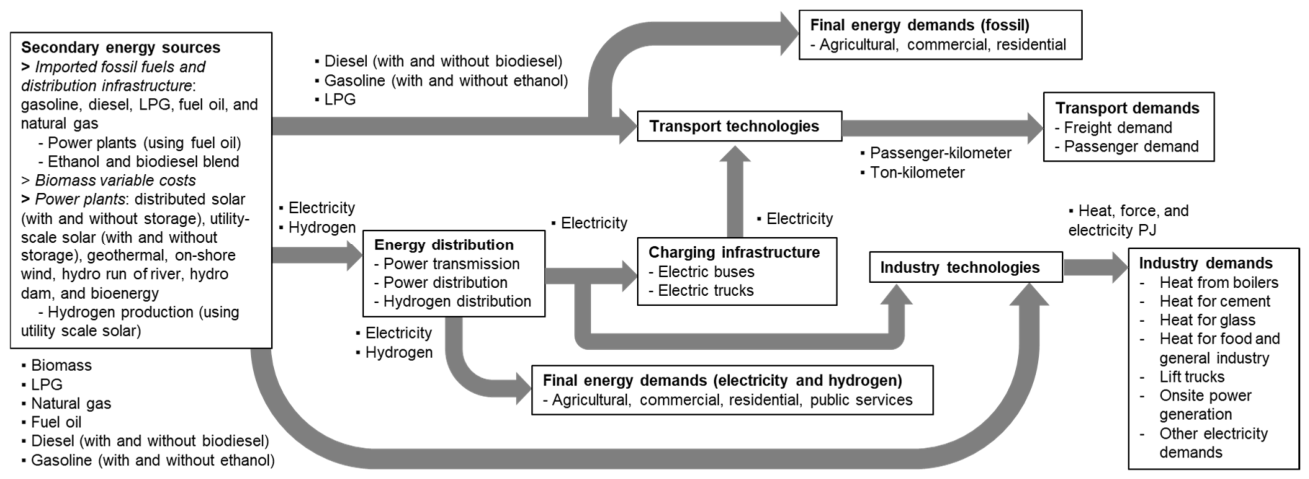
Figure 2.
The process to calculate the metrics of merit of every mitigation measure.
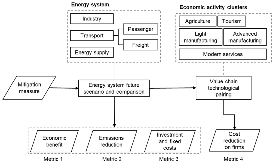
Figure 3.
Association between OSeMOSYS cost modeling and input-output matrix.
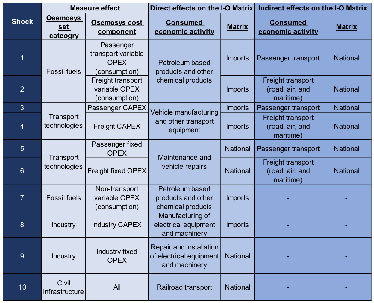
Figure 4.
Economic performance of the NDP scenario. a) Financial expenses per sector, b) Economic benefits per sector, c) Economic benefits per expense type.
Figure 4.
Economic performance of the NDP scenario. a) Financial expenses per sector, b) Economic benefits per sector, c) Economic benefits per expense type.
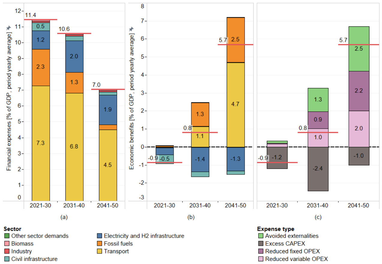
Figure 5.
Emissions of carbon dioxide equivalent (CO2e). a) for the BAU scenario by sector, b) for the NDP scenario by sector, c) for the NDP scenario by sector and fuel.
Figure 5.
Emissions of carbon dioxide equivalent (CO2e). a) for the BAU scenario by sector, b) for the NDP scenario by sector, c) for the NDP scenario by sector and fuel.
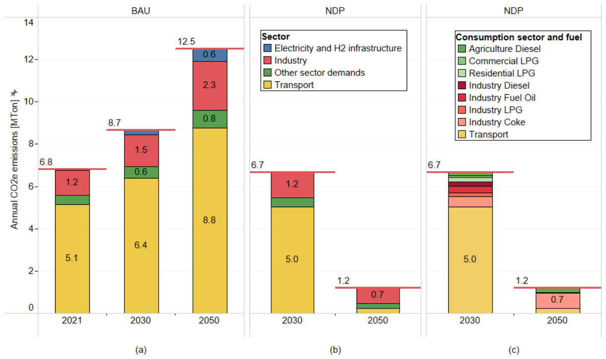
Figure 6.
Techno-economic performance for every measure group scenario with central ambition.
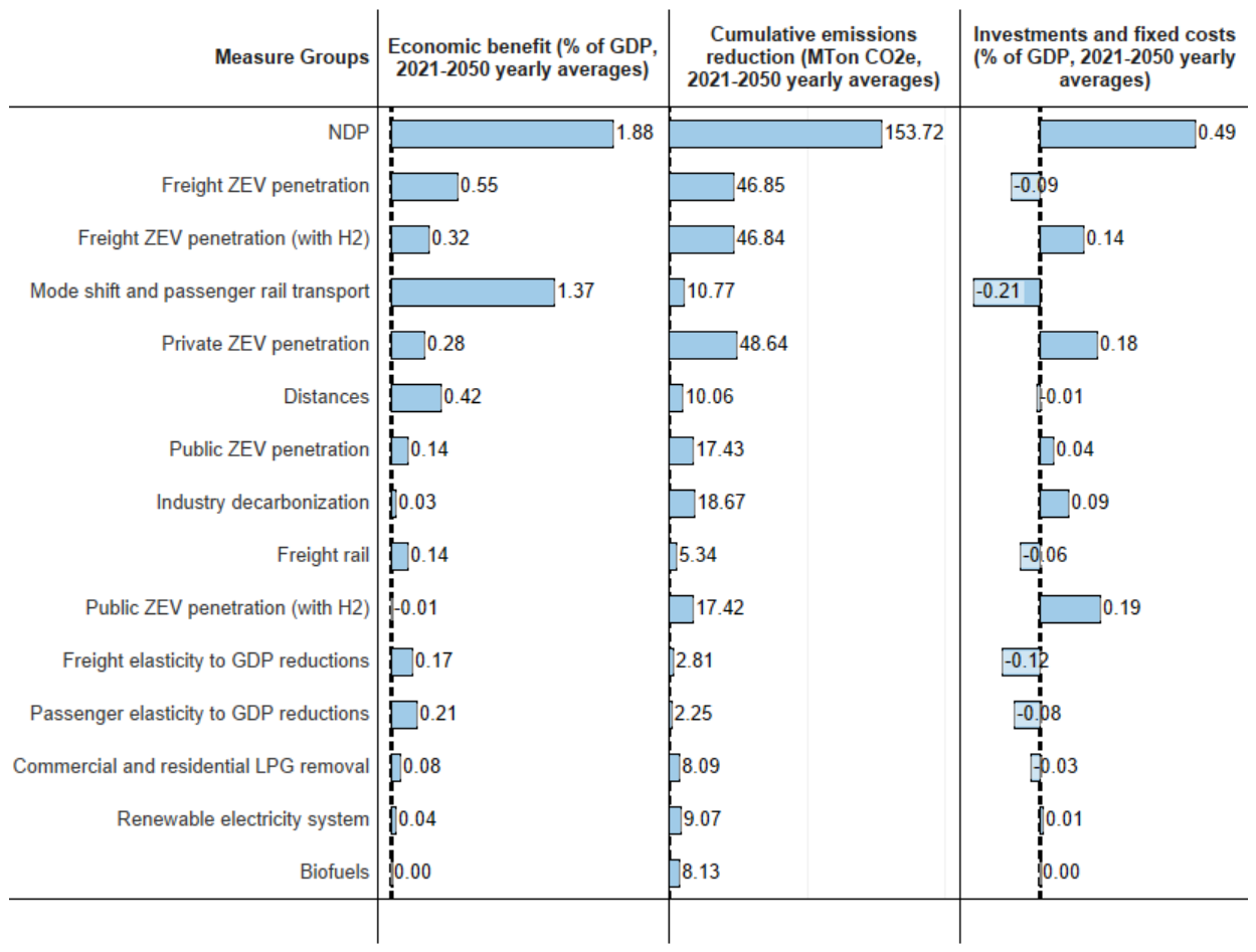
Figure 7.
Financial impacts by sector and measure group scenario (2021-2050% of GDP yearly average).
Figure 7.
Financial impacts by sector and measure group scenario (2021-2050% of GDP yearly average).
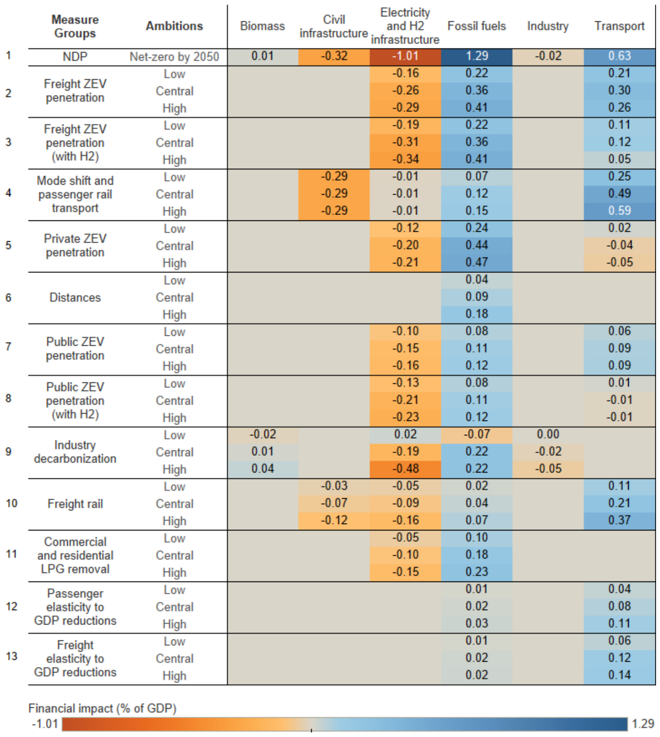
Figure 8.
Cost reduction by economic cluster a) for the NDP scenario and b) per measure group scenario. Values are 2021-2050 yearly averages.
Figure 8.
Cost reduction by economic cluster a) for the NDP scenario and b) per measure group scenario. Values are 2021-2050 yearly averages.
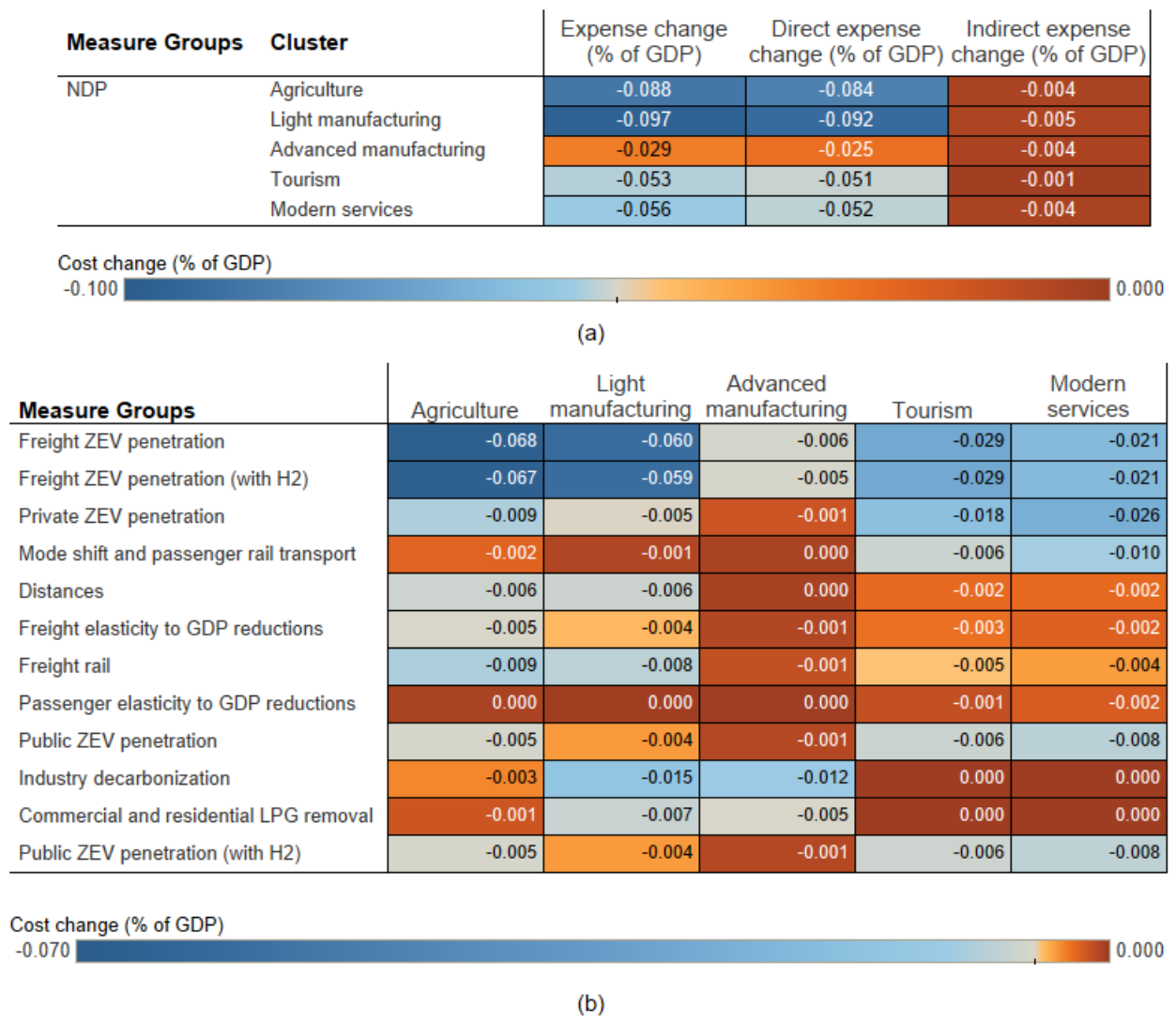
Figure 9.
Policy ranking by metric a) comparing the number of variables in the metric and b) comparing the ranking change.
Figure 9.
Policy ranking by metric a) comparing the number of variables in the metric and b) comparing the ranking change.
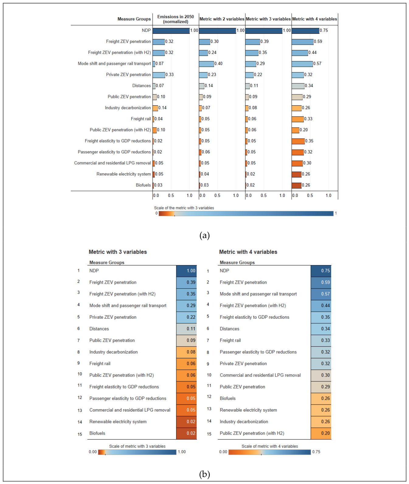
Figure 10.
Policy ranking by measure group and ambition with a metric with three variables (without considering the investment and fixed costs). The order is according to central ambition.
Figure 10.
Policy ranking by measure group and ambition with a metric with three variables (without considering the investment and fixed costs). The order is according to central ambition.
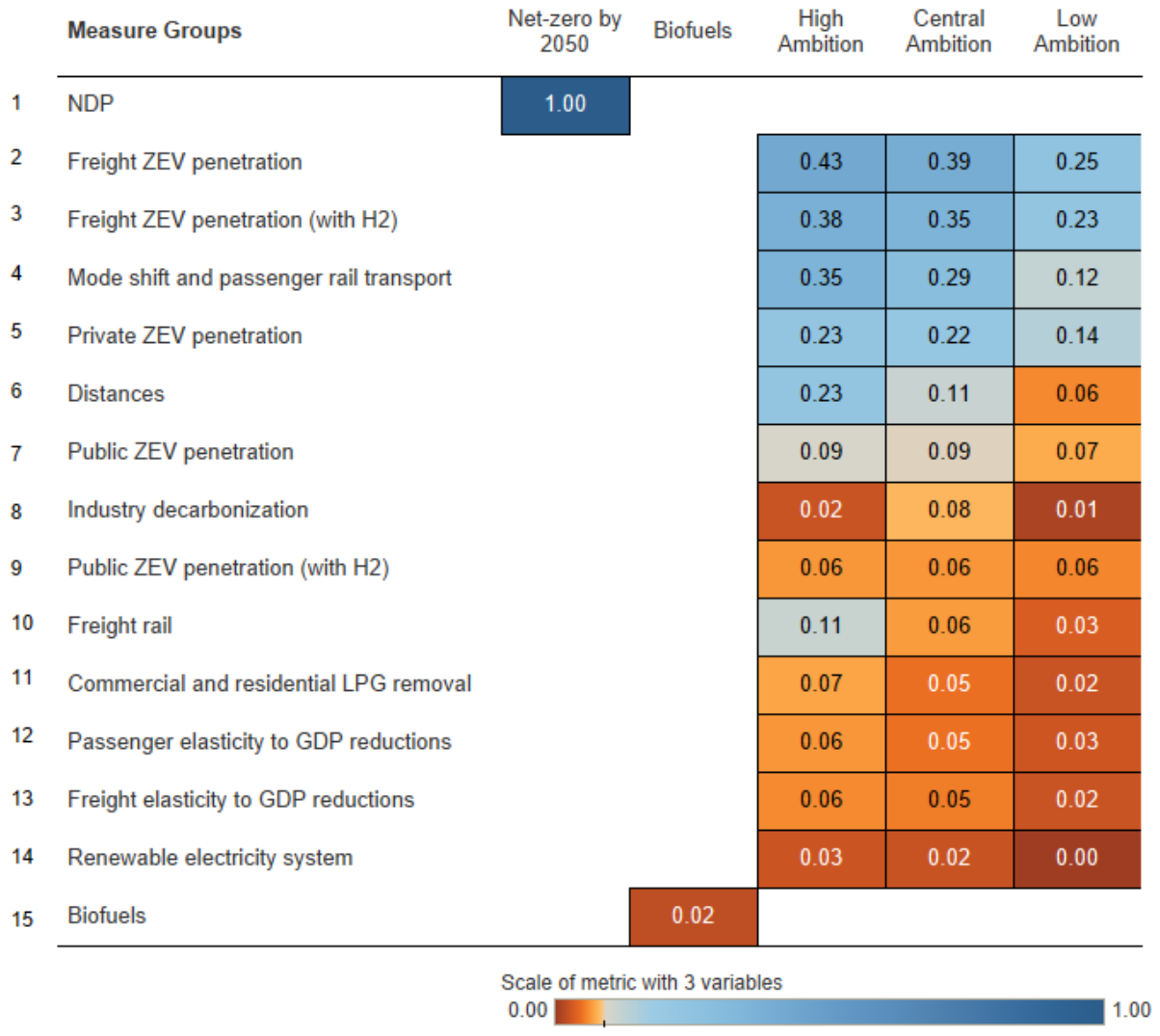
Figure 11.
Policy ranking by measure group and ambition with a metric with the four variables. The order is according to central ambition.
Figure 11.
Policy ranking by measure group and ambition with a metric with the four variables. The order is according to central ambition.
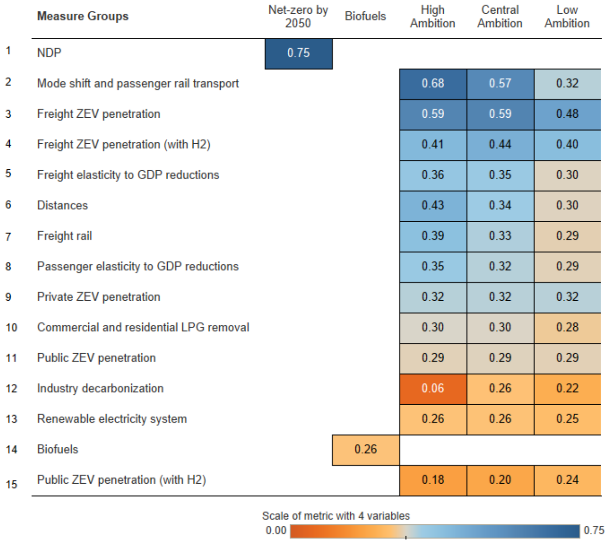
Table 1.
Economic activity clusters that increase Costa Rica’s economic complexity [56].
Table 1.
Economic activity clusters that increase Costa Rica’s economic complexity [56].
| Cluster | Subcluster | Economic activity |
|---|---|---|
| Agriculture | Agriculture (crop production) | Vegetables |
| Pineapple | ||
| Coffee | ||
| Fruits and nuts | ||
| Processing and conservation of fruits and vegetables | ||
| Fishing and aquaculture | Fishing | |
| Aquaculture | ||
| Forestry | Forestry and logging | |
| Light manufacturing | Cement, iron, and steel (fabrication) | Cement |
| Common metals | ||
| Metal-based products (except machinery) | ||
| Chemistry and extraction (fabrication or extraction) | The exploitation of other mines and quarries | |
| Paper | ||
| Petroleum-based products and other chemical products | ||
| Advanced manufacturing | Aerospace and high-technology | Electrical equipment and machinery |
| Vehicle and other transport equipment manufacturing | ||
| Biotechnology | Pharmaceutical products, medicinal chemicals, and botanical products | |
| Information and communication technologies | Electronic components, computers, and other peripheral equipment | |
| Electronic and optic products | ||
| Pharmaceutical and medical equipment | Medical and dental supplies | |
| Tourism | All | Accommodation |
| Food and beverages | ||
| Vehicle rentals | ||
| Travel agencies and related activities | ||
| Modern Services* | Knowledge economy | Programming and informatics |
| Legal activities | ||
| Accounting activities | ||
| Financial, human resources, and marketing consultancy | ||
| Architectural and engineering technical analysis | ||
| Scientific research and development | ||
| Other professional, scientific, and technical activities | ||
| Leasing of intellectual property | ||
| Administrative tasks and other support to firms | ||
| Orange economy | Movies, videos, television programs, music, etc | |
| Marketing | ||
| Creative, artistic, and entertainment | ||
| Libraries, museums, and other cultural activities | ||
| Sports and recreational activities | ||
| * Modern services also include renewable electricity production. | ||
Table 2.
Measures and interventions per parameter of the NDP scenario.
| Measure | Parameter | Intervention |
|---|---|---|
| Mode shift and passenger rail transport | Public passenger transport demand | Increase its participation in motorized transport by 7.5% in 2035 and 20% in 2050 |
| Non-motorized transport demand | It reduces motorized transport by 4% in 2035 and 10% in 2050 relative to BAU | |
| Electric passenger rail demand | Transports 0.1 Gpkm and enables public passenger transport mode shift | |
| Freight rail | Electric freight rail demand | Transport 10% of heavy freight demand in 2050, increasing linearly every year starting in 2024 |
| Heavy freight ZEV penetration | Fleet composition | 5% by 2030 and 50% by 2050 with electric and hydrogen technology |
| Light ZEV penetration | 5% by 2030 and 50% by 2050 with electric technology. By 2030, 20% of the fleet uses LPG, and the restriction is removed afterward | |
| Public ZEV penetration | 30% by 2035 and 85% by 2050 with electric technology. 3%by 2035 and 10% by 2050 with hydrogen buses and minibusses. | |
| Private ZEV penetration | 35% by 2035 and 99% by 2050 with electric technologies | |
| Biofuels | % of the fuel volume | Biodiesel: 1% by 2026 and 5% by 2030. Gasoline (ethanol): 8% by 2022. |
| Boilers in industry | thermal / electrical / mechanical kW composition | 40% of biomass and 60% electric |
| Heat production in industry | 90% by 2050 with electric technology and 10% with biomass | |
| Heat production for glass | 99% by 2050 with electric technology | |
| Lift trucks | Entirely with electric technology | |
| On-site power generation | 60% by 2050 in battery storage. The rest with biomass | |
| Power generation renewability | % of fossil fuel-based production | 0% by 2050 |
| Power generation characteristics | Considerations for model restrictions | Hydropower is not further developed. Only planned geothermal projects are simulated. It is assumed that wind and solar (with and without storage) supply the growth in demand, including transport electrification. |
| Commercial and residential LPG consumption | LPG substitution with electricity | The LPG phase-out occurs by 2050, gradually starting in 2024. The demand is substituted with electricity on a 1 to 1 basis. |
Table 3.
Description of energy sector mitigation measures by ambition level.
| Strategy ID | Measure Groups | NDC contribution | Lower ambition | Central ambition | Higher ambition |
|---|---|---|---|---|---|
| 1 | Biofuels | Biodiesel: 1% by 2026 and 5% by 2030. Gasoline: 8% by 2022. We do not consider relative cost differences between biofuels and fossil fuels. We consider a single level of ambition. | |||
| 2 | Mode shift and passenger rail transport | 1.1 | 35% of motorized passenger transport in 2050 | 50% of motorized passenger transport in 2050 | 50% of motorized passenger transport in 2040 |
| 1.5 | 5% of passenger transport in 2050 | 10% of passenger transport in 2050 | 10% of passenger transport in 2040 | ||
| 3 | Freight rail | 1.3 | 5% of heavy freight transport in 2050 | 20% of heavy freight transport in 2050 | 35% of heavy freight transport in 2050 |
| 4.a | Public ZEV penetration | 1.4 | 15% in 2035 and 50% in 2050 | 30% in 2035 and 85% in 2050 | 35% in 2035 and 100% in 2050 |
| 4.b | (include H2 for half of the participation) | ||||
| 5 | Private ZEV penetration | 1.6 and 1.7 | 15% in 2035 and 50% in 2050. | 30% in 2035 and 95% in 2050. | 35% in 2035 and 100% in 2050. |
| 6 | Passenger elasticity to GDP reductions | 1.8 | Decrease the demand elasticity to GDP by 10% in 2050 | Decrease the demand elasticity to GDP by 10% in 2030 | Decrease the demand elasticity to GDP by 25% in 2050 |
| 7 | Freight elasticity to GDP reductions | 1.9 | |||
| 8 | Distances | 2.2 | Apply 0.95 in 2050 to passenger and freight distances | Apply 0.9 in 2050 to passenger and freight distances | Apply 0.8 in 2050 to passenger and freight distances |
| 9 | Renewable electricity system | 3.1 | 98% renewable electricity production | Keeps 100% renewable electricity production by 2050 | Keeps 100% renewable electricity production by 2030 |
| 10 | Commercial and residential LPG removal | 3.2 | Keeps half the BAU’s LPG proportion | Removes LGP by 2050 | Removes LPG by 2030 |
| 11 | Industry decarbonization | 3.3 | Substitutes oil for natural gas and LPG by 2050 | Substitutes oil for biomass and electricity in 2050 | Substitutes oil for electricity and hydrogen in 2050 |
| 12.a | Freight ZEV penetration | 3.4 | 15% in 2035 and 50% in 2050 | 30% in 2035 and 85% in 2050 | 35% in 2035 and 100% in 2050 |
| 12.b | (include H2 for half of the participation) | ||||
| 13 | Electrical energy intensity reduction | 4.2 | Keeps energy intensity as in 2018 | Decrease energy intensity 25% in 2050 relative to 2018 | Decrease energy intensity in 2050 35% relative to 2018 |
| 14 | Renewable options analyses | 4.4 | Prefers predominant hydro and geothermal | Keeps hydro and geothermal, adds more wind and utility solar | Distributed solar with storage rises significantly. |
Table 4.
Techno-economic performance of special benchmark scenarios.
| Measure groups | Ambition | Economic benefit (% of GDP 1) | Avoided emissions (MTon of CO2e) | Cost change on electricity and H2 infrastructure (% of GDP 1) | Cost change on fossil fuels (% of GDP 1) |
|---|---|---|---|---|---|
| Renewable electricity system | Central | 0.037 | -9.1 | -0.02 | 0.06 |
| High | 0.04 | -9.9 | -0.02 | 0.06 | |
| Renewable options analyses | Low | -0.343 | not compared | -0.34 | 0.06 |
| High | 0.04 | not compared | 0.04 | 0.06 | |
| Electrical energy intensity reduction | Low | -0.18 | not compared | -0.18 | |
| High | 0.054 | not compared | 0.05 |
1% of GDP results are yearly averages between 2021 and 2050.
Disclaimer/Publisher’s Note: The statements, opinions and data contained in all publications are solely those of the individual author(s) and contributor(s) and not of MDPI and/or the editor(s). MDPI and/or the editor(s) disclaim responsibility for any injury to people or property resulting from any ideas, methods, instructions or products referred to in the content. |
© 2026 by the authors. Licensee MDPI, Basel, Switzerland. This article is an open access article distributed under the terms and conditions of the Creative Commons Attribution (CC BY) license (http://creativecommons.org/licenses/by/4.0/).
Copyright: This open access article is published under a Creative Commons CC BY 4.0 license, which permit the free download, distribution, and reuse, provided that the author and preprint are cited in any reuse.


