

Submitted:
02 July 2026
Posted:
07 July 2026
You are already at the latest version
Abstract
With the rapid proliferation of the Internet of Things (IoT) and edge computing, there is a growing demand for efficient, on-device learning algorithms that can operate under strict power, memory, and latency constraints. The Forward Forward (FF) algorithm has emerged as a biologically plausible alternative to backpropagation, offering local learning rules that avoid global error propagation. Recently, Self-Contrastive Forward-Forward (SCFF) learning was proposed to combine FF with contrastive self-supervised learning, enabling unsupervised representation learning. It currently achieves the highest recognition accuracy among unsupervised local learning algorithms. However, its original convolutional pipeline suffers from redundant feature extraction and potential distribution mismatches in negative sample processing. These limitations lead to high computational overhead and restrict the model’s scalability on resource-constrained devices. Therefore, Self-Contrastive Single Forward (SCSF) is proposed to address these computational bottlenecks and distribution inconsistencies. The key idea is to move the self-contrastive construction from the raw-input domain to the feature domain, thereby reusing shared features for both positive and negative sample construction. Extensive experiments on CIFAR-10, STL-10, and Tiny-Imagenet demonstrate that SCSF maintains competitive recognition accuracy with slight improvements, while significantly boosting computational efficiency. Efficiency benchmarks on the training forward pass show that SCSF reduces Giga Floating Point Operations Per Second (GFLOPS) by 75% and improves throughput by an average of 3.00× across different input resolutions. These results confirm that SCSF significantly boosts computational efficiency while preserving unsupervised representation performance, making it a promising candidate for real-time, unsupervised representation learning on edge devices and neuromorphic hardware.
Keywords:
forward-forward algorithm
; self-contrastive learning
; local learning
; unsupervised learning
; edge computing
1. Introduction
FF provides an alternative learning paradigm to conventional end-to-end backpropagation by optimizing layer-wise goodness objectives through forward-only computation [1]. Based on this paradigm, SCFF extends FF to unsupervised representation learning by constructing positive and negative sample pairs from unlabeled data [2]. It currently stands as one of the state-of-the-art methods in unsupervised local learning, achieving the highest recognition accuracy among its peers. These algorithms are particularly relevant to on-device and edge-side learning, where privacy, latency, memory, and energy constraints require training algorithms that are computationally efficient and hardware-compatible [3,4].
Traditional deep neural networks are usually trained by backpropagation [5]. Although backpropagation has achieved remarkable success in a wide range of machine learning tasks, it relies on global error propagation, forward-backward computation, and the storage of intermediate activations. These requirements make it expensive for edge devices with limited computing and memory resources, especially for learning-in-memory and crossbar-array-based hardware systems [6]. In addition, the backward pass introduces non-local dependencies between layers, which makes direct hardware implementation more complicated.
Local learning algorithms provide a promising alternative by reducing or eliminating global dependency during training. Since each layer can be optimized using local information, local learning is attractive for hardware-friendly and biologically inspired computation, especially in neuromorphic computing systems [7]. Among existing local learning algorithms, FF-based algorithms are especially attractive because they preserve a forward-only computational structure during both inference and learning. This property makes them potentially suitable for resource-constrained edge devices, where bidirectional signal propagation, large activation buffers, and complex backward circuits are difficult to support.
SCFF is conceptually related to contrastive self-supervised learning, where positive and negative pairs are constructed to learn discriminative representations from unlabeled data [8,9]. However, unlike conventional contrastive learning algorithms that usually rely on global representation comparison, projection heads, strong data augmentation, or large numbers of negative pairs, SCFF incorporates positive-negative construction into the FF-style layer-wise goodness optimization framework. Specifically, SCFF constructs positive samples by pairing an image with itself and negative samples by pairing different images. This self-contrastive mechanism enables FF-style networks to learn useful representations without explicit labels and significantly improves the unsupervised learning ability of the original FF algorithm.
Despite its advantages, SCFF still has two important limitations that restrict its practical efficiency and representation quality.
First, SCFF introduces redundant convolutional computation. In its core feature extraction stage, positive and negative branches are processed separately. Since positive and negative pairs are formed by reusing images from the same mini-batch, many convolutional operations are repeated on identical or highly overlapping image tensors. This repeated computation increases training and inference latency, making SCFF less suitable for low-power edge devices.
Second, the preprocessing order of SCFF may distort the distribution of negative samples. In the original pipeline, positive and negative image pairs are first concatenated and normalized as combined tensors. They are then split into sub-samples and fed into convolutional layers. Although the concatenated tensor can be normalized to have approximately zero mean and unit variance, the two split components may no longer individually follow the desired normalized distribution, especially for negative pairs composed of two different images. This problem weakens the statistical consistency between positive and negative branches and may reduce the effectiveness of goodness-based optimization.
To address these problems, this paper proposes the Self-Contrastive Single-Forward algorithm. The key idea is to move self-contrastive construction from the raw-input domain to the feature domain. Specifically, SCSF first preprocesses the original image batch, then performs only one convolutional forward pass to obtain shared feature maps, and finally constructs positive and negative feature samples through feature addition and batch-wise cyclic shifting. Compared with SCFF, SCSF eliminates redundant repeated convolution while preserving the self-contrastive learning principle.
The main contributions of this work are summarized as follows:
- Single-forward self-contrastive feature extraction: We redesign the SCFF computational pipeline and reduce the number of convolutional operations in the core self-contrastive stage from four to one. This significantly reduces computational cost and improves throughput.
- Distribution-preserving preprocessing strategy: Instead of normalizing concatenated positive and negative pairs, SCSF normalizes original individual samples before convolution. This avoids the distribution mismatch caused by splitting normalized concatenated negative pairs.
- Feature-domain positive and negative construction: SCSF constructs positive and negative samples directly from shared feature maps. Positive samples are constructed by combining a feature map with itself, while negative samples are constructed by combining feature maps from different images using cyclic batch shifting.
- Comprehensive experimental validation: Experiments on CIFAR-10, STL-10, and Tiny ImageNet demonstrate that SCSF maintains or slightly improves the accuracy of SCFF while achieving substantial computational acceleration.
The remainder of this paper is organized as follows. Section II reviews related work on local learning and FF-based algorithms. Section III introduces the proposed SCSF algorithm in detail. Section IV presents experimental settings and results. Section V concludes the paper and outlines future research directions.
2. Related Works
2.1. Local Learning for Edge Computing
Local learning algorithms aim to reduce or eliminate global dependency during training. Unlike conventional backpropagation, where weight updates depend on error signals propagated from the output layer to earlier layers, local learning algorithms update parameters using local signals available at each layer or module. This property makes them attractive for edge computing and neuromorphic hardware.
Hebbian learning is one of the earliest and most representative local learning principles[10]. It updates synaptic weights according to correlations between pre-synaptic and post-synaptic activities. Modern Hebbian variants, such as HardHebb and SoftHebb, combine Hebbian-style updates with deep neural architectures and have shown promising performance on image classification datasets[11,12,13]. Other Hebbian algorithms include Hebb-CHU and Hebb-PNorm[14,15]. However, their practical performance often depends on carefully designed normalization strategies, competition mechanisms, or special activation functions.
Energy-based local learning algorithms, such as Equilibrium Propagation, train networks by minimizing energy functions[16,17,18]. DualProp further improves energy-based local learning[19]. These algorithms can approximate gradient-based learning under certain conditions and have achieved competitive performance. Nevertheless, many energy-based algorithms require iterative relaxation toward equilibrium states and may involve bidirectional connections or multiple inference phases, which can increase implementation complexity in hardware-oriented scenarios.
Feedback alignment and direct feedback alignment simplify backpropagation by replacing exact backward weights with random feedback matrices[20,21]. These algorithms reduce the biological implausibility of exact weight transport, but they still rely on feedback or backward-like error signals, which makes them different from strictly forward-only learning paradigms.
Compared with these algorithms, FF-based learning provides a distinctive forward-only training paradigm. It optimizes each layer independently by separating positive and negative samples according to a local goodness score. This property gives FF-based algorithms potential advantages in hardware implementation and edge-side learning.
2.2. Forward-Forward Algorithm
The Forward-Forward algorithm replaces the forward-backward training process of backpropagation with two forward passes: one for positive samples and one for negative samples[1]. Each layer computes a scalar goodness score, commonly defined as the sum or average of squared neural activations. The training objective encourages positive samples to produce goodness values above a threshold and negative samples to produce goodness values below a threshold. Formally, given a layer output vector y, the goodness can be written as
where M is the number of neurons or activation elements. A logistic loss is then applied to separate positive and negative samples. Since the loss is defined locally for each layer, the update of one layer does not require gradients propagated through all subsequent layers. This property distinguishes FF from standard backpropagation.
However, the original FF algorithm requires an effective mechanism to construct positive and negative samples. In supervised learning, labels can be embedded into inputs to construct positive and negative examples. In unsupervised learning, however, constructing meaningful negative samples is more challenging[22,23].
2.3. Self-Contrastive Forward-Forward Algorithm
The Self-Contrastive Forward-Forward algorithm addresses the above issue by introducing a self-contrastive strategy. It constructs positive and negative pairs from unlabeled images [2]. A positive pair is formed by concatenating two identical images, while a negative pair is formed by concatenating two different images. The network is then trained to assign higher goodness scores to positive pairs and lower goodness scores to negative pairs.
This design allows FF-based networks to learn representations without labels. Nevertheless, the original SCFF pipeline contains repeated convolutional computation and a potentially problematic preprocessing order.
As shown in Figure 1(a), the original SCFF procedure can be summarized as follows:
- Pair construction: Positive pairs are constructed as , while negative pairs are constructed as , where .
- Pair-level normalization: The concatenated positive and negative pairs are normalized as complete tensors.
- Splitting and convolution: The normalized pairs are split into sub-samples. Separate convolution operations are then performed for the positive and negative branches.
- Goodness computation: The goodness scores of positive and negative branches are computed and optimized using the FF loss.
Although effective, this process has two drawbacks. First, convolution is repeatedly applied to images that are already present in the same mini-batch. Second, pair-level normalization may not guarantee that each split component remains individually normalized, especially for negative pairs formed from different images. These two issues motivate the proposed SCSF algorithm.
3. Proposed Methods
3.1. Overview
The proposed SCSF algorithm redesigns the SCFF pipeline from an input-pair-based computation process to a shared-feature-based computation process. The central principle is to normalize each original sample first, extract its feature map once, and then construct positive and negative feature samples in the feature domain. The motivation behind this redesign comes from two observations.
First, the self-contrastive relationship used in SCFF does not necessarily have to be constructed in the raw-input domain. The essential idea of SCFF is to compare self-consistent pairs with inconsistent pairs. In the original implementation, this comparison is performed by concatenating images before convolution. However, convolutional layers are designed to extract local visual patterns and intermediate representations from images. Therefore, self-consistency and cross-sample inconsistency can also be represented after feature extraction. In SCSF, the positive feature sample strengthens the response of the same image feature, while the negative feature sample combines feature maps from different images. The goodness objective can still learn to separate these two types of feature combinations, which preserves the self-contrastive learning signal while avoiding redundant input-domain convolution.
Second, goodness-based learning is sensitive to activation magnitude because the goodness score is directly computed from squared activations. If positive and negative branches are generated from statistically inconsistent inputs, the model may partially rely on distribution artifacts rather than meaningful structural differences. In SCFF, pair-level normalization can normalize the concatenated pair as a whole, but the split sub-samples may not individually remain normalized, especially for negative pairs composed of two different images. SCSF avoids this problem by normalizing original samples before convolution. Consequently, both positive and negative feature samples are constructed from normalized and statistically consistent feature representations.
As shown in Figure 1(b), the overall SCSF pipeline consists of four stages:
- Original sample preprocessing
- Single convolutional forward pass
- Feature-domain positive and negative construction
- local goodness computation and layer-wise optimization
Compared with SCFF, SCSF does not change the basic FF learning objective [1,2]. Instead, it changes the order and location of preprocessing, convolution, and positive/negative sample construction. This design reduces repeated convolution, preserves the self-contrastive learning principle, and improves the statistical consistency of inputs used for goodness-based optimization.
3.2. Original Sample Preprocessing
Let a mini-batch of input images be denoted as
where b is the batch size. In SCFF, positive and negative pairs are constructed before normalization. In contrast, SCSF directly preprocesses the original image batch.
The preprocessing operation can include padding, resizing, dataset-level normalization, and batch-wise standardization depending on the dataset and implementation; such normalization techniques are widely used to stabilize deep neural network training[24]. In our implementation, the same basic preprocessing settings as SCFF are retained for fair comparison, except that the normalization operation is performed before positive and negative construction.
For each image , the normalized input is
where and denote the mean and standard deviation used for normalization, and is a small constant for numerical stability.
As illustrated in Figure 2(a), the original SCFF procedure applies normalization to the concatenated tensor. While this normalizes the pair as a whole, splitting the tensor—especially for negative pairs composed of two distinct images—often results in sub-samples that no longer individually follow the desired normalized distribution. This distribution mismatch may cause the model to rely on statistical artifacts rather than semantic features.
In contrast, Figure 2(b) demonstrates the SCSF strategy. By normalizing the original individual samples before concatenation, we ensure that both positive and negative branches maintain a consistent distribution throughout the network, which is crucial for stable hardware-friendly learning.
This preprocessing order provides normalized individual inputs for the subsequent shared convolutional pass, which is essential for constructing positive and negative feature samples from a consistent feature distribution.
3.3. Single Convolutional Forward Pass
After preprocessing, SCSF applies one convolutional forward pass to the normalized mini-batch:
where denotes the convolutional transformation of layer l, and is the feature map of the i-th sample.
In the original SCFF pipeline, multiple convolution operations are required to process the two components of positive and negative pairs. Since these components are repeatedly drawn from the same original mini-batch, redundant feature extraction occurs.
SCSF avoids this redundancy by computing each sample feature only once. The obtained feature maps are then reused for both positive and negative construction. This reduces the main convolutional computation by approximately 75% in the core stage, since the number of convolution operations is reduced from four to one.
This single-forward design also reduces repeated memory access and simplifies the computation graph. Although the effect of floating-point rounding error is usually small in modern GPU computation, avoiding repeated convolution can still improve numerical consistency and reduce unnecessary accumulation of minor numerical deviations.
3.4. Feature-Domain Positive and Negative Construction
After obtaining shared feature maps, SCSF constructs positive and negative samples directly in the feature domain.
Let denote the feature map of the i-th sample in the mini-batch. The positive feature sample is constructed by combining the feature map with itself:
The negative feature sample is constructed by combining with another feature map selected through cyclic shifting:
where m is a fixed shift step and b is the batch size. To ensure that negative pairs are formed from different samples, m should satisfy
In practice, m can be set to , a fixed non-zero integer, or randomly sampled at each iteration. A fixed cyclic shift is simple and efficient, while random shifting can increase negative-pair diversity.
The feature-domain construction preserves the self-contrastive idea of SCFF. Positive samples still represent self-consistency, while negative samples represent inconsistency between different images. However, SCSF constructs these samples after convolution rather than before convolution, thereby avoiding repeated feature extraction.
3.5. Goodness Computation
For each layer, SCSF uses the same type of goodness function as FF and SCFF[1,2]. Given the activation output of layer l, the goodness score is defined as the average squared activation:
where denotes the total number of activation elements in layer l, and denotes the m-th activation element.
For positive and negative feature samples, the corresponding goodness scores are denoted as and The learning objective is to make positive samples obtain goodness values higher than a predefined threshold and negative samples obtain goodness values lower than the threshold.
3.6. Local Loss Function
Following FF and SCFF, for each layer l, SCSF adopts a logistic goodness loss[1,2]. The probability that a positive sample is recognized as positive is defined as
and the probability that a negative sample is recognized as negative is defined as
where is the sigmoid function and is the layer-wise goodness threshold. The local loss of layer l is written as
This loss encourages positive samples to move above the threshold and negative samples to move below the threshold. It should be emphasized that SCSF does not require end-to-end backpropagation across the whole network. Each layer is optimized using its own local loss. In implementation, gradients may still be computed locally within a layer by automatic differentiation, but no global error signal needs to be propagated from the final classifier to all earlier layers. This maintains the local learning property of FF-based algorithms.
4. Experiments
4.1. Datasets
We evaluate the proposed SCSF algorithm on three commonly used image classification datasets with different levels of complexity.
- CIFAR-10: CIFAR-10 contains 60 000 colour images of size , divided into 10 classes. There are 50,000 training images and 10 000 test images[25].
- STL-10: STL-10 contains colour images with higher resolution and fewer labeled samples. It is more challenging than CIFAR-10 due to larger image size and stronger intra-class variations[26].
- Tiny ImageNet: Tiny ImageNet contains 200 classes and images resized to . It is significantly more complex than CIFAR-10 and STL-10 due to the larger number of categories and more diverse visual patterns[27].
These datasets are selected to evaluate both the representation ability and scalability of SCSF.
4.2. Implementation Details
For fair comparison, SCSF follows the same network architecture and training protocol as the SCFF baseline unless otherwise specified[2]. The main difference lies in the preprocessing and self-contrastive construction pipeline.
All experiments in the ablation study are conducted under the same hardware environment using an NVIDIA RTX 4060 GPU with 8 GB memory. The same random seed setting, optimizer type, batch size, and training epochs are used for SCFF, SCFF-PostNorm, and SCSF to reduce the influence of implementation differences.
The reported accuracy is top-1 classification accuracy. For efficiency evaluation, we measure GFLOPs and FPS strictly during the training forward pass. We evaluate a single convolutional layer using input tensors sized to match the three target datasets: 1×3×32×32 for CIFAR-10, 1×3×48×48 for STL-10, and 1×3×64×64 for Tiny-Imagenet. This layer-level setup isolates the architectural computational overhead and ensures a consistent, fair comparison across different spatial resolutions.
4.3. Comparison with Related Algorithms
Table 1 compares SCSF with representative learning algorithms that are commonly discussed as alternatives or complements to conventional end-to-end backpropagation, including Hebbian learning, feedback-alignment-based learning, energy-based learning, forward-only learning, and local self-supervised learning algorithms.
From Table 1, it can be observed that SCSF achieves competitive performance among unsupervised local learning and FF-based algorithms. Compared with the original SCFF baseline, SCSF maintains the same accuracy on CIFAR-10 and slightly improves the accuracy on STL-10 and Tiny ImageNet. Specifically, using the one-decimal reporting format in Table I, SCSF achieves 80.8% on CIFAR-10, 77.4% on STL-10, and 35.9% on Tiny ImageNet, compared with 80.8%, 77.3%, and 35.7% obtained by SCFF. These results indicate that the proposed pipeline optimization improves computational efficiency without sacrificing recognition performance.
It should be noted that several supervised algorithms, such as SigProp and DualProp, report higher CIFAR-10 accuracy. However, these algorithms are not unsupervised according to the comparison setting in Table I. In contrast, SCSF learns representations from unlabeled data and preserves the FF-style local goodness optimization mechanism. Therefore, the main advantage of SCSF is not to surpass all supervised alternatives in classification accuracy, but to improve the efficiency of SCFF while maintaining competitive unsupervised representation learning performance.
4.4. Ablation Study
To analyze the contribution of each component, we conduct an ablation study with three variants. Unlike the one-decimal results reported in the overall comparison in Table I, the ablation study reports reproduced results with two decimal places under our unified hardware and software environment. This reporting format is used to make small but consistent performance differences between model variants visible, which would otherwise be hidden by one-decimal rounding.
- SCFF: The original baseline using concatenation-first normalization and four convolutional forward computations.
- SCFF-PostNorm: An intermediate variant that keeps the four-convolution structure but changes the normalization order. Instead of normalizing concatenated pairs before splitting, it normalizes samples after splitting. This variant is used to isolate the effect of distribution correction.
- SCSF: The complete proposed method using both distribution-preserving preprocessing and single-forward feature-domain construction.

Table 2.
Ablation study on core improvements (%).
| Algorithm | CIFAR-10 | STL-10 | Tiny-ImageNet |
|---|---|---|---|
| SCFF | 80.58 | 76.68 | 35.20 |
| SCFF-PostNorm | 80.62 | 76.71 | 35.74 |
| SCSF (Ours) | 80.77 | 77.40 | 35.91 |
The results show a clear performance order: Compared with SCFF, SCFF-PostNorm obtains consistent improvements on all datasets. This indicates that the normalization order in the original SCFF pipeline indeed affects training performance. In particular, the improvement on Tiny ImageNet is more visible, which suggests that distribution inconsistency becomes more influential as dataset complexity increases.
SCSF further improves performance over SCFF-PostNorm. This demonstrates that the single-forward feature-domain design does not merely reduce computation, but also preserves or improves representation quality. The improvement may come from two aspects. First, shared feature extraction ensures that positive and negative samples are constructed from a consistent feature space. Second, the removal of repeated convolution reduces unnecessary numerical and computational variation.
Overall, the ablation results confirm that both distribution-preserving preprocessing and single-forward feature reuse are useful for improving SCFF.
4.5. Computational Efficiency Evaluation
To evaluate computational efficiency, we compare GFLOPs and FPS between SCFF and SCSF using the same convolutional layer and input size.
To evaluate efficiency gains, we compare the training forward-pass cost and throughput of SCSF against SCFF across the three resolutions defined in the implementation details. Figure 3 presents the GFLOPS comparison. By sharing feature extraction across branches, SCSF reduces the training forward-pass FLOPS by approximately 75% at all tested resolutions. For example, at the STL-10 resolution, the cost drops from 0.265 to 0.066 GFLOPS.
Figure 4 illustrates the corresponding throughput (FPS). SCSF consistently achieves a processing speed 3.00× higher than SCFF on average (3.05× for CIFAR-10, 2.97× for STL-10, and 2.97× for Tiny-Imagenet). This sustained acceleration confirms that the single-forward design effectively eliminates redundant convolutions, making SCSF highly suitable for latency-constrained edge training.
Nevertheless, the efficiency gain is significant. Since convolution is usually the dominant operation in CNN-based models, reducing repeated convolution directly benefits edge deployment. The proposed method is therefore suitable for scenarios where power consumption, latency, and computational resources are strictly limited.
5. Conclusion
In this paper, we proposed the Self-Contrastive Single-Forward algorithm. The proposed method addresses two limitations of SCFF: redundant repeated convolution and negative sample distribution distortion caused by concatenation-first normalization.
SCSF first normalizes original individual samples, then extracts shared feature maps through a single convolutional forward pass, and finally constructs positive and negative samples directly in the feature domain. This design reduces the number of convolutional operations in the core self-contrastive stage from four to one, while preserving the layer-wise local optimization mechanism of FF-based learning.
Experimental results on CIFAR-10, STL-10, and Tiny ImageNet demonstrate that SCSF consistently outperforms SCFF under the same experimental setting. More importantly, computational benchmarks across varying input resolutions show that SCSF reduces training forward-pass FLOPS by approximately 75% and improves throughput by an average of 3.00× . These gains, achieved while maintaining high recognition accuracy, position SCSF as an accuracy-preserving, highly efficient backbone for future edge-AI and neuromorphic vision systems.
References
- Hinton, G. The forward-forward algorithm: some preliminary investigations. arXiv 2022, arXiv:2212.13345. [Google Scholar]
- Chen, X.; Liu, D.; Laydevant, J.; et al. Self-Contrastive Forward-Forward algorithm. Nat. Commun. 2025, 16, 5978. [Google Scholar] [CrossRef] [PubMed]
- Shi, W.; Cao, J.; Zhang, Q.; et al. Edge computing: vision and challenges. IEEE Internet Things J. 2016, 3(5), 637–46. [Google Scholar] [CrossRef]
- Khouas, A. R.; Bouadjenek, M. R.; Hacid, H.; et al. Training machine learning models at the edge: a survey. arXiv 2024, arXiv:2403.02619. [Google Scholar]
- Rumelhart, D. E.; Hinton, G. E.; Williams, R. J. Learning representations by back-propagating errors. Nature 1986, 323, 533–6. [Google Scholar] [CrossRef]
- Wang, W.; Li, Y.; Wang, M. Difficulties and approaches in enabling learning-in-memory using crossbar arrays of memristors. Neuromorphic Comput Eng. 2024, 4(3), 032002. [Google Scholar] [CrossRef]
- Marković, D.; Mizrahi, A.; Querlioz, D.; et al. Physics for neuromorphic computing. Nat. Rev. Phys. 2020, 2, 499–510. [Google Scholar] [CrossRef]
- Chen, T.; Kornblith, S.; Norouzi, M.; et al. A simple framework for contrastive learning of visual representations. Proc Int Conf Mach Learn, 2020; pp. 1597–607. [Google Scholar] [CrossRef]
- He, K.; Fan, H.; Wu, Y.; et al. Momentum contrast for unsupervised visual representation learning. Proc. IEEE Conf. Comput Vis. Pattern Recognit. 2020, 9729–38. [Google Scholar] [CrossRef]
- Hebb, D. O. The Organization of Behavior: A Neuropsychological Theory; Psychology Press: New York, NY, 2005. [Google Scholar]
- Miconi, T. Hebbian learning with gradients: Hebbian convolutional neural networks with modern deep learning frameworks. arXiv 2021, arXiv:2107.01729. [Google Scholar]
- Lagani, G.; Falchi, F.; Gennaro, C.; et al. Hebbian semi-supervised learning in a sample efficiency setting. Neural Netw. 2021, 143, 719–31. [Google Scholar] [CrossRef] [PubMed]
- Journé, A.; Rodriguez, H. G.; Guo, Q.; et al. Hebbian deep learning without feedback. Proc Int Conf Learn Represent, 2023. [Google Scholar]
- Krotov, D.; Hopfield, J. J. Unsupervised learning by competing hidden units. Proc. Natl. Acad. Sci. USA 2019, 116(16), 7723–31. [Google Scholar] [CrossRef]
- Grinberg, L.; Hopfield, J.; Krotov, D. Local unsupervised learning for image analysis. Proc NeurIPS Neuro AI Workshop, 2019. [Google Scholar]
- Scellier, B.; Bengio, Y. Equilibrium propagation: bridging the gap between energy-based models and backpropagation. Front Comput Neurosci. 2017, 11, 24. [Google Scholar] [CrossRef] [PubMed]
- Laborieux, A.; Ernoult, M.; Scellier, B.; et al. Scaling equilibrium propagation to deep convnets by drastically reducing its gradient bias. Front Neurosci. 2021, 15, 633674. [Google Scholar] [CrossRef] [PubMed]
- Liu, D.; Laydevant, J.; Pontlevy, A.; et al. Unsupervised end-to-end training with a self-defined target. Neuromorphic Comput Eng. 2024, 4(4), 044005. [Google Scholar] [CrossRef]
- Høier, R.; Staudt, D.; Zach, C. Dual propagation: accelerating contrastive Hebbian learning with dyadic neurons. Proc Int Conf Mach Learn, 2023; pp. 13141–56. [Google Scholar] [CrossRef]
- Nøkland, A. Direct feedback alignment provides learning in deep neural networks. Adv. Neural Inf. Process Syst. 2016, 29, 1–9. [Google Scholar] [CrossRef]
- Launay, J.; Poli, I.; Boniface, F.; et al. Direct feedback alignment scales to modern deep learning tasks and architectures. Adv. Neural Inf. Process Syst. 2020, 33, 1–12. [Google Scholar] [CrossRef]
- Wu, Y.; et al. Distance-forward learning: enhancing the forward-forward algorithm towards high-performance on-chip learning. arXiv 2024, arXiv:2408.14925. [Google Scholar]
- De Vita, F.; et al. μ-FF: on-device forward-forward training algorithm for microcontrollers. Proc IEEE Int Conf Smart Comput, 2023; pp. 49–56. [Google Scholar] [CrossRef]
- Huang, L.; et al. Normalization techniques in training DNNs: methodology, analysis and application. IEEE Trans. Pattern Anal. Mach. Intell. 2023, 45(8), 10173–86. [Google Scholar] [CrossRef]
- Krizhevsky, A.; Nair, V.; Hinton, G. CIFAR-10: Canadian Institute for Advanced Research. 14 June 2026. Available online: http://www.cs.toronto.edu/.
- Coates, A.; Ng, A.; Lee, H. An analysis of single-layer networks in unsupervised feature learning. Proc Int Conf Artif Intell Stat, 2011; pp. 215–23. [Google Scholar] [CrossRef]
- Le, Y.; Yang, X. Tiny ImageNet visual recognition challenge. CS 231N 2015, 7, 3. [Google Scholar]
- Kohan, A.; Rietman, E. A.; Siegelmann, H. T. Signal propagation: the framework for learning in a forward pass. IEEE Trans. Neural Netw. Learn Syst. 2024, 35(6), 8585–96. [Google Scholar] [CrossRef]
- Srinivasan, R. F.; et al. Forward learning with top-down feedback: empirical and analytical characterization. Proc Int Conf Learn Represent, 2024. [Google Scholar]
- Zhou, H. Activation learning by local competitions. arXiv 2022, arXiv:2209.13400. [Google Scholar]
- Webster, M. B.; Choi, J.; Ahn, C. Learning the connections in direct feedback alignment. 14 June 2026. Available online: https://openreview.net/forum?id=zgGmAx9ZcY.
- Tang, M.; Yang, Y.; Amit, Y. Biologically plausible training mechanisms for self-supervised learning. Front Comput Neurosci. 2022, 16, 789253. [Google Scholar] [CrossRef] [PubMed]
- Illing, B.; Ventura, J.; Bellec, G.; et al. Local plasticity rules can learn deep representations using self-supervised contrastive predictions. Adv. Neural Inf. Process Syst. 2021, 34, 1–11. [Google Scholar] [CrossRef]
Figure 1.
Self-Contrastive Forward-Forward (SCFF) and Self-Contrastive Single-Forward (SCSF). (a) The original SCFF pipeline constructs positive and negative pairs before normalization and convolution. (b) The proposed SCSF pipeline normalizes original samples first, extracts shared feature maps through a single convolutional forward pass, and constructs positive and negative samples in the feature domain.
Figure 1.
Self-Contrastive Forward-Forward (SCFF) and Self-Contrastive Single-Forward (SCSF). (a) The original SCFF pipeline constructs positive and negative pairs before normalization and convolution. (b) The proposed SCSF pipeline normalizes original samples first, extracts shared feature maps through a single convolutional forward pass, and constructs positive and negative samples in the feature domain.
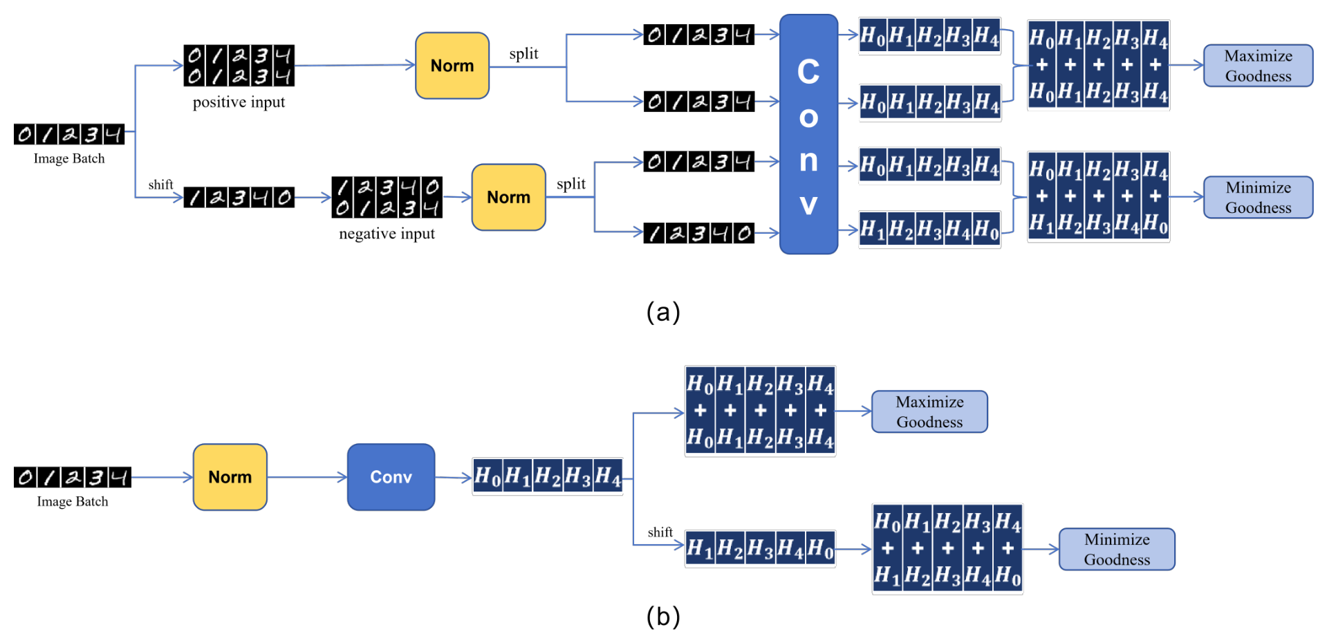
Figure 2.
Illustration of input distribution consistency. (a) In SCFF, normalization is applied to concatenated pairs. Splitting negative pairs leads to Distribution Mismatch. (b) In SCSF, normalization is applied to individual samples first, ensuring Consistent Distribution.
Figure 2.
Illustration of input distribution consistency. (a) In SCFF, normalization is applied to concatenated pairs. Splitting negative pairs leads to Distribution Mismatch. (b) In SCSF, normalization is applied to individual samples first, ensuring Consistent Distribution.
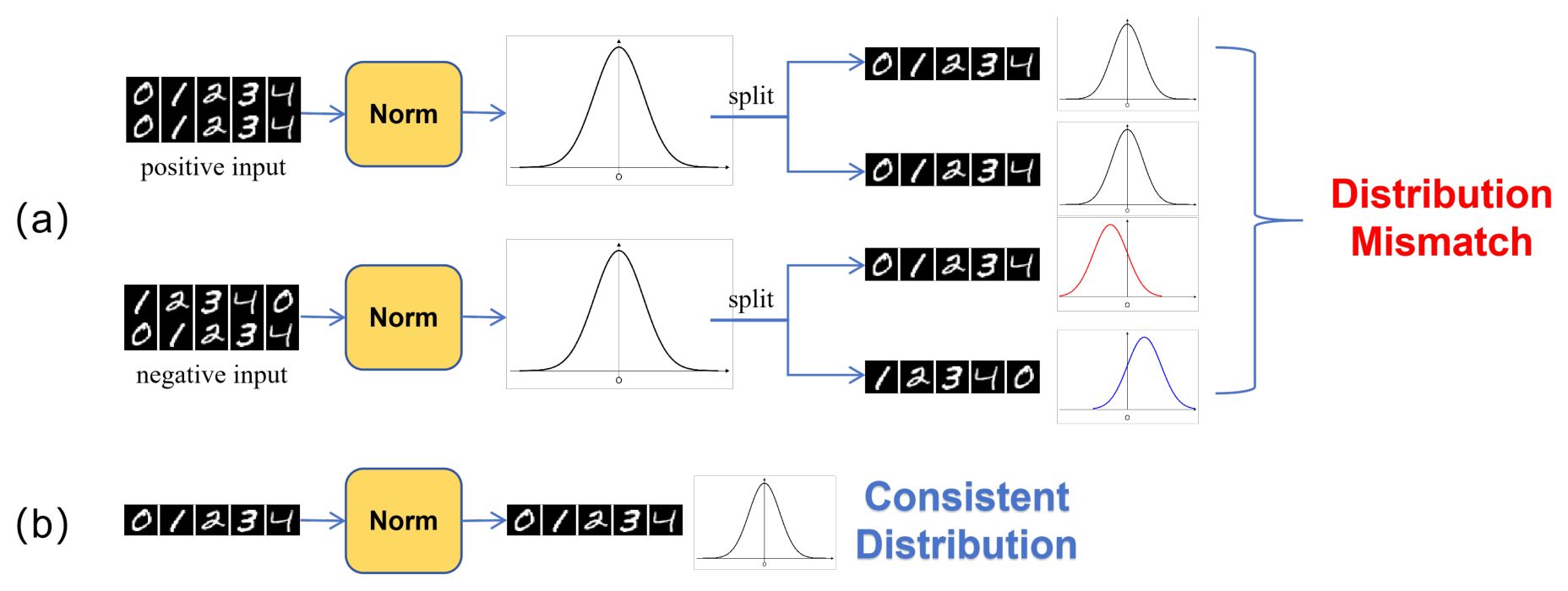
Figure 3.
Training forward-pass computational cost (GFLOPS) across different input resolutions. Benchmarks use a single convolutional layer matching CIFAR-10, STL-10, and Tiny-Imagenet sizes. SCSF reduces cost by 75%.
Figure 3.
Training forward-pass computational cost (GFLOPS) across different input resolutions. Benchmarks use a single convolutional layer matching CIFAR-10, STL-10, and Tiny-Imagenet sizes. SCSF reduces cost by 75%.
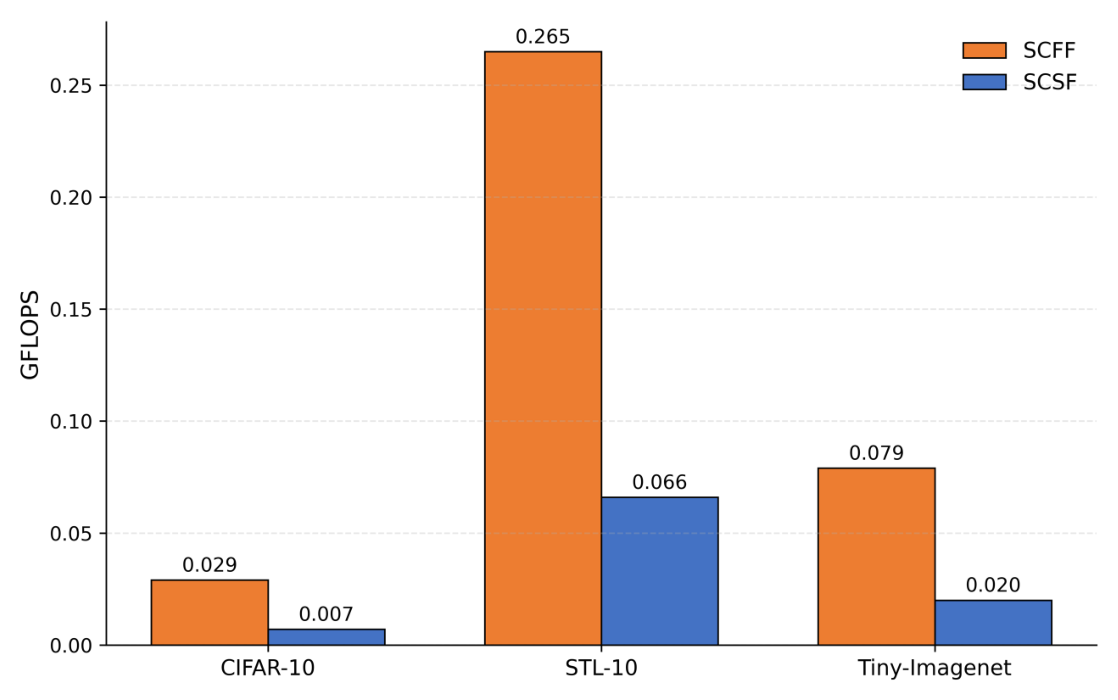
Figure 4.
Training forward-pass throughput (FPS) across different input resolutions. Measured under identical layer-level settings.
Figure 4.
Training forward-pass throughput (FPS) across different input resolutions. Measured under identical layer-level settings.
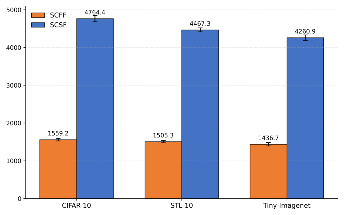
Table 1.
ACCURACY COMPARISON WITH REPRESENTATIVE BACKPROPAGATION-ALTERNATIVE AND LOCAL LEARNING ALGORITHMS (%).
Table 1.
ACCURACY COMPARISON WITH REPRESENTATIVE BACKPROPAGATION-ALTERNATIVE AND LOCAL LEARNING ALGORITHMS (%).
| Algorithm | Unsupervised | CIFAR-10 | STL-10 | Tiny-ImageNet |
|---|---|---|---|---|
| HardHebb (Miconi et al. 2021)[11] | √ | 64.8 | - | - |
| HardHebb (Lagani et al. 2021)[12] | √ | 65.9 | - | - |
| Hebb-CHU[14] | √ | 50.8 | - | - |
| Hebb-PNorm[15] | √ | 72.2 | 76.2 | - |
| SoftHebb[13] | √ | 80.3 | - | - |
| SigProp[28] | × | 91.6 | - | - |
| PEPITA[29] | × | 53.8 | - | - |
| Act.Learning[30] | √ | 58.7 | - | - |
| DFA[20] | × | 73.1 | - | 32.1 |
| DKP[31] | × | - | - | 35.8 |
| EqProp (Laborieux et al. 2021)[17] | × | 88.6 | - | - |
| EqProp (Liu et al. 2024)[18] | √ | 71.5 | - | - |
| DualProp[19] | × | 92.3 | - | - |
| BioSSL[32] | √ | 72.7 | 68.8 | - |
| CLAPP[33] | √ | - | 73.6 | - |
| SCFF[2] | √ | 80.8 | 77.3 | 35.7 |
| SCSF (Ours) | √ | 80.8 | 77.4 | 35.9 |
Disclaimer/Publisher’s Note: The statements, opinions and data contained in all publications are solely those of the individual author(s) and contributor(s) and not of MDPI and/or the editor(s). MDPI and/or the editor(s) disclaim responsibility for any injury to people or property resulting from any ideas, methods, instructions or products referred to in the content. |
© 2026 by the authors. Licensee MDPI, Basel, Switzerland. This article is an open access article distributed under the terms and conditions of the Creative Commons Attribution (CC BY) license (http://creativecommons.org/licenses/by/4.0/).
Copyright: This open access article is published under a Creative Commons CC BY 4.0 license, which permit the free download, distribution, and reuse, provided that the author and preprint are cited in any reuse.


