

Submitted:
05 July 2026
Posted:
06 July 2026
You are already at the latest version
Abstract
Traditional Deep Learning (DL) models for single-image super-resolution (SISR) employ upsampling techniques such as interpolation, transpose convolution, or pixel-shuffle operations.
These upsampling techniques are not explicitly aware of the frequency domain structure, leading to a loss of finer details.
As a result, edges and structural high-information details are often not preserved.
To address this limitation, we propose to introduce an the Inverse Discrete Wavelet Transform (IDWT) based upsampling approach, with a U-Net architecture as a case study.
To this end, the encoder's downsampling part is replaced by the Discrete Wavelet Transform (DWT), and the decoder's upsampling part is replaced by the IDWT for ×2 single-image super-resolution.
In the decoder's upsampling part, we propose a learned channel-splitting mechanism that partitions the feature map into the LH, HL, and HH sub-bands.
The idea is to learn the high frequency sub-bands from the input by assuming the later to be an LL sub-band; the mechanism thus predicts the lost high-frequency wavelet information prior to IDWT reconstruction.
The wavelet-based U-Net we propose utilizes DWT and IDWT to maintain high-frequency details, including edges and textures, thereby improving the quality of single-image super-resolution.
Our model was trained on the DIV2K dataset, and all experiments were conducted under identical and controlled training settings across all baseline variants.
Experimental results on natural-image and text-image benchmark datasets demonstrate that the proposed wavelet-based U-Net model achieves competitive and superior reconstruction performance for x2 super-resolution.
In addition to the quantitative improvements in shape of PSNR and SSIM, visual comparisons further indicate that the proposed method reconstructs sharper and more detailed image structures. These findings suggest that integrating a wavelet transform into encoder-decoder networks helps preserve high-frequency details more effectively, providing an efficient and high-quality solution for single-image super-resolution.
Keywords:
single-image super-resolution (SISR)
; discrete wavelet transform (DWT)
; U-Net
; convolutional neural network (CNN)
; encoder–decoder architecture
; image upscaling
1. Introduction
Artificial Intelligence (AI) is rapidly transforming the world and significantly improving the processing capabilities of computer vision systems. Over the last few years, these technologies have matured enough to deploy in applications spanning a wide range of areas; including vehicle detection [1], real-time object detection/tracking in Unmanned Aerial Vehicles (UAVs) [2], pathological image segmentation, and knowledge distillation [3]. Many of these applications rely on Super-resolution (SR) whereby a high-resolution (HR) image is reconstructed from low-resolution (LR) input(s) [4] to improve image clarity, identify ground targets, and extract fine-grained visual details that are lacking in original LR inputs [5,6]. SR can be broadly categorized into three major types: single-image SR (SISR), video SR, and multi-image SR. Usually, higher-quality reconstruction is required in scenarios where only limited LR data are available. For this reason, SISR has become one of the most studied research topics in computer vision and image processing [7].
In recent years, U-Net [8] has emerged one of the popular SR tool. It was originally conceived for biomedical image segmentation and has an encoder-decoder architecture that employs convolutions. The underlying idea was to use skip connections in order to compensate for the fine spatial information lost during the downsampling phase. Even with limited annotated data, the model achieved enviable performance using data augmentation for biomedical segmentation.
Building upon this foundation, the standard U-Net decoder relies on transpose convolution, pixel-shuffle, and bilinear interpolation for upsampling. However, these operations function entirely in the pixel domain and lack explicit frequency awareness, making it difficult to recover high-frequency details such as edges and textures and other fine details. This may result in information loss during down-sampling and reduce overall reconstruction quality.
To address the above limitation, we propose a frequency-aware wavelet-based method to improve U-Net in which the standard encoder down-sampling and decoder up-sampling operations are replaced with Discrete Wavelet Transform (DWT) and Inverse Discrete Wavelet Transform (IDWT), respectively. Rather than learning to up-sample pixel values directly, the network is trained to predict the missing high-frequency wavelet sub-bands, namely LH, HL, and HH, from the available LR input, assuming it to be the low-frequency LL sub-band. The final reconstruction is performed using a mathematically exact IDWT, a lossless operation rather than a learned approximation, thereby preserving spatial and structural fidelity. This design achieves improved Peak Signal-to-Noise Ratio (PSNR) and The Structural Similarity Index (SSIM) for SR across all tested baselines, including pixel-shuffle, transposed convolution, bilinear and bi-cubic interpolation.
The main contributions of this work are summarized as follows:
- We propose a wavelet-based U-Net framework that integrates DWT and IDWT as frequency-aware replacements for the standard encoder-decoder operations, enabling lossless high-frequency detail preservation for SISR reconstruction.
- We introduce a flexible learned feature split concept that constrains the network to predict missing high-frequency wavelet sub-bands (LH, HL, HH) from the spatial domain feature map; combined with mathematically exact IDWT reconstruction, it reduces the learning burden while achieving superior PSNR and SSIM over all baselines under identical training conditions.
- Extensive experiments on multiple standard SR benchmarks, including Set5, Set14 and BSD100,ICDAR2003. The results also demonstrate that our method competes with state-of-the-art SR techniques while effectively retaining high-frequency details, edges, textures, and structural features.
The rest of the paper is arranged as follows. Section 2 gives a brief overview of the concepts necessary to understand the article. The literature survey is presented in Section 3, while Section 4 presents our methodology in detail. The ensued results and their analyses are presented in Section 5 and Section 6 concludes the paper.
2. Background
The fundamental operation in SISR is the estimation of missing pixel values in an HR grid corresponding to the input LR image. Traditionally, the spatial resolution was realized through a predefined and a weakly constrained mathematical mapping that risks to miss the extremely high frequency information mapped to its HR counterpart. Over the years, SR techniques have evolved from simple mathematical interpolations to very sophisticated DL approaches, thanks to the advent of Generative AI.
2.1. Upsampling in SISR
Upsampling an image during SISR can be broadly classified as interpolation oriented and DL based.
2.1.1. Interpolation Based Upsampling
Here are some of the well-known interpolation methods that are also useful for other geometric transformation tasks such as rotation [9][10]:
- Nearest Neighbor Interpolation copies the nearest pixel values. This simple interpolation approach assigns each unknown HR pixel the value of its nearest LR pixel. For a upscale, each LR pixel is replicated in a block of identical HR pixels. While this method is fast and produces a closed-form solution, the resulting SR images are of low visual quality due to blocky artifacts.
- Bilinear Interpolation computes a weighted average of the four nearest neighbors. This method extends the nearest-neighbor approach by performing a linear interpolation along both horizontal and vertical axes. Each unknown HR pixel value is estimated as a weighted average of it’s 4-neighbors in LR, where the weight is proportional to the inverse distance from each neighbor. This method produces a smoother output than the nearest-neighbor but still lacks the ability to recover sharp edges.
- Bicubic Interpolation uses sixteen neighboring pixels and cubic weighting. The bicubic interpolation considers 16-neighbors instead of four. A smooth cubic polynomial is fitted over this neighborhood to estimate each HR pixel intensity. As a standard SR baseline, bicubic interpolation generally outperforms bilinear interpolation thanks to its larger support and the use of interpolation kernels with negative coefficients, which help preserve image details and produce sharper edges [11]. However, it still relies on a fixed polynomial approximation of unknown pixel values rather than learning image structures and textures from data.
On another note, interpolation-based upsampling [12] operates on fixed handcrafted kernel values with no learning capacity. These methods tend to produce smooth and blurred outputs, lacking the ability to recover fine texture and edge details. While computationally inexpensive, they may not achieve high reconstruction accuracy for SR tasks where the recovery of unknown pixel values is the primary objective.
2.1.2. DL Based Upsampling Methods
-
Transpose convolution is a learnable upsampling technique that increases the spatial resolution of feature maps through trainable filters:where:
- X is the input feature map,
- Y is the upsampled output,
- K is the learnable kernel,
- s is the stride.
Compared to the fixed mathematical methods, it is computationally more expensive because it operates in a multi-dimensional space, performing convolution-based operations to compute new pixel values from existing feature representations. However, this learning capacity allows it to recover spatial details that fixed-rule methods may not. It has a structural problem, however; when the kernel size and stride overlap unevenly, the response may be typically non-uniform if different output pixels are received that are contributing to different numbers of input locations. This produces the checkerboard artifacts; the overlapping learned kernel and overlap patterns become uniformly distributed over the image. -
Pixel-Shuffle (also known as sub-pixel convolution) is a highly efficient technique for spatial upsampling in Convolutional Neural Networks (CNNs), often used in SR to increase the spatial resolution of feature maps. It works by rearranging the depth dimension (channels) of an LR feature map into spatial positions, effectively transforming a feature map into an HR output.PixelShuffle reshapes it intoUnlike methods that rely on explicit interpolation or trainable upsampling, Pixel-Shuffle operates by, 1) increasing the channel dimension using standard convolution to (where s is the upscale factor), and 2) rearranging these channels into spatial pixels.
2.2. Discrete Wavelet Transform (DWT)
When a 2D DWT is applied to an image, it produces four frequency sub-bands at each level [13]; LL (low-frequency), LH (horizontal edges), HL (vertical edges), and HH (diagonal details), as illustrated in Figure 1 for a grayscale image. The 2D IDWT reconstructs the original image from all four [14] sub-bands. Any missing sub-band prevents full recovery [15]. Mathematically, an image of size (say is:
where
After one-level 2D-DWT:
where each sub-band has size:
Let:
- L = low-pass filter
- H = high-pass filter
We get 2D-DWT after applying filters on rows and columns horizontally and vertically.
-
LL sub-bandLow-pass in rows and low-pass in columns:This sub-band contains a low-frequency approximation of the image while the main global structure and smooth content.
-
LH sub-bandLow-pass in rows and high-pass in columns:This band contains information about horizontal edges that is captured because it preserves low-frequency variations in one direction and high-frequency variations in the other.
-
HL sub-bandHigh-pass in rows and low-pass in columns:This sub-band contains only vertical edge information.
-
HH sub-bandHigh-pass in rows and high-pass in columns:This sub-band contains high-frequency diagonal details, such as sharp textures, corners, and fine structures.
Hence, for a image:
or equivalently,
One can also write it as:
with each block being .
From a input, after a one-level 2D-DWT decomposion, the image is partitioned into four sub-bands , , , and of with the component representing the low frequency approximation while the other bands representing the horizontal, vertical and diagonal high frequency details.
2.3. The U-Net
The standard U-Net [8] is a fully convolutional network which owes its name to its unique symmetric U-shaped architecture that predicts a class label for every individual pixel in an input image. As illustrated in Figure 2, it has the following main components:
- Encoder path,
- Bottleneck,
- Decoder path,
- Skip connections,
- Final output layer.
The lower layers of the U-net form an encoder path consisting of a series of down-sampling operations, through conv2D and max-pooling layers, that progressively compress the spatial information into a compact latent features representation via a bottleneck. The upper layers form the decoder path and consists of four blocks, each beginning with a transposed convolution that doubles the spatial dimensions of the feature map, followed by skip connections that concatenate encoder features of the corresponding resolution to preserve spatial detail while up-sampling the features.
The U-Net decoder relies on transpose convolution, pixel-shuffle, and bilinear interpolation operations for up-sampling. However, these operations function entirely in the pixel domain and lack explicit frequency awareness, making it difficult to recover high-frequency details such as edges and textures while up-sampling. During the encoding process, this information is lost as the operations could not identically down-sample the pixel distribution. This loss of information during the down-sampling process can lead to a reduced overall reconstruction quality.
To address this limitation, it would be expedient to improve the U-Net model by effectively replacing its pixel-domain up-sampling operation with a frequency-aware domain in the form of DWT/IDWT. Rather than training the network to directly learn or up-sample pixel values, instead train it to predict the missing high-frequency wavelet sub-band [LH, HL, HH] coefficients from the available low-frequency LR image. The final reconstruction can be readily performed using a mathematically exact IDWT function, which is a lossless operation rather than any learned approximation. It is expected that this design may yield a potentially improved SR over all the tested baselines, including pixel-shuffle, transposed convolution, as well as the bilinear and bicubic interpolations; based on metrics, like PSNR and SSIM.
3. Related Work
Many DL methods have been proposed in the literature [16] to learn a plausible mapping between LR and HR images. Dong et al. [17] pioneered by proposing their SR convolutional neural network (SRCNN), an end-to-end mapping from LR to HR images that outperformed the bicubic interpolation. The work opened a floodgate of efforts [18,19,20,21], including what the authors called the Efficient Sub-Pixel Convolutional Network (ESPCN) [22], that was claimed to have improved the reconstruction speed and quality by performing upsampling through sub-pixel convolutional layers; by moving the upsampling to the final layer via a sub-pixel convolution. Another work [23] combines a lightweight CNN backbone with efficient multi-head attention transformer and pixel-shuffle upsampling. The approach in [24] is to employ sliding window based self-attention, a hierarchical vision transformer, to model multiscale SR. Yet another effort [25] propose what the authors call an adaptive token dictionary with category-based cross-attention to extend receptive fields beyond local windows; a pixel-domain operation with the token-dictionary mechanism risking increased computational complexity. A CNN-based residual attention network [26] tries to retain global context for SR through context-reasoning attention, constrained by its CNN backbone in modeling long-range dependencies.
The literature is replete with efforts based on the use of DWT in SR. The work in [15] proposed combining wavelet transformation with a deep CNN to predict missing high-frequency coefficients in LR images for improved SR reconstruction. Another effort [27] employs a GAN-based SR model that predicts wavelet subband residuals in the frequency domain for better edge and texture recovery, although there is a risk of hallucinating artificial details. To improve the resolution of medical images, especially brain Magnetic Resonance Imaging (MRI), images a SwinV2 [28] transformer based method [29] decomposes the LR input via DWT, extracts deep features using the residual blocks and reconstructs the corresponding HR image through IDWT. The authors in [30] combine spatial-domain learning with wavelet-domain refinement, by employing an Artificial Neural Network (ANN) with bilinear interpolation, for shallow feature extraction, and DWT/IDWT for enhancing the coarse structures. After upsampling the LR input by PixelShuffle, the method in[31] applies DWT to decompose it into frequency sub-bands, which are passed through residual blocks built on the Heat Conduction Operator (HCO) to model long-range spatial dependencies in the deep feature extraction stage. Finally, the refined features are reconstructed back into a high-resolution image using IDWT. The work in [32] uses 2D-DWT to explicitly separate the input into four frequency channels (LL, LH, HL, HH) before the network, reducing training difficulty, then applies lightweight Residual Attention Blocks with channel and spatial attention plus multi-kernel convolutions to adaptively aggregate multi-scale features efficiently.
A DWT/IDWT-based feature reconstruction [33] work utilises a wavelet-enhanced U-Net model for medical image SR and claims to restore fine anatomical details and improve multi-scale feature extraction, edge preservation, and texture recovery. In order to enhance Computed Tomography (CT) images, the work in [34] fuses the LR image with its DWT-extracted high-frequency (HH) component before feeding it to their CNN. Remote sensing images are enhanced in [35] by using DWT to decouple deep features into low-frequency (LF) and high-frequency (HF) components, Their architecture uses self-attention for LF, CNN for HF and cascades multi-level wavelet units to expand the receptive field and capture multi-scale context. A Bayesian Nonparametric (BNP) method [36] estimates DWT filter-bank coefficients for SISR using a Hierarchical Dirichlet Process with blocked Gibbs Sampling in order to exploit inter-scale and intra-scale statistical dependencies of wavelet sub-bands, while simultaneously using a Compound Poisson Process to model and remove Poisson noise within each wavelet scale during reconstruction. Yet another paper[37] proposes a GAN with a DWT-based generator that super-resolves LR label maps into refined HR weak reference maps, enabling weak-supervised learning without requiring detailed ground-truth annotations. For facial SR, the authors in [38] use a U-shaped CNN with depth-separable convolutions and a double branch distillation fusion wherein DWT/IDWT are applied to extract and retain high-frequency facial detail information.
The first efforts in Generative Artificial Intelligence (GenAI) include [39], an edge-enhanced Generative Adversarial Network (GAN) for remote sensing SR, but large upscaling factors create information gaps that complicate training and limit reconstruction under constrained conditions. With the advent of attention/transformer based methods, the SR research has taken a new turn and in this context, a group of related methods from one team [1,40,41] relies on window-based self-attention and overlapping cross-attention within residual groups to capture larger receptive fields for HR reconstruction. Cao et al. [42] enhanced U-Net for super-resolution by integrating wavelet transforms, learning multi-scale wavelet features to simplify low-to-high resolution mapping. Their use of inverse wavelet transforms during upsampling improves sparsity and feature richness, demonstrating the effectiveness of wavelet prediction—aligning with our DWT- and IDWT-based approach for preserving high-frequency details. Another effort [43] builds a lightweight U-Net with DWT based encoder/decoder to achieve real-time SR on resource-constrained drone hardware. For the sake of efficiency, without affecting the structural edges. In [44], the authors introduced a modified U-Net for single-image super-resolution, eliminating batch normalization and reducing the depth of convolutional layers in each block to decrease computational overhead. To mitigate the blurred edges often produced by by networks optimized with mean squared error (MSE), they incorporated a mixed gradient loss that combines MSE with a weighted mean gradient error term. Although this approach enhanced edge sharpness, the architecture remains confined to the spatial domain, lacking an explicit mechanism to separate or prioritize high-frequency content. This limitation restricts its capacity to recover fine structural details when compared to frequency-aware methods. The GAN-based method in [45], replaces the standard discriminator with a U-Net-based discriminator and spectral normalization to fuse multi-scale real/fake image features. A transformer based effort [46] employs a combination of sparse attention (for global features) and local dense attention (for local features), integrated into a U-Net with multi-resolution paths (for multi-scale features). Another method [47] introduces shuffle pooling to improve down-sampling and feature extraction by combining it with the U-Net’s encoder–decoder structure. Another transformer based method in [48] applies adaptive token sparsification and early-exit halting to reduce compute while operating entirely in the pixel domain without frequency-domain awareness. A diffusion based work [49] combines a diffusion model with implicit neural representation for continuous-scale SR via coordinate-based upsampling, at the cost of higher compute and slower inference. A comparison based summary of the methods is illustrated in Table 1.
4. Methodology
The standard U-Net architecture, designed for super-resolution, employs an encoder that progressively reduces spatial resolution through max pooling, average pooling, and stridden convolution, while compressing the spatial dimensions. These operations are inherently lossy, with max pooling retaining only the most prominent activations, whereas stridden convolution discarding some spatial information. As a consequence, high-frequency spatial information – such as edges, fine textures, and diagonal structures – is affected, as the feature maps propagate towards the bottleneck. We build upon the lightweight modified U-Net from Lu and Chen [44] as our backbone, preserving its reduced-parameter encoder-decoder structure. Our extension introduces DWT decomposition in the encoder and a learned channel-split mechanism in decoder that adaptively weights each frequency sub-band before IDWT reconstruction. Unlike the original, which relies on a mixed gradient loss for edge sharpness, our architecture explicitly models frequency content, enabling the network to prioritize high-frequency sub-bands where structural detail loss is most significant.
The proposed network, as illustrated in Figure 3, operates in the wavelet domain rather than in the pixel domain. Given an LR input of size , the model does not directly predict a pixel output. Instead, it learns the missing high-frequency wavelet sub-bands [LH, HL, and HH] while preserving the available low-frequency LL sub-band. The IDWT is then applied to all four sub-bands to reconstruct a full HR image. This formulation enables the network to learn frequency-domain information more effectively, since the reconstruction target is structured and mathematically interpretable rather than a direct pixel prediction problem. By substituting the standard encoder-decoder operations in U-Net with DWT and IDWT, respectively, we are vying to empirically demonstrate that this approach outperforms conventional upsampling methods under identical training conditions. Furthermore, constraining the network to treat the input as an LR through the proposed architectural optimization reduces the learning burden while maintaining superior reconstruction quality across all tested configuration variants.
Step 1: Network Input and Initial Feature Extraction
The proposed network performs super-resolution in the wavelet domain. For each training sample, two versions of the low-frequency wavelet component are used: the normalized LR component and the raw LR component . Both have the same spatial and channel dimensions:
The normalized component is used as the network input because it provides a stable scale for learning, while is preserved for the final inverse wavelet reconstruction. The input first passes through an initial double-convolution block, which maps the 3-channel LR input to 64 shallow feature channels:
This stem block extracts low-level spatial and structural features from the normalized LR input. The output is also retained as a skip connection for the decoder stage.
Step 2: Wavelet-Based Encoder (DWT ↓)
The encoder progressively reduces the spatial resolution while increasing the number of feature channels. In conventional U-Net, this reduction is commonly performed using max-pooling or strided convolution. In the proposed architecture, the downsampling operation is replaced by a DWT-based block (Figure 4. For an input feature map , the DWT decomposes the feature map into four sub-bands:
The four sub-bands are concatenated along the channel dimension, increasing the channel count from C to :
The concatenated representation is then passed through a double-convolution block. This block applies two consecutive convolution layers, each followed by LeakyReLU activation. It refines the concatenated wavelet features, changes the channel depth from the input channel size to the required output channel size, and produces the downsampled feature map:
where denotes the LeakyReLU activation, * denotes a convolution operation, and ∥ denotes channel-wise concatenation. This design explicitly represents both low-frequency and high-frequency components before spatial reduction. Therefore, edge-, texture-, and structure-related responses are carried through the , , and sub-bands instead of being directly suppressed by pooling. In the implemented encoder, two DWT-based downsampling stages are used. The first stage receives the output of stem and reduces the spatial size from to , while increasing the channel depth from 64 to 128:
The second stage further reduces the feature resolution from to and increases the channel depth from 128 to 256:
Thus, the encoder transforms the initial feature representation as:
Step 3: Extended Bottleneck with Channel Attention (Residual Channel Attention Block (RCAB) Stack)
After the encoder, the feature map reaches the lowest spatial resolution of the network, . This central part of the encoder–decoder architecture is used as the bottleneck because it operates on the most spatially compact representation before the decoder begins reconstruction. At this stage, the feature map has already been compressed spatially; therefore, the bottleneck first applies a double-convolution block to increase the feature depth from 256 channels to 512 channels. This increases the representational capacity of the model while keeping the computational cost manageable due to the reduced spatial size. The bottleneck transformation is expressed as:
The purpose of this channel expansion is to learn a deeper and richer feature representation before decoding. Since the model later predicts the missing high-frequency wavelet sub-bands, the expanded bottleneck representation (Figure 5) helps encode structural, edge-related, and frequency-relevant information at the most compact spatial scale.
The bottleneck feature map is then refined using a stack of RCABs. In the implemented configuration, the stack contains 30 RCABs. It is important to note that the channel expansion from 256 to 512 occurs only in the bottleneck double-convolution block. The RCAB stack does not further expand the number of channels; instead, it refines and reweights the existing 512-channel feature representation.
Each RCAB contains a residual convolutional branch followed by a channel attention module. The residual branch can be written as:
where denotes two convolutional layers used for residual feature extraction. The channel attention (CA) module is then applied to the residual feature r, and the RCAB output is obtained through residual addition:
For a feature tensor , the CA module first applies global average pooling (GAP):
This operation compresses only the spatial dimensions into , while preserving the number of channels C. The pooled descriptor is then passed through a lightweight channel-wise Multilayer Perceptron (MLP) followed by a sigmoid activation to obtain one attention weight for each channel:
The attention weights are multiplied with the residual feature map through channel-wise multiplication:
where denotes the sigmoid activation and ⊙ denotes channel-wise multiplication with broadcasting over the spatial dimensions. Thus, channel attention does not increase or decrease the number of channels. It only learns channel-wise importance weights and rescales the existing feature channels.
In the bottleneck of the proposed architecture, this means that the RCAB stack receives and outputs feature maps with the same channel depth:
Therefore, the bottleneck first increases the channel depth through the double-convolution block and then uses the RCAB stack to refine the 512-channel representation. This allows the model to emphasize informative feature channels before decoding, which is useful for wavelet-domain super-resolution because different channels may contribute differently to the later prediction of , , and high-frequency sub-bands.
Step 4: Wavelet-Based Decoder (IDWT ↑)
The decoder restores the spatial resolution in a reverse multi-scale manner. Instead of using transposed convolution or pixel-shuffle, the proposed decoder uses IDWT-based upsampling blocks, as illustrated in Figure 6. At each decoder stage, the input feature channels are divided into four equal groups and treated as pseudo wavelet sub-bands. For an input tensor with C channels, let . The four channel groups are given by:
These four groups are passed through IDWT to double the spatial resolution:
The upsampled feature map is then concatenated with the corresponding encoder skip connection and refined using a double-convolution block:
The first decoder stage receives the bottleneck output with 512 channels at . After IDWT upsampling, the feature map is restored to , concatenated with the encoder skip feature , and fused to produce 256 output channels:
The second decoder stage restores the resolution from to . It uses the skip connection from the stem level and produces 128 output channels:
Thus, the decoder transforms the bottleneck feature representation as:
This decoder design provides a wavelet-consistent upsampling mechanism. The skip connections help recover spatial information from earlier encoder stages, while the IDWT-based blocks restore the feature resolution in a structured sub-band form.
Step 5: High-Frequency Sub-Band Prediction Head
After the two IDWT-based decoder stages, the feature map returns to the LR spatial resolution of . A refinement block is then applied before predicting the final wavelet high-frequency sub-bands. As shown in Figure 7, this refinement block contains two additional RCABs, followed by a convolution and LeakyReLU activation. It reduces the decoder feature depth from 128 channels to 64 channels:
The refined feature map is then passed to a final convolutional prediction head. This head outputs 9 channels, corresponding to three red-green-blue (RGB) channels for each of the three high-frequency wavelet sub-bands:
Here, is a learnable scalar initialized to . This scaling factor reduces the magnitude of the initial high-frequency predictions and may improve early training stability.
The 9-channel output is then divided into three groups using channel-wise chunking:
Therefore, the network does not directly predict the final high-resolution RGB image. Instead, it predicts the missing wavelet detail components , , and , which are later combined with the preserved raw LR component.
Step 6: Final HR Reconstruction via IDWT
The final super-resolved image is reconstructed using IDWT. In this step, as illustrated in Figure 8, the original raw LR is combined with the predicted high-frequency sub-bands:
The input sub-bands to the final IDWT all have the same spatial size and channel count:
After IDWT reconstruction, the output becomes:
This final reconstruction step is important because is not predicted by the network; it is directly reused in its original coefficient scale. Thus, the low-frequency structure is preserved through the raw LR component, while the network focuses its output prediction on the missing high-frequency detail sub-bands. The complete model can therefore be expressed compactly as:
Here, denotes the proposed wavelet U-Net. The normalized LR component is used for learning the high-frequency sub-band prediction, whereas the raw LR component is used only during the final IDWT reconstruction. Consequently, the model performs super-resolution by reconstructing a RGB image from a LR representation and the predicted high-frequency wavelet details. Table 2 sums up our modified U-Net pipeline.
5. Experimental Setup and Results
For the sake of our experiments, we have used images from standard datasets. However, each HR RGB image was first resized to to serve as the ground truth (GT) and a single-level 2D-DWT was then applied channel-wise to each such image to get our LR inputs that upon processing by our network, gave us the HR output. Synthetic blur or noise degradation was not added during this process.
5.1. Training and Benchmark Datasets
The proposed model was trained and validated using the DIV2K [55] dataset. DIV2K contains 800 high-resolution training images and 100 validation images. Each PNG image was center-cropped into a square shape to handle different aspect ratios, and then resized to using bicubic interpolation. The resized images were saved as float32 tensors in the range . The standard DIV2K split was used, with 800 images for training and 100 images for validation, without any test set augmentation. In this work, the high-resolution image size is , while the low-resolution input is represented by the LR image of size , corresponding to a scaling factor of .
In SISR related works, standard benchmark datasets are very important for a fair comparison with state of the art methods. Commonly used benchmark datasets include Set5, Set14, and BSD100. These datasets are among the most widely used datasets in the super-resolution literature and have been used for evaluating DL-based models such as SRCNN [17] and later methods.
Set5 [56] is a small benchmark dataset containing 5 classic images, including baby, bird, butterfly, head, and woman. Although it is small in size, it contains rich structural information, edges, and complex image details. Therefore, PSNR and SSIM evaluation on Set5 is commonly reported in super-resolution research.
Set14 [57] It contains images with different types of visual diversity, including faces, animals, comic art, text, and fine patterns. Due to this variation, Set14 is also a well-known benchmark dataset widely used in super-resolution literature.
BSD100 [58] is a subset of 100 test images from the Berkeley Segmentation Dataset, introduced by Martin et al. in 2001. It is considered a challenging benchmark because it contains natural photographs with diverse textures, irregular edges, and cluttered backgrounds. For this reason, BSD100 is also widely used for evaluating SISR methods.
5.2. Preprocessing
Since no separate ground-truth HR images were available, the original dataset images were used as the HR reference images and were treated as ground truth for training and evaluation. In this work, each original dataset image with spatial resolution was considered as the HR target. The corresponding LR image was generated from the same HR reference image using DWT. Therefore, the LR–HR image pairs were constructed from the dataset itself, where the original image served as the ground-truth HR image and the DWT approximation component served as the LR input.
This process produced the LR approximation image, which was used as the LR input to the proposed network. No synthetic blur or noise degradation was added during this process. The scaling factor was , where the spatial resolution was reduced from to through DWT faimly biorthogonal bior4.4. After training, the network output was used to reconstruct the final SR image at resolution through IDWT.
For normalization, the per-channel mean and standard deviation were computed over the entire training split of LR images. During training and inference, the LR input was standardized as
where and denote the training-split mean and standard deviation, respectively. The raw LR images , without normalization, were separately preserved and directly used in the final IDWT reconstruction.
The training target was the original HR RGB image with shape in the range . The high-frequency subband targets, including LH, HL, and HH, were extracted on-the-fly during training from the HR reference image using the same bior4.4 wavelet and periodization DWT setting. After reconstruction, the generated SR image with resolution was compared with its corresponding original HR reference image for quantitative evaluation using PSNR and SSIM.
5.3. Training Details
The proposed Wavelet U-Net was trained on the DIV2K dataset using paired LR-HR samples. As we do not have separate ground-truth HR original dataset or LR images we did preprocessing. The original dataset image with spatial resolution , and the corresponding LR images of size were used as input to the network. The LR inputs were normalized using training-set statistics, while the raw LR images were preserved separately for final IDWT reconstruction. The model was trained using the Adam optimizer with a learning rate of , batch size of 8, and 100 epochs. The loss function was defined on the reconstructed HR image and predicted high-frequency subbands. The performance was evaluated using PSNR and SSIM on the validation set.
Figure 9 illustrates the training convergence analysis of the proposed DWT/IDWT U-Net model on the DIV2K dataset. The L1 loss, Figure 9(a), decreases steadily, confirming stable learning and reduced pixel-level error. Simultaneously, as can be seen in Figure 9(b,c), the PSNR and SSIM consistently increase, demonstrating that predicting high-frequency wavelet sub-bands prior to IDWT reconstruction effectively minimizes distortion and accurately preserves structural details, like edges, textures, and local image patterns.
Figure 10 compares U-Net decoder variants across four benchmark datasets; viz. Set5, Set15, BSD100, and DIV2K (HRO). The proposed DWT/IDWT-based U-Net achieves the highest PSNR (37.85 dB) (a) and SSIM (0.9596) (b) scores. These results demonstrate that the wavelet-based decoder minimizes distortion and preserves structural details more effectively than conventional upsampling designs.
The Loss function:
where and .
Table 3 presents the main training hyperparameters used for model optimization. The network was trained on the DIV2K dataset using normalized low-resolution inputs of size and corresponding high-resolution targets of size . The Adam optimizer with an initial learning rate of and a batch size of 8 was employed for 100 epochs. Model performance was evaluated using the PSNR and SSIM metrics to assess reconstruction fidelity and structural similarity.
Table 4 summarizes the training and implementation settings used in this study. The proposed model was implemented in PyTorch with PyTorch Lightning and trained on a single Google Colab L4 GPU using mixed-precision computation for improved efficiency. Training was performed for up to 100 epochs using a MultiStepLR scheduler, with the learning rate reduced at epochs 60, 80, and 95. The network employed 30 RCAB blocks and was optimized using a combination of image reconstruction L1 loss and high-frequency subband supervision. To enhance training stability, gradient clipping and exponential moving average (EMA) of model weights were applied. Model performance was evaluated using PSNR and SSIM, while checkpoint selection was based on the highest validation PSNR-Y scores.
PSNR and SSIM are computed on the luma (Y) channel only, following the standard SR evaluation protocol. The Y channel is derived using the standard formula:
A 2-pixel border is shaved from all images before the metric computation to exclude boundary artifacts, consistent with standard SR benchmarks. At validation, EMA generator weights are used instead of the raw training weights, producing more stable metric estimates. Both PSNR and SSIM are reported as epoch-level mean ± standard deviation (std) over the full validation split.
5.4. Comparison with Various Upsampling Approaches in U-Net
Figure 11, Figure 12, and Figure 13 visually compare the proposed method against bicubic interpolation, transposed Convolution, and the baseline U-Net. Magnified regions highlight the differences in fine details. For the lemon image (Figure 11), the proposed model reconstructs sharper edges and textures closest to the ground truth. In the flower image (Figure 11), it recovers detailed petal structures where competing methods cause blurring. Finally, for the human figures (Figure 11), the model accurately preserves object boundaries with fewer artifacts, confirming its superior high-frequency reconstruction capabilities. Overall, the qualitative results demonstrate that the proposed wavelet-based DWT/IDWT U-Net consistently generates visually sharper images with improved detail preservation across diverse scene contents, producing reconstructions that more closely resemble the ground-truth images.
The results presented in Table 5 highlight several important observations. The proposed DWT/IDWT method achieves a PSNR of 30.59 dB, outperforming all baseline approaches. The closest competing method, U-Net combined with bicubic upsampling, attains 29.05 dB, resulting in a performance gain of dB for the proposed approach.
Furthermore, the HR0 baseline of the proposed method, which corresponds to IDWT reconstruction using zero high-frequency sub-bands, already achieves a PSNR of 29.20 dB. This value surpasses the HR0 results of all other methods, including bicubic interpolation, which only reaches 18.08 dB. This observation indicates that the LR-anchored reconstruction provides a significantly stronger initialization even before any learning is applied.
In contrast, transposed convolution yields the lowest performance among the learned methods, with a PSNR of 27.48 dB. This result aligns with prior findings, as transposed convolution is often associated with checkerboard artifacts that degrade reconstruction quality.
For Table 6 (benchmark datasets): The results across the benchmark datasets reveal consistent improvements of the proposed method. The largest PSNR gain is observed on Set5, with an improvement of dB. This dataset contains relatively simple and clean images, where accurate recovery of high-frequency details has a more pronounced impact on performance.
Urban100 exhibits the highest improvement in SSIM, with a gain of , suggesting that the wavelet-based approach is particularly effective at preserving structural information and edge details in urban scenes characterized by repetitive and fine patterns.
In contrast, BSD100 shows the smallest PSNR improvement of dB. This is expected, as natural images with complex textures are inherently more challenging for SR tasks.
5.5. Comparison with State-of-the-Art
To assess the performance of our proposed super-resolution approach, we benchmark its quantitative results against multiple deep learning-based super-resolution techniques, such as SRCNN, FSRCNN, VDSR, DRCN, SRGAN, ESPCN, EDSR, DBPN, UnetSR, and UnetSR+. We also include bicubic interpolation as a baseline for comparison. The evaluation focuses on the upscaling factor, considering PSNR and SSIM as key metrics. The quantitative results for the Set14, BSD300, and ICDAR2003 datasets are summarized in Table 7, where the best-performing results are marked in bold and the second-best are underlined.
Our method achieves the highest PSNR and SSIM scores on Set14, with values of 32.80 dB and 0.9295, respectively. This demonstrates its effectiveness in reconstructing image details and maintaining structural fidelity for natural image benchmarks. On the BSD300 dataset, our approach also delivers the best performance, with 32.30 dB PSNR and 0.9145 SSIM, surpassing all competing methods. Given the diversity of natural scenes, textures, and structural variations in BSD300, these results highlight the robustness of our wavelet-based reconstruction strategy in handling complex image content.
For text-image super-resolution, our method records the highest PSNR on ICDAR2003 at 37.74 dB, along with a competitive SSIM of 0.96. While UnetSR+ achieves a marginally higher SSIM on this dataset, our approach maintains the best PSNR and strong structural similarity. This is particularly significant for text-image super-resolution, where sharp edges, stroke boundaries, and fine character structures are critical for visual clarity. The strong PSNR performance on ICDAR2003 confirms that our method effectively minimizes reconstruction errors while preserving perceptual quality.
Overall, the results confirm that our wavelet-based U-Net delivers strong reconstruction quality across both natural and text-image super-resolution benchmarks. The consistent improvements on Set14 and BSD300, combined with the highest PSNR on ICDAR2003, demonstrate that integrating DWT and IDWT into the reconstruction process enhances the preservation of high-frequency details, such as edges, textures, and fine structures, during encoder-decoder processing. Thus, our method presents an effective solution for single-image super-resolution.
6. Conclusions
This paper presented a wavelet-based U-Net that works for SISR in which conventional encoder-decoder sampling operators were replaced with DWT and IDWT. Under controlled comparisons with standard U-Net variants using bicubic interpolation, transposed convolution, Pixel-Shuffle, and conventional U-Net, the proposed design achieved superior PSNR and SSIM performance. The results indicate that frequency-aware, multi-resolution upsampling improves reconstruction fidelity in a modified encoder–decoder U-Net network. The proposed DWT/IDWT method achieves 37.85 dB PSNR on the Set5 dataset, outperforming all baselines. The closest competitor is U-Net + Bicubic at 35.09 dB, representing a margin of +2.76 dB in favor of the proposed method. The HR0 base line of the proposed method (IDWT) reconstruction with zero high-frequency sub-bands already scores 29.20 dB, which exceeds all other methods’ HR0 results (18.08 dB bicubic). This confirms that the single-image reconstruction provides a substantially stronger starting point prior to any learning. We also introduced the flexible learned feature split concept that constrains the network to predict missing high-frequency wavelet sub-bands (LH, HL, HH) from the high frequency domain feature map.
There are some limitations that could be resolved in the future to improve U-Net SR with DWT/IDWT-based encoder-decoder reconstruction efficiency and usefulness. The evaluation focuses exclusively on one architecture family (U-Net), and further tests across diverse backbone architectures, datasets, and scale factors are needed to establish broader generalizability. We used a fixed family of wavelets, like all experiments we did with the use of bior4.4 mode periodisation. Our method only works on the scale; we have not tested it on multiscale yet. Extending to , , where multi-level wavelet decomposition is still an open direction for future work.
References
- Chen, C.; Wang, C.; Liu, B.e.a. Edge Intelligence Empowered Vehicle Detection and Image Segmentation for Autonomous Vehicles. IEEE Trans. Intell. Transp. Syst. 2023. [Google Scholar] [CrossRef]
- Ding, S.; Wang, H.; Lu, H.; et al. Two Path Gland Segmentation Algorithm of Colon Pathological Image Based on Local Semantic Guidance. IEEE J. Biomed. Health Inform. 2022, 27, 1701–1708. [Google Scholar] [CrossRef]
- Gou, J.; Sun, L.; Yu, B.; et al. Multilevel Attention-Based Sample Correlations for Knowledge Distillation. IEEE Trans. Ind. Inform. 2022, 19, 7099–7109. [Google Scholar] [CrossRef]
- Dong, C.; Loy, C.C.; He, K.; Tang, X. Image Super-Resolution Using Deep Convolutional Networks. IEEE Trans. Pattern Anal. Mach. Intell. 2015, 38, 295–307. [Google Scholar] [CrossRef]
- Bilgazyev, E.; Efraty, B.; Shah, S.K.; Kakadiaris, I.A. Improved Face Recognition Using Super-Resolution. In Proceedings of the 2011 International Joint Conference on Biometrics (IJCB), Piscataway, 2011; pp. 1–7. [Google Scholar]
- Mehdi, S.M.S.; Bernhard, S.; Michael, H. EnhanceNet: Single Image Super-Resolution Through Automated Texture Synthesis. In Proceedings of the International Conference on Computer Vision, Piscataway, 2017; pp. 4491–4500. [Google Scholar]
- Shi, W.Z.; Caballero, J.; Ledig, C.; et al. Cardiac Image Super-Resolution with Global Correspondence Using Multi-Atlas PatchMatch. Proc. Med. Image Comput. Comput.-Assist. Interv. (MICCAI) 2013, Vol. 8151, 9–16. [Google Scholar] [CrossRef]
- Ronneberger, O.; Fischer, P.; Brox, T. U-Net: Convolutional Networks for Biomedical Image Segmentation. Proc. Med. Image Comput. Comput.-Assist. Interv. 2015, Vol. 9351, 234–241. [Google Scholar] [CrossRef]
- Lehmann, T.M.; Gonner, C.; Spitzer, K. Survey: Interpolation methods in medical image processing. IEEE Trans. Med. Imaging 2002, 18, 1049–1075. [Google Scholar]
- Magnier, B.; Moradi, B.; Carré, P. Evaluation of Half Gaussian Filter Rotation for Edge Detection. In Proceedings of the 2019 8th European Workshop on Visual Information Processing (EUVIP); IEEE, 2019; pp. 52–57. [Google Scholar]
- Keys, R. Cubic convolution interpolation for digital image processing. IEEE Trans. Acoust. Speech Signal Process. 1981, 29, 1153–1160. [Google Scholar] [CrossRef]
- Getreuer, P. Image Interpolation with Contour Stencils. Image Process. Line 2011, 1, 70–82. [Google Scholar] [CrossRef]
- Mallat, S.G. The wavelet transform, time-frequency localization and signal analysis. IEEE Trans. Pattern Anal. Mach. Intell. 1989, 11, 674–693. [Google Scholar] [CrossRef]
- Taubman, D.; Marcellin, M. JPEG2000: Image compression fundamentals, standards and practice; Springer, 2002. [Google Scholar]
- Guo, T.; Mousavi, H.S.; Vu, T.H.; Monga, V. Deep Wavelet Prediction for Image Super-Resolution. In Proceedings of the IEEE Conference on Computer Vision and Pattern Recognition Workshops (CVPR Workshops), Piscataway, 2017; pp. 104–113. [Google Scholar]
- Hayat, K. Multimedia super-resolution via deep learning: A survey. Digit. Signal Process. 2018, 81, 198–217. [Google Scholar] [CrossRef]
- Dong, C.; Loy, C.C.; He, K.M.; Tang, X.O. Learning a Deep Convolutional Network for Image Super-Resolution. In Proceedings of the European Conference on Computer Vision (ECCV), Berlin, 2014; Vol. 8692, pp. 184–199. [Google Scholar]
- Kim, J.; Lee, J.K.; Lee, K.M. Deeply-Recursive Convolutional Network for Image Super-Resolution. In Proceedings of the Proceedings of the IEEE Conference on Computer Vision and Pattern Recognition (CVPR), 2016; pp. 1637–1645. [Google Scholar]
- Lim, B.; Son, S.; Kim, H.; Nah, S.; Lee, K.M. Enhanced Deep Residual Networks for Single Image Super-Resolution. In Proceedings of the Proceedings of the IEEE Conference on Computer Vision and Pattern Recognition Workshops (CVPRW), 2017; pp. 136–144. [Google Scholar]
- Lai, W.S.; Huang, J.B.; Ahuja, N.; Yang, M.H. Deep Laplacian Pyramid Networks for Fast and Accurate Super-Resolution. In Proceedings of the IEEE Conference on Computer Vision and Pattern Recognition (CVPR), Piscataway, 2017; pp. 624–632. [Google Scholar]
- Zhang, Y.L.; Li, K.P.; Li, K.; et al. Image Super-Resolution Using Very Deep Residual Channel Attention Networks. In Proceedings of the European Conference on Computer Vision (ECCV), Berlin, 2018; pp. 286–301. [Google Scholar]
- Shi, W.; Caballero, J.; Huszar, F.; Totz, J.; Aitken, A.P.; Bishop, R.; Rueckert, D.; Wang, Z. Real-Time Single Image and Video Super-Resolution Using an Efficient Sub-Pixel Convolutional Neural Network. In Proceedings of the Proceedings of the IEEE Conference on Computer Vision and Pattern Recognition (CVPR), 2016; pp. 1874–1883. [Google Scholar]
- Lu, Z.; Li, J.; Liu, H.; Huang, C.; Zhang, L.; Zeng, T. Transformer for Single Image Super-Resolution. In Proceedings of the Proceedings of the IEEE/CVF Conference on Computer Vision and Pattern Recognition Workshops (CVPRW), 2022. [Google Scholar]
- Liu, Z.; Lin, Y.; Cao, Y.; Hu, H.; Wei, Y.; Zhang, Z.; Lin, S.; Guo, B. Swin Transformer: Hierarchical Vision Transformer Using Shifted Windows. In Proceedings of the Proceedings of the IEEE/CVF International Conference on Computer Vision (ICCV), 2021. [Google Scholar]
- Zhang, L.; Li, Y.; Zhou, X.; Zhao, X.; Gu, S. Transcending the Limit of Local Window: Advanced Super-Resolution Transformer with Adaptive Token Dictionary. In Proceedings of the Proceedings of the IEEE/CVF Conference on Computer Vision and Pattern Recognition (CVPR), 2024; pp. 2856–2865. [Google Scholar]
- Zhang, Y.; Wei, D.; Qin, C.; Wang, H.; Pfister, H.; Fu, Y. Context Reasoning Attention Network for Image Super-Resolution. In Proceedings of the Proceedings of the IEEE/CVF International Conference on Computer Vision (ICCV), 2021; pp. 4278–4287. [Google Scholar]
- Mofrad, M.M.; Fatehi, M.H.; Taghizadeh, M.; Jamali, J. Single image super-resolution based on deep networks and wavelet transform. Multimed. Tools Appl. 2025, 84, 30563–30581. [Google Scholar] [CrossRef]
- Liu, Z.; Hu, H.; Lin, Y.; Yao, Z.; Xie, Z.; Wei, Y.; Ning, J.; Cao, Y.; Zhang, Z.; Dong, L.; et al. Swin Transformer V2: Scaling Up Capacity and Resolution. arXiv 2022, arXiv:cs. [Google Scholar]
- Cestola, P.; Othmani, A.; Lagzouli, A.; Sansalone, V.; Teresi, L. DWTSRNet: Discrete Wavelet Transform Super Resolution Network for Medical Single Image Super-Resolution. Proc. 2024 IEEE Int. Conf. Bioinform. Biomed. (BIBM) 2024, 4861–4868. [Google Scholar] [CrossRef]
- Karayaka, M.; Muhammad, U.; Laaksonen, J.; Hoque, M.Z.; Seppanen, T. A Dual-Domain Convolutional Network for Hyperspectral Single-Image Super-Resolution. arXiv 2025, arXiv:2512.09546. [Google Scholar]
- Zhang, J.; Gao, L.; Xiao, Z. vHeatSR: Vision Model Based on Heat Conduction for Medical Image Super-Resolution. In Proceedings of the 2025 IEEE International Conference on Bioinformatics and Biomedicine (BIBM), 2025. [Google Scholar]
- Xue, S.; Qiu, W.; Liu, F.; Jin, X. Wavelet-based residual attention network for image super-resolution. Neurocomputing 2020, 382, 116–126. [Google Scholar] [CrossRef]
- Tian, W.; Zhang, X. A Study on Medical Image Super-Resolution with Wavelet Transform and U-Net. In Proceedings of the 2025 7th International Conference on Control and Computer Vision. IEEE, 2025. [Google Scholar] [CrossRef]
- Wang, Q.S.; Ma, Q. Super-resolution reconstruction algorithm for medical images by fusion of wavelet transform and multi-scale adaptive feature selection. IET Image Processing, 2024. [Google Scholar]
- Yu, J.; Dou, Y. Wavelet-based Frequency Decoupling Refinement Network for Remote Sensing Image Super Resolution. In Proceedings of the Proceedings of the 2025 7th International Conference on Control and Computer Vision. ACM, 2025. [Google Scholar] [CrossRef]
- Sadaghiani, A.V.K.; Sargolzaei, H.; Forouzandeh, B. Novel Computation-Efficient Single-Image Super-Resolution Based on Hierarchical Dirichlet Process Using Compound Poisson Process. Int. J. Image Graph. 2026, 26, 2650027. [Google Scholar] [CrossRef]
- Singh, A.; Bruzzone, L. Wavelet-Based Deep Generative Framework for Super Resolution of Low-Resolution Labelled Maps and Weak-Supervised Learning. IEEE Trans. Geosci. Remote Sens. 2025. [Google Scholar] [CrossRef]
- Wang, T.; Xiao, Y.; Cai, Y.; Gao, G.; Jin, X.; Wang, L.; Lai, H. UFSRNet: U-shaped face super-resolution reconstruction network based on wavelet transform. Multimed. Tools Appl. 2024, 83, 67231–67249. [Google Scholar] [CrossRef]
- Jiang, K.; Wang, Z.; Yi, P.; et al. Edge-Enhanced GAN for Remote Sensing Image Super-Resolution. IEEE Trans. Geosci. Remote Sens. 2019, 57, 5799–5812. [Google Scholar] [CrossRef]
- Chen, X.; Wang, X.; Zhou, J.; Qiao, Y.; Dong, C. Activating More Pixels in Image Super-Resolution Transformer. In Proceedings of the Proceedings of the IEEE/CVF Conference on Computer Vision and Pattern Recognition (CVPR), 2023. [Google Scholar]
- Chen, Z.; Zhang, Y.; Gu, J.; Kong, L.; Yang, X.; Yu, F. Dual Aggregation Transformer for Image Super-Resolution. In Proceedings of the Proceedings of the IEEE/CVF International Conference on Computer Vision (ICCV), 2023; pp. 12278–12287. [Google Scholar]
- Cao, J.; Chen, Z.; Cui, H.; Ji, X.; Wang, X.; Liang, Y.; Tian, Y. Improved wavelet prediction superresolution reconstruction based on U-Net. IET Image Process. 2023, 17, 3464–3476. [Google Scholar] [CrossRef]
- Chen, C.L.; Yao, H.L.; Jian, B.L. Discrete Wavelet Transform Sampling for Image Super Resolution. J. Inf. Telecommun. doi to be confirmed. 2024. [Google Scholar] [CrossRef]
- Lu, Z.; Chen, Y. Single Image Super-Resolution Based on a Modified U-Net with Mixed Gradient Loss. Signal Image Video Process. 2022, 16, 1143–1151. [Google Scholar] [CrossRef]
- Yue, X.; Liu, D.; Wang, L.; Benediktsson, J.A.; Meng, L.; Deng, L. IESRGAN: Enhanced U-Net Structured Generative Adversarial Network for Remote Sensing Image Super-Resolution Reconstruction. Remote Sens. 2023, 15, 3490. [Google Scholar] [CrossRef]
- Liao, J.R.; Li, X.J.; Chang, L.W. DSAUNet: U-Net Architecture with Dense and Sparse Attentions for Single Image Super-Resolution. Proceedings of the Eighth International Conference on Image Processing and Inverse Problems. SPIE 2026, Vol. 14071, 1407105. [Google Scholar] [CrossRef]
- Lu, Z.; Chen, Y. Dense U-Net for Single Image Super-Resolution Using Shuffle Pooling. J. Electron. Imaging 2022, 31, 033008. [Google Scholar] [CrossRef]
- Luo, X.; Ai, Z.; Liang, Q.; Liu, D.; Xie, Y.; Qu, Y.; Fu, Y. AdaFormer: Efficient Transformer with Adaptive Token Sparsification for Image Super-resolution. Proc. Proc. AAAI Conf. Artif. Intell. 2024, Vol. 38, 4009–4016. [Google Scholar] [CrossRef]
- Gao, S.; Liu, X.; Zeng, B.; Xu, S.; Li, Y.; Luo, X.; Liu, J.; Zhen, X.; Zhang, B. Implicit Diffusion Models for Continuous Super-Resolution. In Proceedings of the Proceedings of the IEEE/CVF Conference on Computer Vision and Pattern Recognition (CVPR), 2023. [Google Scholar]
- He, K.; Zhang, X.; Ren, S.; Sun, J. Deep Residual Learning for Image Recognition. In Proceedings of the 2016 IEEE Conference on Computer Vision and Pattern Recognition (CVPR), Las Vegas, NV, USA, 2016; pp. 770–778. [Google Scholar] [CrossRef]
- Tai, Y.; Yang, J.; Liu, X.M. Image Super-Resolution via Deep Recursive Residual Network. In Proceedings of the IEEE Conference on Computer Vision and Pattern Recognition (CVPR), Piscataway, 2017; pp. 3147–3155. [Google Scholar]
- Qin, J.; Huang, Y.; Wen, W. Multi-scale feature fusion residual network for Single Image Super-Resolution. Neurocomputing 2020, 379. [Google Scholar] [CrossRef]
- Haris, M.; Shakhnarovich, G.; Ukita, N. Deep Back-Projection Networks for Super-Resolution. In Proceedings of the Proceedings of the IEEE Conference on Computer Vision and Pattern Recognition (CVPR), 2018; pp. 1664–1673. [Google Scholar]
- Chen, Z.; Zhang, Y.; Gu, J.; Zhang, Y.; Kong, L.; Yuan, X. Cross Aggregation Transformer for Image Restoration. In Proceedings of the Advances in Neural Information Processing Systems, 2022; pp. 25478–25490. [Google Scholar]
- Agustsson, E.; Timofte, R. NTIRE 2017 Challenge on Single Image Super-Resolution: Dataset and Study. In Proceedings of the Proceedings of the IEEE Conference on Computer Vision and Pattern Recognition Workshops, July 2017. [Google Scholar]
- Bevilacqua, M.; Roumy, A.; Guillemot, C.; Alberi-Morel, M.L. Low-Complexity Single-Image Super-Resolution Based on Nonnegative Neighbor Embedding. In Proceedings of the Proceedings of the British Machine Vision Conference, 2012. [Google Scholar]
- Zeyde, R.; Elad, M.; Protter, M. On Single Image Scale-Up Using Sparse-Representations. In Curves and Surfaces; Springer, 2012; pp. 711–730. [Google Scholar]
- Martin, D.; Fowlkes, C.; Tal, D.; Malik, J. A Database of Human Segmented Natural Images and Its Application to Evaluating Segmentation Algorithms and Measuring Ecological Statistics. In Proceedings of the Proceedings of the IEEE International Conference on Computer Vision, 2001; pp. 416–423. [Google Scholar]
- De Boor, C. Bicubic Spline Interpolation. J. Math. Phys. 1962, 41, 212–218. [Google Scholar] [CrossRef]
- Kim, J.; Lee, J.K.; Lee, K.M. Accurate Image Super-Resolution Using Very Deep Convolutional Networks. In Proceedings of the Proceedings of the IEEE Conference on Computer Vision and Pattern Recognition (CVPR), 2016; pp. 1646–1654. [Google Scholar]
- Dong, C.; Loy, C.C.; Tang, X. Accelerating the Super-Resolution Convolutional Neural Network. In Proceedings of the European Conference on Computer Vision (ECCV), 2016; Springer; pp. 391–407. [Google Scholar]
- Ledig, C.; Theis, L.; Huszar, F.; Caballero, J.; Cunningham, A.; Acosta, A.; Aitken, A.; Tejani, A.; Totz, J.; Wang, Z.; et al. Photo-Realistic Single Image Super-Resolution Using a Generative Adversarial Network. In Proceedings of the Proceedings of the IEEE Conference on Computer Vision and Pattern Recognition (CVPR), 2017; pp. 4681–4690. [Google Scholar]
Figure 1.
Illustration of 2D Discrete Wavelet Transform (DWT) and Inverse Discrete Wavelet Transform (IDWT) on an image, along with the corresponding wavelet sub-bands.
Figure 1.
Illustration of 2D Discrete Wavelet Transform (DWT) and Inverse Discrete Wavelet Transform (IDWT) on an image, along with the corresponding wavelet sub-bands.
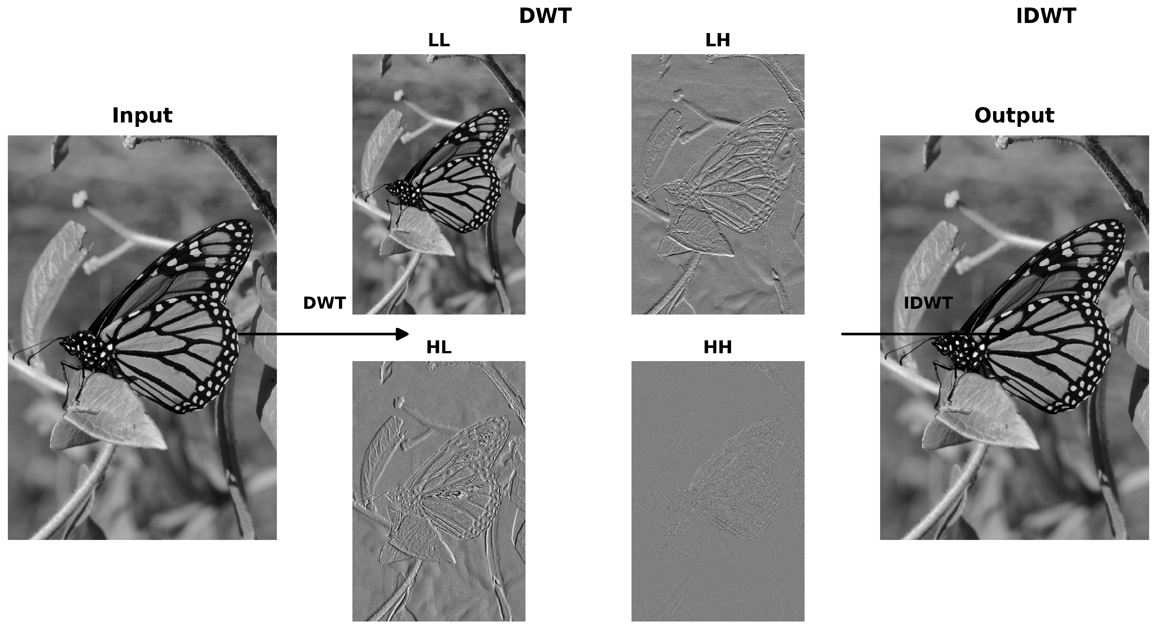
Figure 2.
U-Net architecture for biomedical image segmentation. The network consists of a contracting path for contextual feature extraction and an expanding path for precise localization through skip connections. Adapted from Ronneberger et al. [8].
Figure 2.
U-Net architecture for biomedical image segmentation. The network consists of a contracting path for contextual feature extraction and an expanding path for precise localization through skip connections. Adapted from Ronneberger et al. [8].
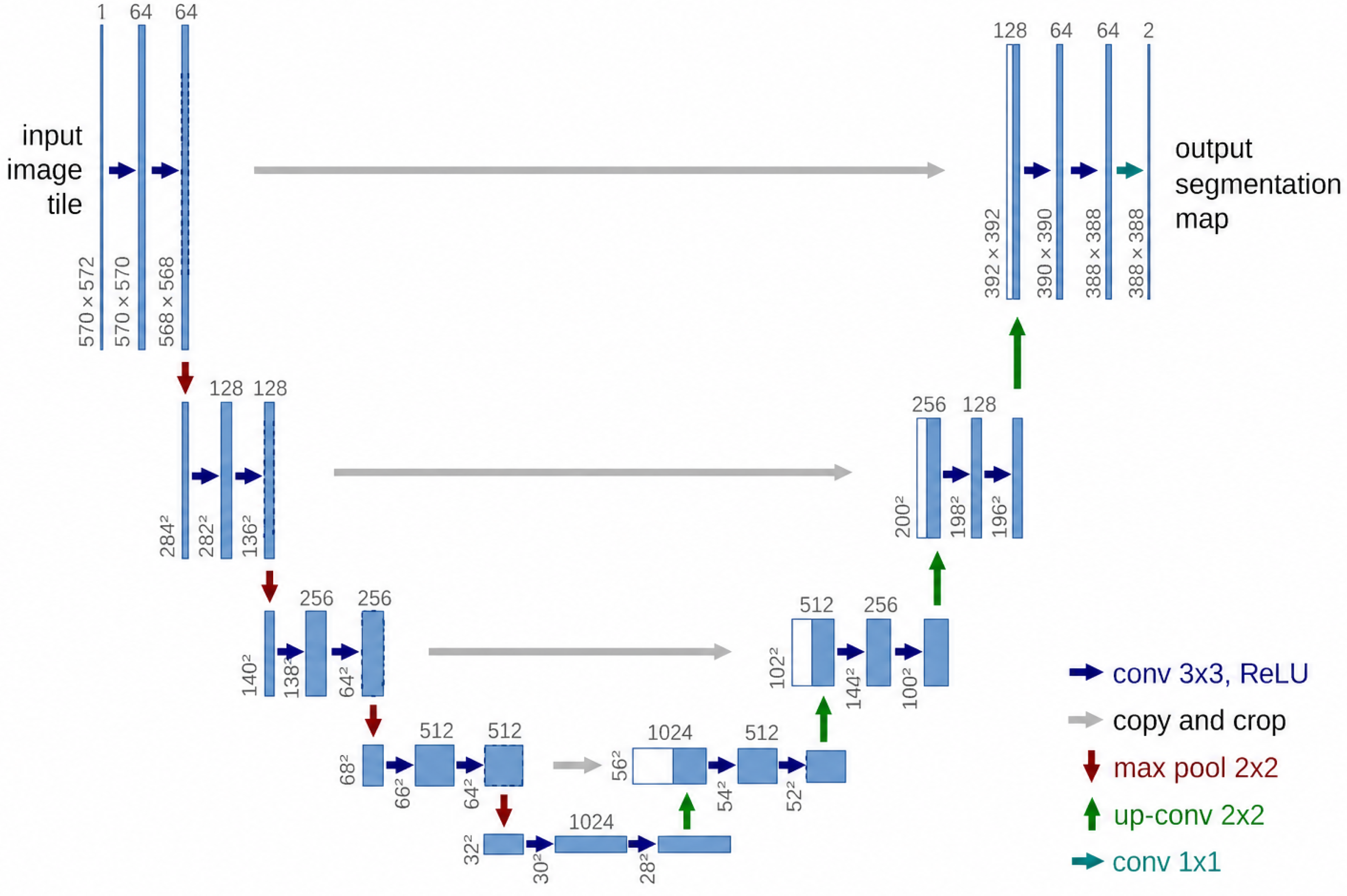
Figure 3.
Proposed wavelet-based U-Net methodology for super-resolution. The HR image is decomposed by DWT, only the LL band is retained and prepared as ll_norm and ll_raw, the Wavelet U-Net predicts missing high-frequency subbands , and the final SR output is reconstructed through IDWT.
Figure 3.
Proposed wavelet-based U-Net methodology for super-resolution. The HR image is decomposed by DWT, only the LL band is retained and prepared as ll_norm and ll_raw, the Wavelet U-Net predicts missing high-frequency subbands , and the final SR output is reconstructed through IDWT.
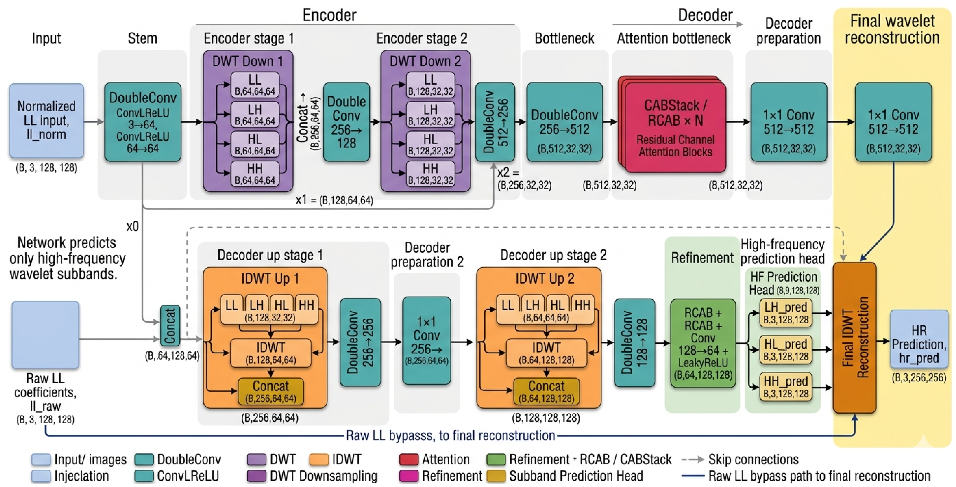
Figure 4.
Wavelet-based encoder using DWT to decompose input features into multi-scale sub-bands for downsampling.
Figure 4.
Wavelet-based encoder using DWT to decompose input features into multi-scale sub-bands for downsampling.
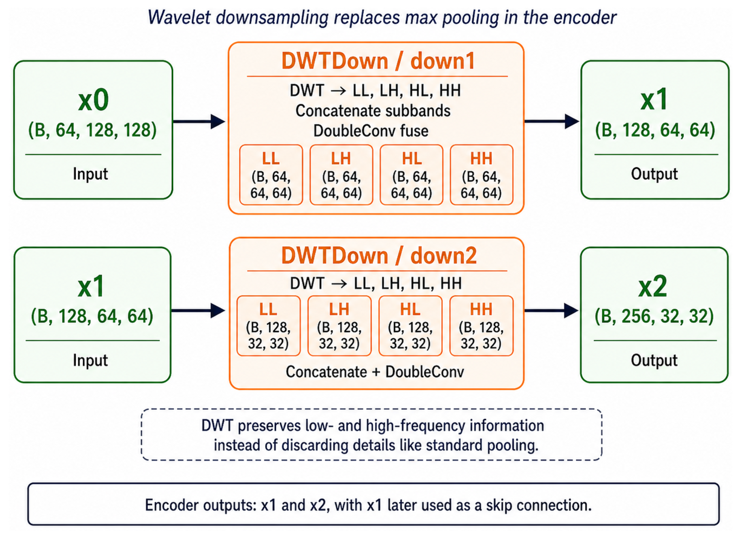
Figure 5.
Extended bottleneck module with double convolution and RCAB-based channel attention to enhance feature representation at the lowest spatial resolution.
Figure 5.
Extended bottleneck module with double convolution and RCAB-based channel attention to enhance feature representation at the lowest spatial resolution.
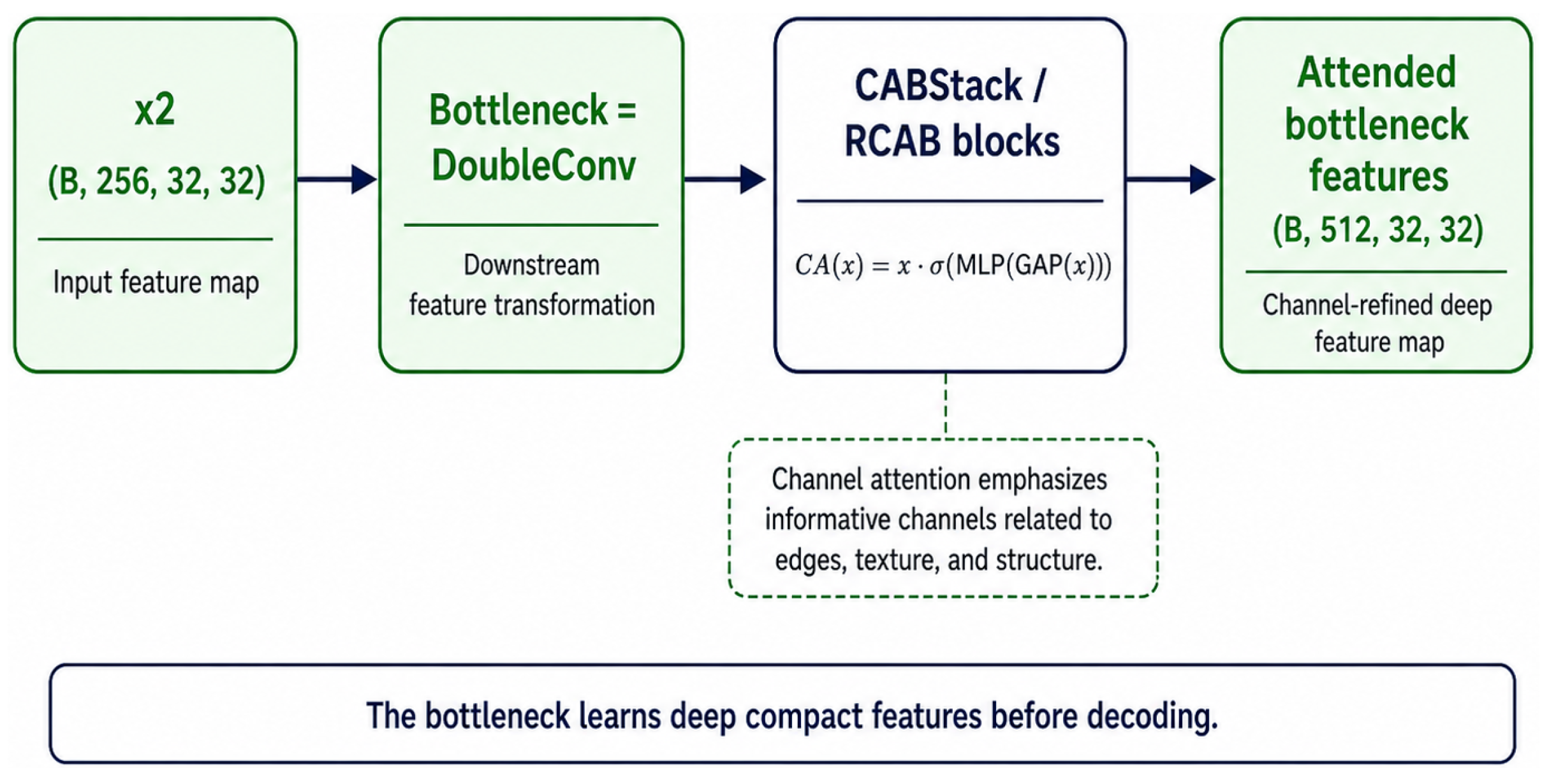
Figure 6.
Wavelet-based decoder using IDWT to progressively reconstruct spatial resolution from grouped feature sub-bands.
Figure 6.
Wavelet-based decoder using IDWT to progressively reconstruct spatial resolution from grouped feature sub-bands.
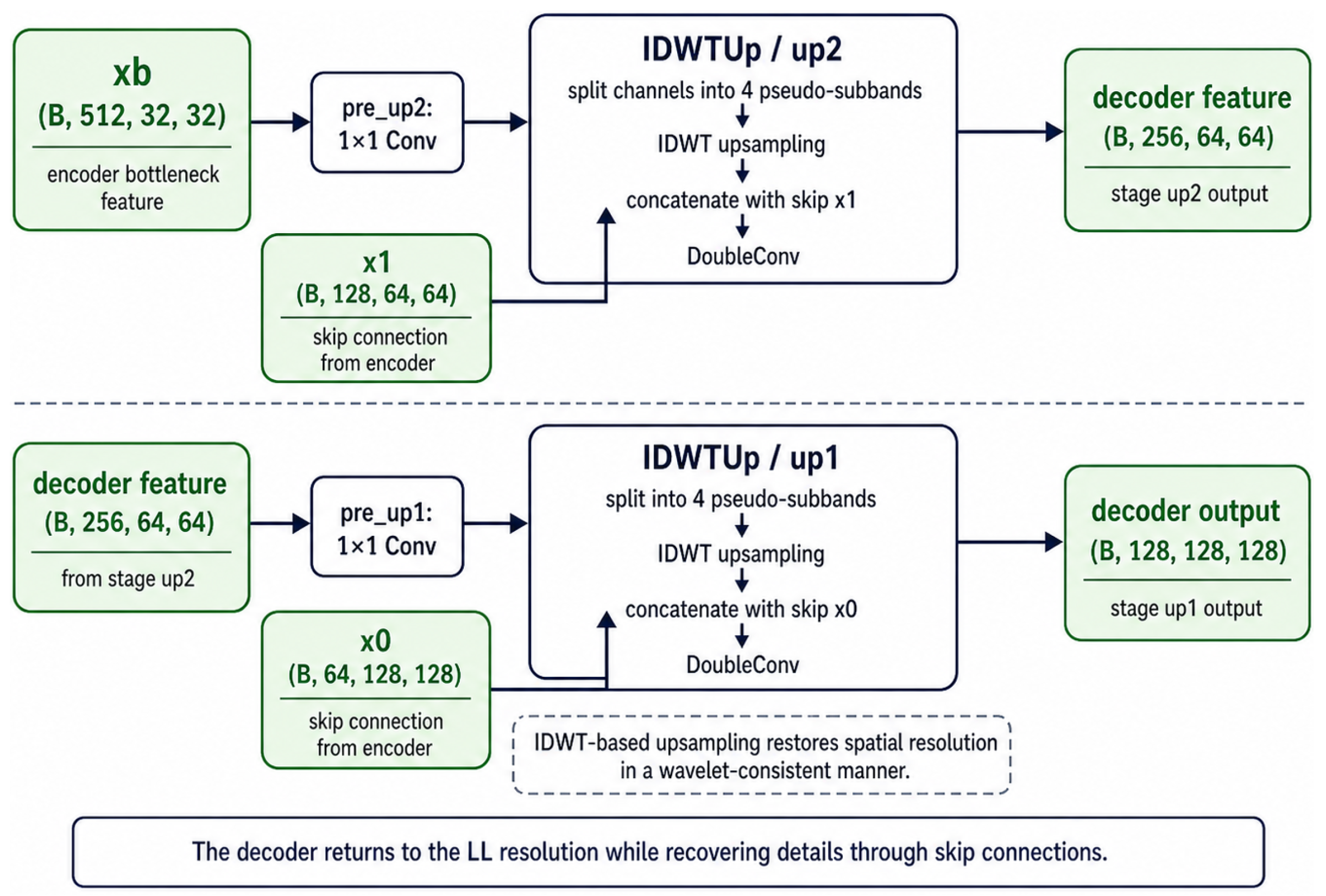
Figure 7.
High-frequency sub-band prediction head with RCAB-based refinement for generating detailed wavelet components.
Figure 7.
High-frequency sub-band prediction head with RCAB-based refinement for generating detailed wavelet components.
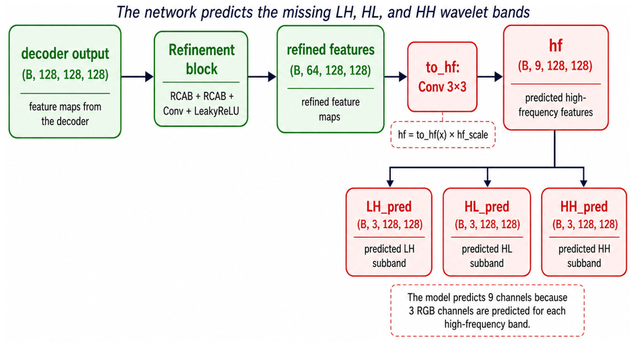
Figure 8.
Final high-resolution image reconstruction via IDWT by combining the original LR input with predicted high-frequency sub-bands.
Figure 8.
Final high-resolution image reconstruction via IDWT by combining the original LR input with predicted high-frequency sub-bands.
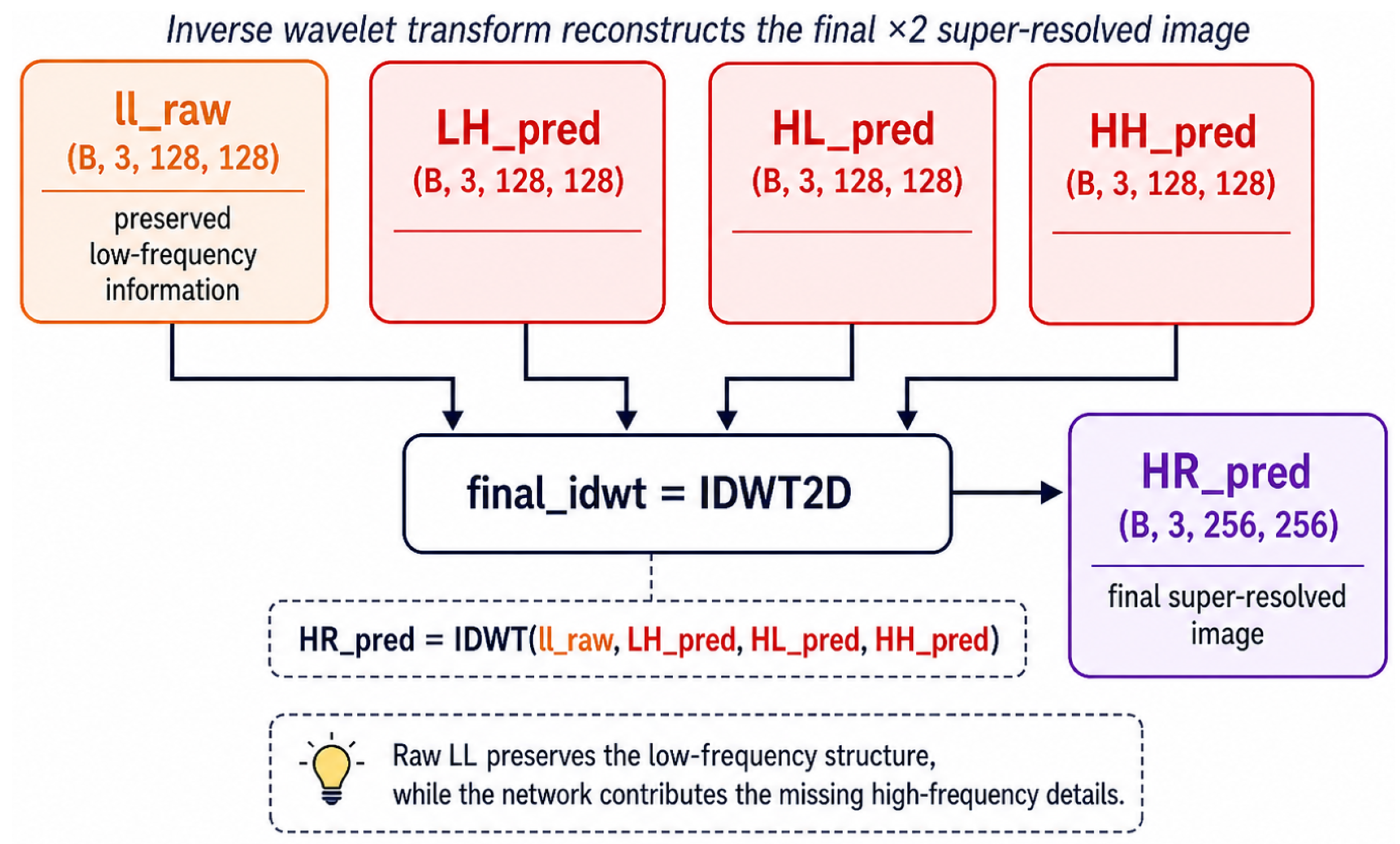
Figure 9.
Training convergence of the proposed DWT/IDWT U-Net on DIV2K and quantitative comparison against conventional upsampling baselines on Set5, Set14, and BSD100.
Figure 9.
Training convergence of the proposed DWT/IDWT U-Net on DIV2K and quantitative comparison against conventional upsampling baselines on Set5, Set14, and BSD100.
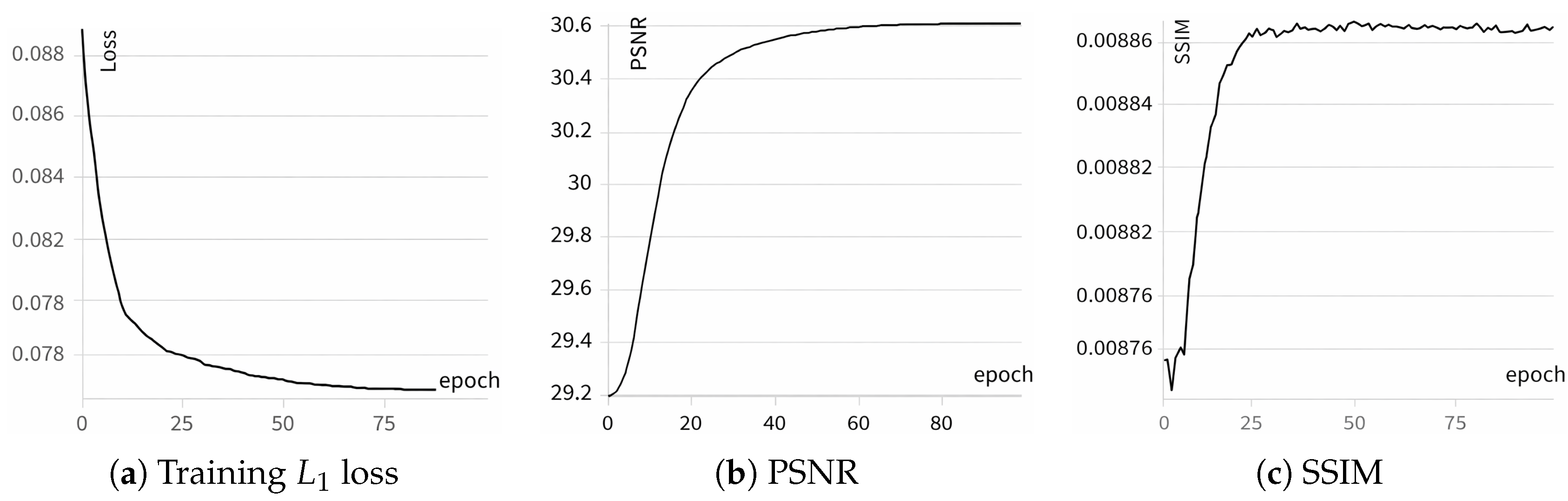
Figure 10.
Results comparison across U-Net variants with the proposed modification.
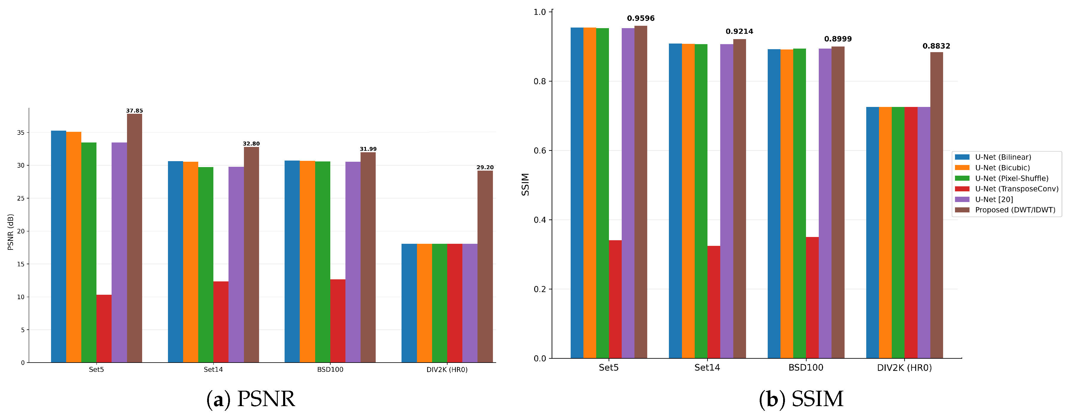
Figure 11.
Qualitative comparison on the people image. Top row: reconstructed images. Bottom row: magnified patches highlighting object boundaries and fine details.
Figure 11.
Qualitative comparison on the people image. Top row: reconstructed images. Bottom row: magnified patches highlighting object boundaries and fine details.
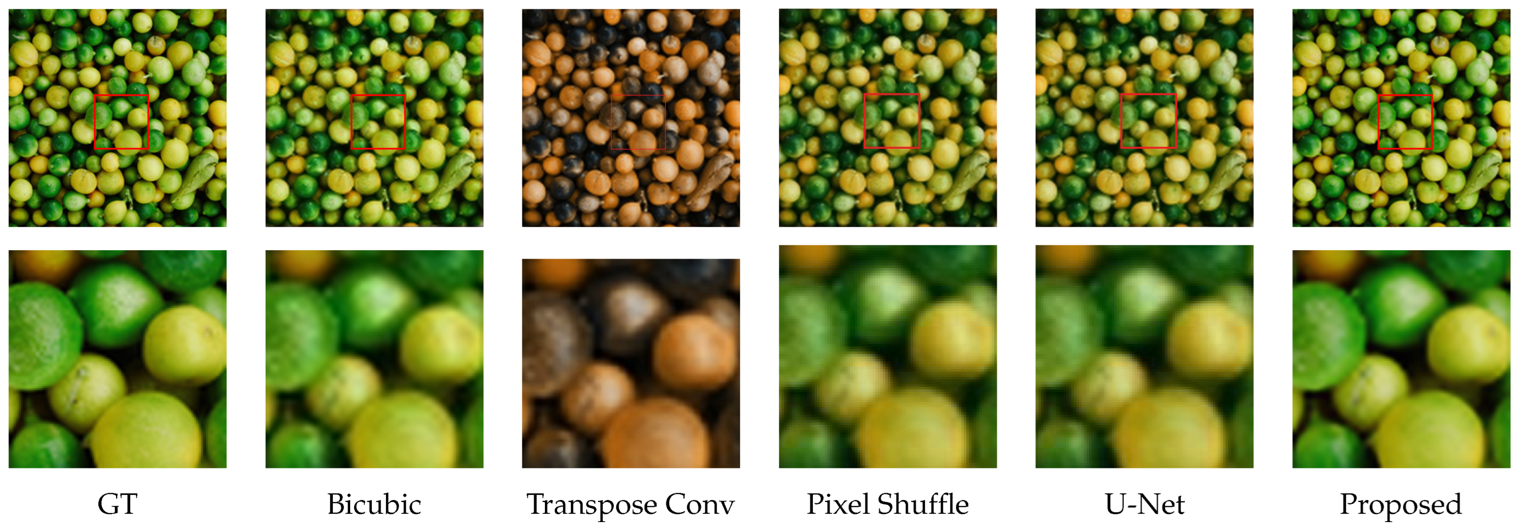
Figure 12.
Qualitative comparison on the flower image. Top row: reconstructed images. Bottom row: magnified patches highlighting texture and structural details.
Figure 12.
Qualitative comparison on the flower image. Top row: reconstructed images. Bottom row: magnified patches highlighting texture and structural details.
Figure 13.
Qualitative comparison on the people image. Top row: reconstructed images. Bottom row: magnified patches highlighting object boundaries and fine details.
Figure 13.
Qualitative comparison on the people image. Top row: reconstructed images. Bottom row: magnified patches highlighting object boundaries and fine details.
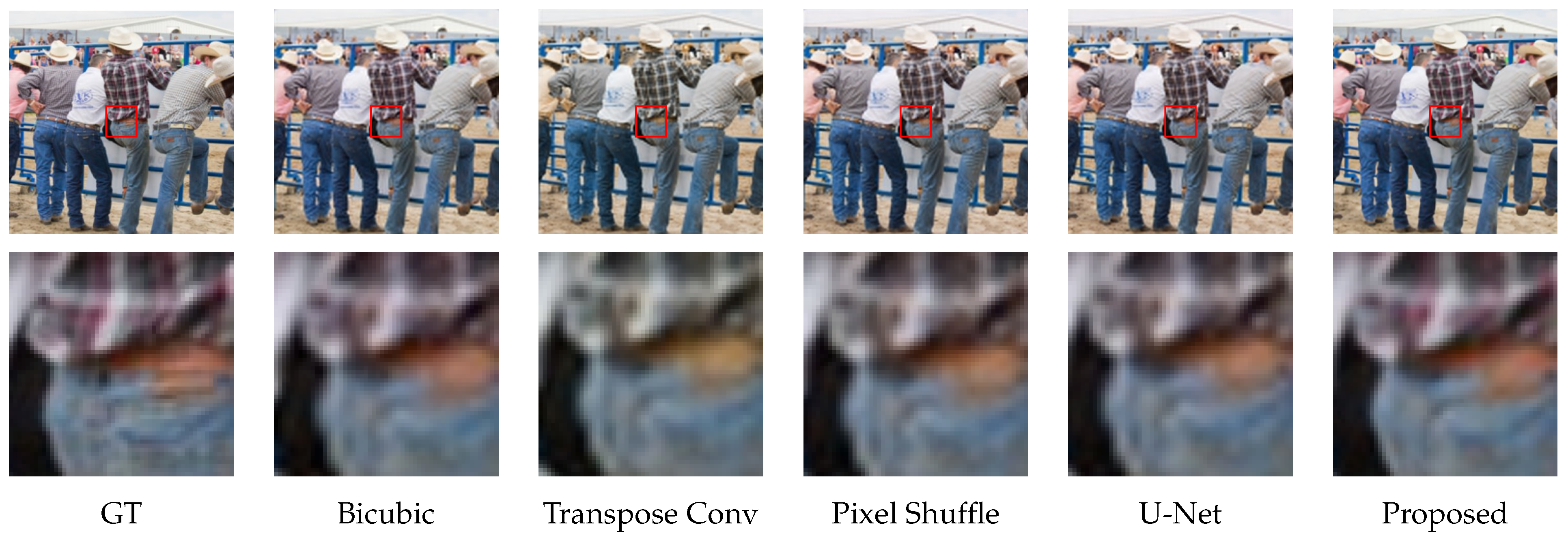

Table 1.
Comparative Summary of Super-Resolution Methods and Their Limitations.
| Ref Model | Year | Backbone | Upsampling | Freq. Aware | Limitation |
|---|---|---|---|---|---|
| SRCNN [17] | 2014 | CNN | Bicubic Pre-up | No | Pre-upsampling increases computational cost |
| ESPCN [22] | 2016 | CNN | Pixel-Shuffle | No | Sub-pixel rearrangement loses edge sharpness |
| VDSR [50] | 2016 | ResNet | Bicubic Pre-up | No | Prone to overfitting at increasing network depth |
| DRCN [18] | 2016 | Recursive CNN | Bicubic Pre-up | No | Slow convergence due to recursive weight sharing |
| DRRN [51] | 2017 | Residual | Bicubic Pre-up | No | High memory consumption during training |
| EDSR [19] | 2017 | ResNet | Pixel-Shuffle | No | Large model size limits practical deployment |
| LapSRN [20] | 2017 | Laplacian | Progressive | No | Multi-scale pyramid increases training complexity |
| RCAN [21] | 2018 | Channel Attention | Pixel-Shuffle | No | Heavy computation due to deep attention modules |
| All SR [16] | 2018 | Survey article | SR Approaches | No | Single image super-resolution |
| Edge GAN [39] | 2019 | GAN | Transposed Conv | No | Training instability and mode collapse risk |
| MSFFRN [52] | 2020 | Residual CNN | Pixel shuffle | No | Multi-scale fusion adds architectural complexity beyond simple residual designs. |
| DBPN [53] | 2020 | CNN | learned up sampling | No | More complex than simple feed-forward SR networks |
| WRAN [32] | 2020 | Lightweight CNN | IDWT | Yes | No sub-band adaptive weighting and limited to natural image SR without medical validation. |
| CRAN [26] | 2021 | CNN-based residual | Pixel-Shuffle | No | Less flexible for long-range dependency |
| Swin Transformer [24] | 2021 | Vision Transformer | SR heads | No | Local window attention little improves SR |
| Modified U-Net [44] | 2022 | CNN | Transposed convolution | No | No frequency awareness at all |
| ESRT [23] | 2022 | CNN + Transformer | Pixel-Shuffle | No | Designed to reduce memory/cost, but still trades off |
| CAT [54] | 2022 | Transformer | Pixel-Shuffle | No | Designed for general image restoration, the transformer is more computationally |
| Dense U-Net [47] | 2022 | CNN | PixelShuffle | No | Limited model long-range dependencies less effectively. |
| IESRGAN [45] | 2023 | CNN GAN | Convolution layers | No | Limited generalization and poor ×8 performance. |
| DWSR [42] | 2023 | U-Net | IDWT | Yes | High computational complexity and needs to be improved in real-time performance |
| IDM [49] | 2023 | Diffusion model | ICB continuous upsampling | No | Diffusion-based SR is typically computationally heavier and slower |
| HAT [40] | 2023 | Transformer | Pixel-Shuffle | No | Higher complexity and memory than lighter SR models |
| DAT [41] | 2023 | Transformer | Pixel-Shuffle | No | More computationally demanding than lightweight CNN SR |
| UFSRNet [38] | 2024 | U-shaped CNN | IDWT | Yes | Limited to face images and lacks adaptive attention for wavelet sub-bands. |
| effWicacy [43] | 2024 | U-Net | IDWT | Yes | Limited to drone/battlefield data and lacks adaptive per-sub-band weighting in the wavelet domain. |
| AdaFormer [48] | 2024 | Efficient Transformer | Pixel-Shuffle | No | Designed mainly for efficiency-speed tradeoff |
| ATD-SR / AST [25] | 2024 | Transformer | Pixel-Shuffle | No | More complex and heavier than lightweigh |
| DWTSRNet [29] | 2024 | SwinV2 Transformer | IDWT | Yes | Limited handling of noise and diverse image artifacts |
| WTMAFS/ [34] | 2024 | CNN | Pixel-Shuffle | Yes | Limited performance at high magnification with high resource cost. |
| DDSRNet [30] | 2025 | CNN with DWT | IDWT | Yes | Limited adaptability across diverse hyperspectral scenarios |
| vHeatSR [31] | 2025 | Vision model | IDWT | Yes | HCO struggles with long-range dependency learning |
| WFDRN [35] | 2025 | Transformer + CNN | Pixel-Shuffle | Yes | Hard-split dual-branch (Transformer for LF, CNN for HF) uses no learned adaptive weighting between branches |
| DWT-UNet [33] | 2025 | U-Net | IWT | Yes | All sub-bands are treated equally, limiting adaptive focus on high-frequency details crucial for super-resolution. |
| WT-GAN [37] | 2025 | GAN | DWT-based generator | Yes | Focused on label-map SR (not standard SR), with GAN instability and noise from weak labels. |
| GAN-based strategies [27] | 2025 | GAN-based + wavelet | GAN-based SR reconstruction | Yes | GAN-based SR can introduce hallucinated/artificial details |
| DSAUNet [46] | 2026 | U-Net + Transformer | Pixel-Shuffle | No | No frequency guidance, no medical validation, and state-of-the-art (SOTA) claim needs newer benchmark verification. . |
| HDP–CPP [36] | 2026 | Statistical Markov chain | Probabilistic estimation | Yes | Claim is relative to older statistical methods, not modern deep learning |
| Ours Wavelet U-Net | 2026 | U-Net + DWT | DWT / IDWT | Yes | We used a fixed family of wavelets like Bior4.4 |
Table 2.
Summary of the proposed Wavelet U-Net pipeline.
| Stage | Operation | Input | Output | Role |
|---|---|---|---|---|
| Preproc. | DWT on GT HR | Extract LR input and HF targets | ||
| Enc. 1 | DWT down | Feature downsampling | ||
| Enc. 2 | DWT down | Feature downsampling | ||
| Bottleneck | RCAB × 30 | Channel attention refinement | ||
| Dec. 1 | IDWT up + skip | Feature upsampling | ||
| Dec. 2 | IDWT up + skip | Feature upsampling | ||
| HF head | Conv 9ch | Predict LH, HL, HH | ||
| Reconstr. | IDWT | Final HR output |
Table 3.
Training hyperparameters.
| Item | Setting |
|---|---|
| Dataset | DIV2K |
| HR size | |
| Input | , |
| Optimizer | Adam |
| Learning rate | |
| Batch size | 8 |
| Epochs | 100 |
| Metrics | PSNR, SSIM |
Table 4.
Training and implementation details.
| Item | Configuration |
|---|---|
| Hardware | Single GPU (Google Colab L4, CUDA) |
| Framework | PyTorch with PyTorch Lightning |
| LR schedule | MultiStepLR; learning rate halved at epochs 60, 80, and 95 |
| Max epochs | 100 (early stopping patience = 15 on validation PSNR) |
| Precision | Mixed precision (16-bit automatic mixed precision (AMP)) |
| RCAB blocks | 30 |
| Evaluation Metric | PSNR, SSIM |
| Gradient clipping | L2 norm |
| Loss function | L1 loss + direct HF subband L1 |
| HF supervision | L1 loss between predicted LH/HL/HH and ground-truth subbands, averaged over the three bands |
| Exponential Moving Average (EMA) | Exponential moving average of generator weights (decay = 0.999); EMA weights used for validation |
| Seed | 42 |
| Checkpointing | Top-3 checkpoints by validation PSNR on Y channel (PSNR-Y), plus the last epoch |
Table 5.
Comparison of U-Net decoder variants for SISR. All models share the same base U-Net backbone and were trained on DIV2K under identical settings. Best results are highlighted in bold.
Table 5.
Comparison of U-Net decoder variants for SISR. All models share the same base U-Net backbone and were trained on DIV2K under identical settings. Best results are highlighted in bold.
| Variant | Down. | Up. | Set5 | Set14 | BSD100 | DIV2K-Test (HR0/LL-only) | ||||
|---|---|---|---|---|---|---|---|---|---|---|
| PSNR | SSIM | PSNR | SSIM | PSNR | SSIM | PSNR | SSIM | |||
| U-Net (Bilinear) | Strided Conv | Bilinear Interp. | 35.25 | 0.9548 | 30.64 | 0.9083 | 30.71 | 0.8915 | 18.08 | 0.7251 |
| U-Net (Bicubic) | Strided Conv | Bicubic Interp. | 35.09 | 0.9540 | 30.55 | 0.9071 | 30.68 | 0.8909 | 18.08 | 0.7251 |
| U-Net (Pixel-Shuffle) | Strided Conv | Pixel-Shuffle | 33.47 | 0.9525 | 29.74 | 0.9067 | 30.60 | 0.8937 | 18.08 | 0.7251 |
| U-Net (TransposeConv) | Strided Conv | Transpose Conv. | 10.31 | 0.3402 | 12.32 | 0.3243 | 12.68 | 0.3502 | 18.08 | 0.7251 |
| U-Net [8] | Max-Pooling | Up-Convolution | 33.49 | 0.9528 | 29.77 | 0.9068 | 30.56 | 0.8932 | 18.08 | 0.7251 |
| Proposed (DWT/IDWT) | DWT | IDWT + Learned HF | 37.84 | 0.9695 | 32.80 | 0.9296 | 31.99 | 0.9083 | 29.20 | 0.8832 |
Table 6.
Standard SR benchmark evaluation of the proposed method at scale.
| Data | N | HR0 PSNR | SR PSNR | Gain | HR0 SSIM | SR SSIM | Gain |
|---|---|---|---|---|---|---|---|
| Set5 | 5 | ||||||
| Set14 | 14 | ||||||
| BSD100 | 100 | ||||||
| Urban100 | 100 |
Table 7.
Quantitative comparison for super-resolution. The best and second-best results are highlighted in bold and underlined, respectively.
Table 7.
Quantitative comparison for super-resolution. The best and second-best results are highlighted in bold and underlined, respectively.
| Method | Scale | Set14 | BSD300 | ICDAR2003 | |||
|---|---|---|---|---|---|---|---|
| PSNR | SSIM | PSNR | SSIM | PSNR | SSIM | ||
| Bicubic [59] | 24.45 | 0.85 | 26.65 | 0.79 | 32.93 | 0.90 | |
| ESPCN [22] | 26.76 | 0.90 | 28.98 | 0.87 | 35.60 | 0.92 | |
| SRCNN [4] | 25.97 | 0.87 | 28.69 | 0.87 | 35.27 | 0.92 | |
| VDSR [60] | 28.66 | 0.93 | 29.39 | 0.88 | 36.23 | 0.94 | |
| EDSR [19] | 24.06 | 0.84 | 28.31 | 0.86 | 34.50 | 0.93 | |
| FSRCNN [61] | 23.13 | 0.81 | 28.75 | 0.87 | 35.05 | 0.94 | |
| DRCN [18] | 24.42 | 0.85 | 27.51 | 0.81 | 33.78 | 0.92 | |
| SRGAN [62] | 23.96 | 0.82 | 28.71 | 0.86 | 33.28 | 0.91 | |
| DBPN [53] | 28.41 | 0.92 | 29.87 | 0.88 | 36.23 | 0.94 | |
| UnetSR [44] | 26.72 | 0.87 | 29.42 | 0.88 | 35.71 | 0.94 | |
| UnetSR+ [44] | 28.40 | 0.92 | 29.84 | 0.88 | 37.37 | 0.97 | |
| Proposed Method | 32.80 | 0.93 | 32.30 | 0.91 | 37.74 | 0.96 | |
Disclaimer/Publisher’s Note: The statements, opinions and data contained in all publications are solely those of the individual author(s) and contributor(s) and not of MDPI and/or the editor(s). MDPI and/or the editor(s) disclaim responsibility for any injury to people or property resulting from any ideas, methods, instructions or products referred to in the content. |
© 2026 by the authors. Licensee MDPI, Basel, Switzerland. This article is an open access article distributed under the terms and conditions of the Creative Commons Attribution (CC BY) license (http://creativecommons.org/licenses/by/4.0/).
Copyright: This open access article is published under a Creative Commons CC BY 4.0 license, which permit the free download, distribution, and reuse, provided that the author and preprint are cited in any reuse.


