

Submitted:
03 July 2026
Posted:
06 July 2026
You are already at the latest version
Abstract
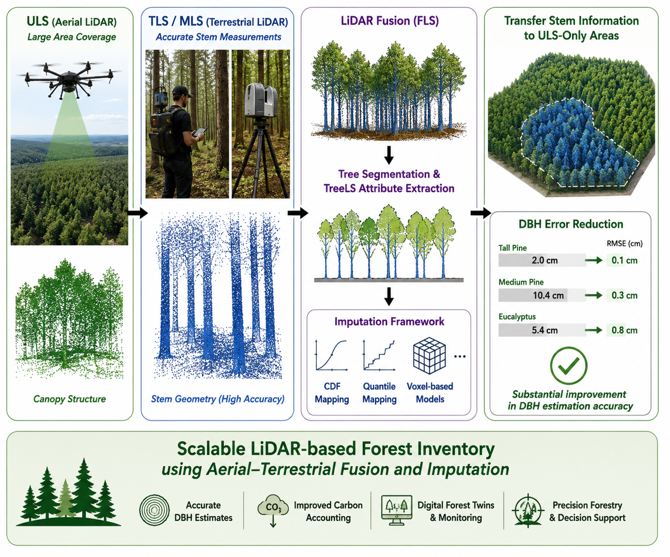
Forest inventory operations require accurate and scalable methods for estimating structural tree attributes such as diameter at breast height, tree height, and crown dimensions. Terrestrial laser scanning (TLS) and mobile laser scanning (MLS) provide detailed stem information but limited spatial coverage, whereas unmanned laser scanning (ULS) provides broad coverage but sparse internal stem structure. This study evaluates whether fused LiDAR point clouds and imputation-based correction methods can transfer accurate stem information from TLS, MLS, or fused calibration areas to larger ULS-only areas. ULS, TLS, MLS, and fused laser scanning (FLS) were analysed for 10 m and 20 m radiata pine, and 30 m eucalyptus stands. The TreeLS R package and regression-based methods were used for attribute extraction, and several imputation strategies were tested, including parametric cumulative distribution function (CDF) mapping, empirical and rank-based quantile mapping, conditional mean with residual spread restoration, and voxel-based imputation. The results show that TreeLS applied to TLS, MLS, and FLS produced substantially more reliable diameter at breast height (DBH) distributions than regression models applied directly to ULS data. For ULS-only areas, uncorrected regression estimates differed from field means by 2.0 cm for tall radiata pine, 10.4 cm for medium radiata pine, and 5.4 cm for mature eucalyptus. Using terrestrially trained voxel-based imputation reduced these differences to 0.1 cm, 0.3 cm, and 0.8 cm, respectively. Other distribution-aware imputation methods also substantially improved agreement with field-observed DBH distributions. These findings indicate that relatively small areas of high-density TLS or MLS or FLS data can be used to calibrate inventory estimates across larger ULS-only regions. The approach offers a practical compromise between the structural accuracy of terrestrial LiDAR and the spatial efficiency of aerial LiDAR, supporting scalable forest inventory estimation without requiring exhaustive terrestrial coverage.
Keywords:
remote sensing
; forest inventory
; LiDAR
; point cloud fusion
; unmanned laser scanning
; terrestrial laser scanning
; mobile laser scanning
; diameter at breast height
; voxel-based imputation
; forest structure
; tree segmentation
; precision forestry
; digital forest twins
1. Introduction
Forest inventory operations require systematic collection of structural information describing individual trees and forest stands to support sustainable forest management, timber valuation, carbon accounting, ecological monitoring, and operational planning. Accurate estimates of attributes such as diameter at breast height (DBH), total tree height (HT), crown dimensions, biomass, and stand density are fundamental to forest management and ecosystem assessment. However, traditional field-based inventory methods remain labour-intensive, time-consuming, spatially limited, and subject to observer bias and environmental constraints, particularly in structurally complex forests.
The need to characterise forest structure across spatial and temporal scales has intensified in recent years due to increasing interest in climate change mitigation, biodiversity monitoring, forest resilience, and carbon sequestration modelling. Forest structure strongly influences ecological processes including habitat complexity, hydrology, microclimate regulation, biomass accumulation, and disturbance dynamics. Consequently, accurate three-dimensional (3D) structural representation of forests has become a major focus of contemporary remote sensing research [1,2,3,4,5,6,7,8].
The internal structures of trees arise from a range of complex factors and interactions that influence both the growth and quantity of vegetation [9,10,11]. The complex nature of forests has proven challenging to measure accurately across scales and structure types [9,12]. There are also a variety of metrics ranging from traditional forest inventory approaches [13] to next-generation remote sensing techniques [14,15].
In recent decades, there has been a proliferation of remote sensing methods developed and applied to the task of quantifying forest structure, with a growing demand for fusing data collected from different sensors, platforms, and time frames [1,12,16].
LiDAR sensors generate highly accurate and detailed point clouds of forest structure from various viewpoints and are particularly useful when attempting to quantify tree structures. For instance, the detailed 3D structural data can be used to conduct inventory operations and to predict a range of phenomena, such as radio wave propagation [17], light interception [18], hydrology [19], microclimates [20], and resilience [21].
Terrestrial laser scanning (TLS) typically refers to statically mounted ground-based instruments that are particularly effective at capturing the fine-scale details of individual trees. Their mobile (terrestrial, handheld) counterparts are usually referred to as mobile laser scanners (MLS). MLS are much less time-consuming to operate and still provide clear, accurate, rapid, and high-resolution information about the complex internal features of tree structure beneath the canopy. This includes tree shape, size, branching patterns, and foliage density [22] (note: in this paper both terrestrial instruments are simply referred to as MLS, unless specifically noted otherwise).
Aerial laser scanning (ALS) refers to laser scanning obtained from manned aircraft and helicopters, and unmanned laser scanning (ULS) to laser scanning obtained from unmanned aerial vehicles (UAVs). ULS and MLS offer considerable potential relative to traditional field measurements in terms of improved accuracy and efficiency for describing forest stands. Such benefits materialise not only in terms of improved forest management practices, less fieldwork, repeatable and objective results, and greater safety, but also in terms of derived ecological outcomes. Each instrument has advantages and disadvantages in terms of point density, accuracy, spatial coverage, and occlusion by canopy constraining its capacity to obtain reflections from trees. Fusing ULS and MLS data allows the strengths of each to be leveraged to provide a better understanding of forest structure [23].
Despite these advances, significant challenges remain. ULS point clouds frequently lack sufficient stem density for reliable DBH reconstruction in dense forests, while MLS acquisitions remain operationally expensive over large areas. Moreover, the structural complexity of forests, species-specific stem morphology, canopy occlusion, and variability in laser acquisition parameters continue to limit the generalisability of many existing inventory approaches.
This study investigates whether, for a small increase in field trial effort (perhaps as little as 15 minutes), fusion of ULS and MLS point clouds, combined with voxel-based imputation and distribution-aware correction strategies, can overcome these limitations. Specifically, the study examines whether accurate stem attributes derived from MLS calibration regions can be transferred reliably to nearby regions observed only by ULS. The approach aims to preserve the structural accuracy of terrestrial LiDAR while leveraging the spatial scalability of aerial LiDAR, thereby enabling operationally practical forest inventory estimation across much larger areas than would otherwise be feasible using MLS alone.
The study’s approach was as follows: (i) ULS and MLS point clouds are fused into a single fused laser scanning (FLS) data set; (ii) accurate total tree height estimates are derived from the FLS; (iii) accurate stem attribute extraction tools are applied to the FLS; (iv) regression model attributes are extracted from the ULS component of the FLS; (v) the regression model estimates of the stem attributes are adjusted to match the accurate FLS estimates; and (vi) the corrected attribute model developed in the previous step is applied to the much larger section of forest observed only by the ULS.
1.1. Related Work
MLS has both proven to be very effective at quantifying components of tree structure [19,24,25,26,27,28,29,30,31,32,33,34]. MLS is commonly used in close-range, local area forest surveys, but they can present challenges when attempting to obtain information about the upper and outer canopy due to occlusion by intervening foliage [35,36]. It is also often difficult to get precise Global Navigation Satellite System (GNSS) signals in the forest, limiting the positional accuracy of such data sets and hence the derived tree location estimates [37,38].
ULS provide superior spatial coverage to MLS and efficient acquisition across large areas. However, ULS point clouds are generally less dense within lower canopy and stem regions due to canopy occlusion and their top-down viewing geometry. Consequently, while these systems are highly effective for characterising canopy structure [39,40,41,42,43,44,45] and terrain morphology [46,47,48], they are often less reliable for direct extraction of stem attributes such as DBH, particularly in dense or structurally complex forests [49,50,51,52,53].
ULS therefore measure forest and tree structure, but the accuracy with which this can be achieved depends on the orientation of the overstory [54], density and properties of the vegetation [55], and sensor’s data acquisition settings [56]. Dense foliage and complex understory pose challenges for accurately detecting and characterizing the vegetation beneath the canopy as the laser pulses attenuate through the upper canopy. So, while ULS provides valuable information about the upper canopy, its ability to capture detailed stem information remains somewhat limited.
Recent research [8,23,57,58,59] has increasingly focused on multi-platform LiDAR fusion approaches that combine the strengths of aerial and terrestrial sensing systems. FLS, which integrate ULS with MLS observations, provide complementary perspectives of forest structure from both above and beneath the canopy. This improves overall structural completeness, enhances point cloud registration accuracy, and increases the reliability of stem detection and attribute extraction. Fusion approaches also support emerging concepts such as forest digital twins and multi-scale structural modelling, where detailed local observations can be integrated with spatially extensive aerial data to improve forest characterisation across operational scales.
At the same time, advances in machine learning, voxel-based analysis, and point-cloud-driven modelling [60,61,62,63] have expanded opportunities for estimating forest attributes from structurally sparse LiDAR observations. Traditional approaches to DBH estimation typically relied on regression relationships involving tree height and crown dimensions calibrated against field observations. More recently, methods based on point cloud segmentation, stem reconstruction, voxel metrics, nearest-neighbour imputation, and distribution-aware statistical correction have demonstrated substantially improved performance, particularly when high-density terrestrial observations are available for calibration.
Most structural parameters were initially estimated using regression models based on HT and crown diameter, CD, and calibrated against ground-based observations [64,65,66,67,68,69]. More recently, new methods, largely based on MLS, have emerged that involve point cloud classification, tree segmentation, and stem reconstruction [14,15,70,71,72,73]. There is also a rich literature on modelling forest-level attributes, such as leaf area index, gap function, canopy cover, and the spatial distribution of trees [74,75,76], all obtainable from point clouds.
Imputation has also been used to leverage tree and forest attributes of interest [77,78,79]. Imputation is a non-parametric, multivariate modelling approach that aims to replace values of variables that are missing or have not been observed using measured samples of those that have. The imputed (replaced) values are based on the similarity between the values of predictor and target variables. The approach can be divided into direct and indirect methods [80,81,82,83,84,85,86]. Alternatively, variables may be measured using LiDAR and estimated using pixel or voxel-based metrics [42,86,87,88].
Imputation-based approaches are particularly attractive because they permit accurate structural information derived from small, high-quality MLS or fused calibration regions to be transferred to much larger ULS-only areas. Rather than requiring extensive field measurement campaigns or complete terrestrial coverage, imputation methods use structural similarity between observed and unobserved trees to infer missing inventory attributes. Recent developments in voxel-based metrics, empirical quantile mapping, rank-based distribution correction, and stochastic residual restoration further improve the ability of such methods to preserve realistic forest structural variability.
Fused point clouds also address several important operational limitations associated with individual LiDAR platforms. First, because aerial platforms are not affected by canopy-induced GNSS degradation to the same extent as MLS systems, fusion improves coordinate registration accuracy for MLS point clouds. Although MLS often provides sufficient point density for accurate stem reconstruction and tree characterisation, the absolute positional accuracy of tree locations may be poor due to degraded GNSS solutions beneath the canopy. ULS point clouds, by contrast, generally possess more reliable coordinate registration due to unobstructed GNSS reception and access to differential correction services.
Second, although ULS point clouds benefit from improved coordinate accuracy, the internal stem and branch structure represented within aerial point clouds is substantially sparser than that observed from MLS [59]. This often produces noisier estimates of stem geometry and poorer tree localisation performance, particularly in dense stands such as radiata pine. Fusion therefore provides both accurate georeferencing and improved fine-scale structural representation, enhancing stem detection and characterisation performance.
Third, fused point clouds provide structural observations from both above and within the forest canopy, improving representation of complex internal and external canopy structure. In addition to improving inventory estimation, this additional structural detail supports improved modelling of processes such as radio wave propagation, light interception, hydrology, microclimates, and forest resilience.
Finally, ULS–MLS fusion provides an opportunity to overcome one of the major limitations of LiDAR-based inventory operations: the need to balance the high structural fidelity but limited coverage of MLS against the extensive spatial coverage but reduced stem detail of ULS, without resorting to prohibitively large and time-consuming field campaigns.
2. Materials and Methods
Overall, the study prioritised an operationally realistic workflow over exhaustive parameter optimisation. While this supports practical relevance, it also means that some acquisition and processing choices—such as ULS flight speed, LiDAR sensor configuration, morphological filtering parameters, and regression model transferability—were not independently optimised or subjected to full sensitivity analysis.
Future studies should systematically vary these parameters and quantify their effects on tree detection, height estimation, crown delineation, DBH extraction, and imputation accuracy. This would allow the relative contributions of sensor performance, acquisition design, processing choices, and biological variation to be separated more clearly.
2.1. Trial Sites, Equipment, and Data Collection
The study relies on 3D MLS and ULS point clouds obtained for two radiata pine (Pinus radiata) plantations in South Australia and two plantations of eucalyptus (Eucalyptus globulus and Eucalyptus sieberi) in Tasmania. The data sets were fused and DBH, HT, and CD compared to traditional field measurements. Comparisons of tree structure and stem location estimates for the individual and fused point clouds are reported elsewhere [23].
South Australian Site: The South Australian trial site was within the Mount Crawford Forest, which is located approximately 46 km northeast of Adelaide, South Australia in the northern region of the Adelaide Hills. Covering over 12,000 ha and managed by ForestrySA, a state-owned corporation charged with the commercial management and conservation of the South Australian government’s native forest and commercial pine plantations, the Mount Crawford Forest is characterised by gently undulating terrain.
The specific test site, known as Goat Farm, comprised two parcels of planted radiata pine (Pinus radiata), located around the crossroad at 34° 42’ 54.5” S, 139° 1’ 38.7” E. This site was selected as a representative example of pine plantation and included regions of young-age (10-year-old) and mature (19-year-old), mid-rotation trees. The terrestrial data sets reported in this study were obtained in March 2024 and the aerial data set and field observations (both taken on the same day) in May 2024. Both dates fall in local autumn, a slow growing period for radiata pine.
The overarching data acquisition strategy was to roughly match the operational effort required for the aerial and terrestrial systems (set-up and take-down time for both systems were roughly equivalent, with similar battery charging requirements). In other words, the goal was to gain insight into the (approximate) relative operational utility of each instrument rather than the best possible outcomes. Thus, although two aerial data sets were collected (one high density, the other low), the overall duration of the longer flight was limited to around 25 minutes (one drone battery charge), whilst the faster flight was limited to around 10 minutes, matching the duration of the terrestrial observations.
ULS Data Acquisition: The ULS used for this study was a Zenmuse L1 LiDAR/camera unit mounted on a DJI Matrice 350 (M350) drone (www.dji.com). The LiDAR collected data in triple return mode at a sampling rate of 160 kHz. The manufacturer states an accuracy of 10 cm horizontal and 5 cm vertical for a measuring distance of 50 m. A built-in camera provided red-green-blue (RGB) information for each point, enabling colourised scene reconstruction. The point clouds were generated using the DJI Terra software (www.dji.com).
The M350 carries a navigation system capable of a real time kinematic (RTK) carrier phase differential global positioning system (DGPS) solution, which may be used in conjunction with corrections associated with a first order geodetic control network. The absolute location of the M350 at any moment is cited as ± 0.1 m (www.dji.com).
The M350 was flown in a standard lawnmower pattern over the tree plots at an altitude of 60 m above ground level. The distance between opposing legs of the lawnmower paths was about 50 m. Two data sets were taken: one using a forward speed of about 5 m/s, the other 10 m/s, both with 50% side overlap. The resultant point clouds comprised around 1,900 and 2,300 points/m2, respectively.
MLS Data Acquisition: The MLS was a hand-held GeoSLAM Zeb-Horizon with a 360° x 270° field of view (www.geoslam.com). The manufacturer cites vertical and horizontal angular resolutions of the unit as 2° and 0.2°, respectively, with a sampling rate of 300,000 points/s. The range accuracy is cited as 6 mm. The point clouds were generated using the GeoSLAM Connect V2 software and the cited relative accuracy of the data was 6 mm (www.geoslam.com).
The MLS Connect software uses a process known as simultaneous localization and mapping (SLAM) [89]. As its name suggests, SLAM maps an area while simultaneously keeping track of the location of the sensing unit within that map. For SLAM to provide an undistorted point cloud, the operator of the MLS must ‘close the loop’, i.e., return to a previously visited location, usually the commencement points of a track. Experience has shown that, for accurate results, loop closure should occur within about 10 minutes of track commencement. All MLS data sets were obtained by commencing walked tracks outside each tree plot and, upon entering them, marching up and down rows of trees before returning to the start point within 10 minutes.
These acquisition and processing parameters, including ULS flight speed, sensor configuration, and morphological filtering window size, were selected to reflect operationally realistic survey conditions rather than exhaustive optimisation. The flight speeds were chosen to approximate practical field deployment constraints, including battery duration, area coverage, and repeatability, while still maintaining point densities suitable for canopy-scale structural extraction.
Field Observations: In addition to the LiDAR scanning, field observations of HT, DBH, and CD were also made using traditional techniques. A total of 95 trees were measured. These comprised four sets of 20 trees—two sets within the tall plot, two within the medium—with an additional 15 trees also measured in the tall tree plot. Two sets of 20 trees were in regions observed by the MLS and ULS (one in the tall trees, the other in the medium) and two were in the region observed only the ULS (again, one in the tall trees, the other in the medium). An additional 15 trees measured in the tall trees were located within the MLS-observed region. Henceforth, these small subsets will be referred to as the “MLS-observed trees” and “ULS-only tree sites”. All field observations were obtained in May 2024, on the same day as the high-resolution ULS data.
Tasmanian Site: In addition to the radiata pine observed at Mount Crawford, experiments were also conducted at a forestry stand located in southern Tasmania near the township of Cradoc. The site, which is owned by Reliance Forest Fibre, is at 43° 6’ 27.6” S, 147° 4’ 28.7” E. The site was chosen because of its proximity to three differently aged coupes that provided a variety of tree height environments in which to test the performance of the GNSS receiver. Tree types include 3-year-old Tasmanian blue gums (Eucalyptus globulus) with a maximum height of around 6 m and 22-year-old silver top ashes (Eucalyptus sieberi) with heights of approximately 35 m.
ULS Data Acquisition: Two flights were undertaken over the trial site, both using a DJI Matrice 350 drone. The first flight used a DJI Zenmuse L1 LiDAR, the second a DJI Zenmuse L2 LiDAR. The point cloud densities derived from the L1 and L2 were estimated as 2,100 and 9,500 points/m2, respectively (Table 1). Differences between the L1 and L2 sensors should be interpreted cautiously, as observed performance differences may reflect both sensor capability and acquisition geometry rather than sensor type alone.
Positioning accuracy for the ULS data was achieved using the DJI differential (carrier phase) real time kinematic (D-RTK) GNSS base station that supplied real time navigation corrections to the M350 drone whilst in flight. The D-RTK was set up over an accurately surveyed point using HxGN SmartNet (https://hxgnsmartnet.com/), allowing the ULS data to be tied into a local survey network. Flights were conducted at a forward speed of 3 m/s and height of 50 m above ground level. They used terrain follow mode to maintain a roughly constant ground sample distance (GSD). The flights primarily covered the triangular wedge of tall trees, which were concurrently scanned with a TLS.
TLS Data Acquisition: The TLS data was collected using a 1.3 m tripod-mounted Leica Nova MS50 multi-station LiDAR (www.leica-geosystems.com), which can scan at 1,000 Hz and has an accuracy of 1–2 mm. Three surveyed points were used as reference for the MS50 so that the TLS data could be tied into the local survey network. The raw TLS contained 1.1 billion points.
Field Observations: Field observations of DBH were also made using traditional techniques about three months after the ULS and TLS data were collected. Observations from 22 trees were collected for this site.
2.2. Methods
FLS Point Cloud Fusion: When fusing individual point clouds, the key goal is to find an accurate spatial transformation that establishes correspondence and alignment, usually for the less-accurately established MLS data set with that observed above the canopy by the ULS. Point cloud fusion plays a major role in many applications, including vegetation modelling [72], change and object detection [90,91], robotics [92], and classification [93]. There are three common approaches to point cloud fusion: auxiliary-based, point-based, and feature-based [94], with several techniques that rely on the effective detection of tree positions [95,96,97,98,99,100].
While some of these methods have been developed for point cloud fusion in forest environments, they predominantly address limitations and characteristics of small regions, focusing on the MLS point clouds. More recently, a few methods that focus on fusing point clouds obtained from aerial and ground-based platforms have been proposed [101,102,103,104,105], but they usually rely on initial position estimates of individual trees being obtained using GNSS receivers, known tree attributes, or the pre-identified geometry of the ULS and MLS point clouds.
The method used in this study relied on image processing to establish coarse correspondence between the ULS and MLS canopy height models (CHM), followed by fine registration using the ICP algorithm. First, the ULS and MLS data sets were separated into ground and non-ground points using a morphological filter. The filter comprises three steps: (i) creation of a minimum elevation surface map (MESM); (ii) segmentation of this map into ground and non-ground elements; and (iii) conversion of the original point cloud data into a canopy height map. The process is depicted graphically in Figure 1.
The morphological filter first rasterised the point cloud within the horizontal (x-y) plane, noting the lowest elevation value for each raster element. These minima are combined to create a MSEM and an ‘opening’ operation is carried out on the MESM. The slope between the MSEM and opened surface is calculated and, if the difference is less than 0.15, the point is categorised as ground. This operation is carried out iteratively, with the window radius increased by 0.1 m per iteration until it reaches a maximum radius of 2 m. The result is a binary mask in which each element in the point cloud is classified as either ground or non-ground. Ground points are then used as the basis for a Delaunay triangulation interpolation [106] in which the sample points are the x-y locations of each point. Finally, the surface created by interpolation is differenced from the original height (z-axis) values of the point cloud to create a topographically level point cloud. CHM were obtained by converting each levelled point cloud into a set of 5 cm voxels and identifying the uppermost cell in each vertical column of the 3D raster.
The morphological filtering parameters were selected empirically to provide stable ground/non-ground separation across the trial sites. The progressive window radius was intended to remove local terrain variation while preserving tree-scale structure. However, no formal sensitivity analysis was undertaken, and future work should quantify the influence of filtering window size on canopy height models, tree segmentation, and derived structural attributes.
Next, the CHMs were converted to grayscale images and phase correlation [107] used to compute the geometric 2D transforms required to coarsely align the two 2D images before an iterative closest point (ICP) algorithm [108,109] is used to refine the alignment. Unlike several other techniques [95,96,97,99,110,111,112], the accuracy of this approach does not depend upon accurate determination of tree positions or having complete trees in both scenes. Moreover, the technique enables use of the GeoSLAM Zeb-Horizon unit (which does not contain an integrated GNSS) without the need for accurately surveyed ground control points (GCP). That is, the coordinates of the MLS point cloud can initially be computed relative to an arbitrarily selected origin and set of axes. This minimises operational field effort, as only the start points of the walked path need to be coarsely surveyed using GNSS.
As the point clouds were both pre-normalised to level ground and only coarse alignment is required, there was no requirement to translate the data in the z-axis (up) or rotate it about the x- or y-axes (east or north). The ULS point cloud was fixed as the target and the coarsely transformed MLS point cloud accurately matched to this target using the ICP algorithm. ICP iteratively estimates the translation and rotation needed to minimise the sum of squared differences between the coordinates of matched point pairs. Once accurately geo-registered, the point clouds were concatenated to form a single fused point cloud. The location accuracy of the ULS points (largely based on navigation solution of the real time kinematic differential GNSS receiver onboard the M350) is 10 – 20 cm [23].
Attribute Extraction: We estimated HT, CD, and DBH using two approaches: one simple (so it could be applied to poorly structured internal detail typical of the ULS data sets), and the other more sophisticated (with the intention of using it to accurately interpret the complex tree stem detail offered by the MLS and FLS data sets).
The simple approach used local density times intensity maps (LDTIM) to detect tree stems. LDTIM is effective for ULS point clouds of dense forest vegetation, such as radiata pine, when LiDAR penetration to the tree stems is relatively sparse.
Point density is typically highest in the vicinity of tree stems, which also tend to exhibit stronger LiDAR return intensities than surrounding canopy elements. Accordingly, the number of returns within each vertical column associated with a raster cell was summed to generate a point-density model, while mean relative intensity values were calculated by averaging the intensity returns within the same columnar structure. The normalised density and intensity layers were then multiplied to produce a local density–intensity map, and a Gaussian smoothing filter was applied using a 5 × 5 kernel with a standard deviation of σ = 1 (FWHM ≈ 2.36 pixels).
It is acknowledged that the intensity measurements obtained from the L1 and L2 sensors were not radiometrically calibrated to account for range, incidence angle, or other acquisition-related effects. Consequently, absolute intensity values may vary across the flight strip. However, the proposed method relies primarily on relative intensity contrasts within local neighbourhoods rather than absolute intensity magnitudes. As a result, the combined density–intensity metric remained effective for identifying stem locations despite the use of uncalibrated intensity data.
Individual tree crowns were segmented using a marker-controlled watershed algorithm [113] applied to the complement of the canopy height model. Tree-top detections were imposed as regional minima, and watershed segmentation then performed using 8-neighbour connectivity. Segments with canopy heights below a threshold of 1 m were removed, and very small segments containing fewer than 6 pixels discarded before re-labelling the remaining tree crowns sequentially.
CD was estimated by calculating the crown area associated with each tree and converting this to an equivalent circular diameter. Allometric models, implemented as regression-based relationships linking HT, CD, and DBH, for eucalyptus globulus and pinus radiata were then applied. The model, written as DBH = exp(β0+β1 ln(HT)+β2 ln[π(CD/2)2]) [68], was based on a large Chilean plantation data set and reported strong fits for DBH estimation, with adjusted R values generally in the range of approximately 0.93 – 0.98 depending on species and predictor set. It was preferred over those of [66,114,115,116,117], which reported larger errors. Models that included tree density (e.g., [69]), were left for future work.
Stem Imputation Modelling: Use of FLS and MLS improves attribute extraction relative to ULS. However, such data sets are limited by the MLS plot size. Moreover, regression models, often the only viable approach for extracting stem parameters from sparser ULS point clouds, are often inadequate for commercial inventory operations.
To obtain better estimates of stem attributes in the region observed solely by the ULS, we: (i) applied the TreeLS R package to the FLS (and MLS) data sets to extract DBH; (ii) compared the outcomes of (i) to the LTDIM and regression model estimates of DBH for the same trees obtained using just the ULS component of the FLS data set (referred to as FLS_ULS data); (iii) adjusted the FLS_ULS regression model estimates of DBH to match the accurate (TreeLS) estimates; and (iv) applied the corrected model developed in step (iii) to the much larger section of forest observed only by the ULS alone (referred to as ULS_ALL data). The TreeLS parameters used for each tree group are shown in Table 2.
Several detailed correction strategies were considered. However, all rely on the same basic assumption: that the distribution of stems within the FLS zone is broadly representative of those in ULS_ALL. In operational terms, this would mean selecting a region (or regions) observed by the MLS on this basis, perhaps using the ULS data set as a primer.
Direct Adjustment of Regression Model (Strategy 1): Empirical relationships between TreeLS estimates of DBH (derived from the FLS point cloud) and estimates of HT and CD (derived from LTDIM applied to the FLS_ULS data) were fitted to the regression model pertinent to each forest type/species so that model coefficients could be estimated using nonlinear least-squares optimisation. The data was first filtered to retain only trees with valid DBH, height, and crown measurements prior to model fitting. DBH for ULS_ALL data was then predicted using both HT and CD as explanatory variables based on the adjusted coefficients. During prediction, tree height and crown diameter values were constrained to biologically realistic ranges derived from the training data to reduce extreme extrapolation behaviour.
Weighted Adjustment of Regression Model (Strategy 2): In this strategy, model coefficients were again estimated using nonlinear least-squares optimisation, but with a 90% weight towards the original coefficients of [68]. The training data was again filtered to retain only trees with valid DBH, height, and crown measurements prior to model fitting. Prediction constraints to biologically realistic ranges to reduce extreme extrapolation behaviour were not required for this approach.
CDF with Two Beta Functions (Strategy 3): In this strategy, the DBH for each tree within FLS was computed using TreeLS and a beta distribution, , fitted to this data, where is the sample data and the CDF value associated with each DBH value, .
A probability distribution function (PDF) is a statistical means to describe the likelihood a random variable takes a particular value. A CDF describes the distribution of random variables with the advantage that it can be defined for any kind of random variable (discrete, continuous, and mixed). A CDF is derived by cumulatively summing the PDF and may be uniquely inverted. The goal of the imputation strategies is thus to adjust the CDF of the FLS_ULS regression model to match the TreeLS estimates and then apply the corrections to the ULS_ALL region that can only have regression models applied. The inverse of the corrected CDF may then be used to compute better attribute values for this (larger and sparser) region.
LDTIM was used to determine the location of every tree in the ULS_ALL data set and the regression model of [69] used to calculate their corresponding DBH values. A second beta function, , was fitted to this data set and the CDF values, , again calculated for each of the regression estimates of DBH, . Using the distribution, the inverse values of the distribution probabilities were then evaluated at each CDF value of the ULS_ALL regression estimates used to form (i.e., ), so , where are the imputed values for the ULS_ALL data set.
CDF with Other Functions (Strategies 4 – 7): In these strategies, the beta functions were simply replaced by Weibull, Nakagami, Normal, and Log-Normal distributions, and the imputation processing repeated.
Empirical Quantile Mapping (Strategy 8): In this strategy, empirical quantile mapping [118] was used to adjust the distribution of predicted DBH values so that they more closely matched the distribution of TreeLS reference DBH observations. The method first calculated empirical quantiles for both the predicted DBH distribution and the reference DBH distribution. A mapping relationship was then established between equivalent quantiles in the two distributions. Predicted DBH values were subsequently transformed using interpolation between these matched quantiles. This approach preserves the relative ordering of imputed trees while correcting systematic distributional differences such as mean bias, variance compression, skewness, and under- or over-estimation of large trees. Unlike additive or multiplicative scaling, empirical quantile mapping adjusts the full distribution of predictions and thus improves agreement across both small and large diameter classes.
Rank-Based Quantile Mapping (Strategy 9): In this strategy rank-based quantile mapping [119] was used to adjust predicted DBH values so that their statistical distribution more closely matched the reference DBH distribution derived from training observations. The method first ranked all predicted DBH values from smallest to largest. Equivalent ranks were then identified within the reference DBH distribution. Each predicted value was subsequently reassigned according to the corresponding reference quantile. For example, a tree predicted to lie at the 90th percentile of the predicted distribution would be mapped to the 90th percentile of the reference DBH distribution. This preserves the relative ordering of trees while correcting systematic distributional differences between predicted and observed values.
This approach is particularly effective when predictive models reproduce relative tree ordering well but compress or distort the spread of DBH values. By aligning empirical quantiles between predicted and reference distributions, the method restores realistic stand-level DBH variability while maintaining the spatial and structural relationships learned by the predictive model.
The predictive models generated by rank-based quantile mapping generally preserve relative DBH ordering well, while underestimating distributional spread. The rank-based approach therefore restored realistic stand-level variability without requiring strong assumptions about the exact functional form of the distributional correction. Moreover, unlike direct mean correction (see below), rank-based quantile mapping adjusts the entire distribution simultaneously, including mean structure, variance, skewness, and upper and lower distribution tails.
Conditional Mean with Residual Spread Restoration (Strategy 10): In this strategy, the conditional mean with residual spread restoration approach [120] was used to generate DBH predictions that preserved both the expected structural relationship between predictor variables and the natural variability observed in the training data.
In the first stage, a predictive model was trained using matched FLS–TreeLS observations. The model estimated the conditional mean DBH for each tree based on structural predictor variables derived from voxel and canopy metrics. This produced a smooth expected DBH estimate representing the average relationship between predictor variables and DBH. However, mean predictions alone tend to compress variability and underestimate the natural spread of tree diameters within a stand. To address this, residual spread restoration was applied in a second stage. Residuals from the training data (observed DBH minus predicted DBH) were sampled from structurally similar trees identified using approximate nearest-neighbour matching in predictor space. These residuals were then added back to the conditional mean predictions.
This process restored realistic heterogeneity in the predicted DBH distribution by preserving local variability, stand-level variance, upper and lower distribution tails, and nonlinear structural differences between trees. The resulting imputed DBH values therefore retained both the large-scale predictive trends learned from the training data, and the fine-scale stochastic variation characteristic of real forest structure.
Voxel-Based Imputation (Strategy 11): The final strategy, voxel-based imputation, was used to estimate DBH from structural information contained within the point cloud, rather than relying directly on TreeLS circle fitting for every target tree.
First, each tree’s point cloud was divided into a 20 cm voxel representation using a tree ID assigned to each point. For each tree, the 3D structure of the occupied voxels was summarised using tree height, crown diameter/area, voxel volume, number of occupied voxels, and height percentile measures. These metrics describe the size, vertical distribution, and crown structure of each tree in a consistent numerical form.
These voxel-derived metrics were then used to predict DBH for trees in the ULS_ALL data, where direct DBH was unavailable or unreliable. The FLS-derived voxel metrics were used together with reference DBH values (obtained from TreeLS applied to the FLS point cloud) as the training data. The ULS_FLS voxel metrics were used to learn how comparable tree structure appeared to be in the ULS data domain, and the trained model was then applied to ULS_ALL voxel metrics to impute DBH for the target trees.
In practice, the approach standardised the shared voxel metrics, matched structurally similar trees between the FLS and ULS_FLS datasets, and trained a regression model to predict DBH from ULS-style voxel predictors. Predictions for ULS_ALL were then generated from its voxel metrics.
To avoid overly compressed predictions, residual spread restoration and quantile-based distribution adjustment were used to restore realistic DBH variability and align the imputed distribution with the reference training distribution. Overall, this final approach treats DBH as a function of whole-tree 3D structure, preserving the spatial and structural information contained in the ULS point cloud while anchoring predicted DBH values to the reference FLS/field-derived DBH distribution.
For all strategies, regression model corrections were obtained from TreeLS detections and stem segmentations applied to (i) the FLS point clouds and (ii) MLS data alone.
3. Results
Pine Trees: Distribution means for HT, DBH, and CD (± one standard deviation) extracted from the pine data sets using LDTIM for HT and CD and the regression model of [68] for DBH are summarised in Table 3. The distributions of the parameters were drawn only from trees identified by LTDIM with > 1,000 points.
The mean height of all 55 tall trees measured using traditional field techniques was 20.5 ± 1.6 m, indicating good alignment between the field measurements and LDTIM-derived heights obtained from the ULS and FLS data sets.
As might be expected—and probably due to canopy occlusion—the mean height obtained from the MLS point clouds is slightly low. The mean heights also show good correspondence for the medium sized trees, with the MLS estimates again slightly low.
There is a significant difference between the field and automated measurements of CD (> 30%). The larger crown diameters derived from the LiDAR point clouds are likely attributable to differences between the manual field measurements and automated crown delineation methods: field observers often estimate the extent of the living crown, whereas LiDAR segmentation algorithms often include peripheral branches, irregular crown protrusions, and overlapping canopy elements, resulting in systematically larger crown extents being extracted from point clouds [121,122].
Regardless, the regression estimates of DBH (which are derived from CD estimates obtained using LDTIM) have means of 27.4 ± 3.1 cm, 27.5 ± 3.9 cm, and 27.7 ± 3.0 cm for the tall trees ULS, MLS, and FLS data sets, respectively. This compares poorly to 25.5 ± 4.8 cm for the field measurements (t-tests confirming the distributions are statistically different—see Imputation Results later). DBH estimates for the medium trees were 26.6 ± 5.2 cm, 15.3 ± 3.7 cm, and 26.9 ± 3.9 cm for the ULS (High Res), MLS, and FLS data, respectively (Table 3).
Table 4 shows a summary of distribution means for DBH extracted from the FLS and ULS_ALL data sets using TreeLS [23] and LDTIM for HT and CD and the regression model of [69] for DBH, respectively. As expected, the regression model did not estimate DBH as accurately as TreeLS, likely due to insufficient complex internal structure in the ULS_ALL data for TreeLS to function properly; and there is no MLS data to process in these regions.
Eucalyptus Trees: A single set of DBH field measurements were obtained for the eucalyptus site in Tasmania, the mean of which was 36.9 ± 13.8 cm. Distribution means of 34.4 cm (L1 ULS), 37.8 cm (L2 ULS), 37.5 cm (MLS), 41.3 cm (L1 FLS), and 42.0 m (L2 FLS) were obtained using TreeLS (Table 5). Although the total tree heights were not measured in the field, it is noted that, once again, those derived using the MLS data are lower than the ULS measurements (note: the smaller (6 m), 3-year-old Tasmanian blue gums (Eucalyptus globulus) were not analysed in this study).
The use of different ULS sensors (L1 and L2) appears to have influenced attribute extraction accuracy due to differences in point density, ranging precision, scan geometry, and canopy penetration capability. Although the L2 generally produces denser point clouds and improved canopy representation, higher point density did not always improve DBH estimation and may have increased structural clutter during stem fitting. Differences in flight configuration and acquisition conditions may also have contributed to observed performance differences between the two systems.
All DBH distribution boxplots were derived from approximately equal sample sizes (N ≈ 350 trees per group for the pine and 120 for the eucalyptus). Although sample size labels are not shown directly on the figures, the distributions are therefore broadly comparable in terms of statistical representation.
Imputation Results: DBH distributions for the tall and medium pine and eucalyptus plantations are shown in Figure 2 and Figure 3 (pine) and Figure 4 (eucalyptus). The sub-plots in each figure show: (left) TreeLS applied to the FLS_ULS data, (centre-left) regression model applied to FLS_ULS data, (centre-right) regression model applied to ULS_ALL data, and (right) voxel-based imputation applied to ULS_ALL data.
In each graph, the mean of the distribution is shown as a black asterisk, the centrelines indicate the median, the lower and upper edges of the boxes the 25th and 75th percentiles, and the lower and upper whiskers the extrema of the distributions. The red triangles show the means of the relevant field observations. Comparisons between the various imputation strategies are shown in Table 6 and Table 7 for FLS and MLS trained data sets, respectively.
The imputation predictions in Figure 2, Figure 3, and Figure 4 were derived from estimates of DBH obtained by applying estimates to MLS rather than FLS data. The means of the field measurements were 25.4 ± 5.3 cm, 16.2 ± 1.3 cm, and 36.9 ± 8.8 cm, for the tall and medium pine and eucalyptus, respectively. The means of the regression model estimates without imputation were 27.4 cm, 26.6 cm, and 42.3 cm, for the tall and medium pine and eucalyptus, respectively, representing 8%, 64%, and 15% errors, respectively. The means of the best imputed distributions based on MLS training were 25.5 cm (voxel-based), 16.5 cm (voxel-based), and 37.0 cm (Weibull CDF), i.e., errors of less than 2%.
Because individual field observations of tree locations were unavailable, statistical testing was performed against reported field summary statistics rather than paired tree-level measurements. Consequently, the analysis evaluates agreement at the distribution mean level only.
For each tree group and imputation method, the mean DBH of the imputed sample was compared against the corresponding field-observed mean DBH using a two-tailed one-sample t-test. The null hypothesis assumed that the mean imputed DBH did not differ significantly from the field-observed mean. Statistical significance was assessed using a significance threshold of p < 0.05.
The test was used primarily to assess whether systematic bias remained after application of the various distribution correction and voxel-based imputation approaches. However, because only field summary statistics were available, the analysis should be interpreted as assessing agreement at the stand or distribution level rather than validating the accuracy of individual tree estimates.
In all cases the t-test indicated that the imputed DBH estimates differed significantly from the field-observed mean DBH values, although the magnitude of the differences varied. Despite the small differences they were statistically significant () for all tree groups. These results suggest that, although (generally) small systematic biases remain, the imputation method reproduced the field-observed DBH distribution reasonably closely at the stand level.
4. Discussion
This study demonstrates that fusion of ULS and MLS point clouds can substantially improve the estimation of tree structural attributes while simultaneously extending the operational scale over which accurate inventory estimates can be produced. The results show that the combination of high-density terrestrial structural information with accurately geo-referenced aerial LiDAR provides a practical pathway for overcoming many of the limitations associated with using either platform independently.
Overall, the best estimates of total tree height were obtained from the fused FLS point clouds, followed closely by the high-resolution ULS data. MLS-derived heights were generally slightly lower, most likely due to canopy occlusion limiting visibility of upper canopy elements from ground level. This behaviour was consistent across both the radiata pine and eucalyptus trials and reflects the complementary structural perspectives provided by aerial and terrestrial LiDAR systems. The fusion process therefore appears to improve the completeness of canopy representation and, consequently, the reliability of tree height estimation.
Unsurprisingly, the most accurate estimates of DBH were achieved using TreeLS applied to MLS and FLS data, with the MLS point clouds generally performing slightly better than FLS. The FLS estimates may be slightly worse than the MLS-only ones because, although fusion improves overall structural completeness and spatial accuracy, fusion introduces additional geometric complexity and registration uncertainty into the point cloud. The added ULS points can also introduce noise into stem reconstruction algorithms such as TreeLS.
In other words, MLS point clouds typically contain very dense and clean observations of stem surfaces from near-horizontal viewing angles, which are highly favourable for circle fitting and stem extraction. In contrast, ULS observations are acquired from above the canopy and often contain sparse, oblique, or partially occluded stem returns. When fused with MLS data, these additional points often increase stem surface irregularity, introduce misaligned returns, distort circular stem profiles, and increase outlier density around the stem. Consequently, small residual registration errors between ULS and MLS point clouds slightly degrade the geometric consistency of stem surfaces, particularly for narrow stems or rough bark textures. The resulting stem geometry is then marginally less ideal for high-precision circle fitting compared to the clean MLS stem point cloud.
Another possible factor is that fusion increases point density around branches, understory vegetation, and neighbouring trees, potentially making segmentation and stem isolation more difficult. This is especially relevant in structurally complex forests or species with irregular stem morphology, such as mature eucalyptus.
Overall, the results suggest that fusion improves the completeness and operational utility of the point cloud, particularly for canopy-scale structure and georeferencing, but that MLS-only point clouds may still provide slightly cleaner stem geometry for precise DBH extraction under some conditions.
In most cases, FLS and MLS DBH estimates were within approximately 1 cm of the field observations. However, it is important to note that these comparisons were conducted at the distribution level rather than through one-to-one comparison of individual trees. Consequently, the reported accuracies should be interpreted as stand-level agreement rather than evidence of precise correspondence for individual stems.
The results confirm that traditional regression approaches based solely on canopy-scale metrics such as tree height and crown dimensions/diameter are insufficient for accurate DBH estimation in structurally complex forests, particularly when canopy occlusion limits direct observation of stem geometry. This was especially evident for the medium radiata pine stands, where the uncorrected regression model overestimated DBH by approximately 64%. The regression model of [14] performed reasonably well when applied to MLS-derived attributes for tall radiata pine, with errors generally less than about 1.5 cm, although this may partly reflect the relatively small field sample size. Again, the comparisons only considered distribution-level agreement rather than individual-tree correspondence.
By contrast, the regression model could not accurately estimate DBH for the medium radiata pine stands. There are several possible explanations for this behaviour, including the structural differences between younger and older stands, limitations in canopy-derived explanatory variables, or the possibility that the selected allometric model was not fully appropriate for these forest conditions. These findings highlight the difficulty of transferring generalised allometric models between structurally distinct forest environments without local recalibration.
The significant discrepancy between field-observed and LiDAR-derived crown diameter estimates appears to represent a systematic bias rather than random error. Field measurements of crown diameter are often smaller than the dimensions extracted automatically from LiDAR point clouds because the two approaches effectively measure different components of the tree crown.
In field surveys, observers typically estimate crown diameter by measuring the horizontal distance between opposing points on the living or visually dominant crown. These measurements are usually subjective and often exclude sparse outer branches, dead branches, epicormic growth, and lower canopy elements that are difficult to observe from the ground (epicormic growth refers to secondary shoots emerging from dormant buds beneath the bark, that often produce irregular structures along stems and branches).
In contrast, automated point cloud extraction methods generally incorporate all LiDAR returns associated with a tree crown, including small peripheral branches, lower canopy elements, irregular crown protrusions, and partially occluded vegetation. Crown delineation algorithms also commonly use convex hulls or canopy segmentation approaches that envelop the full spatial extent of detected returns. This can inflate the estimated crown area and equivalent crown diameter relative to manual field observations.
Additional factors contributing to larger LiDAR-derived crown diameter estimates include the inclusion of overlapping neighbouring canopy elements, segmentation leakage between adjacent crowns, sensitivity to sparse outlier points, and differences in viewing geometry between aerial and terrestrial observations. Consequently, LiDAR-derived crown diameter estimates frequently exhibit a systematic positive bias relative to field measurements, particularly in structurally complex forests or species with irregular crown architecture.
The DBH results obtained by applying TreeLS directly to ULS point clouds are likely statistically insignificant because very few stems could be reliably detected within the aerial-only point clouds, particularly in dense radiata pine stands. In many cases, fewer than five stems were successfully reconstructed, resulting in very small sample sizes. This reinforces the well-known limitation that ULS point clouds often lack sufficient internal stem structure for reliable stem reconstruction, especially in dense or highly occluded canopies.
There appears to be an advantage associated with using higher-resolution ULS. However, the evidence presented here, together with that reported elsewhere (e.g., [75]), indicates that increased point density alone did not necessarily improve DBH estimation accuracy. The higher-density L2 data occasionally produced less accurate DBH estimates than the lower-density L1 data. This suggests that increased canopy penetration and point density may also introduce additional structural complexity and noise into stem fitting, particularly for irregular eucalyptus stems. The result emphasises that LiDAR quality cannot be evaluated solely in terms of point density and that the interaction between sensor geometry, canopy penetration, scan angle, and stem reconstruction algorithms is critical.
Furthermore, the increase in point density required for reliable DBH extraction directly from cluttered ULS point clouds is likely an order of magnitude greater than that available in this study. In other words, although higher-density aerial LiDAR improves structural representation, at the operationally viable flight altitudes and speeds required, L1 and L2 ULS struggle to resolve stem geometry adequately within dense forest interiors such as radiata pine plantations. The density of the ULS point clouds also appears to influence tree height estimation performance, likely because denser point clouds increase the probability of detecting true canopy maxima.
TreeLS performance was also highly sensitive to forest structure, stem morphology, and point density. Parameter configurations that worked well for medium radiata pine did not generalise effectively to tall radiata pine or mature eucalyptus stands. This is consistent with the underlying assumptions of circle-fitting stem reconstruction algorithms, which are challenged by buttressing, fluting, leaning stems, bark roughness, and partial occlusion. The mature eucalyptus stands required substantially broader fitting tolerances, larger acceptable stem radii, and more permissive error thresholds than the pine stands. These differences highlight the importance of forest-type-specific parameterisation when applying TreeLS-based workflows operationally.
The imputation framework proposed in this study proved highly effective for extending accurate DBH estimation beyond the relatively small regions directly observed by MLS. The central concept was that FLS or MLS regions could act as calibration zones from which statistical relationships between aerially observable structure and accurate stem measurements could be learned and subsequently transferred to much larger ULS-only regions. Operationally, this is important because it suggests that relatively small terrestrial sampling efforts may substantially improve the value of large-scale ULS acquisitions.
Among the imputation approaches tested, voxel-based imputation (Strategy 11) consistently produced some of the best overall performance, particularly when trained using MLS-derived TreeLS estimates. Errors were generally reduced to below 2% across the radiata pine and eucalyptus stands. The strong performance of voxel-based methods likely reflects their ability to encode whole-tree three-dimensional structure rather than relying solely on simplified canopy metrics such as height and crown diameter. Metrics describing voxel occupancy, crown volume, vertical structure, and height percentiles appear to capture important information associated with stem size and tree form.
The quantile-based correction approaches (Strategy 8 and 9) also performed strongly and consistently. Empirical quantile mapping, rank-based quantile mapping, and conditional mean with residual spread restoration (Strategy 10) all substantially improved agreement with field observations relative to the uncorrected regression model. These methods were particularly effective because they corrected not only mean bias, but also variance compression and distortion of the upper and lower tails of the DBH distribution. In forest inventory applications, preserving realistic stand-level variability is critical because biomass, carbon stock, and habitat metrics are often highly sensitive to large trees and distributional shape rather than simply the mean DBH.
The results also demonstrate the importance of restoring stochastic variability during imputation. Regression-based prediction methods tend to produce overly smooth DBH distributions because they estimate conditional means. The conditional mean with residual spread restoration approach addressed this limitation by reintroducing residual variability from structurally similar trees identified within predictor space. This produced more realistic stand heterogeneity and improved preservation of distributional spread. However, rank-based and empirical quantile mapping methods generally provided slightly more stable distributional correction because they directly constrained the final DBH distribution to match the reference observations.
The application of regression models across species and structural classes should also be interpreted with caution. Although species-specific models were used where available, cross-species transferability was not fully quantified. This is an important limitation because DBH–height–crown relationships vary with species, age, stocking density, silvicultural history, and site productivity. Future work should evaluate model transferability explicitly using independent field-matched validation data and report species-specific bias, RMSE, and uncertainty intervals.
Another important operational implication is that accurate inventory estimation may not require large MLS survey regions. The study suggests that relatively small calibration plots may be sufficient, provided they adequately represent the structural diversity present within the larger ULS-only region. This substantially improves the practicality of fusion-based forest inventory workflows because terrestrial acquisition remains comparatively time-consuming relative to ULS.
Several limitations nevertheless remain. First, the number of field observations was relatively small, particularly for the eucalyptus trials, where only 22 field DBH measurements were available. This limits statistical confidence in some of the comparisons and likely contributed to apparent inconsistencies between certain LiDAR-derived and field-derived distributions. Second, the study assumed that the MLS calibration regions were representative of the larger ULS-only regions. While this assumption appeared reasonable for the current experiments, operational forest environments may exhibit stronger spatial heterogeneity in age class, species composition, stocking density, or disturbance history.
The representativeness of calibration plots is a critical consideration for any imputation-based forest inventory workflow. In this study, MLS and fused point cloud calibration plots were selected to capture the dominant structural characteristics present within the surrounding ULS survey regions, including variation in tree size, stocking density, canopy closure, and species composition. However, it is acknowledged that ensuring representative sampling becomes increasingly difficult in areas with complex terrain, dense understory vegetation, or limited accessibility, where TLS acquisition quality may be degraded by occlusion, reduced GNSS performance, and restricted survey mobility.
One practical strategy for improving representativeness would be to distribute calibration plots across the major structural and environmental gradients present within the study area rather than concentrating TLS acquisition within easily accessible locations. Stratified sampling approaches based on terrain, canopy density, stand age, or remotely sensed canopy metrics may improve the likelihood that calibration plots adequately represent the broader forest population. Similarly, ULS-derived structural metrics could be used prior to field acquisition to identify regions exhibiting distinct canopy or structural characteristics requiring targeted TLS sampling.
The study also recognises that the proposed imputation framework depends on the availability of sufficient high-density structural observations within the fused point clouds. The MLS calibration regions effectively act as anchors linking detailed stem structure to the more spatially extensive but structurally sparse ULS observations. If the proportion of high-density calibration data is too small, insufficiently representative, or structurally biased, the learned relationships between voxel metrics and DBH may not generalise reliably across the larger ULS-only region. Under these circumstances, model performance may deteriorate due to distributional mismatch, reduced neighbourhood similarity in predictor space, or inadequate representation of rare structural classes such as very large trees or highly irregular stems.
Nevertheless, one advantage of the voxel-based and distribution-aware imputation framework is that it does not require complete TLS coverage of the operational area. Instead, the approach relies on learning transferable structural relationships between dense and sparse point cloud domains. The results of this study suggest that relatively small but well-distributed calibration regions may still provide useful inventory correction, provided they adequately capture the structural variability present within the broader landscape.
The computational efficiency of all imputation strategies is approximately equal, except for the voxel-based approach. All techniques took < 1 sec to perform the relevant imputation calculations (coded in MATLAB) on a Dell Pro Max with an Intel(R) Core(TM) Ultra 9 285HX (2.80 GHz) and 64GB RAM. The voxel-based method took about 15 sec.
Future work should investigate formal methods for evaluating calibration plot representativeness, including spatial coverage metrics, structural similarity analysis, uncertainty quantification, adaptive calibration sampling, and active-learning approaches for selecting optimal TLS acquisition locations. Additional research is also needed to determine the minimum proportion of high-density fused data required to maintain stable imputation performance across different forest types, terrain conditions, and LiDAR acquisition configurations.
Future work should also investigate adaptive calibration strategies, automated TreeLS parameter optimisation (and other stem extraction software), uncertainty quantification, and methods for selecting representative calibration regions from ULS data prior to terrestrial acquisition. The incorporation of additional predictors such as stand density, local competition metrics, multispectral information, parameters such as stem taper and sweep, and temporal observations may also improve imputation performance and operational utility further. Finally, the ability of fused point clouds to identify structurally unusual trees, including multi-apical stems and damaged trees, represents an important future research direction with direct operational relevance.
Overall, the study demonstrates that fusion of ULS and MLS point clouds, combined with distribution-aware imputation strategies, provides a powerful framework for scalable and operationally practical forest inventory estimation. The approach overcomes many of the structural limitations of aerial-only LiDAR while avoiding the prohibitive operational cost of full terrestrial coverage, thereby offering an effective compromise between accuracy, scalability, and efficiency for modern forest inventory applications.
5. Conclusions
Fused point clouds improve the representation of 3D forest structure, enhance the extraction of stem attributes, and offer important operational advantages for forest inventory workflows. The findings of this study demonstrate the potential of integrating ULS and MLS LiDAR to generate operationally useful estimates of attributes such as DBH across spatially extensive ULS data sets that are structurally sparser than those obtained from MLS alone. By combining the broad spatial coverage of ULS with the high structural fidelity of terrestrial LiDAR, forestry agencies can substantially improve inventory quality, operational efficiency, and forest characterisation capability.
Although the imputation approaches examined in this study were evaluated using relatively small data sets and a limited range of stem extraction and modelling techniques, the results provide strong empirical evidence that ULS and MLS point clouds can be used together to accurately impute inventory attributes within nearby regions observed only by ULS. The approach therefore offers a practical mechanism for extending the value of detailed terrestrial surveys across much larger operational landscapes without requiring prohibitively extensive field campaigns or terrestrial LiDAR coverage.
The imputation framework substantially improved DBH estimation accuracy across all forest types examined. For the tall radiata pine stands, imputed DBH distributions were within about 0.5 cm of field observations, corresponding to an error of roughly 2%, compared with approximately 11% prior to imputation. For the medium-sized radiata pine stands, DBH error was reduced from approximately 64% to 2%, while for the mature eucalyptus stands the error was reduced from approximately 15% to 2%. These improvements demonstrate the ability of voxel-based and distribution-aware imputation methods to recover realistic DBH distributions even where direct stem reconstruction from ULS data alone is unreliable.
The results also suggest that fused point clouds improve attribute estimation relative to MLS alone, while higher-resolution ULS systems generally improve canopy representation and height estimation performance. Nevertheless, the study indicates that current operational ULS point densities remain insufficient for consistently accurate DBH extraction in structurally complex forests such as radiata pine plantations. This reinforces the importance of combining aerial and terrestrial LiDAR observations rather than relying exclusively on aerial point clouds for stem reconstruction tasks.
Importantly, the imputation methods evaluated in this study operated primarily at the distribution level. Although the agreement between predicted and field-observed DBH distributions was strong, the attributes of individual trees were not systematically validated on a one-to-one basis. Consequently, the reported accuracies should be interpreted as stand-level or population-level performance measures rather than exact individual-tree reconstruction accuracy. Future studies should therefore incorporate explicit tree-to-tree matching between field measurements and LiDAR-derived estimates to better quantify individual-tree uncertainty and spatial error propagation.
This study represents an initial investigation into the use of imputation frameworks combining ULS and MLS LiDAR for operational forest inventory applications. Considerable opportunities remain for further refinement and optimisation. Future work should investigate optimal plot sizes and sampling strategies, the ratio of MLS calibration area to ULS coverage area, alternative fusion methodologies, LiDAR point cloud densities, tree species effects, and the selection of probability distributions used for distributional correction. Additional research is also required to improve regression and voxel-based modelling approaches, develop automated TreeLS parameter optimisation procedures, and quantify uncertainty associated with both stem extraction and imputation.
More broadly, the results suggest that combining fused point clouds with distribution-aware imputation methods provides a scalable and operationally practical framework for forest inventory estimation across large spatial extents. The approach offers a compromise between the structural accuracy of terrestrial LiDAR and the spatial efficiency of aerial LiDAR, potentially enabling improved characterisation of forests across both spatial and temporal scales without requiring prohibitively intensive field measurement programs.
Author Contributions
Conceptualization, A. Finn, J. Younger; methodology, A. Finn; software, A. Finn and P. Skelton; validation, A. Finn and S. Peters.; formal analysis, A. Finn, P. Skelton; investigation, A. Finn, J. Younger; data curation, A. Finn, P. Skelton, J. Younger, D. Turner; writing—original draft preparation, A. Finn; writing—review and editing, P. Skelton, D. Turner, S. Peters, A. Lucieer, J. O’Hehir, and J. Younger; project administration, J. O’Hehir; funding acquisition, A. Finn, A. Lucieer, S. Peters, J. O’Hehir. All authors have read and agreed to the published version of the manuscript.
Funding
This study was funded by Forest & Wood Products Australia (FWPA) under Research Agreement: VNC589-2223, “Geospatial Positioning & Fusion: is real-time sub-metre, accuracy operationally feasible in forestry environments?”
Data Availability Statement
Data is available on application to the authors.
Acknowledgments
We are grateful to Steven Andriolo of EyeSky for conducting the drone operations in South Australia and Victoria, to the companies FCNSW, VicForests, FPC, OneFortyOne, Reliance Forest Fibre, FPC, and ForestrySA for assisting us with this study. The authors also thank HxGN SmartNet for providing access to their GNSS NTRIP correction services, which were utilised during data collection, free of charge for educational research purposes. During the preparation of this manuscript, the authors used ChatGPT (version 1.2026.133) to convert graphics generated by MATLAB and themselves into a publishable form and to review this preliminary draft. The authors have reviewed and edited the output and take full responsibility for the content of this publication.
Conflicts of Interest
The authors declare no conflicts of interest. The funders had no role in the design of the study; in the collection, analyses, or interpretation of data; in the writing of the manuscript; or in the decision to publish the results.
References
- Zhao, Y.; et al. Towards accurate individual tree parameters estimation in dense forest: optimized coarse-to-fine algorithms for registering UAV and terrestrial LiDAR data. GIScience Remote Sens. 2023, 60(1), 2197281. [Google Scholar] [CrossRef]
- Sasaki, N.; et al. Approaches to classifying and restoring degraded tropical forests for the anticipated REDD+ climate change mitigation mechanism. iForest-Biogeosciences For. 2011, 4(1), 1–6. [Google Scholar] [CrossRef]
- Pan, Y.; et al. A Large and Persistent Carbon Sink in the World’s Forests. Science 2011, 333(6045), 988–993. [Google Scholar] [CrossRef] [PubMed]
- Fu, X.; et al. Assessment of approaches for monitoring forest structure dynamics using bi-temporal digital aerial photogrammetry point clouds. Remote Sens. Environ. 2021, 255, 112300. [Google Scholar] [CrossRef]
- Fu, Y.; et al. Comparison of UAV-LiDAR-driven biomass estimation approaches across planted forests under different management practices. Int. J. Digit. Earth 2025, 18(1). [Google Scholar] [CrossRef]
- Badea, O.; et al. Long-term monitoring of air pollution effects on selected forest ecosystems in the Bucegi-Piatra Craiului and Retezat Mountains, southern Carpathians (Romania). iForest-Biogeosciences For. 2011, 4(2), 49–60. [Google Scholar] [CrossRef]
- Lausch, A.; et al. Understanding Forest Health with Remote Sensing, Part III: Requirements for a Scalable Multi-Source Forest Health Monitoring Network Based on Data Science Approaches. Remote Sens. 2018, 10(7), 1120. [Google Scholar] [CrossRef]
- Balestra, M.; et al. LiDAR data fusion to improve forest attribute estimates: A review. Curr. For. Rep. 2024, 10(4), 281–297. [Google Scholar] [CrossRef]
- Ehbrecht, M.; et al. Quantifying stand structural complexity and its relationship with forest management, tree species diversity and microclimate. Agric. For. Meteorol. 2017, 242, 1–9. [Google Scholar] [CrossRef]
- Fahey, R.T.; et al. Defining a spectrum of integrative trait-based vegetation canopy structural types. Ecol. Lett. 2019, 22(12), 2049–2059. [Google Scholar] [CrossRef] [PubMed]
- Fotis, A.T.; et al. Forest structure in space and time: Biotic and abiotic determinants of canopy complexity and their effects on net primary productivity. Agric. For. Meteorol. 2018, 250-251, 181–191. [Google Scholar] [CrossRef]
- Bülbül, R.; et al. Digital Forest Inventory Using Fused UAV and PLS Point Cloud Data. The International Archives of the Photogrammetry, Remote Sensing and Spatial Information Sciences, 2025. [Google Scholar]
- McElhinny, C.; et al. Forest and woodland stand structural complexity: Its definition and measurement. For. Ecol. Manag. 2005, 218(1), 1–24. [Google Scholar] [CrossRef]
- Windrim, L.; Bryson, M. Forest tree detection and segmentation using high resolution airborne LiDAR. In 2019 IEEE/RSJ International Conference on Intelligent Robots and Systems (IROS); IEEE, 2019. [Google Scholar]
- Windrim, L.; Bryson, M. Detection, Segmentation, and Model Fitting of Individual Tree Stems from Airborne Laser Scanning of Forests Using Deep Learning. Remote Sens. 2020, 12(9), 1469. [Google Scholar] [CrossRef]
- Chen, J.; et al. A clustering-based automatic registration of UAV and terrestrial LiDAR forest point clouds. Comput. Electron. Agric. 2024, 217, 108648. [Google Scholar] [CrossRef]
- Hawkes, R.; Finn, A. The Effects of Australian Vegetation on GPS. IAIN World Congress and the 56th Annual Meeting of The Institute of Navigation; Insitute of Navigation, 2000. [Google Scholar]
- Atkins, J.W.; et al. Quantifying vegetation and canopy structural complexity from terrestrial LiDAR data using the forestr r package. Methods Ecol. Evol. 2018, 9(10), 2057–2066. [Google Scholar] [CrossRef]
- Fisher, R.A.; et al. Vegetation demographics in Earth System Models: A review of progress and priorities. Glob. Change Biol. 2018, 24(1), 35–54. [Google Scholar]
- Niinemets, Ü. Photosynthesis and resource distribution through plant canopies. Plant Cell Environ. 2007, 30(9), 1052–1071. [Google Scholar] [CrossRef] [PubMed]
- Hardiman, B.S.; et al. Maintaining high rates of carbon storage in old forests: A mechanism linking canopy structure to forest function. For. Ecol. Manag. 2013, 298, 111–119. [Google Scholar] [CrossRef]
- Parker, G.G.; Harding, D.J.; Berger, M.L. A portable LIDAR system for rapid determination of forest canopy structure. J. Appl. Ecol. 2004, 41(4), 755–767. [Google Scholar] [CrossRef]
- Finn, A.; Younger, J.; Peters, S.; O’Hehir, J.; Lucieer, A.; Turner, D. Geospatial Positioning & Fusion: is real-time sub-metre, accuracy operationally feasible in forestry environments? Milestone 6: 3D Point Cloud Fusion Using Aerial and Terrestrial Laser Scanning; Forest & Wood Products Association, 2024; p. 97. [Google Scholar]
- Griese, N.; Ritzert, M.; Nölke, N. A large dataset of labelled single tree point clouds, QSMs and tree graphs. Sci. Data 2025, 12(1), 1953. [Google Scholar] [CrossRef] [PubMed]
- Nguyen, H.T.; et al. Characterizing forest structure variations across an intact tropical peat dome using field samplings and airborne LiDAR. Ecol. Appl. 2016, 26(2), 587–601. [Google Scholar] [CrossRef] [PubMed]
- Disney, M.I.; et al. Weighing trees with lasers: advances, challenges and opportunities. Interface Focus 2018, 8(2), 20170048. [Google Scholar] [CrossRef] [PubMed]
- LaRue, E.A.; et al. Compatibility of Aerial and Terrestrial LiDAR for Quantifying Forest Structural Diversity. Remote Sens. 2020, 12(9), 1407. [Google Scholar] [CrossRef]
- Paynter, I.; et al. Classifying ecosystems with metaproperties from terrestrial laser scanner data. Methods Ecol. Evol. 2018, 9(2), 210–222. [Google Scholar] [PubMed]
- Newnham, G.J.; et al. Terrestrial Laser Scanning for Plot-Scale Forest Measurement. Curr. For. Rep. 2015, 1(4), 239–251. [Google Scholar] [CrossRef]
- Pueschel, P.; et al. The influence of scan mode and circle fitting on tree stem detection, stem diameter and volume extraction from terrestrial laser scans. ISPRS J. Photogramm. Remote Sens. 2013, 77, 44–56. [Google Scholar] [CrossRef]
- Chisholm, R.A.; et al. UAV LiDAR for below-canopy forest surveys. J. Unmanned Veh. Syst. 2013, 01(01), 61–68. [Google Scholar] [CrossRef]
- Dalponte, M.; Bruzzone, L.; Gianelle, D. Tree species classification in the Southern Alps based on the fusion of very high geometrical resolution multispectral/hyperspectral images and LiDAR data. Remote Sens. Environ. 2012, 123, 258–270. [Google Scholar] [CrossRef]
- Dash, J.P.; et al. Combining Airborne Laser Scanning and Aerial Imagery Enhances Echo Classification for Invasive Conifer Detection. Remote Sensing, 2017. 9. [Google Scholar]
- Lefsky, M.A.; et al. Lidar remote sensing of above-ground biomass in three biomes. Glob. Ecol. Biogeogr. 2002, 11(5), 393–399. [Google Scholar] [CrossRef]
- Hilker, T.; et al. Comparison of Terrestrial and Airborne LiDAR in Describing Stand Structure of a Thinned Lodgepole Pine Forest. J. For. 2012, 110(2), 97–104. [Google Scholar] [CrossRef]
- White, J.C.; et al. Remote Sensing Technologies for Enhancing Forest Inventories: A Review. Can. J. Remote Sens. 2016, 42(5), 619–641. [Google Scholar] [CrossRef]
- Younger, J.P.; Turner, D.; Lucier, A.; Finn, A.; Andriolo, S.; Peters, S.; O’Hehir, J. GNSS Receiver Accuracy Assessment: Milestone 5 Report, in. FWPA Proj. VNC589-2223 2024, 64. [Google Scholar]
- Finn, A.; Peters, S.; O’Hehir, J.; Lucieer, A.; Turner, D. Geospatial Positioning & Fusion: is real-time sub-metre, accuracy operationally feasible in forestry environments? System and Requirements Analysis, in Research Agreement: VNC589-2223; Forest & Wood Products Australia, 2023; p. 48. [Google Scholar]
- Lim, K.; et al. LiDAR remote sensing of forest structure. Prog. Phys. Geogr. Earth Environ. 2003, 27(1), 88–106. [Google Scholar] [CrossRef]
- Hartley, R.J.; et al. Assessing the potential of backpack-mounted mobile laser scanning systems for tree phenotyping. Remote Sens. 2022, 14(14), 3344. [Google Scholar] [CrossRef]
- Hartley, R.J.L.; Jayathunga, S.; Watt, M.S.; et al. UAV-enabled evaluation of forestry plantations: A comprehensive assessment of laser scanning and photogrammetric approaches. Int. J. Appl. Earth Obs. Geoinf. 2025. 137. [Google Scholar] [CrossRef]
- Watt, M.S.; Pearse, G.D.; Hartley, R.J.L.; et al. Use of a consumer-grade UAV laser scanner to identify trees and estimate key tree attributes across a point density range. Remote Sens. 2024, 16(12), 2171. [Google Scholar]
- Jayathunga, S.; Owari, T.; Tsuyuki, S. Evaluating the Performance of Photogrammetric Products Using Fixed-Wing UAV Imagery over a Mixed Conifer–Broadleaf Forest: Comparison with Airborne Laser Scanning. Remote Sens. 2018, 10(2), 187. [Google Scholar] [CrossRef]
- Pascu, I.-S.; et al. Retrieval of Forest Structural Parameters from Terrestrial Laser Scanning: A Romanian Case Study. Forests 2020, 11(4), 392. [Google Scholar] [CrossRef]
- Simões, F.; et al. Assessing the Performance of a Handheld Laser Scanning System for Individual Tree Mapping-A Mixed Forests Showcase in Spain. Remote Sensing, 2023; p. 1169. [Google Scholar]
- Antonarakis, A.S.; Richards, K.S.; Brasington, J. Object-based land cover classification using airborne LiDAR. Remote Sens. Environ. 2008, 112(6), 2988–2998. [Google Scholar] [CrossRef]
- Yan, W.Y.; Shaker, A.; El-Ashmawy, N. Urban land cover classification using airborne LiDAR data: A review. Remote Sens. Environ. 2015, 158, 295–310. [Google Scholar] [CrossRef]
- García, M.; et al. Estimating biomass carbon stocks for a Mediterranean forest in central Spain using LiDAR height and intensity data. Remote Sens. Environ. 2010, 114(4), 816–830. [Google Scholar] [CrossRef]
- Beltrán, J.; et al. Birdnet: a 3d object detection framework from lidar information. In 2018 21st International Conference on Intelligent Transportation Systems (ITSC); IEEE, 2018. [Google Scholar]
- Popescu, S.C. Estimating biomass of individual pine trees using airborne lidar. Biomass Bioenergy 2007, 31(9), 646–655. [Google Scholar] [CrossRef]
- Næsset, E. Predicting forest stand characteristics with airborne scanning laser using a practical two-stage procedure and field data. Remote Sens. Environ. 2002, 80(1), 88–99. [Google Scholar] [CrossRef]
- Chuvieco, E.; Congalton, R.G. Application of remote sensing and geographic information systems to forest fire hazard mapping. Remote Sens. Environ. 1989, 29(2), 147–159. [Google Scholar] [CrossRef]
- Chuvieco, E.; Kasischke, E.S. Remote sensing information for fire management and fire effects assessment. J. Geophys. Res. Biogeosciences 2007, 112(G1). [Google Scholar] [CrossRef]
- Ferraz, A.; et al. 3-D mapping of a multi-layered Mediterranean forest using ALS data. Remote Sens. Environ. 2012, 121, 210–223. [Google Scholar] [CrossRef]
- Campbell, M.J.; et al. Quantifying understory vegetation density using small-footprint airborne lidar. Remote Sens. Environ. 2018, 215, 330–342. [Google Scholar] [CrossRef]
- Venier, L.A.; et al. Modelling vegetation understory cover using LiDAR metrics. PLoS ONE 2019, 14(11), e0220096. [Google Scholar] [CrossRef] [PubMed]
- Calders, K.; et al. Terrestrial laser scanning in forest ecology: Expanding the horizon. Remote Sens. Environ. 2020, 251, 112102. [Google Scholar] [CrossRef]
- López, A.; et al. Generation of hyperspectral point clouds: Mapping, compression and rendering. Comput. Graph. 2022, 106, 267–276. [Google Scholar] [CrossRef]
- Megahed, Y.; Shaker, A.; Yan, W.Y. Fusion of Airborne LiDAR Point Clouds and Aerial Images for Heterogeneous Land-Use Urban Mapping. Remote Sens. 2021, 13(4), 814. [Google Scholar] [CrossRef]
- Kulicki, M.; et al. Artificial Intelligence and Terrestrial Point Clouds for Forest Monitoring. Curr. For. Rep. 2024, 11(1), 5. [Google Scholar] [CrossRef] [PubMed]
- Xiang, B.; et al. Automated forest inventory: analysis of high-density airborne LiDAR point clouds with 3D deep learning. ArXiv 2023, abs/2312.15084. [Google Scholar]
- Zhang, H.; et al. Deep learning-based 3D point cloud classification: A systematic survey and outlook. Displays 2023, 79, 102456. [Google Scholar] [CrossRef]
- Zhao, T.-M.; et al. Point-Voxel Based Geometry-Adaptive Network for 3D Point Cloud Analysis. J. Comput. Sci. Technol. 2024, 39(5), 1167–1179. [Google Scholar] [CrossRef]
- Holmgren, J.; Nilsson, M.; Olsson, H. Estimation of tree height and stem volume on plots using airborne laser scanning. For. Sci. 2003, 49(3), 419–428. [Google Scholar] [CrossRef]
- McRoberts, R.E.; Tomppo, E.O. Remote sensing support for national forest inventories. Remote Sens. Environ. 2007, 110(4), 412–419. [Google Scholar] [CrossRef]
- Lefsky, M.A.; et al. Lidar Remote Sensing of the Canopy Structure and Biophysical Properties of Douglas-Fir Western Hemlock Forests. Remote Sens. Environ. 1999, 70(3), 339–361. [Google Scholar] [CrossRef]
- Gonzalez, L.F.; et al. Unmanned Aerial Vehicles (UAVs) and Artificial Intelligence Revolutionizing Wildlife Monitoring and Conservation. Sensors 2016, 16(1), 97. [Google Scholar] [CrossRef] [PubMed]
- Gonzalez-Benecke, C.A.; et al. Using Tree Height, Crown Area and Stand-Level Parameters to Estimate Tree Diameter, Volume, and Biomass of Pinus radiata, Eucalyptus globulus and Eucalyptus nitens. Forests 2022, 13(12), 2043. [Google Scholar] [CrossRef]
- Gonzalez-Benecke, C.A.; et al. Estimating Pinus palustris tree diameter and stem volume from tree height, crown area and stand-level parameters. J. For. Res. 2014, 25(1), 43–52. [Google Scholar] [CrossRef]
- Pascu, I.-S.; et al. Estimating forest stand structure attributes from terrestrial laser scans. Sci. Total Environ. 2019, 691, 205–215. [Google Scholar] [CrossRef] [PubMed]
- Yang, S.; et al. A Novel Point Cloud Adaptive Filtering Algorithm for LiDAR SLAM in Forest Environments Based on Guidance Information. Remote Sens. 2024, 16(15), 2714. [Google Scholar] [CrossRef]
- Yang, T.; et al. 3D reconstruction method for tree seedlings based on point cloud self-registration. Comput. Electron. Agric. 2022, 200, 107210. [Google Scholar] [CrossRef]
- Rocha, K.D.; et al. Crown-Level Structure and Fuel Load Characterization from Airborne and Terrestrial Laser Scanning in a Longleaf Pine (Pinus palustris Mill.) Forest Ecosystem. Remote Sens. 2023, 15(4), 1002. [Google Scholar] [CrossRef]
- Finn, A.; Kumar, P.; Peters, S.; O'Hehir, J. Unsupervised Spectral-Spatial Processing of Drone Imagery for Identification of Pine Seedlings. ISPRS J. Photogramm. Remote Sens. 2022, 183, 363–388. [Google Scholar] [CrossRef]
- Zhao, Z.; et al. Testing the significance of different tree spatial distribution patterns based on the uniform angle index. Can. J. For. Res. 2014, 44(11), 1419–1425. [Google Scholar] [CrossRef]
- Matasci, G.; et al. Large-area mapping of Canadian boreal forest cover, height, biomass and other structural attributes using Landsat composites and lidar plots. Remote Sens. Environ. 2018, 209, 90–106. [Google Scholar] [CrossRef]
- Bolton, D.K.; et al. Updating stand-level forest inventories using airborne laser scanning and Landsat time series data. Int. J. Appl. Earth Obs. Geoinf. 2018, 66, 174–183. [Google Scholar] [CrossRef]
- Zald, H.S.; et al. Integrating Landsat pixel composites and change metrics with lidar plots to predictively map forest structure and aboveground biomass in Saskatchewan, Canada. Remote Sens. Environ. 2016, 176, 188–201. [Google Scholar] [CrossRef]
- Kennedy, R.E.; et al. An empirical, integrated forest biomass monitoring system. Environ. Res. Lett. 2018, 13(2), 025004. [Google Scholar] [CrossRef]
- Ohmann, J.L.; Gregory, M.J.; Roberts, H.M. Scale considerations for integrating forest inventory plot data and satellite image data for regional forest mapping. Remote Sens. Environ. 2014, 151, 3–15. [Google Scholar] [CrossRef]
- Beaudoin, A.; et al. Mapping attributes of Canada’s forests at moderate resolution through k NN and MODIS imagery. Can. J. For. Res. 2014, 44(5), 521–532. [Google Scholar] [CrossRef]
- Aguirre-Salado, C.A.; et al. Mapping aboveground biomass by integrating geospatial and forest inventory data through ak-nearest neighbor strategy in North Central Mexico. J. Arid Land 2014, 6, 80–96. [Google Scholar]
- Powell, S.L.; et al. Quantification of live aboveground forest biomass dynamics with Landsat time-series and field inventory data: A comparison of empirical modeling approaches. Remote Sens. Environ. 2010, 114(5), 1053–1068. [Google Scholar] [CrossRef]
- Hudak, A.T.; et al. Quantifying aboveground forest carbon pools and fluxes from repeat LiDAR surveys. Remote Sens. Environ. 2012, 123, 25–40. [Google Scholar] [CrossRef]
- Deo, R.K.; et al. Using Landsat Time-Series and LiDAR to Inform Aboveground Forest Biomass Baselines in Northern Minnesota, USA. Can. J. Remote Sens. 2017, 43(1), 28–47. [Google Scholar]
- Zhu, X.; et al. A voxel matching method for effective leaf area index estimation in temperate deciduous forests from leaf-on and leaf-off airborne LiDAR data. Remote Sens. Environ. 2020, 240, 111696. [Google Scholar] [CrossRef]
- Awan, S.E.; et al. A reinforcement learning-based approach for imputing missing data. Neural Comput. Appl. 2022, 34(12), 9701–9716. [Google Scholar] [CrossRef]
- Whelan, A.W.; et al. Improving generalized models of forest structure in complex forest types using area- and voxel-based approaches from lidar. Remote Sens. Environ. 2023, 284, 113362. [Google Scholar] [CrossRef]
- Durrant-Whyte, H.; Bailey, T. Simultaneous localization and mapping: part I. IEEE Robot. Autom. Mag. 2006, 13(2), 99–110. [Google Scholar] [CrossRef]
- Zováthi, Ö.; Nagy, B.; Benedek, C. Point cloud registration and change detection in urban environment using an onboard Lidar sensor and MLS reference data. Int. J. Appl. Earth Obs. Geoinf. 2022, 110, 102767. [Google Scholar] [CrossRef]
- Zhao, H.; Tang, M.; Ding, H. HoPPF: A novel local surface descriptor for 3D object recognition. Pattern Recognit. 2020, 103, 107272. [Google Scholar] [CrossRef]
- Kim, P.; Chen, J.; Cho, Y.K. SLAM-driven robotic mapping and registration of 3D point clouds. Autom. Constr. 2018, 89, 38–48. [Google Scholar] [CrossRef]
- Zaganidis, A.; et al. Integrating deep semantic segmentation into 3-d point cloud registration. IEEE Robot. Autom. Lett. 2018, 3(4), 2942–2949. [Google Scholar] [CrossRef]
- Cheng, L.; et al. Registration of laser scanning point clouds: A review. Sensors 2018, 18(5), 1641. [Google Scholar] [CrossRef] [PubMed]
- Henning, J.G.; Radtke, P.J. Ground-based laser imaging for assessing three-dimensional forest canopy structure. Photogramm. Eng. Remote Sens. 2006, 72(12), 1349–1358. [Google Scholar] [CrossRef]
- Liang, X.; Hyyppä, J. Automatic stem mapping by merging several terrestrial laser scans at the feature and decision levels. Sensors 2013, 13(2), 1614–1634. [Google Scholar] [CrossRef] [PubMed]
- Liu, J.; et al. Automated matching of multiple terrestrial laser scans for stem mapping without the use of artificial references. Int. J. Appl. Earth Obs. Geoinf. 2017, 56, 13–23. [Google Scholar] [CrossRef]
- Polewski, P.; et al. Object-based coregistration of terrestrial photogrammetric and ALS point clouds in forested areas. ISPRS Ann. Photogramm. Remote Sens. Spat. Inf. Sci. 2016, 3, 347–354. [Google Scholar] [CrossRef]
- Kelbe, D.; et al. Marker-free registration of forest terrestrial laser scanner data pairs with embedded confidence metrics. IEEE Trans. Geosci. Remote Sens. 2016, 54(7), 4314–4330. [Google Scholar] [CrossRef]
- Hyyppä, E.; et al. Efficient coarse registration method using translation- and rotation-invariant local descriptors towards fully automated forest inventory. ISPRS Open J. Photogramm. Remote Sens. 2021. 2, 100007. [Google Scholar] [CrossRef]
- Hauglin, M.; et al. Geo-referencing forest field plots by co-registration of terrestrial and airborne laser scanning data. Int. J. Remote Sens. 2014, 35(9), 3135–3149. [Google Scholar] [CrossRef]
- Polewski, P.; et al. Marker-free coregistration of UAV and backpack LiDAR point clouds in forested areas. ISPRS J. Photogramm. Remote Sens. 2019, 147, 307–318. [Google Scholar] [CrossRef]
- Guan, H.; et al. A novel framework to automatically fuse multiplatform LiDAR data in forest environments based on tree locations. IEEE Trans. Geosci. Remote Sens. 2019, 58(3), 2165–2177. [Google Scholar]
- Olofsson, K.; Holmgren, J. Co-registration of single tree maps and data captured by a moving sensor using stem diameter weighted linking. Silva Fenn. 2022, 56(3). [Google Scholar] [CrossRef]
- Zhou, R.; et al. Improving estimation of tree parameters by fusing ALS and TLS point cloud data based on canopy gap shape feature points. Drones 2023, 7(8), 524. [Google Scholar] [CrossRef]
- Amidror, I. Scattered Data Interpolation Methods for Electronic Imaging Systems: A Survey. Comput. Vis. Graph. Image Process. 2002, 29(3), 286–295. [Google Scholar]
- Reddy, B.S.; Chatterji, B.N. An FFT-based technique for translation, rotation, and scale-invariant image registration. IEEE Trans. Image Process. 1996, 5(8), 1266–1271. [Google Scholar] [CrossRef] [PubMed]
- Besl, P.J.; McKay, N.D. A Methd for Registration of 3-D Shapes. IEEE Trans. Pattern Anal. Mach. Intell. 1992, 14(2), 239–256. [Google Scholar] [CrossRef]
- Chen, Y.; Medioni, G. Object modelling by registration of multiple range images. Image Vis. Comput. 1992, 10(3), 145–155. [Google Scholar] [CrossRef]
- Tremblay, J.-F.; Béland, M. Towards operational marker-free registration of terrestrial lidar data in forests. ISPRS J. Photogramm. Remote Sens. 2018, 146, 430–435. [Google Scholar] [CrossRef]
- Dai, W.; et al. Fast registration of forest terrestrial laser scans using key points detected from crowns and stems. Int. J. Digit. Earth 2020, 13(12), 1585–1603. [Google Scholar] [CrossRef]
- Ghorbani, F.; et al. A Robust and Automatic Algorithm for TLS–ALS Point Cloud Registration in Forest Environments Based on Tree Locations. IEEE J. Sel. Top. Appl. Earth Obs. Remote Sens. 2024, 17, 4015–4035. [Google Scholar] [CrossRef]
- Meyer, F. Topographic distance and watershed lines. Signal Process. 1994, 38(1), 113–125. [Google Scholar] [CrossRef]
- Duncanson, L.I.; Niemann, K.O.; Wulder, M.A. Estimating forest canopy height and terrain relief from GLAS waveform metrics. Remote Sens. Environ. 2010, 114(1), 138–154. [Google Scholar] [CrossRef]
- Valbuena-Rabadán, M.-Á.; Santamaría-Peña, J.; Sanz-Adán, F. Estimation of diameter and height of individual trees for Pinus sylvestris L. based on the individualising of crowns using airborne LiDAR and the National Forestry Inventory data. For. Syst. 2016, 25(1), e046. [Google Scholar] [CrossRef]
- Jucker, T.; et al. Allometric equations for integrating remote sensing imagery into forest monitoring programmes. Glob. Change Biol. 2017, 23(1), 177–190. [Google Scholar]
- Verma, N.K.; et al. An allometric model for estimating DBH of isolated and clustered Eucalyptus trees from measurements of crown projection area. For. Ecol. Manag. 2014, 326, 125–132. [Google Scholar] [CrossRef]
- Enayati, M.; et al. Bias correction capabilities of quantile mapping methods for rainfall and temperature variables. J. Water Clim. Change 2020, 12(2), 401–419. [Google Scholar] [CrossRef]
- Hamill, T.M.; Scheuerer, M. Probabilistic Precipitation Forecast Postprocessing Using Quantile Mapping and Rank-Weighted Best-Member Dressing. Mon. Weather Rev. 2018, 146(12), 4079–4098. [Google Scholar] [CrossRef]
- Wolbers, M.; et al. Standard and reference-based conditional mean imputation. Pharm. Stat. 2022, 21(6), 1246–1257. [Google Scholar] [CrossRef] [PubMed]
- Weinstein, B.G.; et al. A benchmark dataset for canopy crown detection and delineation in co-registered airborne RGB, LiDAR and hyperspectral imagery from the National Ecological Observation Network. PLoS Comput. Biol. 2021, 17(7), e1009180. [Google Scholar] [CrossRef] [PubMed]
- Jing, L.; et al. Automated delineation of individual tree crowns from LiDAR data by multi-scale analysis and segmentation. Photogramm. Eng. Remote Sens. 2012, 78(12), 1275–1284. [Google Scholar] [CrossRef]
Figure 1.
ULS-MLS data fusion workflow.
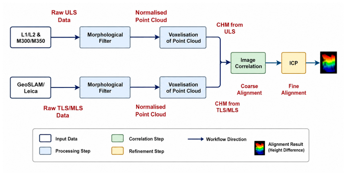
Figure 2.
Performance of voxel-based imputation when computing DBH for tall pine trees: (left) TreeLS on MLS data, (centre-left) regression model on ULSMLS data, (centre-right) regression model on ULSALL, and voxel-based imputation on ULSALL (right).
Figure 2.
Performance of voxel-based imputation when computing DBH for tall pine trees: (left) TreeLS on MLS data, (centre-left) regression model on ULSMLS data, (centre-right) regression model on ULSALL, and voxel-based imputation on ULSALL (right).
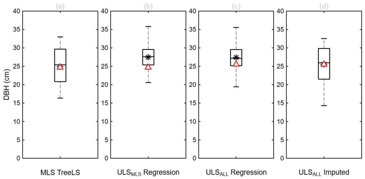
Figure 3.
Performance of voxel-based imputation in computing DBH for medium pine trees: (left) TreeLS on MLS data, (centre-left) regression model on ULSMLS data, (centre-right) regression model on ULSALL, and voxel-based imputation on ULSALL (right).
Figure 3.
Performance of voxel-based imputation in computing DBH for medium pine trees: (left) TreeLS on MLS data, (centre-left) regression model on ULSMLS data, (centre-right) regression model on ULSALL, and voxel-based imputation on ULSALL (right).
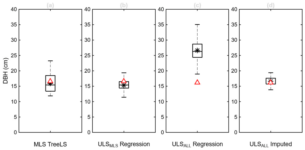
Figure 4.
Performance of voxel-based imputation in computing DBH for mature eucalyptus trees: (left) TreeLS on MLS data, (centre-left) regression model on ULSMLS data, (centre-right) regression model on ULSALL, and voxel-based imputation on ULSALL (right).
Figure 4.
Performance of voxel-based imputation in computing DBH for mature eucalyptus trees: (left) TreeLS on MLS data, (centre-left) regression model on ULSMLS data, (centre-right) regression model on ULSALL, and voxel-based imputation on ULSALL (right).
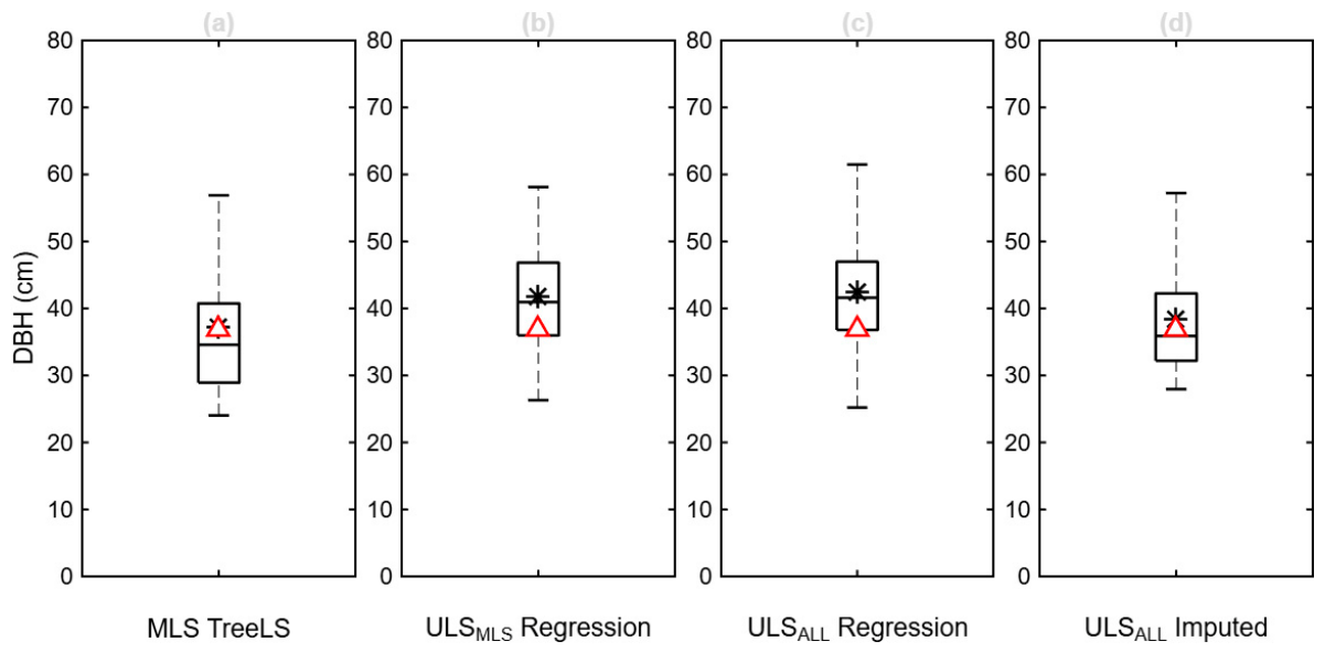

Table 1.
ULS Configuration for L1 and L2 LiDAR flights.
| L1 | L2 | |
|---|---|---|
| Flight speed | 3 m/s | 3 m/s |
| Returns | Triple (3) | Penta (5) |
| Sample rate | 160 Hz | 240 Hz |
| Mode | Repetitive Line Scan | Repetitive Line Scan |
| LiDAR flight strip overlap | 70 % | 70 % |
| Maximum Range | 450 m & 190 m (80% & 10% Reflectivity) |
450 m & 250 m (50% & 10% Reflectivity) |
| Manufacturer Accuracy | Horizontal: 10 cm @ 50 m Vertical: 5 cm @ 50 m |
Horizontal: 5 cm @ 150 m Vertical: 4 cm @ 150 m |
| Point Cloud Density | 2,100 points/m2 | 9,500 points/m2 |
Table 2.
TreeLS parameters used in tree segmentation and stem mapping.
| Parameter | Tall Radiata Pine | Medium Radiata Pine | Mature Eucalyptus |
| DBHWindow (m) | [1.15 1.55] | [1.20 1.45] | [1.10 1.70] |
| TargetDBHHeight (m) | 1.3 | 1.3 | 1.3 |
| CrownMinHeight (m) | 3 | 3 | 3 |
| MapVoxelSizes (m) | [0.05 0.075 0.10 0.15] | [0.10 0.15 0.20 0.25] | [0.10 0.15 0.20 0.25] |
| StemVoxelSize (m) | 0.015 | 0.03 | 0.03 |
| CircleTrimQuantile (m) | 0.6 | 0.28–0.35 | 0.65–0.75 |
| FitRadiusLimits (m) | [0.06 0.45] | [0.04 0.22] | [0.08 0.60] |
| RadiusRangeLoose (m) | [0.06 0.40] | [0.08 0.165] | [0.10 0.60] |
| RadiusRangeClean (m) | [0.08 0.35] | [0.09 0.145] | [0.12 0.50] |
| ErrorLooseBase (m) | 0.1 | 0.08 | 0.12–0.14 |
| ErrorLooseRadiusFactor (m) | 0.4 | 0.35 | 0.45–0.50 |
| ErrorCleanMax (m) | 0.08 | 0.05 | 0.10–0.12 |
| RelErrorSuspect (m) | 0.55 | 0.35 | 0.60–0.70 |
| ErrorSuspect (m) | 0.1 | 0.1 | 0.12–0.14 |
| LargeRadiusSuspect (m) | 0.35 | 0.2 | 0.45–0.50 |
| LargeRadiusErrorSuspect (m) | 0.1 | 0.06 | 0.12–0.14 |
| NLooseMin | 20 | 20 | 20 |
| NCleanMin | 30 | 40 | 30–35 |
| LowDensityN | 20 | 30 | 20–25 |
| CleanMinTrees | 50 | 200 | 30–50 |
| CleanMinFractionOfLoose | 0.25 | 0.35 | 0.20–0.25 |
Table 3.
Summary of mean values of all tree attributes extracted from point clouds using LDTIM and regression model vs field measurements for radiata pine site.
Table 3.
Summary of mean values of all tree attributes extracted from point clouds using LDTIM and regression model vs field measurements for radiata pine site.
| Attribute | ULS High Res | ULS Low Res | MLS | FLS | Field Measurements |
| All Tall Trees | |||||
| HT (m) | 20.8 ± 3.7 | 19.8 ± 3.0 | 19.8 ± 5.0 | 20.8 ± 3.8 | 20.5 ± 1.6 |
| CD (m) | 4.6 ± 0.4 | 4.7 ± 1.5 | 4.4 ± 0.9 | 4.5 ± 0.4 | 2.7 ± 0.6 |
| DBH (cm) | 27.4 ± 3.1 | 27.9 ± 0.4 | 27.5 ± 3.9 | 27.7 ± 3.0 | 25.5 ± 4.8 |
| All Medium Trees | |||||
| HT (m) | 11.2 ± 2.4 | 11.1 ± 2.5 | 11.0 ± 2.7 | 11.3 ± 1.9 | 11.4 ± 1.1 |
| CD (m) | 3.1 ± 0.4 | 3.1 ± 0.5 | 3.1 ± 0.8 | 3.1 ± 0.7 | 2.2 ± 0.4 |
| DBH (cm) | 26.6 ± 5.2 | 26.2 ± 5.3 | 15.3 ± 3.7 | 26.9 ± 2.9 | 16.4 ± 2.5 |
Table 4.
DBH means derived using TreeLS and regression models vs field measurements for the MLS and ULS-only pine tree sub-sets.
Table 4.
DBH means derived using TreeLS and regression models vs field measurements for the MLS and ULS-only pine tree sub-sets.
| Tree Set | TreeLS Model | Regression Model | Field Measurements | ||||
| ULS | MLS | FLS | ULS | MLS | FLS | ||
| MLS Trees, Tall | - | 24.9 | 24.4 | 27.4 | 27.5 | 27.2 | 24.7 ± 5.3 |
| ULS-only Trees Tall | - | - | - | 27.7 | - | - | 25.5 ± 2.7 |
| MLS Trees Medium | - | 15.9 | 17.7 | 26.6 | 12.5 | 26.9 | 16.6 ± 1.3 |
| ULS-only Trees Medium | - | - | - | 26.6 | - | - | 16.4 ± 3.1 |
Table 5.
Mean of field measurements for eucalyptus trees and attributes extracted using TreeLS. Due to time constraints tree height and crown diameter were not measured in the field, so no direct field-based validation of LiDAR-derived estimates was possible.
Table 5.
Mean of field measurements for eucalyptus trees and attributes extracted using TreeLS. Due to time constraints tree height and crown diameter were not measured in the field, so no direct field-based validation of LiDAR-derived estimates was possible.
| Attribute | L1 ULS | L2 ULS | MLS | L1 FLS | L2 FLS | Field Measurements |
| HT (m) | 32.1 ± 2.8 | 32.4 ± 3.0 | 30.9 ± 5.0 | 31.9 ± 3.8 | 32.2 ± 3.8 | -- |
| CD (m) | 6.5 ± 0.4 | 9.6 ± 1.5 | 5.9 ± 0.9 | 6.0 ± 0.4 | 10.2 ± 3.8 | -- |
| DBH (cm) | 34.4 ± 3.1 | 37.8 ± 0.4 | 37.5 ± 3.9 | 41.3 ± 3.0 | 42.0 ± 3.8 | 36.9 ± 8.8 |
Table 6.
Mean imputation estimates of DBH for tall and medium pine and mature eucalyptus plantations based on FLS training data. The values in parentheses are differences from the field measurements, which are for ULS_ALL regions. Values are coloured blue if they are low and red if they are high.
Table 6.
Mean imputation estimates of DBH for tall and medium pine and mature eucalyptus plantations based on FLS training data. The values in parentheses are differences from the field measurements, which are for ULS_ALL regions. Values are coloured blue if they are low and red if they are high.
| Observation or Imputation Strategy | Tree Set & DBH in cm (and Errors) | |||
|---|---|---|---|---|
| Radiata Pine | Eucalyptus | |||
| Tall | Medium | Tall | ||
| Field Observations (Target Value) | 25.4 ± 5.3 | 16.2 ± 1.3 | 36.9 ± 8.8 | |
| Strategy 1 | Direct Adjustment of Model | 26.9 (1.5) | 17.1 (0.9) | 27.4 (1.3) |
| Strategy 2 | Weighted Adjustment of Model | 29.1 (3.7) | 26.1 (9.9) | 37.8 (0.8) |
| Strategy 3 | Beta Function CDFs | 24.4 (1.0) | 17.4 (1.2) | 37.6 (0.7) |
| Strategy 4 | Weibull Function CDFs | 24.5 (0.9) | 17.9 (1.7) | 37.4 (0.5) |
| Strategy 5 | Nakagami Function CDFs | 24.4 (1.0) | 17.8 (1.6) | 37.4 (0.5) |
| Strategy 6 | Normal Function CDFs | 24.4 (1.0) | 17.8 (1.6) | 37.8 (0.9) |
| Strategy 7 | Log-Normal Function CDFs | 24.4 (1.0) | 17.8 (1.6) | 37.5 (0.6) |
| Strategy 8 | Empirical Quantile Imputation | 24.4 (1.0) | 17.8 (1.6) | 37.6 (0.7) |
| Strategy 9 | Rank-Based Quantile Imputation | 24.4 (1.0) | 17.8 (1.6) | 37.8 (0.9) |
| Strategy 10 | Conditional Mean/Spread Restoration | 24.4 (1.0) | 17.8 (1.6) | 37.8 (0.9) |
| Strategy 11 | Voxel-Based Imputation | 24.6 (0.8) | 17.6 (1.4) | 39.2 (2.2) |
| Regression Model (No Imputation) | 27.4 (2.0) | 26.6 (10.4) | 42.3 (5.4) | |
Table 7.
Mean imputation estimates of DBH for tall and medium pine and mature eucalyptus plantations based on MLS training data. The values in parentheses are differences from the field measurements, which are for ULS_ALL regions. Values are coloured blue if they are low and red if they are high.
Table 7.
Mean imputation estimates of DBH for tall and medium pine and mature eucalyptus plantations based on MLS training data. The values in parentheses are differences from the field measurements, which are for ULS_ALL regions. Values are coloured blue if they are low and red if they are high.
| Observation or Imputation Strategy | Tree Set & DBH in cm (and Errors) | |||
|---|---|---|---|---|
| Radiata Pine | Eucalyptus | |||
| Tall | Medium | Tall | ||
| Field Observations (Target Value) | 25.4 ± 5.3 | 16.2 ± 1.3 | 36.9 ± 8.8 | |
| Strategy 1 | Direct Adjustment of Model | 25.8 (0.4) | 13.7 (2.5) | 38.2 (1.3) |
| Strategy 2 | Weighted Adjustment of Model | 28.6 (3.2) | 25.5 (1.4) | 43.4 (6.5) |
| Strategy 3 | Beta Function CDFs | 24.8 (0.6) | 16.5 (0.3) | 37.4 (0.5) |
| Strategy 4 | Weibull Function CDFs | 25.1 (0.3) | 16.0 (0.2) | 37.0 (0.1) |
| Strategy 5 | Nakagami Function CDFs | 24.9 (0.3) | 16.0 (0.2) | 37.4 (0.5) |
| Strategy 6 | Normal Function CDFs | 24.9 (0.3) | 16.0 (0.2) | 37.3 (0.4) |
| Strategy 7 | Log-Normal Function CDFs | 24.9 (0.3) | 16.0 (0.2) | 37.4 (0.5) |
| Strategy 8 | Empirical Quantile Imputation | 24.9 (0.3) | 15.9 (0.3) | 37.4 (0.5) |
| Strategy 9 | Rank-Based Quantile Imputation | 24.9 (0.3) | 15.9 (0.3) | 37.5 (0.6) |
| Strategy 10 | Conditional Mean/Spread Restoration | 24.9 (0.3) | 15.9 (0.3) | 37.5 (0.6) |
| Strategy 11 | Voxel-Based Imputation | 25.5 (0.1) | 16.5 (0.3) | 37.7 (0.8) |
| Regression Model (No Imputation) | 27.4 (2.0) | 26.6 (10.4) | 42.3 (5.4) | |
Disclaimer/Publisher’s Note: The statements, opinions and data contained in all publications are solely those of the individual author(s) and contributor(s) and not of MDPI and/or the editor(s). MDPI and/or the editor(s) disclaim responsibility for any injury to people or property resulting from any ideas, methods, instructions or products referred to in the content. |
© 2026 by the authors. Licensee MDPI, Basel, Switzerland. This article is an open access article distributed under the terms and conditions of the Creative Commons Attribution (CC BY) license (http://creativecommons.org/licenses/by/4.0/).
Copyright: This open access article is published under a Creative Commons CC BY 4.0 license, which permit the free download, distribution, and reuse, provided that the author and preprint are cited in any reuse.


