
Submitted:
05 July 2026
Posted:
06 July 2026
You are already at the latest version
Abstract
The vibration response of a cracked ice shelf to tsunami wave forcing is studied. In particular, the tsunami induced calving events in the Sulzberger Ice Shelf in 2011 and 2022, is investigated. The time-domain response is reconstructed from the wave-frequency response, and the stress field is calculated to evaluate the crack-tip stress intensity. Assuming that crack growth is governed by the Paris Law, the fatigue growth constant for this ice shelf is estimated. This work is presented as a preliminary study demonstrating how these rare geophysical phenomena can be used to estimate critical material parameters.
Keywords:
tsunami wave
; ice shelf
; cracked ice shelf
; stress
; Paris' law
1. Introduction
Ice shelves are floating extensions of land-based glaciers and play a pivotal role in modulating ice discharge into the ocean. Their structural integrity is threatened by the formation and propagation of cracks, which can lead to large-scale calving events and contribute to rising sea level [1,2]. Understanding the vibration response of cracked ice shelves to ocean wave forcing is therefore essential to predict their mechanical behaviour and failure modes. Beginning with the work of [3], it has been suggested that the impact of the repetitive flux of ocean waves on the ice shelf could cause the calving of glacier tongues. This hypothesis has received significant evidence in recent years [4,5]. In [4], they show evidence that seasonal loss of sea ice reduces the natural buffer, allowing ocean swells to flex the vulnerable outer ice-shelf margins and weaken them to the point of calving. This scenario is especially troubling given the decline in Antarctic sea ice [6,7,8].
In this study, we focus on two tsunami triggers of ice shelf calving: the Honshu earthquake and the Hunga-Tonga volcanic eruption. As reported in [9], the Honshu earthquake triggered a tsunami that resulted in the calving of the Sulzberger ice shelf , east of the Ross ice shelf) on 11 March 2011. As a result of this event, two icebergs formed near Antarctica. On the other hand, On January 15, 2022, around 4:15 a.m., the Hunga Tonga Volcano in the Islands of Tonga in the southwest Pacific Ocean triggered a tsunami in the Pacific Ocean. As a result, the West Sulzberger Ice Shelf (WSIS) experienced a significant calving event after the tsunami event. The calving occurred between January 15 and January 18, 2022 [10,11]. In this event, the WSIS lost approximately 106 of ice, reducing its size to the smallest recorded since 1948 [12]. We chose these events because we can reconstruct to some accuracy the wave forcing and subsequent strain induced on the ice shelf. This, in turn, allows us to estimate the parameters that may control the crack growth in ice shelves. In particular, the evidence from the tsunami induced calving seems to suggest that the slow ringing of the tsunami wave induced crack growth through cyclic loading, implying that this process maybe governed by a Paris type law.
In this paper and building on previous studies of floating elastic beams [13,14,15,16], we model the cracked ice shelf as a thin beam of constant thickness floating in shallow water [17], where the crack is represented as a rotational spring whose stiffness depends on the depth ratio of the crack, following the formulation [16,18,19,20]. The cracked ice shelf domain is divided into three regions, and analytical solutions are constructed in each region using modal decomposition. Continuity conditions at the interfaces and a rotational compatibility condition at the crack yield a system of ten equations for the modal amplitudes. Later, we investigate the dynamic response of a cracked ice shelf subjected to tsunami wave-induced vibrations, with a particular focus on modelling crack growth using Paris’ Law [21,22]. For ice, the first attempt to apply the Paris law was reported in [23], where the authors presented preliminary results on fatigue crack growth on freshwater ice. They found evidence of crack growth that occurred under cyclic loading, although the data was insufficient to determine the validity of the behaviour of and . Later, in [24], they present preliminary results from fatigue tests in Antarctica. In contrast, several studies in engineering have used Paris’ law to determine the growth of fatigue cracks in various materials [25,26,27]. In [28], they established a procedure for analysing the crack propagation in a ship by using the Paris’ law in combination with the Monte Carlo technique. Also in [29], they study the effect of low temperature on fatigue crack propagation rates in a polar ship using the Paris law in their fatigue crack propagation test. Moreover, we provide a time domain solution and calculate the stress, which we used to compute the stress intensity factor, and fatigue crack growth in modelling Paris’ Law [30]. This approach provides a physics-based framework for simulating progressive fracture in ice shelves and assessing the impact of a tsunami wave on their stability.
The outline of the paper is as follows. In section 2 we investigate in detail the tsunami wave forces as measured near the Sulzberger ice shelf. We show that the waves for both tsunamis were similar. In section 3 we present our simple model for a cracked ice shelf and investigate the response of the ice shelf to the measured tsunami waves in the time domain in section 4. In section 5 we consider the application of Paris law and we give an estimate of the Paris law coefficient which controls the fatigue crack growth rate for an ice shelf, on the assumption the Paris growth law is appropriate.
2. Observational Tsunami Data
We present here measurements of the tsunami wave forcing made by tide gauges. We note that it was not possible to obtain the measurements exact on the Sulzberger ice shelf. For the Honshu Earthquake, the tsunami record used in this study was obtained from the ROBT tide-gauge station (10–20 March 2011) (see Figure 1 (a) ). For the Hunga-Tonga volcanic eruption, we use two tide gauge station datasets showing sea level changes during the volcanic event: the Antarctica Base station , located on the northwest of the Antarctic Peninsula, and the Cape Robert station , situated near the Ross Ice Shelf [12]. The tsunami wave amplitude for both stations is shown in Figure 1 (b) from 15 to 20 January 2022. We note that the iceberg experiences the tsunami waves as a slowly decaying wave which last for one to two hundred hours. Both tsunami waves are remarkably similar. We note the amplitude is around 10 cm in both cases.
2.1. Methods and Results
Building on the previous observations, we applied a high-pass filter on the tide-gauge record with a cutoff period of 2 hours to smooth the wave amplitude, remove low-frequency tidal and background ocean motion, and isolate the tsunami signal (see Figure 2).
The filtered record was then transformed into the frequency domain using a Fast Fourier Transform (FFT) to convert the signal in the time-domain to its representation in the frequency domain, as in Figure 3 and Figure 4.
The tsunami spectrum exhibits several distinct energy peaks rather than a single dominant frequency. Therefore, to represent the tsunami forcing in our model, a multi-peak Gaussian fitting approach was applied to the filtered tidal-gauge spectrum. Each of the Gaussian functions was given by
These individual Gaussian components were then superimposed to form a composite spectrum that closely follows the shape and amplitude of the measured tsunami frequency content. Figure 4 shows the fitted Gaussian function for the tsunami amplitude for each tide gauge in both tsunami cases.
This method enables us to use a synthetic spectrum to simulate the broadband characteristics of the real tsunami signal, rather than representing it as a mono-frequency wave.
In our model, we are dealing with a long-wave tsunami and can model the ice shelf as floating on shallow water leading to the following dispersion relation:
where is the angular frequency, g is the acceleration of gravity, and H is the depth of the water. Therefore, the wavenumber is equal to
Now, transforming from the frequency domain to the wavenumber domain, the Gaussian in wavenumber is:
To examine the distribution of tsunami energy across multiple frequency decades, we used Log-log spectral plots. As before, we fitted multiple Gaussian functions to approximate the tsunami frequency spectrum. In logarithmic scaling, the visibility of both dominant low-frequency components and weaker higher-frequency oscillations becomes clearer. In Figure 5, the majority of the tsunami energy is concentrated within the Hz band, confirming the long-period nature of the tsunami forcing relevant to ice-shelf vibration.
In Figure 6, we made a compression between the tide-gauge record with the high-pass filter and the inverse Fourier transform of the fitted spectra, to see the precision of the fitted Gaussian tsunami spectrum.
We conclude from our analysis of these wave data for the tsunamis that the forcing in both cases was roughly similar with an amplitude of around 10 cm and with distinct spectral peaks. We note that the origin of these spectral peaks is not clear. We will consider the stress at the crack due to each of these frequencies in turn. To keep the analysis simple we set the peak response to 10 cm.
3. Vibration of a Cracked Ice Shelf Due to Transient Wave Forcing
Our model aims to simulate the motion of a cracked ice shelf to tsunami wave forcing. We begin by simulating the effect of a crack. The methodological analysis to simulate a cracked ice shelf is based on [13] and [16]. For completeness we give the theory here.
To determine the flexure of an ice shelf with a through-thickness crack, we model the shelf as a thin elastic beam floating on the ocean. The crack is assumed to be located at a fixed position , and it modifies the boundary conditions of the system (see Figure 7). The displacement of the ice shelf is denoted , and the wave forcing is described by the velocity potential .
The governing thin-beam approximation leads to
where is the flexural rigidity of the shelf. Here, GPa is the effective Young’s modulus, is Poisson’s ratio, is the ice density, is the water density, and is gravitational acceleration.
By assumption, the water potential and the vertical displacement u are coupled through the shallow-water equation [17]:
where H is the (constant) water depth [31]. Figure 7 provides a schematic diagram of the cracked ice shelf.
To proceed, we follow [13] and assume harmonic time dependence. That is, we write.
where is the angular frequency. This frequency-domain representation is not simply a “simplification,” but a standard Fourier-based approach: it enables us to solve for monochromatic wave responses, from which more general wave packets can be reconstructed by superposition. Substituting these forms yields
and
From these two coupled equations, we derive a sixth-order equation for :
The open-water limit (no ice above) reduces to
To solve the differential equation for the whole domain, we divide the system into three regions with different properties: (i) the region landward of the crack, (ii) the region seaward of the crack, and (iii) the open water. The governing equations in each region can be summarized as
where L denotes the crack position.
This framework can then be extended to more complicated configurations, such as multiple cracks or spatially varying elastic properties. Here, for clarity, We assume constant ice thickness, Young’s modulus, and density. Thus, the solution can be written as
In the open water, the wave-numbers are
and the roots and can be found by the following equations
Here, too, the roots come in pairs. As we mentioned in the previous case, we will choose the roots with positive sign only for both real and imaginary parts for the roots and . However, if a root is a complex number, we choose the positive real part.
In the case of the cracked ice shelf, the system is governed by ten boundary and continuity conditions. Four of these are imposed at the free edge (), and are expressed as follows:
The remaining six conditions are associated with the crack and the edge at , consisting of two continuity conditions at the plate end and four at the cracked section, as described in [19]:
To account for the influence of the crack on the ice shelf’s slope continuity, an additional compatibility condition is introduced:
where represents the rotational spring stiffness modelling the crack. Here, h denotes the ice thickness, and is a compliance function dependent on the crack depth ratio, given by:
as reported in [16,19,20,32].
These ten conditions yield a system of linear equations of the form , where is the coefficient matrix representing the boundary conditions, and is the vector of unknown coefficients.
Moreover, the equations for the displacement u are
Here . Figure 8 shows the displacement u for the cracked ice.
4. Time-Domain Solutions
To simulate the motion in the time domain, we will use the given formula
where is the wave number in the left-hand incident region, and
We take to be 10 cm.
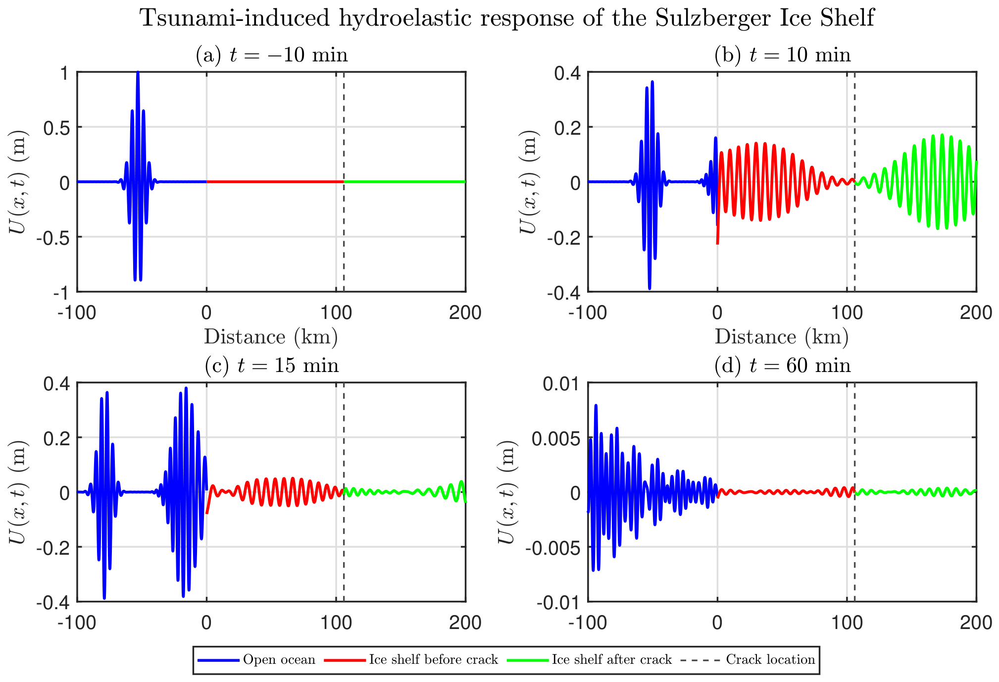
After the simulations, we found that long-period tsunami waves were smoothly transmitted through the Sulzberger Ice Shelf without reflection or noticeable bending at the crack (see Figure 9 and Figure 10). The reason is that the tsunami has low-frequency forcing around up to and wavelengths that are extremely large relative to the characteristic dimensions of the ice shelf and the geometry of the crack. Consequently, the incident wave energy is transmitted efficiently through the ice shelf. To further investigate the influence of wave frequency on hydroelastic behaviour, additional simulations were performed using progressively higher forcing frequencies, up to (see Figure 11). Increasing the forcing frequency reduces the wavelength of the incident wave, enhancing its interaction with the ice-shelf geometry and crack discontinuity. Under these higher-frequency conditions, the reflection becomes visible, with wave energy reflecting toward the open ocean after interacting with the ice shelf.
These results indicate that tsunami-frequency waves primarily behave as long, shallow-water waves that propagate through the ice shelf with minimal reflection. In contrast, shorter-wavelength forcing produces stronger hydroelastic interactions, localised oscillations, and increased reflected wave energy.
4.1. The Crack Stress in the Time Domain
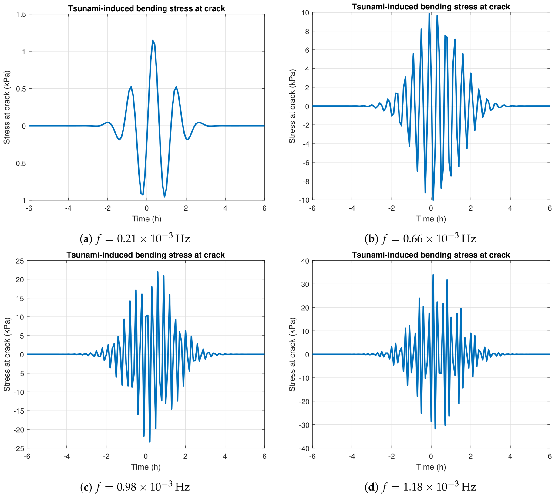
The bending stress at the crack location in the ice shelf is obtained from the second spatial derivative of the displacement field. The expression is given by:
where is the distance from the neutral axis to the upper or lower ice surface, and is the second derivative of the displacement with respect to x at the location of the crack.
We start by taking the second derivative of in the frequency domain. The governing expressions for are derived from the modal decomposition solution and are given by:
where are modal coefficients determined from boundary and continuity conditions, and are characteristic roots of the system, and R is the reflection coefficient.
The stress range is then defined by:
Figure 12.
Stress distributions along the ice shelf corresponding to four dominant tsunami frequencies.
Figure 12.
Stress distributions along the ice shelf corresponding to four dominant tsunami frequencies.
5. Paris’ Law and Crack Growth Phases in Ice Shelves
Predicting crack growth in ice shelves is essential for understanding their stability and the potential impacts on global sea levels. Here, we have used Paris’ law to estimate the fatigue crack growth induced by the tsunami wave and estimate the number of cycles until the ice shelf eventually breaks [33]. The law is given by
where C and m are material fatigue parameters , N is the number of loading cycles, a is the crack depth, and is the stress intensity factor range, given by:
where h is the ice thickness, is the tsunami-induced stress range, and is a dimensionless geometry correction factor that accounts for the finite thickness of the ice shelf and the relative crack depth. In this study, the crack was treated as a single-edge crack propagating through the ice thickness, so the correction factor was expressed as a function of the crack-depth ratio [18,21], therefore
Critical to our work is trying to obtain an estimate of C, which is highly dependent on the material in question.

Table 1.
Paris’ law results for the analyzed tsunami frequencies in the Figure 4(a):
Table 1.
Paris’ law results for the analyzed tsunami frequencies in the Figure 4(a):
| f (Hz) | (MPa) | (MPa) |
|---|---|---|
| 2.1007e-04 | 2.1432e-02 | |
| 4.8134e-04 | 4.9110e-02 | |
| 1.1818e-03 | 1.2058e-01 | |
| 1.9883e-03 | 2.0286e-01 | |
| 3.0268e-03 | 3.0883e-01 | |
| 4.5362e-03 | 4.6289e-01 | |
| 5.7200e-03 | 5.8378e-01 | |
| 6.5545e-03 | 6.6905e-01 |
There is no clear evidence of Paris’ law constants for a large-scale ice shelf in any previous studies. For m we adopted a value that is commonly used in fatigue growth, which is . For the coefficient C we estimate it using the observed calving timescale of the Sulzberger Ice Shelf following the 2011 and 2022 tsunamis which in both cases was around 3 days.
Our estimate is based on the observation that there was significant energy up to around , corresponding to a period of . Since the calving event occurred approximately three days after the tsunami [9], the corresponding number of loading cycles is 306. By assuming that the crack propagates from the initial crack depth to the critical crack depth the required average crack growth per cycle is . This gives a value of As a final remark, we want to make clear that we cannot be sure that Paris law applies to crack growth in ice shelves, and if it does, this can only be seen as giving an order of magnitude estimate.
6. Discussion
We have shown that the tsunami wave forcing, which induced calving events in the Sulzberger ice shelf in 2011 and 2022, was of similar magnitude and spectral range. We simulate this ice shelf with these wave forces and a crack using a simple one dimensional model. We used our results to estimate the value of the critical fatigue growth parameter, C, in the Paris law. We see this as a preliminary study showing how these rare geophysical phenomena can be used to give estimates of critical parameters. The next step is to consider the effect of ocean wave swell on crack growth using our estimated value of C and more sophisticated crack growth and ice shelf models.
Author Contributions
Conceptualization, A.A. and M.M.; methodology, A.A.; software, A.A.; validation, A.A., writing—original draft preparation, A.A.; writing—review and editing, M.M.; visualization, A.A; supervision, M.M. All authors have read and agreed to the published version of the manuscript.
Funding
The authors extend their appreciation to the Deanship of Scientific Research at Northern Border University, Arar, KSA for funding this research work through the project number “NBUSAFIR- 2026 which supported A.A.
Data Availability Statement
Data is available from the authors on request.
Conflicts of Interest
The authors declare no conflicts of interest.
References
- Scambos, T.A.; Bohlander, J.; Raup, B. Ice shelf evolution and collapse. The Cryosphere 2017, 11, 1511–1524.
- Bassis, J.N.; Jacobs, S. Diverse calving patterns linked to glacier geometry. Nature Geoscience 2013, 6, 833–836. [CrossRef]
- Holdsworth, G.; Glynn, J. Iceberg calving from floating glaciers by a vibrating mechanism. Nature 1978, 274, 464–466. [CrossRef]
- Massom, R.A.; Scambos, T.A.; Bennetts, L.G.; Reid, P.; Squire, V.A.; Stammerjohn, S.E. Antarctic ice shelf disintegration triggered by sea ice loss and ocean swell. Nature 2018, 558, 383–389. [CrossRef]
- Bennetts, L.G.; Liang, J. Modelling dynamic strains on ice shelves resulting from flexural and extensional motions forced by ocean wave packets. The ANZIAM Journal 2026, 68, e4. [CrossRef]
- Li, X.; Cai, W.; Meehl, G.A.; Chen, D.; Yuan, X.; Raphael, M.; Holland, D.M.; Ding, Q.; Fogt, R.L.; Markle, B.R.; et al. Tropical teleconnection impacts on Antarctic climate changes. Nature Reviews Earth & Environment 2021, 2, 680–698. [CrossRef]
- Hanna, E.; Topál, D.; Box, J.E.; Buzzard, S.; Christie, F.D.; Hvidberg, C.; Morlighem, M.; De Santis, L.; Silvano, A.; Colleoni, F.; et al. Short-and long-term variability of the Antarctic and Greenland ice sheets. Nature Reviews Earth & Environment 2024, 5, 193–210. [CrossRef]
- Josey, S.A.; Meijers, A.J.; Blaker, A.T.; Grist, J.P.; Mecking, J.; Ayres, H.C. Record-low Antarctic sea ice in 2023 increased ocean heat loss and storms. Nature 2024, 636, 635–639. [CrossRef]
- Brunt, K.M.; Okal, E.A.; MacAyeal, D.R. Antarctic ice-shelf calving triggered by the Honshu (Japan) earthquake and tsunami, March 2011. Journal of Glaciology 2011, 57, 785–788. [CrossRef]
- Carvajal, M.; Sepúlveda, I.; Gubler, A.; Garreaud, R. Worldwide signature of the 2022 Tonga volcanic tsunami. Geophysical Research Letters 2022, 49, e2022GL098153. [CrossRef]
- Yamada, M.; Ho, T.C.; Mori, J.; Nishikawa, Y.; Yamamoto, M.Y. Tsunami triggered by the Lamb wave from the 2022 Tonga volcanic eruption and transition in the offshore Japan region. Geophysical Research Letters 2022, 49, e2022GL098752. [CrossRef]
- Zhao, A.; Cheng, Y.; Fraser, A.D.; Bennetts, L.G.; Xiao, H.; Liang, Q.; Li, T.; Li, R. Long-term evolution of the Sulzberger Ice Shelf, West Antarctica: Insights from 74-year observations and 2022 Hunga-Tonga volcanic tsunami-induced calving. Earth and Planetary Science Letters 2024, 646, 118958. [CrossRef]
- McNeil, S.; Meylan, M.H. Time-Dependent Modelling of the Wave-Induced Vibration of Ice Shelves. Journal of Marine Science and Engineering 2023, 11, 1191. [CrossRef]
- Meylan, M.H.; Bennetts, L.G.; Hosking, R.J.; Catt, E. On the calculation of normal modes of a coupled ice-shelf/sub-ice-shelf cavity system. Journal of Glaciology 2017, 63, 751–754. [CrossRef]
- Aljabri, R.; Meylan, M.H. Time Domain Vibration Analysis of an Ice Shelf. Journal of Marine Science and Engineering 2024, 12, 468. [CrossRef]
- Alshammari, A.; Meylan, M.H. Time Domain Vibration Analysis of Cracked Ice Shelf. Glacies 2025, 2, 5. [CrossRef]
- Stoker, J.J. Water waves: The mathematical theory with applications; Vol. 36, John Wiley & Sons, 1992.
- Wang, S.; Qiao, P.; Shivakumar, K. A continuous cracked beam vibration theory. Journal of Sound and Vibration 2006, 294, 23–46. [CrossRef]
- Mungla, M.J.; Sharma, D.; Makwana, H.; Bhavsar, R. Inverse dynamics of cracked cantilever beam. In Proceedings of the International Conference in Advanced Design and Manufacturing, 2014, pp. 331–336.
- Mungla, M.J.; Sharma, D.S.; Trivedi, R.R. Identification of a crack in clamped-clamped beam using frequency-based method and genetic algorithm. Procedia Engineering 2016, 144, 1426–1434. [CrossRef]
- Tada, H.; Paris, P.C.; Irwin, G.R. The stress analysis of cracks. Handbook, Del Research Corporation 1973, 34.
- Rist, M.A.; Sammonds, P.R.; Oerter, H.; Doake, C.S.M. Fracture of antarctic shelf ice. Journal of Geophysical Research: Solid Earth 2002, 107, ECV 3–1–ECV 3–13. [CrossRef]
- Nixon, W.A.; Weber, L.J. Fatigue-crack growth in fresh-water ice: preliminary results. Annals of glaciology 1991, 15, 236–241. [CrossRef]
- Haskell, T.; Robinson, W.; Langhorne, P. Preliminary results from fatigue tests on in situ sea ice beams. Cold regions science and technology 1996, 24, 167–176. [CrossRef]
- Pugno, N.; Ciavarella, M.; Cornetti, P.; Carpinteri, A. A generalized Paris’ law for fatigue crack growth. Journal of the Mechanics and Physics of Solids 2006, 54, 1333–1349. [CrossRef]
- Rajabipour, A.; Melchers, R.E. Application of Paris’ law for estimation of hydrogen-assisted fatigue crack growth. International Journal of Fatigue 2015, 80, 357–363. [CrossRef]
- Bazant, Z.P.; Hubler, M.H. Theory of cyclic creep of concrete based on Paris law for fatigue growth of subcritical microcracks. Journal of the Mechanics and Physics of Solids 2014, 63, 187–200. [CrossRef]
- Zhao, W.; Leira, B.J.; Feng, G.; Gao, C.; Cui, T. A reliability approach to fatigue crack propagation analysis of ship structures in polar regions. Marine Structures 2021, 80, 103075. [CrossRef]
- Zhao, W.; Feng, G.; Zhang, M.; Ren, H.; Sinsabvarodom, C. Effect of low temperature on fatigue crack propagation rates of DH36 steel and its butt weld. Ocean Engineering 2020, 196, 106803. [CrossRef]
- van der Veen, C.J. Fracture mechanics approach to glacier calving. Cold Regions Science and Technology 1998, 27, 31–47. [CrossRef]
- Meylan, M.H.; Bennetts, L.G.; Hosking, R.J.; Catt, E. On the calculation of normal modes of a coupled ice-shelf/sub-ice-shelf cavity system. Journal of Glaciology 2017, 63, 751–754. [CrossRef]
- Rizos, P.; Aspragathos, N.; Dimarogonas, A. Identification of crack location and magnitude in a cantilever beam from the vibration modes. Journal of sound and vibration 1990, 138, 381–388. [CrossRef]
- Paris, P.; Erdogan, F. A critical analysis of crack propagation laws. Journal of Basic engineering 1963, 85, 528–533. [CrossRef]
Figure 1.
(a)The tide gauge data for the Honshu Earthquake from March 10, 2011, to March 20, 2011. The data was obtained from https://sealevel-data.linz.govt.nz/index.html?tidegauge=ROBT; (b)The tide gauge data for Hunga-Tonga volcanic from January 15, 2022, to January 20, 2022 at the Antarctica Base station and the Cape Robert station. The data were obtained from https://webcritech.jrc.ec.europa.eu/SeaLevelsDb/Device/2478, and https://www.linz.govt.nz/products-services/data/types-linz-data/sea-level-data/sea-level-data-downloads/using-tsunami-tide-guage-data.
Figure 1.
(a)The tide gauge data for the Honshu Earthquake from March 10, 2011, to March 20, 2011. The data was obtained from https://sealevel-data.linz.govt.nz/index.html?tidegauge=ROBT; (b)The tide gauge data for Hunga-Tonga volcanic from January 15, 2022, to January 20, 2022 at the Antarctica Base station and the Cape Robert station. The data were obtained from https://webcritech.jrc.ec.europa.eu/SeaLevelsDb/Device/2478, and https://www.linz.govt.nz/products-services/data/types-linz-data/sea-level-data/sea-level-data-downloads/using-tsunami-tide-guage-data.
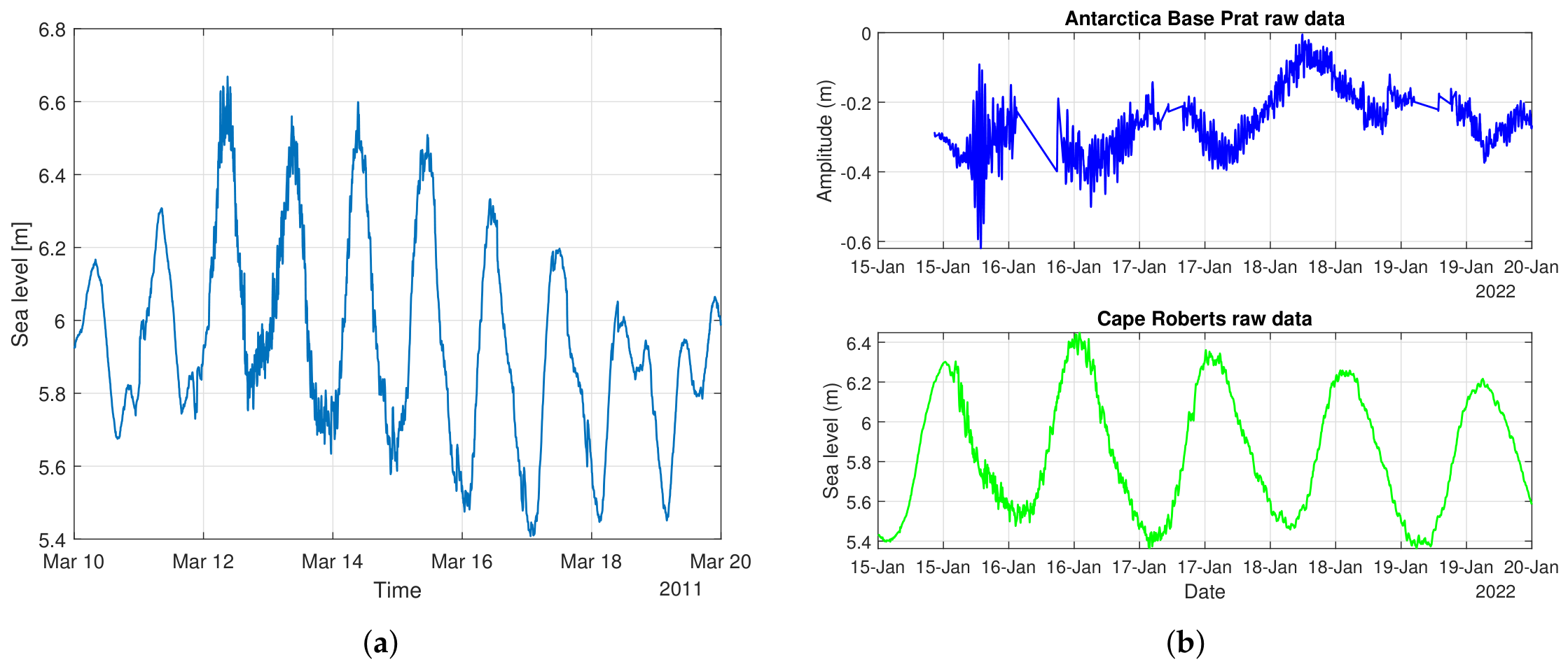
Figure 2.
sea-level record after applying a 2-h high-pass filter to isolate the tsunami band.
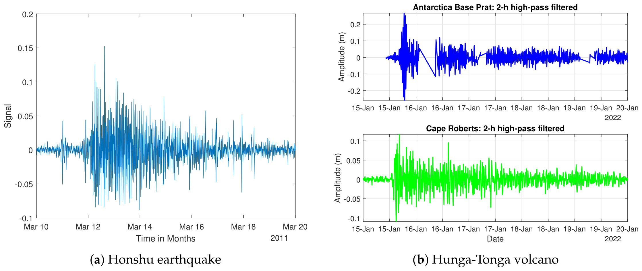
Figure 3.
The tsunami frequency spectrum.
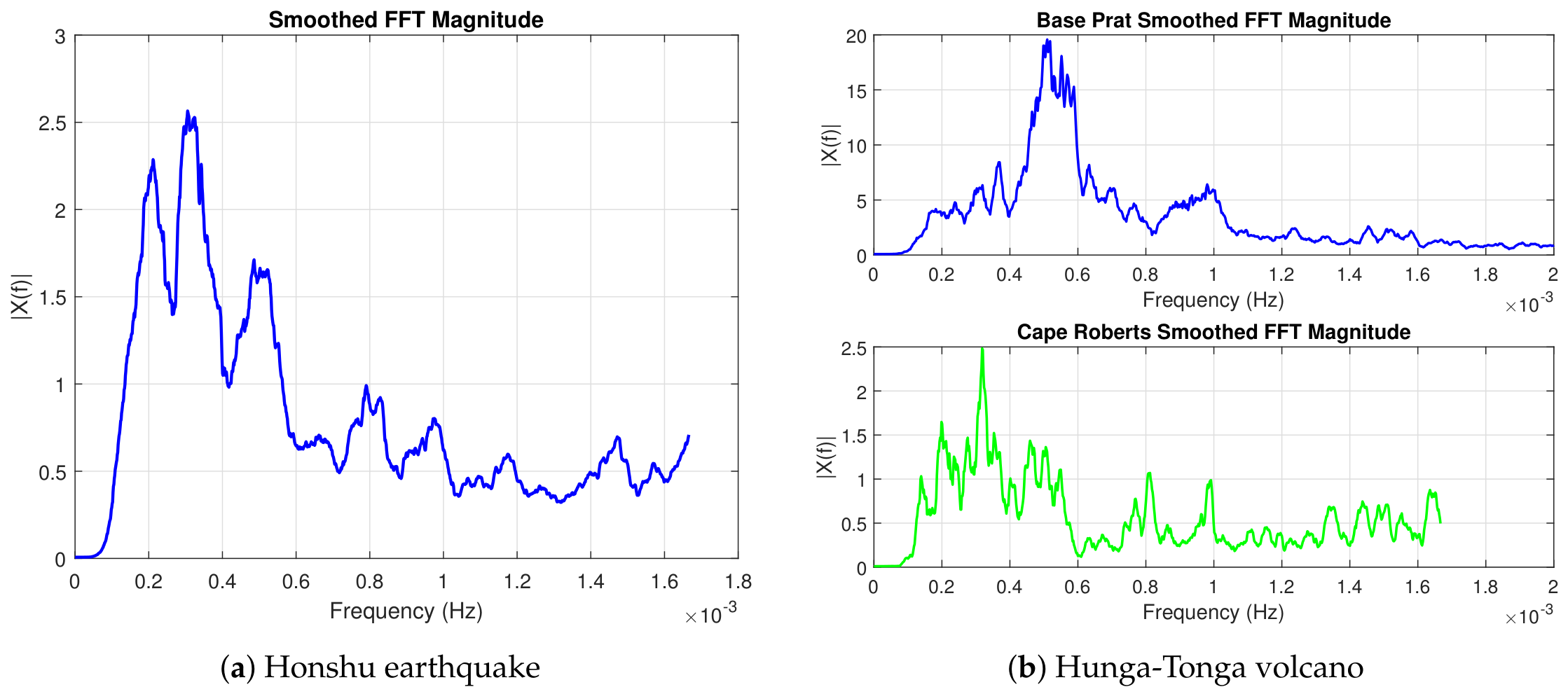
Figure 4.
Individual Gaussian functions fitted to the main energy peaks of the tsunami frequency spectrum. Each curve represents a single Gaussian centered at a dominant frequency observed in the high-pass filtered sea-level record.
Figure 4.
Individual Gaussian functions fitted to the main energy peaks of the tsunami frequency spectrum. Each curve represents a single Gaussian centered at a dominant frequency observed in the high-pass filtered sea-level record.
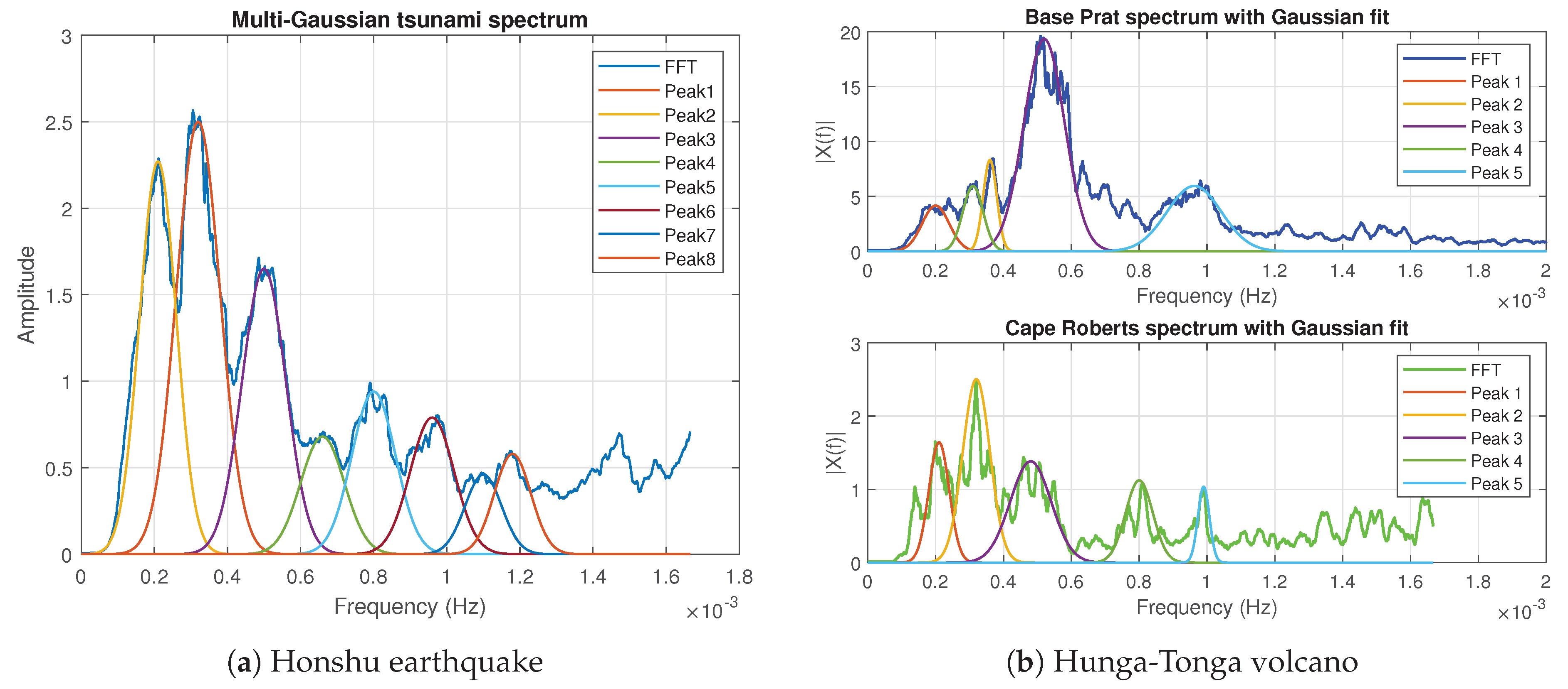
Figure 5.
log-log plot of the fitted Gaussian functions that approximate the tsunami frequency spectrum.
Figure 5.
log-log plot of the fitted Gaussian functions that approximate the tsunami frequency spectrum.
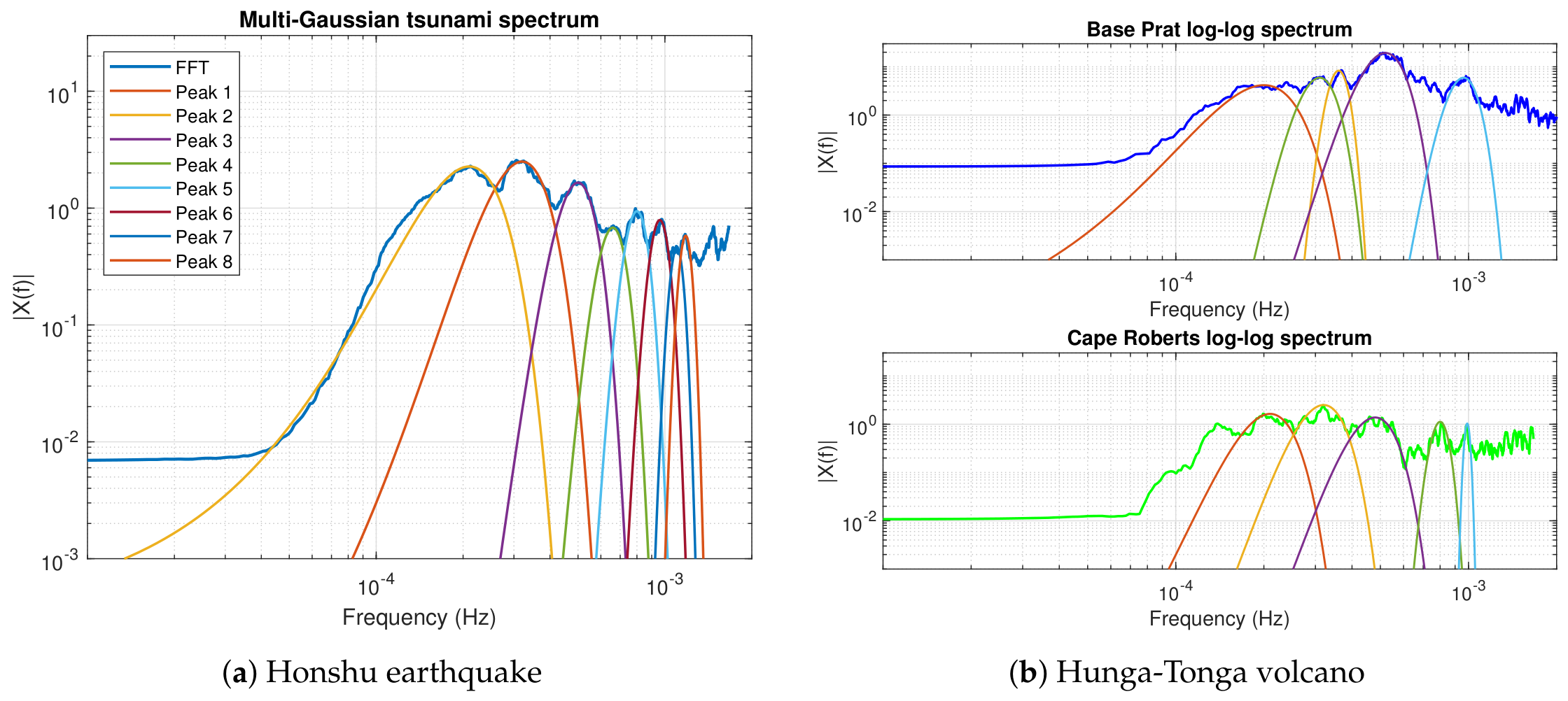
Figure 6.
A comparison plot between the tide-gauge record with the high-pass filter and the inverse Fourier transform.
Figure 6.
A comparison plot between the tide-gauge record with the high-pass filter and the inverse Fourier transform.
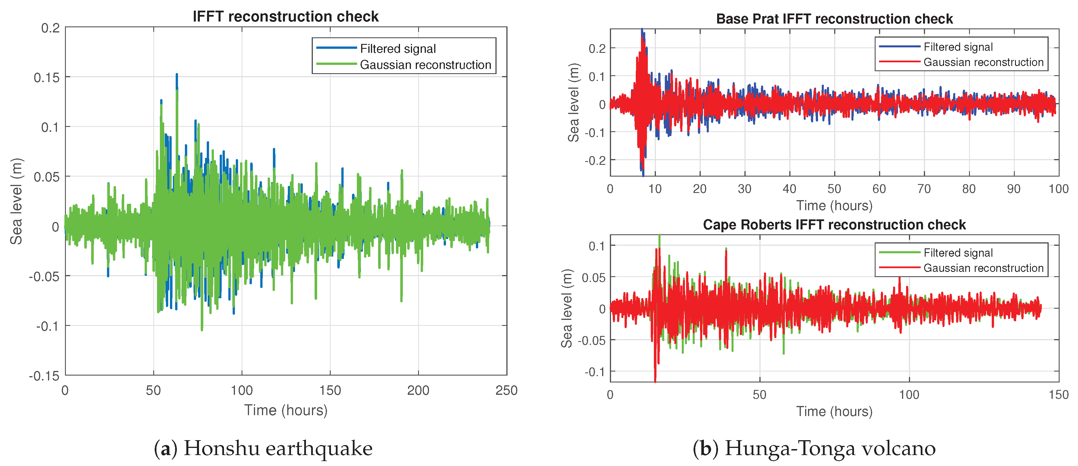
Figure 7.
Schematic diagram of a Cracked Ice Shelf.
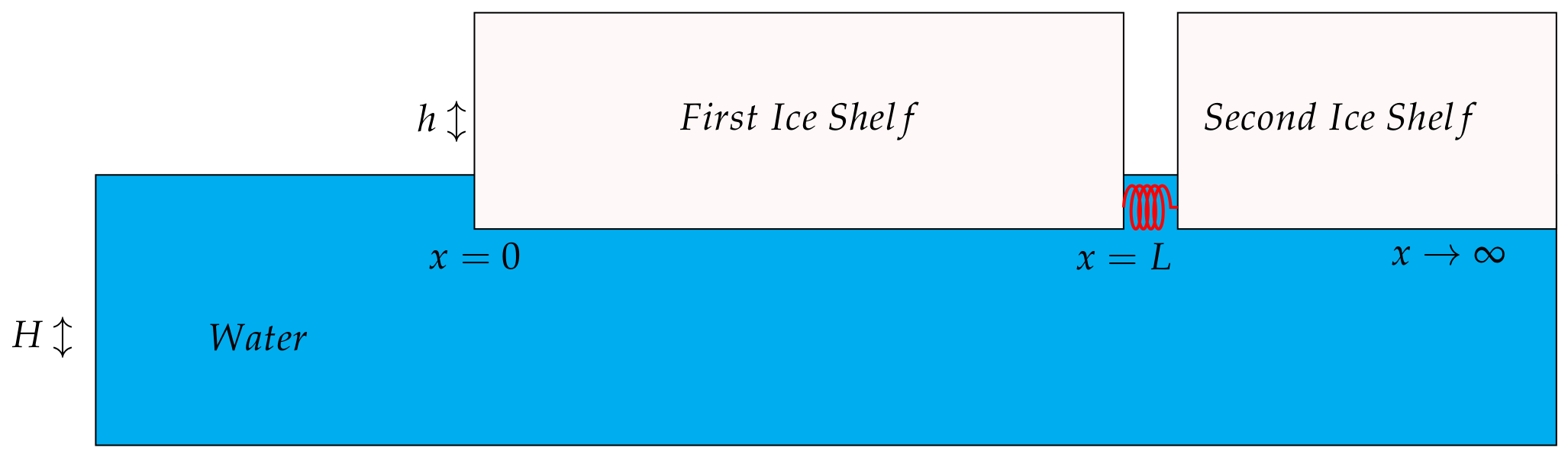
Figure 8.
plot for the ice shelf displacement.
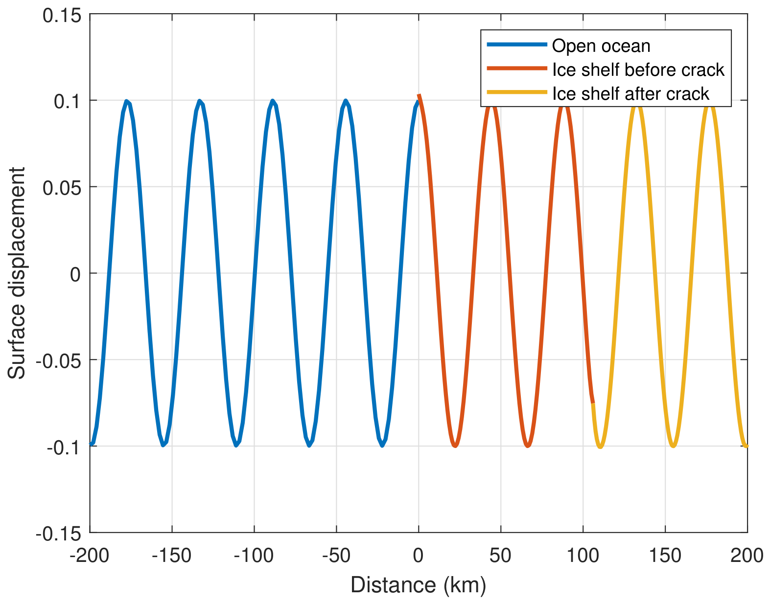
Figure 9.
Time evolution of tsunami wave along the Sulzberger Ice Shelf for low-frequency forcing ( Hz). The wave propagates across the shelf with no reflection.
Figure 9.
Time evolution of tsunami wave along the Sulzberger Ice Shelf for low-frequency forcing ( Hz). The wave propagates across the shelf with no reflection.
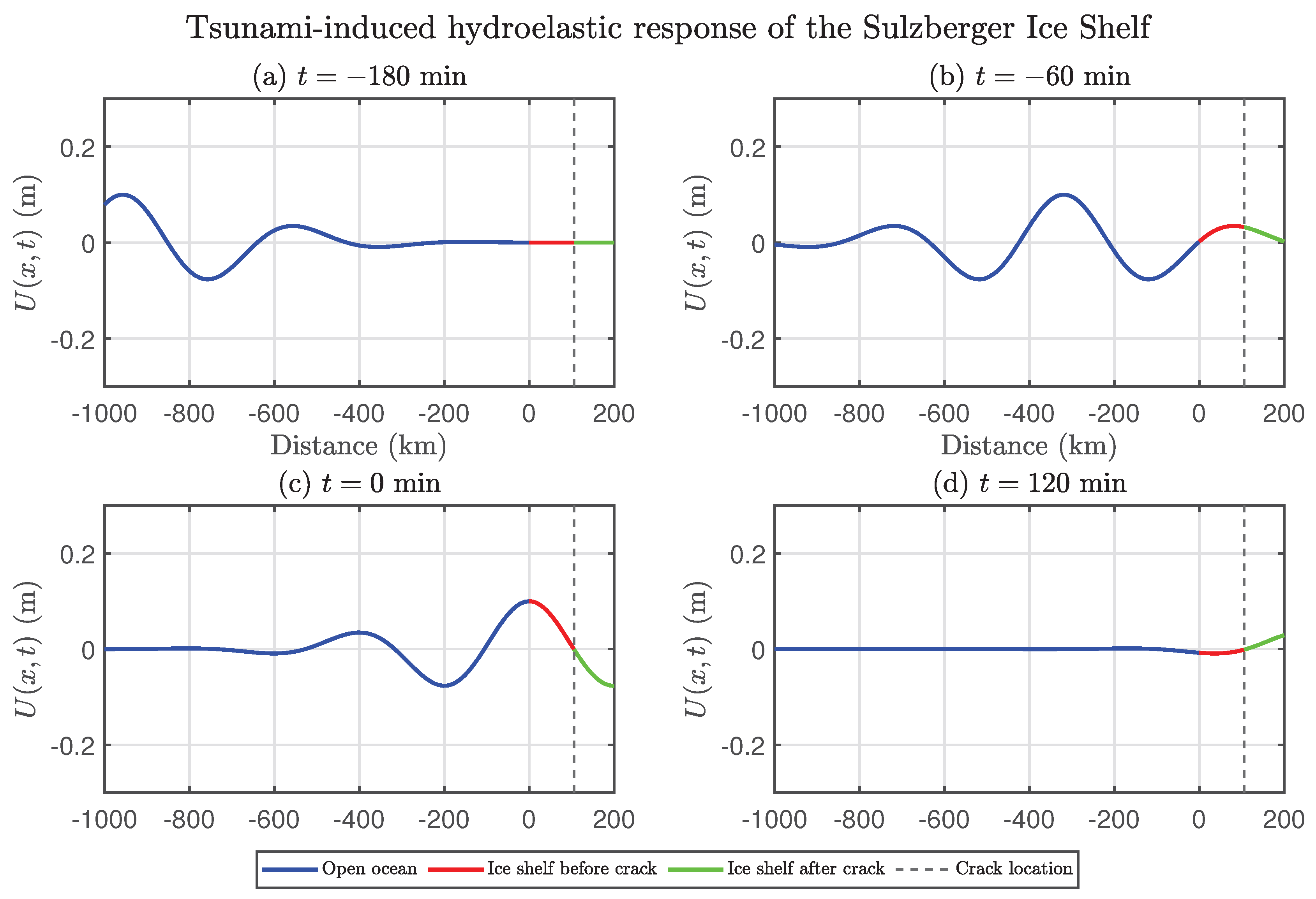
Figure 10.
Time evolution of tsunami wave along the Sulzberger Ice Shelf for low-frequency forcing ( Hz). The wave propagates across the shelf with no reflection.
Figure 10.
Time evolution of tsunami wave along the Sulzberger Ice Shelf for low-frequency forcing ( Hz). The wave propagates across the shelf with no reflection.
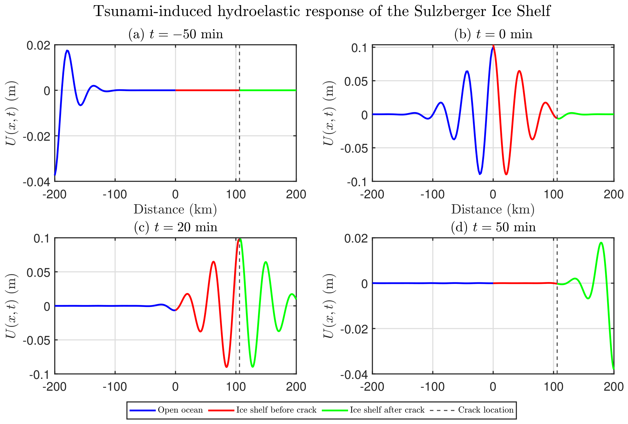
Figure 11.
Time evolution of tsunami wave along the Sulzberger Ice Shelf for higher-frequency forcing ( Hz). The wave reflected and bent at the crack location.
Figure 11.
Time evolution of tsunami wave along the Sulzberger Ice Shelf for higher-frequency forcing ( Hz). The wave reflected and bent at the crack location.
Disclaimer/Publisher’s Note: The statements, opinions and data contained in all publications are solely those of the individual author(s) and contributor(s) and not of MDPI and/or the editor(s). MDPI and/or the editor(s) disclaim responsibility for any injury to people or property resulting from any ideas, methods, instructions or products referred to in the content. |
© 2026 by the authors. Licensee MDPI, Basel, Switzerland. This article is an open access article distributed under the terms and conditions of the Creative Commons Attribution (CC BY) license (http://creativecommons.org/licenses/by/4.0/).
Copyright: This open access article is published under a Creative Commons CC BY 4.0 license, which permit the free download, distribution, and reuse, provided that the author and preprint are cited in any reuse.


