

Submitted:
02 July 2026
Posted:
03 July 2026
You are already at the latest version
Abstract
This study proposes a multi-stage approach to modelling dependencies using Vector Autoregression (VAR), Nonlinear Autoregressive Neural Network (NAR-NN) models, and copulas. This paper aims to assess the dynamic dependency structure between cryptocurrencies and traditional financial assets, considering regime changes and safe-haven properties. The proposed methodology integrates change point detection with copula-based conditional correlation Generalized Autoregressive Conditional Heteroscedasticity (GARCH) models to identify structural breaks and nonlinear de-pendencies between regimes. A sequential change point procedure based on fast signal segmentation is employed to detect structural changes. According to the study, cryp-tocurrencies and traditional assets exhibit regime-dependent dependence. It was also determined that during periods of market stress, this dependency significantly in-creases. This paper has significant implications for portfolio diversification, risk man-agement, and the role of digital assets in financial markets. Furthermore, this proposed methodology contributes to literature by capturing nonlinear, time-dependent, and re-gime-dependent dependency structures.
Keywords:
interconnections
; financial markets
; change point detection
; copula
; VAR
; DCC-GARCH family models
; neural network
1. Introduction
The nonlinear and volatile nature of financial assets makes it difficult to identify their interdependency structure. Many researchers have revealed their complex relationships and their extreme sensitivity to periods of financial stress. Tse and Tsui [1] and Bae et al. [2] have identified the degree of connectivity between markets as a significant factor in contagion analysis. Forbes and Rigobon [3] pointed out that high levels of market dependence can simply be the result of strong links that always persist in turbulent periods; however, the main concern is contagion, i.e., a significant increase in cross-market comovement following a shock. There are important implications for the global economy from contagion in financial markets, including monetary policy, asset allocation, risk measurement, capital adequacy, and asset pricing. These implications have been the subject of many important papers, including Londstaff [4] and Aloui et al. [5]. Several papers have focused on the history of the financial crisis and crisis models [6,7], while others have looked at theoretical models of contagion [8,9]. Generally, studies on contagion tests focus on empirical applications as reported by Bekaert et al. [10], Corsetti et al. [11], Eichengreen et al. [12], Favero and Giavazzi [13].
Cryptocurrencies have created new challenges and opportunities for investors and policymakers in recent years. Cryptocurrency markets are often considered alternatives for portfolio diversification. However, more research is needed to analyze their interdependence on conventional assets since the results of empirical findings remain ambiguous. While some studies in the literature indicate weak correlations on average between cryptocurrencies and traditional assets such as stocks, commodities, and currencies, other findings suggest that these relationships may strengthen during times of crisis, potentially weakening their role as safe-haven assets [14].
Modeling cross-market dependence presents a significant issue in measuring the degree of dependence and in determining the structure of dependence. A classic tool for comparing dependence structures in financial economies is the Pearson (or linear correlation) coefficient. Despite its simplicity, the linear correlation is no longer considered a valid indicator of market dependence due to its static nature and inability to measure average links across markets. A Pearson correlation coefficient only considers linear statistical dependency and requires that the observables have a close-to-normal distribution. Although the central limit theorem may allow this in some circumstances, statistical dependence is often very complex. There are many situations in which a single number cannot capture statistical dependence adequately. The joint probability distribution captures the statistical dependence between the variables and provides a comprehensive understanding of their relationship, but shapes can vary depending on the underlying process involved. Typically, this method cannot be used to compare the statistical dependence of different systems [15]. As a result of its significant limitations, Pearson’s linear correlation is not suited to “heavy-tailed” distributions, particularly in the field of financial economics [16]. Some alternative methods, which rely on traditional correlations, have drawn a lot of criticism for not being able to accurately identify complex dependencies among markets [17].
To investigate cross-market financial dependencies, multivariate GARCH techniques have been recommended [18] as well as copula functions [19]. In the literature, Multivariate GARCH models (MGARCH) have been widely used (see [20,21,22]); for example, the dynamic conditional correlation GARCH-type model [23]. This model considers the impact of the volatility of other markets and can capture the dynamic conditional correlation of the multivariate time series. In addition to multivariate GARCH models, Copulas are useful for investigating nonlinear linkages, prompted by multidimensional dependence in financial markets. Since they can handle asymmetric, non-linear, and tail dependence simultaneously, dependence modeling via copula functions has shown promise [18]. The copula methodology provides great flexibility when simulating interdependence between two markets or risk factors and can be used to model various dependencies. Using copulas, it is possible to express a multivariate distribution as a function of its marginal distributions and make it possible to compound joint distributions when only marginal distributions are known. Moreover, marginal distributions can be generated from various families [24]. However, further investigation is required to determine which copula function is best for enhancing hedging performance [25].
One of the most significant limitations of existing studies is that they treat dependency as either a static phenomenon or one that changes smoothly over time. Furthermore, they fail to adequately account for abrupt structural changes. Policy interventions and macroeconomic shocks can significantly change dependency structures, and therefore, financial markets can be subject to regime changes. At this point, ignoring such structural breaks can lead to misleading conclusions. Previous studies have generally evaluated traditional financial assets and the cryptocurrency market separately, and therefore, clear information on inter-market connections is generally ignored.
To provide clearer information on inter-market connections, this study proposes a comprehensive methodology including change point detection with copula-based dependency modeling. The proposed methodology can capture nonlinear and extreme dependencies across asset classes. Furthermore, it ensures the identification of regime-specific dependency structures. In our multi-stage methodology approach, first, we introduce a VAR-NAR-NN hybrid model, where Vector Autoregression (VAR) and Nonlinear Autoregressive Neural Network (NAR-NN) models are integrated in a unified framework to eliminate serial dependency in data. Then, copula-based conditional correlation GARCH-type models are utilized to capture dependency structures, nonlinear, and asymmetric relationships. Thirdly, a sequential change point detection procedure based on fast signal segmentation is used to identify structural breaks. This proposed multi-stage approach can capture inter-regime dependency dynamics.
The key contribution of this study is as follows. First, a unified analysis of dependency structures is conducted, considering cryptocurrency and traditional asset literature. Change point detection with copula-based modeling is integrated to present a regime-sensitive framework. The final contribution is to present new empirical evidence regarding the stability of safe-haven assets. In this context, different market conditions, highlighting the context-dependent nature of diversification benefits, are evaluated.
2. Literature Review
Copulas are a tool designed to investigate nonlinear linkages, prompted by multidimensional dependence in financial markets. Dependency between financial assets is, in fact, a key component of risk management, asset allocation, portfolio diversification, and financial contagion—the term used to describe the spread of financial crises between countries [26]. It is widely acknowledged that both researchers and market participants, in ascertaining the true structure of dependency between foreign markets, continue to face a difficult and fascinating undertaking. For example, policymakers and investors can enhance their asset pricing for derivatives, forecasting, and portfolio hedging by looking at the structure of dependence between international markets [27].
2.1. Dependence Modeling and Empirical Findings
In the literature, there is a wide range of econometric and computational approaches to modeling dependence structures, such as GARCH-family models, ARIMA, VAR-type specifications, and, more recently, machine learning techniques [28,29,30,31]. However, statistical methodologies have led to varying interpretations and conclusions, making it difficult to generalize findings across different empirical studies. Furthermore, nonlinearity and tail dependence have been evaluated using copula-based frameworks. For instance, Pastpipatkul et al. [32] presented that oil shocks significantly influence stock market activity and exchange rates. In some previous studies, dependence structures are often asymmetric and time-varying, especially during periods of financial stress. In foreign exchange markets, extreme co-movements were reported in [33]. The regime-dependent dependency patterns within BRICS were investigated in [34]. Dependence varies according to market conditions and asset classes [35,36]. However, Kayalar et al. [24] observed that no substantial increase is available in the dependence between oil and stock price returns, like the findings on exchange rates, whereas the Norwegian, Asian, Russian, Chinese, and Indian indices show a considerable decline in this regard. Several studies, including Aloui and Aïssa [28] and Gatfaoui [37], demonstrate that regime shifts particularly influence the dependence of commodity prices, exchange rates, and stock markets. Further evidence of asymmetric and crisis-driven dependence is provided by Nguyen et al. [38], Ghaemi Asl et al. [39], and Wang and Xiao [40], who highlight strong spillovers during recessions and an increase in global interconnectivity.
2.2. Cryptocurrency and Cross-Market Dynamics
Recent research extends dependence analysis to cryptocurrencies and their cross-interaction with traditional financial assets. Generally, they conclude that cryptocurrencies are less dependent on conventional markets. For example, Chemkha et al. [17] and Mili and Bouteska [41] observed a weak dependence and limited co-movement of the tail between crypto assets and major fiat currencies. In the same manner, Gil-Alana et al. [42] presented the bilateral links between cryptocurrencies and stock market indices. The results showed that cryptocurrencies behave as a distinct asset class. It was also determined that relative independence varies over time, becoming increasingly synchronized with broader market movements. During the crisis period, Mensi et al. [43] and Asiri et al. [44] presented the increased interconnectedness between cryptocurrencies and traditional assets during crises. Dependence appears heterogeneous and time-varying in cryptocurrency markets. In [45,46], asymmetric relationships across digital assets were described. Significant co-movements in returns and liquidity across major cryptocurrencies were demonstrated in [47]. The results presented that cryptocurrency markets exhibit both internal and cross-market dynamics.
2.3. Safe-Haven Properties and Geopolitical Risks
Financial assets provide a safe-haven, and therefore, a significant increase can be seen in demand. Due to its ability to withstand economic and political turbulence, gold has historically been regarded as the primary safe-haven. However, along with regime shifts, shocks, and market positions, it has reduced its effectiveness as a hedge, prompting investors to seek alternative options. Although the role of digital assets remains highly debated, they have introduced a new dimension to safe-haven asset choices. Some previous studies presented that gold, oil, and Bitcoin can be useful for hedging, but empirical results are inconsistent across different time periods. For instance, Elie et al. [48] determined that crude oil is a weak safe-haven. On the other hand, Kim et al. [49] presented important interactions between Bitcoin, gold, and equity markets. During a crisis, dependence often increases, putting diversification strategies at risk. Mgadmi et al. [50] presented that they evolve during geopolitical shocks. Mensi et al. [51] presented that gold, and cryptocurrencies move together more during uncertain periods.
2.4. Research Gaps and Contribution
In the literature, various studies on financial dependency are available. However, it suffers from several significant shortcomings. The integration of cryptocurrencies into a unified dependency framework remains limited. Previous studies related to asset classes, methodologies, and geographic contexts are also limited. In most studies, traditional assets or digital assets are generally analyzed separately. Hence, more research is needed to provide comprehensive comparative analysis. The other shortcoming is related to the methodology. Previous studies include static or low-dimensional features, and hence, this limits their ability to grasp the complex, dynamic, and multidimensional nature of modern financial systems. In addition, there is no consensus on model selection and specification. For this reason, the comparability of empirical findings is reduced. There is a growing trend towards hybrid methods that capture the dynamic nature of asset prices and economic conditions. These include time-dependent and regime-switching approaches. Hybrid methods can improve risk management by predicting market changes more accurately.
This paper provides several contributions. First, an integrated analysis of dependency structures is provided across both traditional financial assets and cryptocurrencies. This brings together two branches of literature usually considered separately. Second, a flexible modeling methodology is proposed. It can capture nonlinear, asymmetric, and time-dependent dependencies, accounting for regime changes, for a more accurate representation of financial market interactions. This paper contributes to a more holistic understanding of diversification and safe-haven characteristics in increasingly interconnected financial markets.
3. Methodology
Support vector regression and linear regression are two discriminative regression models that have been effectively used for many regression tasks; in some cases, they have even attained state-of-the-art performance. Although these models are effective, they are generally based on the assumption that explanatory variables contribute independently to the response and don’t explicitly account for covariate dependence. Moreover, traditional regression approaches may encounter challenges when dealing with high-dimensional feature spaces, particularly when variables are interdependent. Copula-based models offer an alternative means. Specifically, the Gaussian copula model proposes a flexible method for solving the issues, without relying on priors for stochastic variables; it can model their correlations. Further, Gaussian copula models scale to high dimensions at low computational cost [52]. Selecting a copula function that is unaffected by the marginal distributions of each random variable allows one to describe statistical dependence structures. Copulas can be used for a wide range of statistical dependence modeling tasks because they don’t require the use of a normal distribution assumption or a linearity assumption [53].
In the context of time series modelling, previous studies have examined both Vector Autoregressive (VAR) models and neural networks to capture temporal and nonlinear relationships [54,55]. However, most common approaches consider a neural network after linear filtering through a residual analysis, implying that nonlinear dynamics are treated as a secondary correction to the linear specification. The proposed hybrid model uses a VAR-based extension to capture dependencies by integrating the neural network component into the mean equation. This generates a unified VAR-NAR-NN specification, in which linear and nonlinear dynamics are jointly modeled. This unified formulation is consistent with the Universal Differential Equations framework, which combines known system dynamics with data-driven neural network components.
3.1. A VAR–NAR Neural Network (VAR–NAR-NN) Hybrid Model
To examine time-series relationships between variables and capture market dependencies, VAR models are particularly useful. VAR models incorporate lagged values of multiple time series and use information from related variables to measure the dynamic transmission of shocks between different markets.
Let denote an -dimensional vector of stationary series:
The linear dependence structure can be modelled with a VAR(p) process:
where is a vector of constants, are coefficient matrices, and is the vector of innovations.
The VAR model effectively captures linear dynamic interdependence and propagation effects between variables. However, it does not account for nonlinear dynamics or higher-order, time-dependent dependencies. To overcome this limitation, nonlinear structures can be modeled using Nonlinear Autoregressive Neural Networks (NAR-NN). Using training data for the neural network allows the network to learn optimal weights and approximate predicted complex patterns in data [56]. Initially, the network is trained in an open-loop environment. Using actual observed values as input provides high accuracy during training. After training is complete, the model is converted into a closed-loop system, in which the predicted values are returned as input to multi-step prediction [57].
A NAR-NN can be given as [45]:
where denotes a neural network, represents the lag order, and is the error process.
In this paper, a hybrid methodology is proposed by combining a Vector Autoregressive (VAR) model with a neural network specification. The proposed methodology divides the conditional mean represented by into two parts: a linear component that captures inter-asset interactions and a nonlinear component that accounts for more complex dynamic relationships.
The hybrid model is specified as follows:
In this model, NAR-NN is used to integrate the nonlinear autoregressive component. As a result, the model can capture nonlinear interactions between past observations and preserve the conditional mean’s autoregressive structure. The hybrid methodology captures richer temporal dynamics, such as regime-dependent continuity and asymmetric responses commonly observed in financial markets. Furthermore, the proposed model more effectively filters out nonlinear autoregressive components from the conditional mean, reducing residual nonlinear dependence that might otherwise manifest as misleading time-varying correlations in Dynamic Conditional Correlation (DCC) models.
3.2. Conditional Copula Models
In multivariate time series, VAR and copula models represent two fundamentally different approaches to modeling dependency. Copula models define dependency at the level of co-distribution by linking marginal distributions through a copula function, while VAR specifications define dependency through dynamic interactions in conditional means. Copula models explicitly separate marginal behavior from cross-sectional dependency, allowing for flexible marginal distributions and nonlinear dependency structures. To analyze the dependency structure between variables and to provide flexibility in modeling individual marginal distributions, a conditional Gaussian copula model is used in this paper. This method is particularly useful for scenarios where variables exhibit different behaviors but are interdependent, allowing for a more nuanced understanding of their interactions. Integrating copula techniques is helpful for the analysis of complex financial systems with diverse and evolving dependencies.
A copula is a multivariate distribution function with uniformly distributed marginals that are defined on the unit . For a bivariate copula, is equal to two. The relationship between the function and its marginal distribution functions, and is denoted by the copula function. Copula models are theoretically based on Sklar’s theorem [58]. According to Sklar’s [58], any multivariate joint distribution can be divided into its marginal distributions and linked by copula functions:
where C is the copula function describing the dependence structure between the two variables.
Equation 4 can be generalized for a set of n random variables:
We consider Fi(yi) = ui with
From the Differentiation of equation 5, we obtain the multivariate joint density:
The multivariate function is called the copula, transforming the variables yi into uniform random variables. As marginal values are removed from this transformation, the copula only presents the dependency mechanism between random variables. In financial applications, this property is particularly useful because financial assets often exhibit different marginal behaviors, such as skewness, kurtosis, and volatility clustering. Thus, copula models provide a more flexible theoretical framework, separating marginals from dependence, for analyzing nonlinear and time-varying relationships between financial series.
Let , the n-dimensional standardized normal distribution function with correlation matrix R, the Gaussian copula CG can be defined by:
where .
Patton [59] extended this traditional static copula approach by allowing the dependence structure to evolve dynamically over time, which leads to a modification of equation 7 as:
With , the dependence parameter, which varies over time.
Instead of assuming constant dependence parameters, the copula becomes conditional on the information set available at time , denoted by . The multivariate conditional joint density can therefore be written as:
The conditional density function of the Gaussian copula is obtained by:
where |Rt| is the determinant of the correlation matrix, with , the standard normal cumulative distribution function, and I, the identity matrix. One of the main contributions of Patton is introducing conditional copulas according to autoregressive dynamics, close to GARCH-type models.
3.3. Conditional Correlation Models
Conditional correlation GARCH-type models provide an effective method for modeling volatility dynamics and correlation of time series. This study employs copula-based multivariate GARCH family models to examine the dependence structure among financial asset returns. A copula can be integrated into a conditional GARCH framework by retaining univariate GARCH models for each marginal series and replacing the linear correlation structure component with a time-varying copula. By combining the properties of copulas in modeling joint distributions with the dynamic correlation GARCH-type models, the copula DCC-GARCH model is particularly relevant in finance to capture market stress conditions. The GARCH specification (exponential generalized autoregressive conditional heteroskedasticity (EGARCH) and DCC-EGARCH) can be improved by accounting for volatility asymmetry [60,61].
The standard dynamic conditional correlation model (DCC-GARCH) in Engle [23] decomposes the conditional covariance matrix. of equation 1, as follows:
where Rt is the conditional correlation matrix and
, the matrix elements of standard deviations for each data series obtained from estimating a univariate GARCH-type process.
To modeling time varying dependence, Patton’s methodology can be combined with the dynamic conditional correlation models. The conditional covariance process can be written as:
where is the unconditional covariance matrix of the standardized residuals obtained from a GARCH-type process.
a and b, the constant parameters, reflect the sensitivity of recent shocks and persistence from past correlations, respectively.
Conditions on parameters are: .
should be normalized to obtain the dynamic conditional correlation matrix :
A further analysis is to evaluate the time-varying nature of correlations. The selection of the appropriate conditional model is essential. This helps us to determine whether correlations remain stable or fluctuate in different economic contexts, ensuring insights into the dynamic nature of financial dependencies and improving the robustness of correlation-based analyses. To this end, we compare the Constant Conditional Correlation GARCH (CCC-GARCH) model with the Dynamic Conditional Correlation GARCH (DCC-GARCH) model. The CCC-GARCH model, originally introduced by Bollerslev [62], is a multivariate framework. It allows for time-varying conditional variances while assuming that correlations remain constant over time. Under this assumption, the conditional correlation matrix is time-invariant.
In the literature, Engle and Sheppard [63] and likelihood ratio tests are widely used to compare the CCC-GARCH and DCC-GARCH specifications. However, both approaches present important limitations, particularly for our study. The likelihood ratio test is sensitive to model misspecification and relies on strong distributional assumptions, essentially regarding the correct specification of the multivariate GARCH structure. The Engle–Sheppard test, although specifically designed to detect time variation in correlations, depends on standardized residuals and may suffer from low power in small samples. To overcome these limitations, we additionally propose a Weighted Dynamic Dependency Index (WDDI) test, defined as a weighted sum of the absolute autocorrelations of residual cross-products across several lags.
For a pair of assets , let , the autocorrelation of the cross-product at lag .
The WDDI index is defined as:
where = .
To summarize dependence across all pairs:
where is the number of asset pairs.
Unlike standard approaches that rely on hypothesis testing procedures or model-implied parameters, the WDDI provides a simple and model-free scalar summary of residual dependence based on the autocorrelations of cross-products. This index uses decreasing weights to higher-order lags, considering short-run dependence dynamics, which are most relevant for conditional correlation modeling. In this sense, the WDDI complements existing diagnostic tools by quantifying the magnitude of persistence rather than simply testing for its presence. The WDDI index provides a more informative assessment of model adequacy before the estimation of multivariate conditional correlation models.
3.4. Change-Point Detection and Regime Identification
A change-point detection analysis enables investors to identify regime shifts to adapt their portfolio management strategies. Recent studies highlight the importance of identifying structural breaks in dynamic markets and change point detection methods are increasingly being applied to financial and economic data [64,65]. Traditional solutions for detecting changes in parameters such as mean or variance rely on probability-based frameworks and cumulative sum (CUSUM) techniques. Furthermore, studies in literature focus on detecting multiple change points and overcoming the challenges associated with high-dimensional or non-parametric data: for example, through exact cost-penalty optimization strategies such as wild binary segmentation [66] and PELT [67]. Extensive research has been conducted on various methodologies, including offline density ratio-based approaches [68]. Other approaches based on alternative principles have been developed to detect distributional changes in time-ordered data.
This study uses the Energy distance method to identify market change points across stock markets, gold, and bitcoin, and to highlight inter-market connections. This method relies on energy statistics to measure the differences between distributions before and after potential change points, making it sensitive to general changes in location, scale, and dependency structures without requiring a parametric specification.
Let the sample of data, be partitioned into two segments (Xt, Yt) at a candidate break point :
such that the data before and after follow different distributions:
when and when
F and G denote the cumulative distribution functions associated with the two distributions.
The difference between two segments can be measured using energy statistics ( [76]:
where and are identical and independent distributed copies of X and Y, respectively, α is a fixed constant satisfying 0 < α <2, and denotes the Euclidean norm.
Energy distance provides a non-parametric method for measuring the difference between probability distributions based on pairwise Euclidean distances between observations. Specifically, it is defined as a function of the expected distances within and between samples. However, it is equal to zero if the underlying distributions are identical. Unlike traditional parametric approaches, energy statistics can capture general distributional differences, including changes in higher-order moments and tail behavior, an important feature for financial time series analysis. Energy distance can be utilized to compare adjacent segments of a data series in the context of change point detection. At this point, significant increases indicate the presence of structural breaks and regime changes.
By maximizing the divergence between possible segmentations, a sample version of the energy statistic is measured, and change points are identified [69]:
In the identification of multiple change points, a single change-point detection procedure is repeatedly applied. This iterative process can be represented as a binary tree. It begins with the full time series as the root node, corresponding to a dataset with no detected change points. The most significant change point within a segment is identified at each stage. The segment is divided accordingly, producing two child nodes. This process recursively expands the tree structure, extending each resulting segment. This continues until additional significant change points are determined or the segments become too small to allow for further splitting.
4. Empirical Analysis
In time series analysis, the observation of gradual or abrupt changes in the distribution of data over time gives a better understanding of different phases within the data. It can also enable the creation of prediction models specifically designed for each segment. As a result, overall prediction performance improves because the models can be fine-tuned according to the specific characteristics of each segment. In statistical analysis, the change point problem deals with the analysis of situations where observations exhibit different distributions before and after a certain temporal threshold. Recent studies highlight the importance of identifying structural breaks in dynamic markets and increasingly apply change point detection methods to financial and economic data. In this study, the E-splitting method is used to identify market change points across stock markets, gold, and bitcoin, and highlight inter-market connections.
4.1. Data Analysis
We investigate the dependence of stock markets, Gold, and Bitcoin, selecting a sample dataset for each asset class from January 2018 to December 2024. The daily closing prices are collected from FRED. As the closing price series represented by pt are non-stationary, the series are transformed into log-differentiated series. The choice of log returns, rt, is motivated by the strong rejection of the Phillips-Perron test for unit roots for all the data series included in our analysis1.
The nonparametric multiple-change-point detection method is applied to the return series. This approach assumes that the returns are independent and possess finite α-th absolute moments for some α in the interval (0,2). According to the recommendation of [69], the default value of 1 is used.
A minimum-maximum scaling method is used to normalize the logarithmic returns of the multivariate data series context. The minimum-maximum scaling method ensured that all data points were evaluated on the same scale. This method preserves data distributional properties, which facilitate the comparison between various asset classes and improve our change-point detection accuracy. Figure 1a presents the evolution of the data series and returns, as well as the multiple change points identified through hierarchical split estimation. The red dashed lines represent the change points, providing a clear view of the evolution of the data.
Our analysis identified three common dates: February 24, 2020, April 2, 2020, and October 20, 2021. We can observe that these dates are likely to correspond to significant events or trends in economies. For example, February 24, 2020, coincides with the date when the COVID-19 pandemic’s impact on markets and economies was globally acknowledged. April 2, 2020, may signal further adjustments as economic policies are implemented to mitigate the pandemic effects. October 20, 2021, may indicate market recovery and renewed investor confidence as economies begin to reopen, thus impacting financial markets. Figure 1b shows each data series separately, along with the three previously identified turning shifts.
As a result of the pandemic crisis, all data series experienced a significant decline between February and April 2020, but a quick recovery, as shown in Figure 1b. During this period, the Dow Jones Industrial Index, S&P 500, and Nasdaq Composite Index reached their highest values in September 2021. In contrast, Bitcoin reached two of its highest values in September 2020, followed by a second peak in September 2021. Furthermore, all volatility trends exhibit similar dynamics over time, except that gold has shown a continuous upward trend since the pandemic period. This can be explained by gold’s traditional role as a safe-haven asset during periods of economic uncertainty and high market volatility. Following the pandemic, Figure 4b shows a general upward trend across all data series starting in 2022. This trend has been maintained and reached its highest level in 2024.
To analyze the distinct role played by Gold and Bitcoin during this period, and to show how Bitcoin’s and gold’s statistical properties have changed significantly over time, we estimate multiple change points for gold and Bitcoin univariate time series. From Figure 1c, we observe one change point in gold in June 2019, and two in Bitcoin in December 2020 and July 2022.
In response to the pandemic crisis, we noticed a strong interest in gold and bitcoin. To better understand the nature and strength of asset dynamics, we incorporate macroeconomic variables into the analysis. Macroeconomic indicators can provide some insights into how external events have influenced economic performance and investor behavior. Figure 2 shows the connection between gold prices and federal funds rates during the pandemic crisis. The shift in gold prices in June 2019 can be explained by low interest rates and expansionary monetary policies during the pandemic. This is likely to increase demand for gold as a hedge against inflation. Traditionally, low interest rates increase the attractiveness of interest-free assets like gold. Furthermore, inflationary tensions observed from 2020 onwards have driven investors towards gold as a hedge against potential value loss. At this point, investors use gold as a popular option to protect their capital.
In the same manner, monetary policy has played a significant role in the adoption of cryptocurrencies compared to traditional financial instruments. Bitcoin’s exchange rate in December 2020 can be attributed to increasing institutional investor interest in Bitcoin as an asset class. Investors seek alternative investments during this period due to economic uncertainty and fiscal stimulus. Cryptocurrencies are also often seen as a hedge against potential monetary instability, but traditional financial systems have become more volatile. Bitcoin’s exchange rate in July 2022 appears to have experienced the highest inflation rate at that time, while dependence of Bitcoin on speculative transactions and exposure to macroeconomic factors make it a highly volatile and unpredictable asset.
In this paper, the observation period is divided into three distinct and economically significant phases. Gradual increases in interest rates characterize the pre-pandemic monetary policy during 2018-2019. Afterward, the pandemic period (2020–2021) is during which interest rates reaching their historically low levels in response to severe economic disruption and increased uncertainty. Finally, the post-pandemic period (from 2022 to 2024) presents a significant rise in interest rates aimed at containing inflationary pressures. This temporal segmentation reflects the structural changes in macroeconomic conditions and policy regimes caused by the pandemic, fundamentally altering financial market dynamics. To evaluate the evolving relationships between traditional financial assets and digital assets, these periods ensure a robust and theoretically grounded framework.
Descriptive statistics of returns data series are reported according to the sub-periods previously identified, and are given respectively in Table 1, Table 2 and Table 3.
The return is higher during the pandemic period 2020-2021, according to the comparison results of the average return over the periods for all investments. It was observed that before COVID-19, Bitcoin returns were negative but became higher compared to other investments during the COVID-19 crisis period. For the last period, all the returns decreased except for Gold, and all investments had a lower variability than before. For all investments, the return volatility is substantially the same.
It was determined that the difference between the maximum and minimum returns for Bitcoin is the highest in each period. Thus, Bitcoin has experienced more significant fluctuations relative to other markets. Bitcoin remained the riskiest asset with more negative extreme values after the COVID-19 pandemic. The high volatility and speculative nature of cryptocurrencies often exacerbate the connection between stock financial markets and cryptocurrencies [75]. In recent studies, Bitcoin and stock assets have shown a low level of connection, particularly during the non-crisis period, while during periods of market stress, the connectedness increases, indicating financial contagion between markets [61,70].
4.2. A VAR-Based Connectedness Analysis
Before estimating the VAR-NAR-NN hybrid model, a VAR-based connectedness study is conducted to obtain preliminary results of the interdependence structure across financial assets. This first study is particularly useful for motivating the VAR-NAR-NN framework, which can capture more complex and nonlinear interactions that are beyond the scope of conventional VAR models. Furthermore, a VAR-based connectedness analysis allows the identification of contagion, spillovers, and the visualization of the connection structure of the markets [71,72,73,74]. This method is based on forecast error variance decomposition. It identifies how much one asset’s forecast error variance is explained by shocks from another asset. By analyzing the dynamic relationships between multiple time series, this method helps identify the direction and intensity of connections among markets. It provides a quantitative measure of how intertwined different financial markets are, especially during times of economic uncertainty.
Following the Ljung-Box test results for autocorrelation (Appendix A) and the Schwarz information criterion, we consider a VAR process of order 1 to study the relationship between variables and market correlations. Based on the variance decompositions on 20-step-ahead forecasts, we report the connectedness measures for the three distinct and economically significant periods (Table 4, Table 5 and Table 6).
The Total Connectedness Index (TCI) has revealed a moderate to strong contagion between markets. This index increased during the pandemic crisis from 49.55% in 2018-2019 to 58.74% and continued to rise, reaching 59.38% in 2022-2024. The pandemic amplified global stock market interconnectedness, highlighting how external shocks were able to intensify market linkages. As a result, the pandemic period saw stock markets become more sensitive to each other’s movements. From 2022 to 2024, SP500 contributed to the highest variance in forecast error by transmitting 78.65%, followed by the Nasdaq at 71.5 %, and the Dow Jones at 65.74 %. Further, these conventional markets experienced the highest spillovers between them: S&P 500 at 60.28%, Nasdaq at 57.44. %, and Dow Jones at 55.77.68% (2022-2024). On the other hand, in the same period, 93.47% of the future variance of gold and 64.28 % of the future variance of bitcoin come from their own shocks. Before the pandemic, this percentage was 98.14 % for Bitcoin, reflecting the total disconnection of Bitcoin from conventional assets. In periods 2 and 3, we observe that Gold’s contributions remained the lowest, 4.24% and 1.46%, respectively, confirming its status as a safe-haven asset. Over the pandemic period, Bitcoin’s contribution to others increased, reaching 20.18% in the last period.
Network representations from Figure 3. provide an intuitive interpretation of how shocks are transmitted across markets over time. Graphically, we can observe the parts of the highest variance contributions in forecast error, of all assets. The size of each node in the connectedness figures reflects the magnitude of risk each market transmits or receives. A larger node corresponds to more risk volume, and thicker lines between nodes indicate greater risk flow from one market to another.
Figure 3 shows that the SP500, DJIA, and Nasdaq (except before the pandemic) were net transmitters of risk to others (represented in blue), with the SP500 the greatest transmitter. At the same time, Gold and Bitcoin were the net receivers (depicted in yellow). Dynamic net pairwise connectedness indicates that Bitcoin was disconnected before the pandemic crisis. There has been an increase in contagion effects during the pandemic period, particularly an increase in variance transmission in Gold and Bitcoin, indicating that markets have become highly interconnected. During the crisis, Gold became the main receiver, but after the crisis, Bitcoin received the most spillovers, especially from the SP500 and the Nasdaq. Its increased risk contribution to other assets presents its growing influence and potential as a hedge or speculative asset. During times of economic uncertainty, investors considered Bitcoin as a more volatile but potentially higher-return asset compared to Gold.
In shaping cross-market asset interactions, macroeconomic signals play a significant role. Under different economic conditions, understanding regime-dependent connections provides insights into how assets behave. This knowledge provides more informed decisions about portfolio adjustments and identifies opportunities for diversification and risk management.
5. Results and Discussions
Linkage dynamics derived from the predictive variance decompositions of the VAR model form the basis for analyzing inter-market interdependencies and spillover effects. On the other hand, the presence of nonlinear interactions is not sufficiently captured by VAR linear dynamics. This motivates the proposed hybrid model in this study based on equation 3. Specifically, the hybrid model incorporates NAR-NN with lagged inputs to approximate a first-order nonlinear autoregressive component [77]. Residual dependencies in correlations are analyzed by modelling the VAR-NAR-NN residuals in a copula-based DCC-EGARCH framework. As an initial step, the residuals of the VAR–NAR-NN model are tested for heteroscedasticity. The results, reported in Appendix B, include multivariate Ljung–Box tests applied to the squared residuals, revealing significant autocorrelation across all three sub-periods. The findings indicate conditional heteroscedasticity, requiring volatility models for each asset. Finally, to assess alternative dependence structures, we compare a copula-based Constant Conditional Correlation EGARCH model with its dynamic extension.
5.1. Testing Conditional Correlation Models
In this analysis, we will compare conditional correlation models to determine whether a time-varying correlation structure can better reflect the joint behavior of asset returns, especially during calms and crises. Table 7 shows the results of the p-value of the Likelihood Ratio (LR) and the Engle-Sheppard (ES) tests:
Both the likelihood ratio tests and the Engle–Sheppard tests yield consistent evidence regarding the temporal dependence structure in the first period. However, for the remaining two periods, the results are less conclusive. In the second period, the Engle–Sheppard tests indicate time-varying correlations when applied with lag orders of 5 and 10, whereas tests with lag orders of 1 and 5 suggest the presence of constant correlations for the last period.
In addition to these statistical tests, we present a heatmap of cross-product autocorrelations across standardized residuals (Figure 4) to visualize the dependence dynamics between asset pairs. This graphical approach helps detect localized dependence patterns that may not be captured by global multivariate tests. The heatmap summarizes autocorrelation values across both pairs and lags in a single representation, allowing heterogeneous correlation persistence to be easily identified. In the following graphs, the autocorrelation functions of cross-products are reported up to 10 lags to assess the short-run correlation dynamics. The following heatmaps reveal strong correlation persistence in asset pairs, for specific lags. This heterogeneity helps explain why pairwise diagnostics detect dynamic dependence in the last period even though the global DCC test does not reject constant correlation.
Figure 4.
Cross-product autocorrelations of standardized residuals.
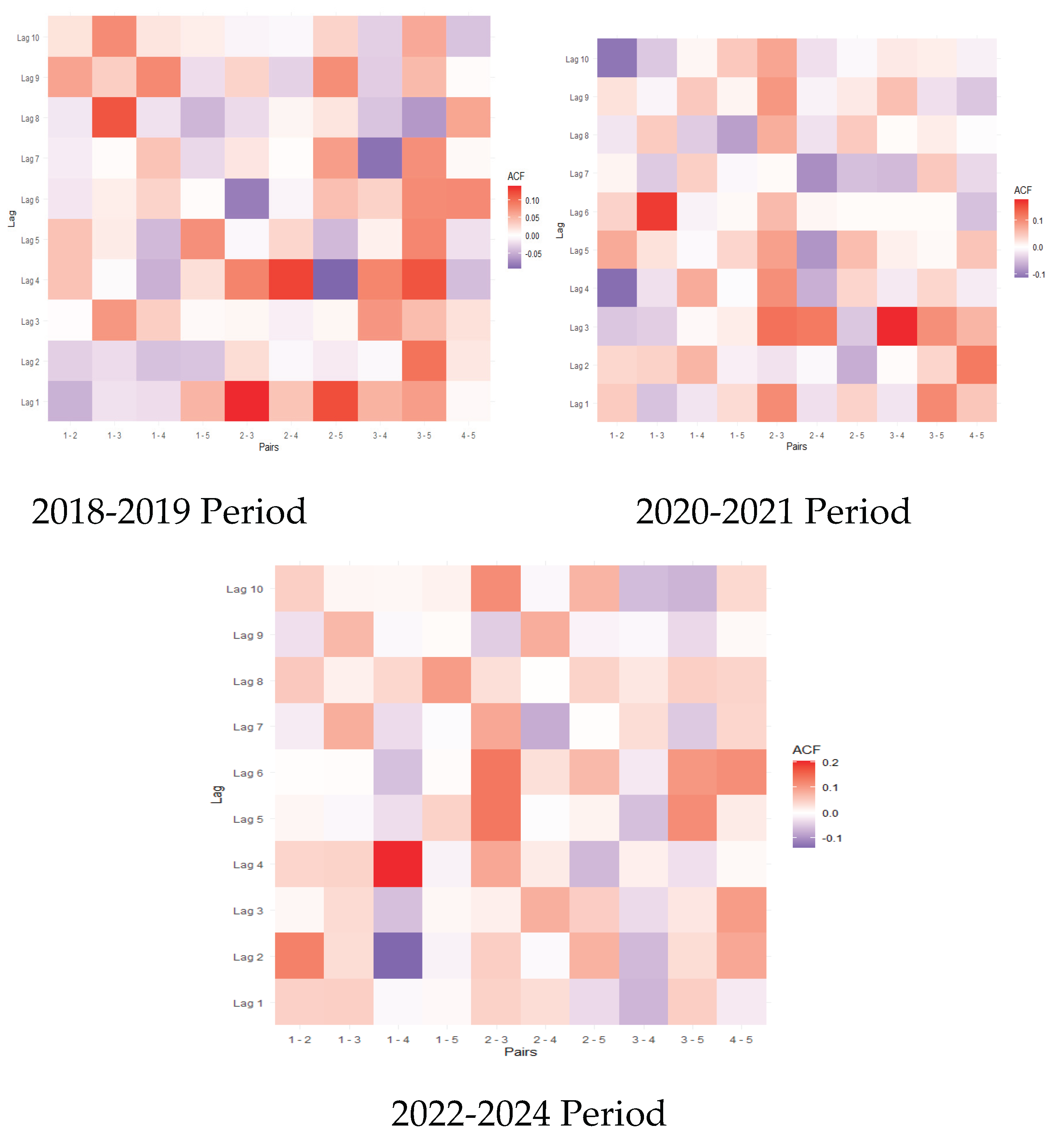
More specifically, to quantify correlation persistence, we report in Table 8 the estimations of the WDDI index for orders 5 and 10.
From Table 8, we observe a reduction in the index in the standardized residuals of the copula DCC EGARCH model for the three periods.
5.2. Empirical Findings
In this study, a unified approach is proposed combining linear VAR modeling, nonlinear neural autoregressive dynamics, and a copula-based dynamic conditional correlation EGARCH model to comprehensively capture linear, nonlinear, and time-varying dependence structures. The multivariate dependence structure is modeled using a Gaussian copula, while heavy tails are captured at the marginal level via Student-t-EGARCH innovations. The following tables give the results of the dynamic conditional correlation models for each sub-period.

Table 9.
The model results for the period 2018-2019.
| Assets | Coefficient | P-Value |
| GOLD α | 0.0664 | 0.0121 |
| β | 0.9649 | 0.0000 |
| γ | 0.1038 | 0.0000 |
| Shape | 10.111 | 0.0097 |
| SP500 α | -0.2468 | 0.0000 |
| β | 0.9567 | 0.0000 |
| γ | 0.0585 | 0.0445 |
| Shape | 6.0583 | 0.0000 |
| DJIA α | -0.2260 | 0.0000 |
| β | 0.9532 | 0.0000 |
| γ | 0.0874 | 0.0000 |
| Shape | 5.8843 | 0.000 |
| BITCOIN α | -0.0048 | 0.9028 |
| β | 0.9813 | 0.0000 |
| γ | 0.3502 | 0.0000 |
| Shape | 2.6364 | 0.0000 |
| NASDAQ α | -0.2347 | 0.0000 |
| β | 0.9550 | 0.0000 |
| γ | 0.0524 | 0.0241 |
| Shape | 7.4623 | 0.0000 |
| αDCC | 0.0426 | 0.0000 |
| βDCC | 0.8816 | 0.0000 |
Table 10.
The model results for the period 2020-2021.
| Assets | Coefficient | P-Value |
| GOLD α | 0.0439 | 0.1229 |
| β | 0.9634 | 0.0000 |
| γ | 0.0655 | 0.000 |
| Shape | 5.1012 | 0.000 |
| SP500 α | -0.1029 | 0.0348 |
| β | 0.9241 | 0.0000 |
| γ | 0.4566 | 0.0011 |
| Shape | 6.5775 | 0.0019 |
| DJIA α | -0.0104 | 0.0102 |
| β | 0.9460 | 0.0000 |
| γ | 0.3550 | 0.0116 |
| Shape | 6.1899 | 0.0016 |
| BITCOIN α | 0.0263 | 0.1897 |
| β | 0.9887 | 0.0000 |
| γ | 0.1264 | 0.0066 |
| Shape | 3.4101 | 0.0000 |
| NASDAQ α | -0.1105 | 0.0042 |
| β | 0.9486 | 0.0000 |
| γ | 0.2912 | 0.0011 |
| Shape | 4.5535 | 0.0000 |
| αDCC | 0.0437 | 0.0000 |
| βDCC | 0.8779 | 0.0000 |
Table 11.
The model results for the period 2022-2024.
| Assets | Coefficient | P-Value |
| GOLD α | 0.1402 | 0.0244 |
| β | 0.7522 | 0.0000 |
| γ | 0.0091 | 0.8645 |
| Shape | 5.8426 | 0.0000 |
| SP500 α | -0.1038 | 0.0000 |
| β | 0.9858 | 0.0000 |
| γ | 0.0412 | 0.0000 |
| Shape | 26. 2521 | 0.2968 |
| DJIA α | -0.0634 | 0.0001 |
| β | 0.9921 | 0.0000 |
| γ | 0.0625 | 0.0000 |
| Shape | 17.3381 | 0.1306 |
| BITCOIN α | 0.0286 | 0.3462 |
| β | 0.9850 | 0.0000 |
| γ | 0.1197 | 0.3659 |
| Shape | 2.8431 | 0.0000 |
| NASDAQ α | -0.0886 | 0.0000 |
| β | 0.9884 | 0.0000 |
| γ | 0.0120 | 0.0375 |
| Shape | 99.9417 | 0.0374 |
| αDCC | 0.0237 | 0.000 |
| βDCC | 0.9618 | 0.000 |
Based on the tables, the Copula-DCC-EGARCH model is validated, since all the joint coefficients αDCC and βDCC that represent the conditional correlation parameters are significant, regardless of the period considered. The sum of these coefficients reflects the persistence of the conditional correlation. For the three periods, the persistence of the conditional correlation exceeded 0.9. Furthermore, the models are validated, verifying no autocorrelation in the standardized residuals (see Appendix C).
We observe that most of the coefficients are significant in the variance equation, especially concerning the first (before COVID) period. The α coefficients from the variance equation are not significant for some data series. Bitcoin in all periods and Gold in the second period can be given as examples. Furthermore, the high persistence between markets is confirmed since β coefficients are always significantly positive. Except in the last period for Bitcoin and Gold, the leverage effect is significant for all data series. To determine the values of the conditional correlation for pairs of series, the estimation of the Copula-DCC-EGARCH model parameters can be used. The strength of the relationship between the two series is indicated by the correlation values for a particular pair of series.
Table 12, Table 13 and Table 14 present the means of conditional correlations. The results showed that the tail behavior of Bitcoin, Gold, and the stock market index are very similar regarding contemporaneous correlation. In addition, the conditional correlation between Bitcoin and stock markets has increased from 2022 to 2024, especially with Nasdaq, reaching 0.399, confirming Bitcoin’s adaptability to economic conditions. Despite this, Gold and Bitcoin had the lowest conditional correlation of any period, suggesting that they can be used as hedges against stock indices. For conventional assets, the conditional correlation is above 0.9. The highest correlation occurs between the SP500 and the Dow Jones during the period of crisis, and between the SP500 and the Nasdaq for the last period.
Figure 5 and Figure 6, Figure 7, Figure 8 and Figure 9 illustrate the dynamics of the relationship for the three periods of observation.
Figure 5 illustrates the downward trend in the dependence between the SP500 and Dow Jones after the pandemic. In the meantime, the SP500 and Nasdaq have increased their dependence (Figure 6), with the highest correlation in March 2023 (above 0.97). The differing effects of technological progress and economic recovery on diverse sectors can explain this shift in dependence. In the post-pandemic period, Nasdaq benefited more from the increased demand for digital solutions. On the other hand, the Dow Jones has experienced a slower recovery, leading to a decrease in its correlation with the SP500.
Conditional correlations between SP500 and Bitcoin, sometimes negative during the first period, have consistently been positive from the pandemic crisis period, with values generally below 0.5. Figure 7 shows that the most positive conditional correlation values were obtained during the pandemic in March 2020, and frequently in 2022, with values above 0.5. These results have been consistent with the transmission of macroeconomic signals influencing the correlation between these two classes of assets. In contrast, correlations between Gold and the SP500 reached their most negative levels during the COVID-19 pandemic (Figure 8), supporting the general results that gold returns are inversely proportional to stock market conditions.
Figure 9 highlights the divergence between Bitcoin and Gold correlations, more pronounced immediately before the start of the COVID-19 pandemic and from 2021. As an example, its highest negative peak (-0.2) was reached in late 2021. Results indicate that Bitcoin and Gold have reacted differently to market conditions over time. Gold may have moved independently of, or even in the opposite direction of, the situation. The negative correlation in late 2021 reflected Bitcoin’s unique status as a digital asset.
6. Conclusion
In recent years, cryptocurrency markets have gained popularity in financial markets. Because of the success of Bitcoin, many other cryptocurrencies have emerged, stimulating innovation and competition. Their decentralized nature and widespread use give an alternative to traditional financial systems. Blockchain-based projects are becoming more popular, increasing confidence in currency models. Due to their multifaceted systems, evaluating the connections between the stock market, the gold market, and the cryptocurrency market is quite complex.
This paper develops a novel methodology to analyze the evolving relationships between different asset classes. The proposed VAR-NAR-NN can identify and model complex nonlinear relationships within time series data, and it ensures a nuanced approach to predicting financial assets. The proposed Copula DCC-EGARCH model can capture time-dependent correlations and understand the dynamic relationships between financial assets. Furthermore, directional dependency analysis is more robust because of the integration of the Gaussian copula. On the one hand, the VAR-NAR-NN model offers an in-depth look at nonlinear dependencies. On the other hand, the Copula DCC-EGARCH model provides clarity in correlation analysis, complementing each other in a comprehensive financial analysis. The results of the study showed that the regime-dependent connections between bitcoin and conventional assets are highly dependent on structural breaks. Bitcoin can fluctuate unpredictably in response to macroeconomic changes, such as shifts in interest rates and geopolitical tensions, which both increase its volatility. This may affect its perceived stability and attractiveness as a safe-haven asset.
Findings showed that Bitcoin and gold play different roles as preventative or reactive assets against index movement crises. Bitcoin generally tends to exhibit higher volatility and can act as a leading indicator during crises. However, gold often functions as a safe-haven asset, maintaining or increasing its value while traditional markets experience declines. This interaction suggests that gold remains a preferred option for those prioritizing stability and wealth preservation during turbulent economic times, while Bitcoin can be attractive to risk-tolerant investors seeking high returns. Investors might consider diversifying their portfolios to include both Bitcoin and gold to balance risk and capitalize on their differing responses to market conditions.
It has been shown that macroeconomic indicators have a great impact on cross-market connections, providing early signals. Early signals can be useful for some investors to prepare for potential financial turbulence and lead them to determine alternative assets as a hedge against potential market instability. In this paper, proposed models can be utilized to develop more robust portfolio diversification strategies, enabling investors to reduce risks by including both traditional and cryptocurrency assets. Additionally, financial institutions can use these results to enhance risk assessment models and ensure better predictions and responses to market fluctuations. Furthermore, trading decisions can be optimized by these models based on inter-market relationships.
The pandemic reshaped traditional financial systems, accelerating digital currencies and adopting technologies. To remain competitive, these changes forced banks to innovate and integrate blockchain technology. Examining how emerging cryptocurrencies’ interactions with traditional stock markets exhibit long-term stability or volatility can be considered in future research. Furthermore, how regulatory changes in the cryptocurrency market influence stock market behavior can give valuable insights. One of the main future challenges for cryptocurrencies is the extent of artificial intelligence (AI) in the transformation of the financial sector. As artificial intelligence can greatly enhance blockchain technology, it brings with it the environmental and energy demands of large-scale AI and blockchain systems. As such, future innovation will not only depend on improving performance and profitability, but also on developing more energy-efficient algorithms and reducing the ecological footprint of AI-powered blockchains.
Author Contributions
Conceptualization, V.T. and A.B.İ.; methodology, V.T. and A.B.İ.; software, V.T. and A.B.İ.; validation, V.T; investigation, V.T. and A.B.İ.; data curation, V.T; writing—original draft preparation, V.T. and A.B.İ.; writing—review and editing, V.T. and A.B.İ.; visualization, V.T; supervision, V.T. All authors have read and agreed to the published version of the manuscript.
Funding
This research received no external funding.
Institutional Review Board Statement
Not applicable.
Informed Consent Statement
Not applicable.
Data Availability Statement
The datasets used and analyzed during the current study are available from the corresponding author upon reasonable request.
Acknowledgments
The authors would like to express acknowledgment to Antonia Margherita, Research Development Specialist in the DEM at the University of Luxembourg, for her contribution and collaborative spirit throughout this research study. This paper is a revised and expanded version of a paper entitled ‘Regime Dependent Dependence: Cryptocurrencies and Traditional Assets under Structural Breaks’ presented at La 5e Journée d’Économétrie Appliquée Michel Terraza, Montpellier, France, 29 May 2026.
Conflicts of Interest
The authors declare no conflicts of interest.
Appendix A
Appendix A shows tests for autocorrelation in the returns using the Ljung-Box test.
Table A1, Table A2 and Table A3 report the Q-Statistic and P-value for Bitcoin, gold, and the stock market indexes.
Table A1.
Q-Statistic and P-value for return series (period 1).
| Series | Q-Statistic | P-value |
| GOLD | 15.425 | 0.219 |
| SP500 | 10.919 | 0.5359 |
| DJIA | 8.7184 | 0.7268 |
| BITCOIN | 8.607 | 0.7361 |
| NASDAQ | 11.688 | 0.471 |
Table A2.
Q-Statistic and P-value for return series (period 2).
| Series | Q-Statistic | P-value |
| GOLD | 34.909 | 0.000 |
| SP500 | 232.01 | < 2.2e-16 |
| DJIA | 234.05 | < 2.2e-16 |
| BITCOIN | 23.827 | 0.021 |
| NASDAQ | 164.93 | < 2.2e-16 |
Table A3.
Q-Statistic and P-value for return series (period 3).
| Series | Q-Statistic | P-value |
| GOLD | 11.37 | 0.497 |
| SP500 | 13.916 | 0.306 |
| DJIA | 9.954 | 0.62 |
| BITCOIN | 13.36 | 0.343 |
| NASDAQ | 18.317 | 0.106 |
Appendix B
Autocorrelation test in the square of the residuals of the VAR –NAR-NN (1) model using the multivariate Ljung Box test. (lag=12)
| Periods | Q-statistics | P-value |
| Period 1 | 527 | 0 |
| Period 2 | 1734 | 0 |
| Period 3 | 588.5 | 0 |
Appendix C
Appendix C reports tests for autocorrelation in the Standardized residuals of the Copula DCC EGARCH model using the Ljung Box test. Table C1, Table C2 and Table C3 give the Q-Statistic and P-value according to the period.
Table C1.
Q-Statistic and P-value for standardized residuals (period 1).
| Series | Q-Statistic | P-value |
| GOLD | 14.197 | 0.1642 |
| SP500 | 6.3309 | 0.7867 |
| DJIA | 7.8642 | 0.6421 |
| BITCOIN | 12.698 | 0.2411 |
| NASDAQ | 31.196 | 0.0000 |
Table C2.
Q-Statistic and P-value for standardized residuals (period 2).
| Series | Q-Statistic | P-value |
| GOLD | 18.853 | 0.0043 |
| SP500 | 5.6335 | 0.8451 |
| DJIA | 9.9956 | 0.4409 |
| BITCOIN | 16.504 | 0.0861 |
| NASDAQ | 11.201 | 0.3421 |
Table C3.
Q-Statistic and P-value for standardized residuals (period 3).
| Series | Q-Statistic | P-value |
| GOLD | 9.1567 | 0.5173 |
| SP500 | 10.599 | 0.3896 |
| DJIA | 9.6175 | 0.4747 |
| BITCOIN | 4.2868 | 0.9335 |
| NASDAQ | 8.101 | 0.6190 |
| 1 | Details on the test and tables showing the results are omitted for the sake of brevity. This can be requested from the authors. |
| 2 | “From” indicates the measure of the directional connectedness that a given asset receives the shocks from all other assets. |
| 3 | indicates the measure of the directional connectedness that a given asset transmits its shock to all other assets. |
| 4 | TCI indicates the total connectedness. |
| 5 | means the difference between the two-directional connectedness. |
References
- Tse; Tsui, Y. K. A. K. C. A multivariate GARCH model with time-varying correlations. J. Bus. Econ. Stat. 2002, 20, 351–362. [Google Scholar]
- Bae, K.H.; Karolyi; G.A. Stulz, R.M. A new approach to measuring financial contagion. Rev. Financ. Stud. 2003, 16(3), 717–763. [Google Scholar] [CrossRef]
- Forbes, K.; Rigobon, R. No contagion, only interdependence: measuring stock market co-movements. J. Financ. 2002, 57(5), 2223–2261. [Google Scholar]
- Londstaff, F. The subprime credit crisis and contagion in financial markets. J. Financ. Econ. 2010, 97(3), 436–450. [Google Scholar] [CrossRef]
- Aloui, R.; Aïssa, M. S. B.; Nguyen, D. K. Global financial crisis, extreme interdependences, and contagion effects: The role of economic structure? J. Bank. Financ. 2011, 35(1), 130–141. [Google Scholar] [CrossRef]
- Bordo, M.; Murshid, A. Are financial crises becoming increasingly more contagious? What is the evidence on contagion. Working paper, 2000. [Google Scholar]
- Kaminsky, G.L.; Reinhart, C.M. Financial markets in times of stress. NBER Working Paper, #8569, 2001. [Google Scholar]
- Calvo, S.; Mendoza, E. Rational contagion and the globalization of securities markets. J. Int. Econ. 2000, 51, 79–113. [Google Scholar] [CrossRef]
- Kodres, L.E.; Pritsker, M. A rational expectations model of financial contagion. J. Financ. 2002, 57(2), 768–799. [Google Scholar] [CrossRef]
- Bekaert, G.; Harvey, C.R.; Ng, A. Market integration and contagion. J. Bus. 2005, 78(1), 39–69. [Google Scholar] [CrossRef]
- Corsetti, G.; Pericoli, M.; Sbracia, M. Some Contagion, Some Interdependence: More Pitfalls in Tests of Financial Contagion. J. Int. Money Financ. 2005, 24. [Google Scholar] [CrossRef]
- Eichengreen, B.; Rose, A.K.; Wyplosz, C. Contagious currency crises. NBER Work. Pap. 5681 1996. [Google Scholar] [CrossRef]
- Favero, C.A.; Giavazzi, F. Is the international propagation of financial shocks non-linear? Evidence from the ERM. J. Int. Econ. 2002, 57(1), 231–246. [Google Scholar]
- Li, L.; Miu, P. Are cryptocurrencies a safe haven for stock investors? A regime-switching approach. J. Empir. Financ. 2023, 70, 367–385. [Google Scholar]
- Münnix, M. C.; Schäfer, R. A copula approach on the dynamics of statistical dependencies in the US stock market. Phys. A Stat. Mech. Appl. 2011, 390(23-24), 4251–4259. [Google Scholar] [CrossRef]
- Tibprasorn, P.; Autchariyapanitkul, K.; Chaniam, S.; Sriboonchitta, S. A copula-based stochastic frontier model for financial pricing. Integrated Uncertainty in Knowledge Modelling and Decision Making: 4th International Symposium, IUKM 2015, Nha Trang, Vietnam, October 15-17, 2015; Springer International Publishing; Proceedings 4, pp. 151–162. [Google Scholar]
- Chemkha, R.; BenSaïda, A.; Ghorbel, A. Connectedness between cryptocurrencies and foreign exchange markets: Implication for risk management. J. Multinatl. Financ. Manag. 2021, 59, 100666. [Google Scholar] [CrossRef]
- Ab Razak, R.; Ismail, N. Dependence modeling and portfolio risk estimation using GARCH-copula approach. Sains Malays. 2019, 48(7), 1547–1555. [Google Scholar] [CrossRef]
- BenSaïda, A.; Boubaker, S.; Nguyen, D. K. The shifting dependence dynamics between the G7 stock markets. Quant. Financ. 2018, 18(5), 801–812. [Google Scholar]
- Bollerslev, T.; Engle, R.; Wooldridge, J. A Capital Asset Pricing Model with Time-Varying Covariances. J. Polit. Econ. 1988, 96(1), 116–31. [Google Scholar] [CrossRef]
- Ng, L. Tests of the CAPM with time-varying covariances: A multivariate GARCH approach. J. Financ. 1991, 46, 1507–1521. [Google Scholar] [CrossRef]
- Hansson, B.; Hordahl, P. Testing the conditional CAPM using multivariate GARCH. Appl. Financ. Econ. 1998, 8, 377–388. [Google Scholar] [CrossRef]
- Engle, R. F. Dynamic conditional correlation: A simple class of multivariate generalized autoregressive conditional heteroskedasticity models. J. Bus. Econ. Stat. 2002, 20(3), 339–350. [Google Scholar]
- Kayalar, D. E.; Küçüközmen, C. C.; Selcuk-Kestel, A. S. The impact of crude oil prices on financial market indicators: copula approach. Energy Econ. 2017, 61, 162–173. [Google Scholar] [CrossRef]
- Lai, Y.; Chen, C. W.; Gerlach, R. Optimal dynamic hedging via copula-threshold-GARCH models. Math. Comput. Simul. 2009, 79(8), 2609–2624. [Google Scholar]
- BenSaïda, A. The contagion effect in European sovereign debt markets: A regime-switching vine copula approach. Int. Rev. Financ. Anal. 2018, 58, 153–165. [Google Scholar] [CrossRef]
- Charfeddine, L.; Benlagha, N. A time-varying copula approach for modelling dependency: New evidence from commodity and stock markets. J. Multinatl. Financ. Manag. 2016, 37, 168–189. [Google Scholar] [CrossRef]
- Aloui, R.; Aïssa, M. S. B. Relationship between oil, stock prices and exchange rates: A vine copula based GARCH method. N. Am. J. Econ. Financ. 2016, 37, 458–471. [Google Scholar] [CrossRef]
- Hsieh, C. H.; Huang, S. C. Time-varying dependency and structural changes in currency markets. Emerg. Mark. Financ. Trade 2012, 48(2), 94–127. [Google Scholar] [CrossRef]
- Doman, M.; Doman, R. Dependencies between stock markets during the period including the late-2000s financial crisis. Procedia Econ. Financ. 2012, 1, 108–117. [Google Scholar] [CrossRef]
- Xu, J.; Cao, L. Copula Variational LSTM for High-dimensional Cross-market Multivariate Dependence Modeling. arXiv 2023, arXiv:2305.08778. [Google Scholar]
- Pastpipatkul, P.; Yamaka, W.; Sriboonchitta, S. Co-movement and dependency between New York stock exchange, London stock exchange, Tokyo stock exchange, oil price, and gold price. In Integrated Uncertainty in Knowledge Modelling and Decision Making: 4th International Symposium, IUKM 2015; Nha Trang, Vietnam, Proceedings, Ed.; Springer International Publishing, 15-17 October 2015; Volume 4, pp. 362–373. [Google Scholar]
- Albulescu, C. T.; Aubin, C.; Goyeau, D.; Tiwari, A. K. Extreme co-movements and dependencies among major international exchange rates: A copula approach. Q. Rev. Econ. Financ. 2018, 69, 56–69. [Google Scholar] [CrossRef]
- Kumar, S.; Tiwari, A. K.; Chauhan, Y.; Ji, Q. Dependence structure between the BRICS foreign exchange and stock markets using the dependence-switching copula approach. Int. Rev. Financ. Anal. 2019, 63, 273–284. [Google Scholar] [CrossRef]
- Li, J.; Li, P. Empirical analysis of the dynamic dependence between WTI oil and Chinese energy stocks. Energy Econ. 2021, 93, 104299. [Google Scholar] [CrossRef]
- Abakah, E. J. A.; Addo, E., Jr.; Gil-Alana, L. A.; Tiwari, A. K. Re-examination of international bond market dependence: Evidence from a pair copula approach. Int. Rev. Financ. Anal. 2021, 74, 101678. [Google Scholar] [CrossRef]
- Gatfaoui, H. Linking the gas and oil markets with the stock market: Investigating the US relationship. Energy Econ. 2016, 53, 5–16. [Google Scholar] [CrossRef]
- Nguyen, C.; Bhatti, M. I.; Henry, D. Are Vietnam and Chinese stock markets out of the US contagion effect in extreme events? Phys. A Stat. Mech. Appl. 2017, 480, 10–21. [Google Scholar] [CrossRef]
- Ghaemi Asl, M.; Tavakkoli, H. R.; Rashidi, M. M. Sector-by-sector analysis of dependence dynamics between global large-cap companies and infectious diseases: A time-varying copula approach in EBOV and COVID-19 episodes. PLoS ONE 2021, 16(11), e0259282. [Google Scholar] [PubMed]
- Wang, B.; Yang; Xiao, Y. Risk spillovers from China’s and the US stock markets during high-volatility periods: Evidence from East Asian stock markets. Int. Rev. Financ. Anal. 2023, 86. [Google Scholar]
- Mili, M.; Bouteska, A. Forecasting nonlinear dependency between cryptocurrencies and foreign exchange markets using dynamic copula: evidence from GAS models. J. Risk Financ. 2023, 24(4), 464–482. [Google Scholar]
- Gil-Alana, L. A.; Abakah, E. J. A.; Rojo, M. F. R. Cryptocurrencies and stock market indices. Are they related? Res. Int. Bus. Financ. 2020, 51, 101063. [Google Scholar] [CrossRef]
- Mensi, W.; Hanif, W.; Bouri, E.; Vo, X. V. Spillovers and tail dependence between oil and US sectoral stock markets before and during COVID-19 pandemic. Int. J. Emerg. Mark. 2024, 19(11), 4155–4185. [Google Scholar]
- Asiri, A.; Alnemer, M.; Bhatti, M. I. Interconnectedness of Cryptocurrency Uncertainty Indices with Returns and Volatility in Financial Assets during COVID-19. J. Risk Financ. Manag. 2023, 16(10), 428. [Google Scholar] [CrossRef]
- Hyun, S.; Lee, J.; Kim, J. M.; Jun, C. What coins lead in the cryptocurrency market: using Copula and neural networks models. J. Risk Financ. Manag. 2019, 12(3), 132. [Google Scholar] [CrossRef]
- Huang, C. C.; Hsu, C. C. Evaluating dependence between DeFi tokens and conventional cryptocurrencies. Appl. Econ. Lett. 2024, 32(7), 1–7. [Google Scholar] [CrossRef]
- Zhang, M.; Zhu, B.; Li, Z.; Jin, S.; Xia, Y. Relationships among return and liquidity of cryptocurrencies. Financ. Innov. 2024, 10(1). [Google Scholar] [CrossRef]
- Elie, B.; Naji, J.; Dutta, A.; Uddin, G. S. Gold and crude oil as safe-haven assets for clean energy stock indices: Blended copulas approach. Energy 2019, 178, 544–553. [Google Scholar] [CrossRef]
- Kim, J. M.; Kim, S. T.; Kim, S. On the relationship of cryptocurrency price with us stock and gold price using copula models. Mathematics 2020, 8(11), 1859. [Google Scholar] [CrossRef]
- Mgadmi, N.; Sadraoui, T.; Alkaabi, W.; Abidi, A. The interconnectedness of stock indices and cryptocurrencies during the Russia-Ukraine war. J. Econ. Criminol. 2023, 2, 100039. [Google Scholar] [CrossRef]
- Mensi, W.; El Khoury, R.; Ali, S. R. M.; Vo, X. V.; Kang, S. H. Quantile dependencies and connectedness between the gold and cryptocurrency markets: Effects of the COVID-19 crisis. Res. Int. Bus. Financ. 2023, 65, 101929. [Google Scholar] [CrossRef]
- Duan, J.; Ding, X.; Liu, T. A Gaussian copula regression model for movie box-office revenues prediction. Sci. China Inf. Sci. 2017, 60(9), 1–14. [Google Scholar] [CrossRef]
- Kim, J. M.; Lee, N.; Xiao, X. Directional dependence between major cities in China based on copula regression on air pollution measurements. PLoS ONE 2019, 14(3), e0213148. [Google Scholar] [CrossRef] [PubMed]
- Parot, A.; Michell, K.; Kristjanpolle, W. D Using Artificial Neural Networks to forecast Exchange Rate, including VAR-VECM residual analysis and prediction linear combination. Intell. Syst. Account. Financ. Manag. 2019, 26(1), 3–15. [Google Scholar]
- Rahman, A.; Upadhye, N. Hybrid Vector Auto Regression and Neural Network Model for Order Flow Imbalance Prediction in High Frequency Trading. arXiv 2024. [Google Scholar]
- Kırbaş, İ.; Sözen, A.; Tuncer, A. D.; Kazancıoğlu, F. Ş. Comparative analysis and forecasting of COVID-19 cases in various European countries with ARIMA, NARNN and LSTM approaches. Chaos Solit. Fractals. 2020, 138, 110015. [Google Scholar] [CrossRef]
- Benrhmach, G.; Namir, K.; Namir, A.; Bouyaghroumni, J. Nonlinear autoregressive neural network and extended Kalman filters for prediction of financial time series. J. Appl. Math. 2020, 1–6. [Google Scholar] [CrossRef]
- Sklar, A. Fonctions de répartition à n dimensions et leurs marges. Publ. De l’Institut De Stat. De l’Université De Paris 1959, 8, 229–231. [Google Scholar]
- Patton, A.J. Modelling Asymmetric Exchange Rate Dependence. Int. Econ. Rev. 2006, 47(2), 527–556. [Google Scholar] [CrossRef]
- Nelson, D.B. Conditional Heteroskedasticity in Asset Returns: A New Approach. Econometrica 1991, 59(2), 347–370. [Google Scholar] [CrossRef]
- Terraza, V.; Boru İpek, A.; Rounaghi, M.M. The nexus between the volatility of Bitcoin, gold, and American stock markets during the COVID-19 pandemic: Evidence from VAR-DCC-EGARCH and ANN models. Financ. Innov. 2024, 10(22). [Google Scholar]
- Bollerslev, T. Modelling the Coherence in Short-Run Nominal Exchange Rates: A Multivariate Generalized Arch Model. Rev. Econ. Stat. 1990, 72(3), 498–505. [Google Scholar] [CrossRef]
- Engle, R. F.; Sheppard, K. NBER Working Paper No. 8554; Theoretical and Empirical Properties of Dynamic Conditional Correlation Multivariate GARCH. National Bureau of Economic Research, October 2001.
- Banerjee, S.; Guhathakurta, K. Change point analysis in financial networks. Stat 2020, 9(1), e269. [Google Scholar] [CrossRef]
- Boubaker, S.; Liu, Z.; Sui, T.; Zhai, L. The mirror of history: How to statistically identify stock market bubble bursts. J. Econ. Behav. Organ. 2022, 204, 128–147. [Google Scholar] [CrossRef]
- Fryzlewicz, P. WBS: Wild Binary Segmentation for Multiple Change-Point Detection. Ann. Stat. 2014, 42, 2243–2281. [Google Scholar]
- Killick, R.; Fearnhead, P.; Eckley, I. A. Optimal detection of changepoints with a linear computational cost. J. Am. Stat. Assoc. 2012, 107(500), 1590–1598. [Google Scholar] [CrossRef]
- Truong, C.; Oudre, L.; Vayatis, N. Selective Review of Offline Change Point Detection Methods. Article ID: 107299; Signal Process. 2020; 167. [Google Scholar]
- Matteson, D. S.; James, N. A. A nonparametric approach for multiple change point analysis of multivariate data. J. Am. Stat. Assoc. 2014, 109(505), 334–345. [Google Scholar] [CrossRef]
- Attarzadeh, A.; Balcilar, M. On the dynamic return and volatility connectedness of cryptocurrency, crude oil, clean energy, and stock markets: a time-varying analysis. Environ. Sci. Pollut. Res. 2022, 29(43), 65185–65196. [Google Scholar] [CrossRef]
- Diebold, F. X.; Yilmaz, K. Better to Give than to Receive: Predictive Measurement of Volatility Spillovers (with discussion). Int. J. Forecast. 2012, 28, 57–66. [Google Scholar]
- Diebold, F.X.; Yilmaz, K. On the Network Topology of Variance Decompositions: Measuring the Connectedness of Financial Firms. J. Econom. 2014, 182, 119–134. [Google Scholar] [CrossRef]
- Diebold, F. X.; Yilmaz, K. On the past, present, and future of the Diebold–Yilmaz approach to dynamic network connectedness. J. Econom. 2023, 234, 115–120. [Google Scholar] [CrossRef]
- Buchwalter, B.; Diebold, F. X.; Yilmaz, K. Clustered network connectedness: a new measurement framework with application to global equity markets. J. Econom. 2026, 106243. [Google Scholar]
- Kumar, A.; Iqbal, N.; Mitra, S. K.; Kristoufek, L.; Bouri, E. Connectedness among major cryptocurrencies in standard times and during the COVID-19 outbreak. J. Int. Financ. Mark. Inst. Money. 2022, 77, 101523. [Google Scholar] [CrossRef]
- Székely Gábor, J.; Rizzo Maria, L. Energy statistics: A class of statistics based on distances. J. Stat. Plan. Inference 2013, 143(8), 1249–1272. [Google Scholar] [CrossRef]
- Terraza, V.; Boru İpek, A. Regime Dependent Dependence: Cryptocurrencies and Traditional Assets under Structural Breaks’. La 5e Journée d’Économétrie Appliquée Michel Terraza, Montpellier, France, 29 May 2026. [Google Scholar]
Figure 1a.
Change-point detection of multivariate data series.
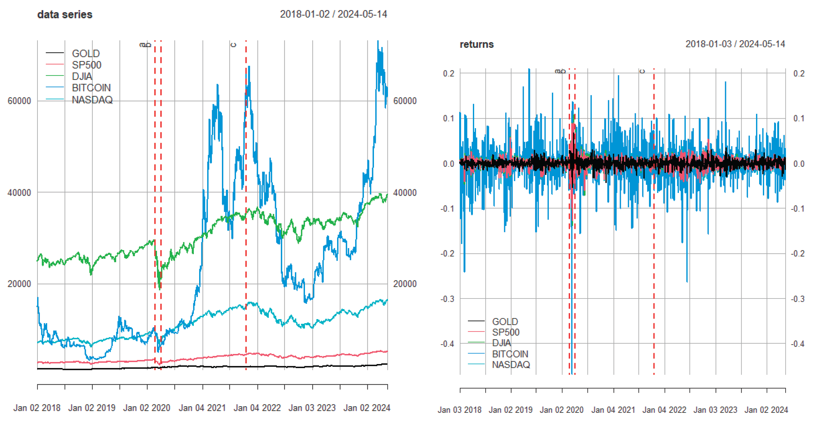
Figure 1b.
Evolution of Assets and Returns.
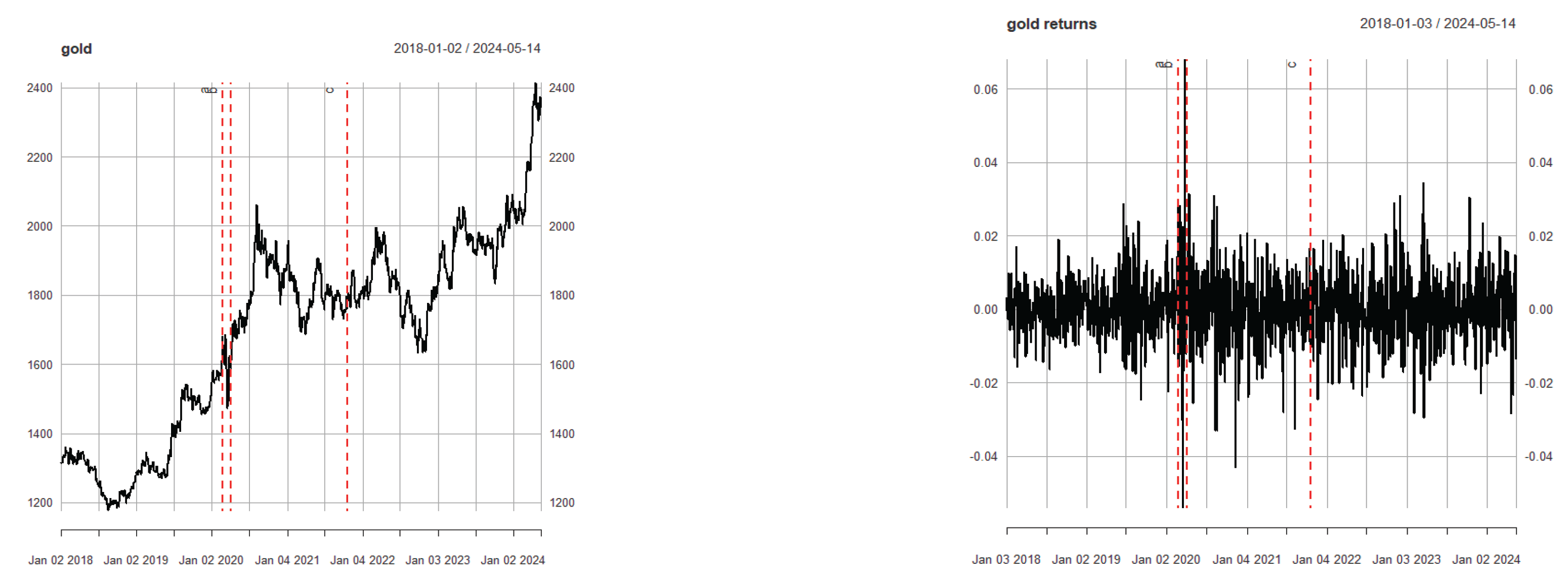
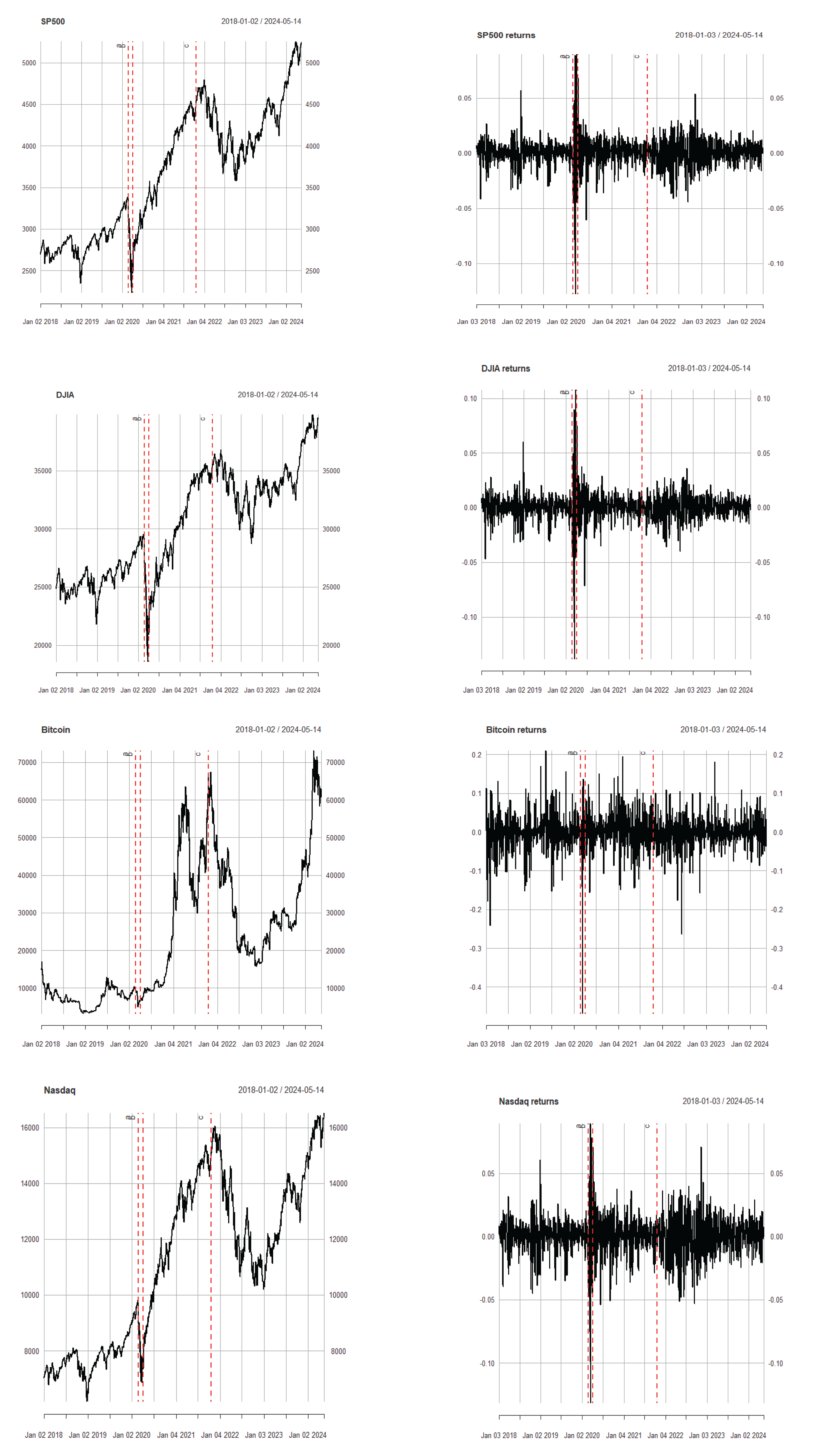
Figure 1c.
Change-point detection for gold and Bitcoin.
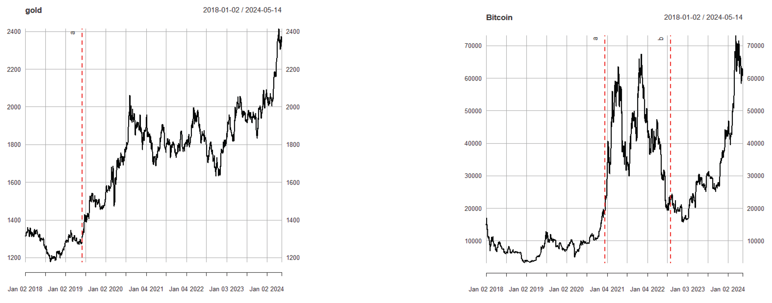
Figure 2.
Macroeconomic indicators.
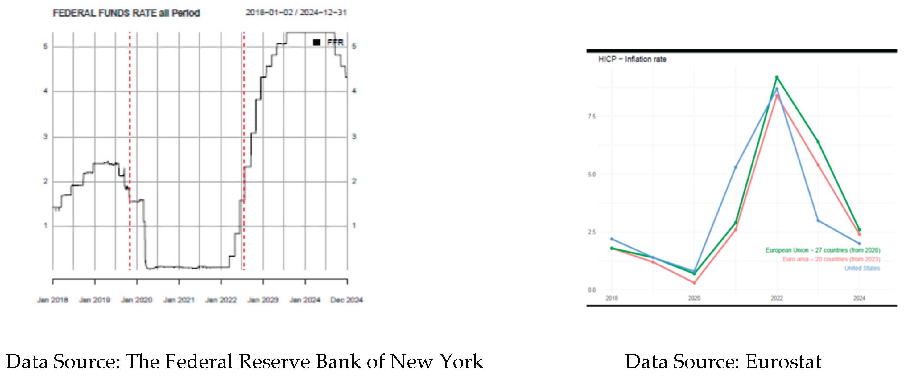
Figure 3.
Connectedness between financial markets.
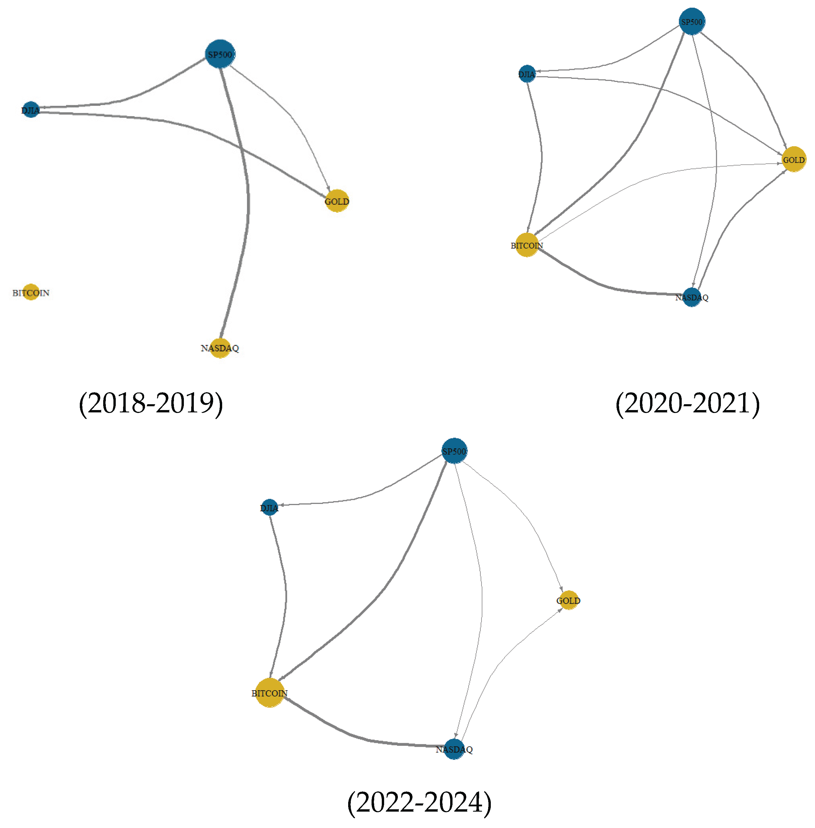
Figure 5.
Conditional correlation of the SP500 with the Dow Jones over the 3 periods.
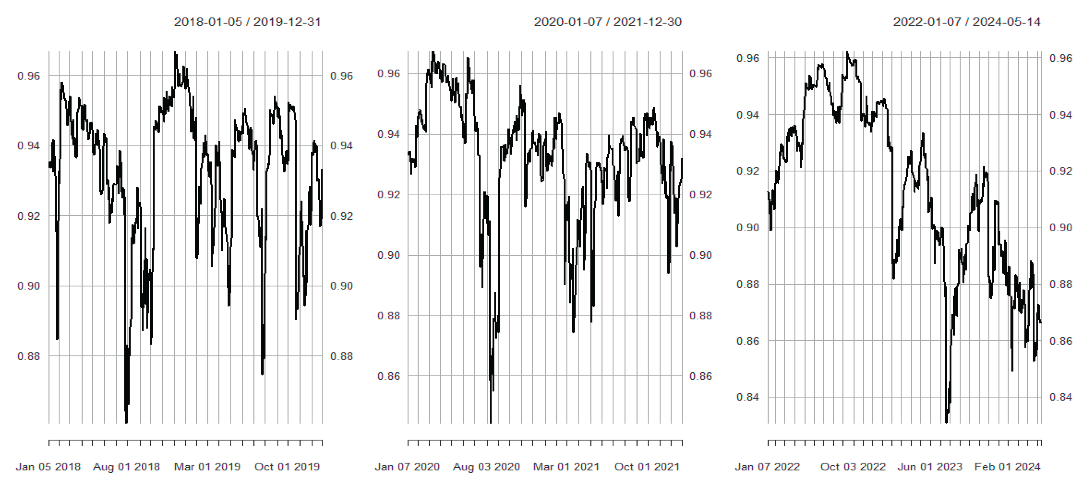
Figure 6.
Conditional correlation of the SP500 with the Nasdaq over the 3 periods.
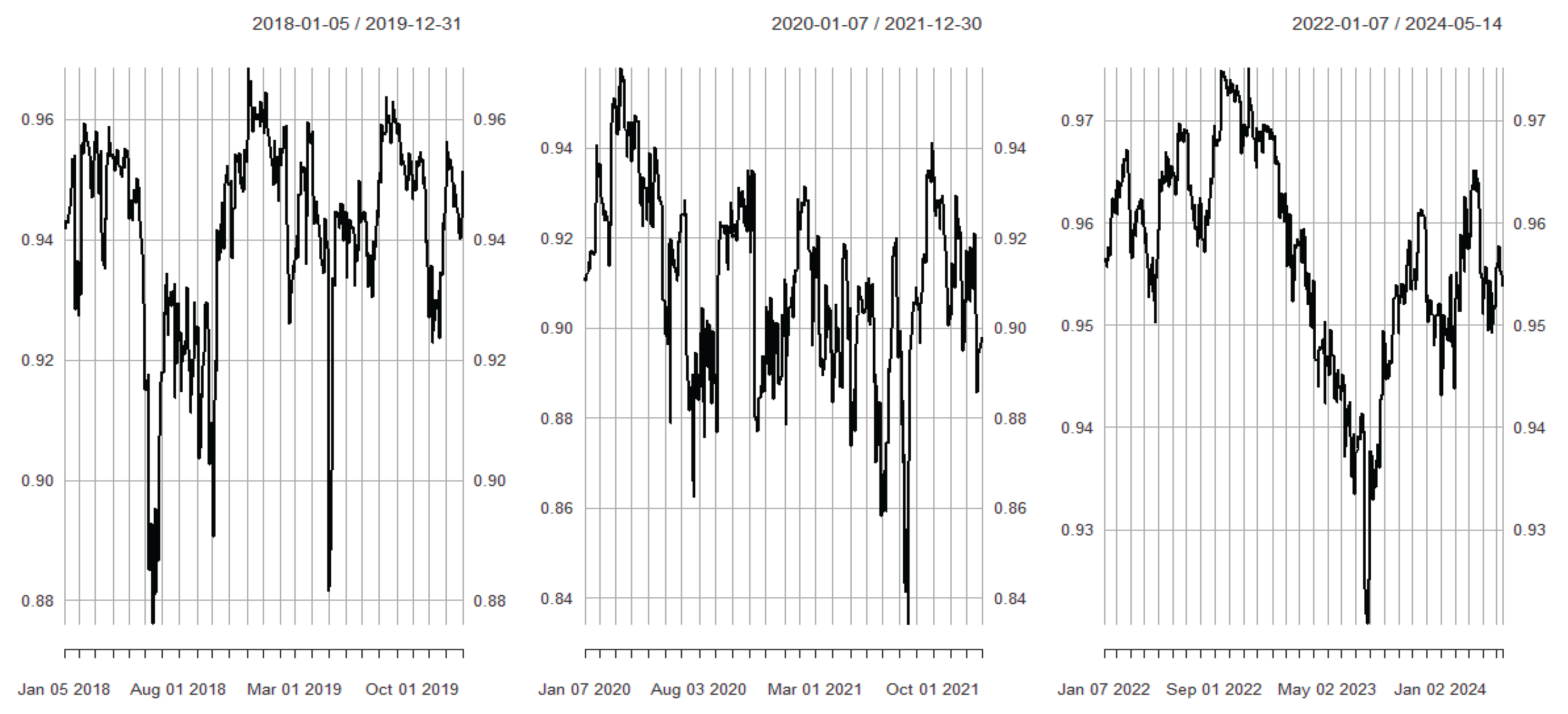
Figure 7.
Conditional correlation of Bitcoin with the SP500 over the 3 periods.
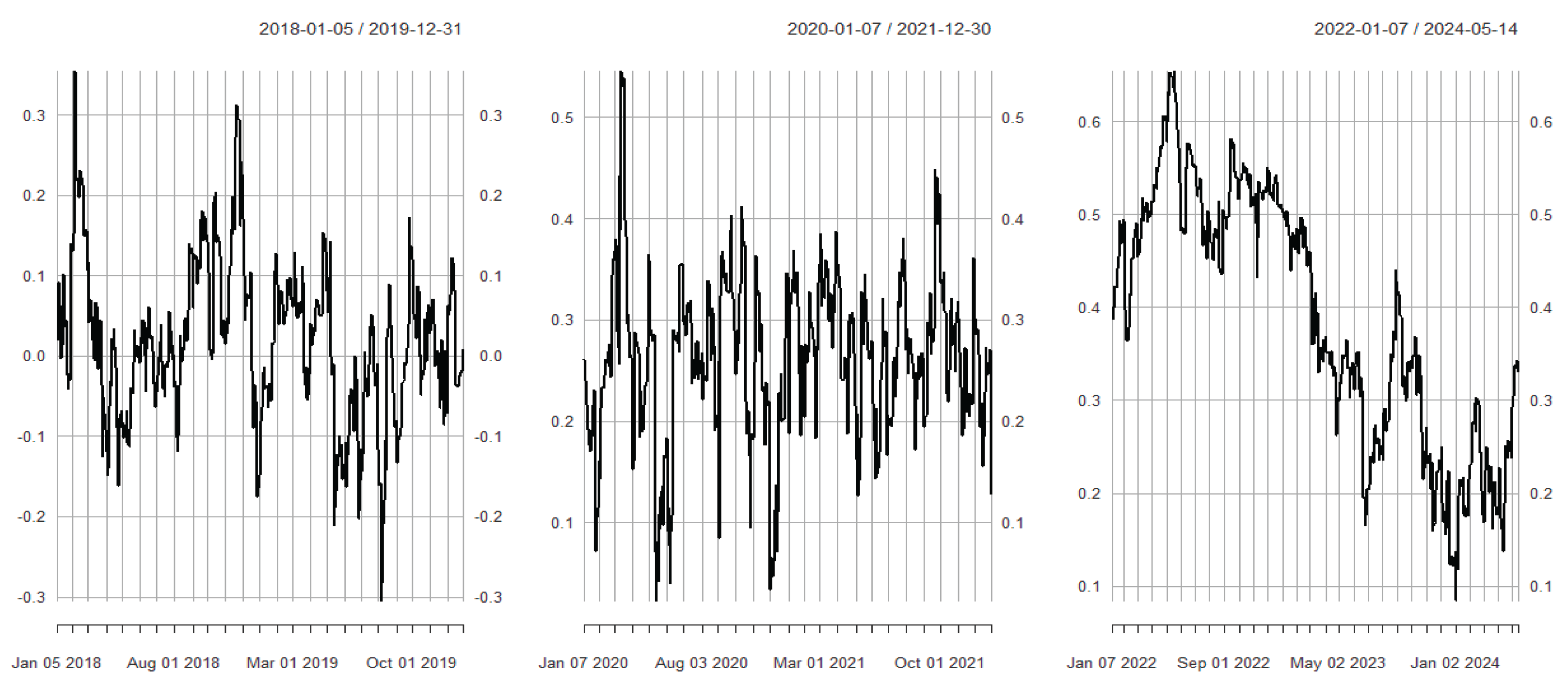
Figure 8.
Conditional correlation of the SP500 with the Gold over the 3 periods.
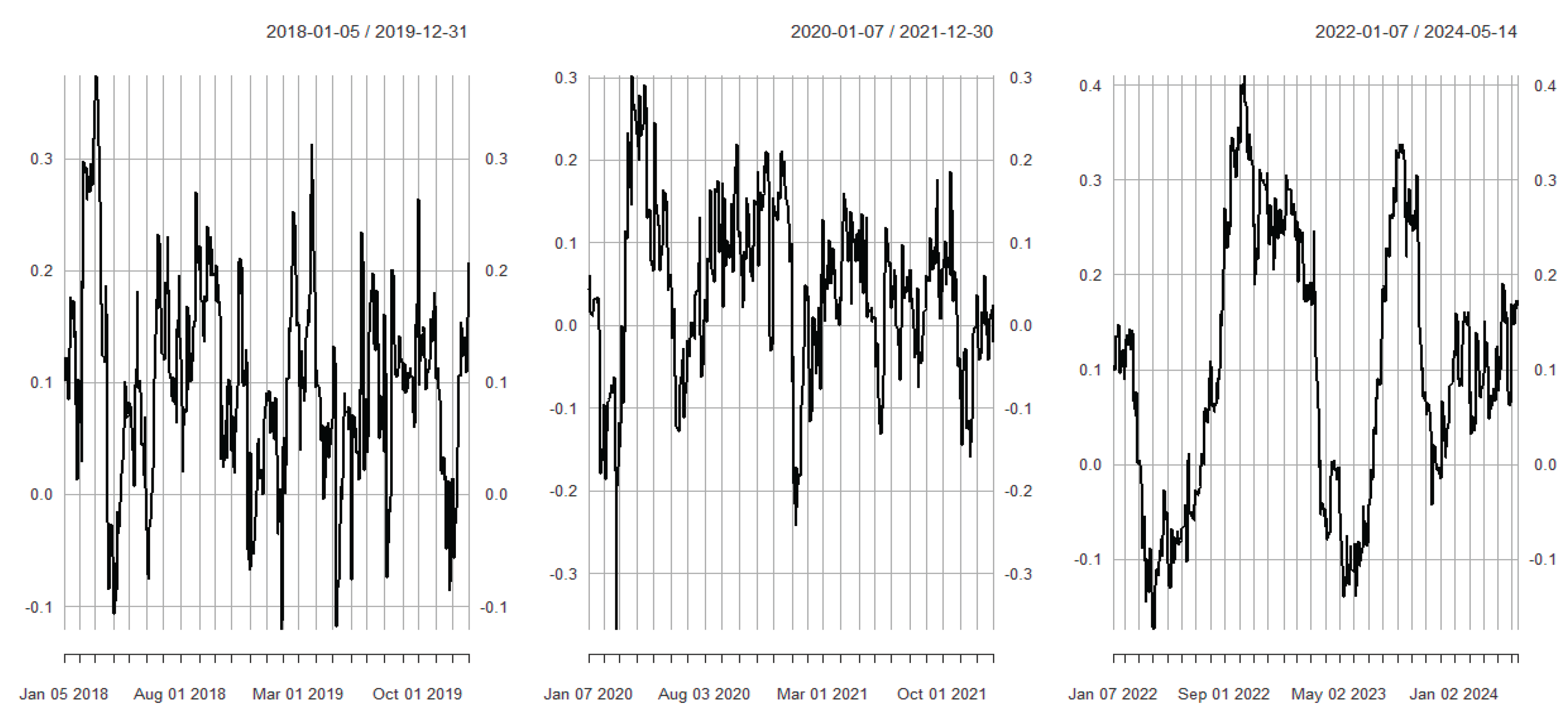
Figure 9.
Conditional correlation of Bitcoin with Gold over the 3 periods.
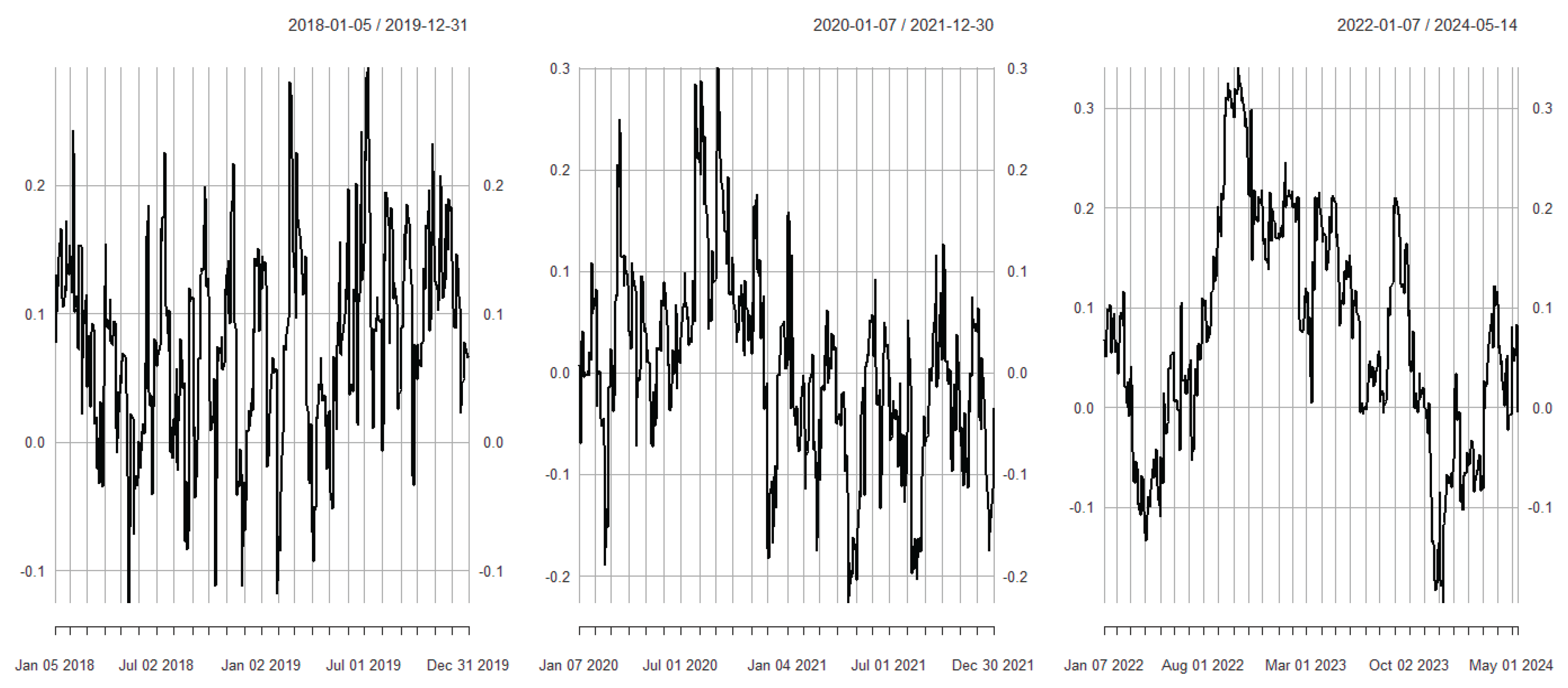
Table 1.
Descriptive statistics of the returns of the data (2018-2019).
| Statistics/Assets | GOLD | SP500 | DJIA | BITCOIN | NASDAQ |
| Minimum | -0.0247 | - 0.0418 | -0.0471 | -0.2410 | -0.0452 |
| Median | 0.0003 | 0.0009 | 0.0009 | 0.0008 | 0.0009 |
| Mean | 0.0003 | 0.0004 | 0.0003 | -0.0015 | 0.0005 |
| Maximum | 0.0288 | 0.0569 | 0.0600 | 0.2099 | 0.0606 |
| Std. deviation | 0.0068 | 0.0096 | 0.0099 | 0.0480 | 0.0118 |
| Skewness | 0.2306 | -0.4322 | -0.4172 | -0.2772 | -0.4093 |
| Kurtosis | 1.3717 | 4.5950 | 4.9556 | 3.1526 | 2.8936 |
Table 2.
Descriptive statistics of the returns of the data (2020-2021).
| Statistics/Assets | GOLD | SP500 | DJIA | BITCOIN | NASDAQ |
| Minimum | -0.05401 | -0.12765 | -0.13842 | -0.468625 | -0.13149 |
| Median | 0.0006 | 0.0018 | 0.0012 | 0.0031 | 0.0022 |
| Mean | 0.0004 | 0.0008 | 0.0005 | 0.0039 | 0.0011 |
| Maximum | 0.06790 | 0.08968 | 0.10764 | 0.1957 | 0.08935 |
| Std. deviation | 0.0106 | 0.0167 | 0.0176 | 0.0506 | 0.0181 |
| Skewness | -0.0152 | -1.0550 | -1.0451 | -1.6730 | -0.9848 |
| Kurtosis | 5.2813 | 14.4955 | 16.3914 | 15.8362 | 10.0142 |
Table 3.
Descriptive statistics of the returns of the data (2022-2024).
| Statistics/Assets | GOLD | SP500 | DJIA | BITCOIN | NASDAQ |
| Minimum | -0.0297 | -0.0442 | -0.0402 | -0.2634 | -0.0530 |
| Median | 0.0003 | 0.000 | 0.0003 | 0.0004 | 0.0003 |
| Mean | 0.0005 | 0.0002 | 0.0001 | 0.0005 | 0.0001 |
| Maximum | 0.0343 | 0.0540 | 0.0363 | 0.1810 | 0.0709 |
| Std. deviation | 0.0089 | 0.0118 | 0.0097 | 0.0372 | 0.0157 |
| Skewness | 0.0438 | -0.1759 | -0.1989 | -0.6215 | -0.1365 |
| Kurtosis | 1.1349 | 1.4775 | 1.5053 | 6.7903 | 0.9802 |
Table 4.
Connectedness table (2018-2019).
| GOLD | SP500 | DJIA | BITCOIN | NASDAQ | FROM2 | |
| GOLD | 95.61 | 1.18 | 1.88 | 0.81 | 0.52 | 4.39 |
| SP500 | 0.28 | 34.86 | 32.57 | 0.19 | 32.10 | 65.14 |
| DJIA | 0.44 | 34.06 | 36.50 | 0.10 | 28.90 | 63.50 |
| BITCOIN | 1.00 | 0.32 | 0.37 | 98.14 | 0.17 | 1.86 |
| NASDAQ | 0.15 | 33.85 | 29.05 | 0.17 | 36.68 | 63.32 |
| Contribution to others3 | 1.88 | 69.40 | 63.96 | 1.27 | 61.69 | 198.20 |
| Contribution Including Own | 97.49 | 104.26 | 100.47 | 99.42 | 98.36 | TCI4 |
| NET Spillover5 | -2.51 | 4.26 | 0.47 | -0.58 | -1.64 | 49.55 |
Table 5.
Connectedness table (2020-2021).
| GOLD | SP500 | DJIA | BITCOIN | NASDAQ | FROM | |
| GOLD | 85.61 | 4.22 | 3.76 | 1.68 | 4.73 | 14.39 |
| SP500 | 1.34 | 33.5 | 31.32 | 4.44 | 29.39 | 66.5 |
| DJIA | 1.33 | 33.67 | 35.24 | 4.08 | 25.68 | 64.76 |
| BITCOIN | 0.19 | 8.18 | 6.96 | 75.24 | 9.42 | 24.76 |
| NASDAQ | 1.38 | 31.84 | 26.12 | 5.22 | 35.44 | 64.56 |
| Contribution to others | 4.24 | 77.91 | 68.16 | 15.42 | 69.23 | 234.97 |
| Contribution Including Own | 89.85 | 111.42 | 103.4 | 90.66 | 104.67 | TCI |
| NET Spillover | -10.15 | 11.42 | 3.4 | -9.34 | 4.67 | 58.74 |
Table 6.
Connectedness table (2022-2024).
| GOLD | SP500 | DJIA | BITCOIN | NASDAQ | FROM | |
| GOLD | 93.47 | 1.92 | 1.66 | 1.22 | 1.72 | 6.53 |
| SP500 | 0.29 | 33.26 | 29.41 | 6.17 | 30.87 | 66.74 |
| DJIA | 0.34 | 32.12 | 36.32 | 5.56 | 25.65 | 63.68 |
| BITCOIN | 0.63 | 11.97 | 9.86 | 64.28 | 13.25 | 35.72 |
| NASDAQ | 0.19 | 32.63 | 24.81 | 7.22 | 35.15 | 64.85 |
| Contribution to others | 1.46 | 78.65 | 65.74 | 20.18 | 71.5 | 237.52 |
| Contribution Including Own | 94.93 | 111.9 | 102.06 | 84.46 | 106.65 | TCI |
| NET Spillover | -5.07 | 11.9 | 2.06 | -15.54 | 6.65 | 59.38 |
Table 7.
Tests on the standardized residuals of the VAR-NAR-NN models.
| Periods | LR test | ES test lag 1 | ES test lag 5 | ES test lag 10 | Conclusion |
| 2018-2019 | 0.000 | 0000 | 0.0050 | 0.002 | Evidence of time-varying correlation |
| 2020-2021 | 0.000 | 0.080 | 0.000 | 0.003 | In favor of time-varying correlation |
| 2022-2024 | 0.000 | 0.8401 | 0.051 | 0.001 | Less evidence of time-varying correlation |
Table 8.
Estimation of the WDDI index on the conditional correlation models.
| Residuals of models | WDDI index |
| Period: 2018-2019 CCC EGARCH (1,1) DCC EGARCH (1,1) |
0.126* 0.103** 0.116 0.094 |
| Period: 2020-2021 CCC EGARCH (1,1) DCC EGARCH (1,1) |
0.135 0.112 0.116 0.093 |
| Period:2022-2024 CCC EGARCH (1,1) DCC EGARCH (1,1) |
0.131 0.103 0.111 0.086 |
Orders *k=10, **k=5.
Table 12.
The mean conditional correlation of the DCC EGARCH model (for the period 2018-2019).
| GOLD | SP500 | DJIA | BITCOIN | NASDAQ | |
| GOLD | 1 | 0.0982 | 0.1141 | 0.0768 | 0.0715 |
| SP500 | 0.0982 | 1 | 0.9325 | 0.0185 | 0.9408 |
| DJIA | 0.1141 | 0.9325 | 1 | 0.0105 | 0.8175 |
| BITCOIN | 0.0768 | 0.0185 | 0.0105 | 1 | 0.0255 |
| NASDAQ | 0.0715 | 0.9408 | 0.8175 | 0.0255 | 1 |
Table 13.
The mean conditional correlation of the DCC EGARCH model (for the period 2020-2021).
| GOLD | SP500 | DJIA | BITCOIN | NASDAQ | |
| GOLD | 1 | 0.0420 | 0.0293 | 0.0061 | 0.0415 |
| SP500 | 0.0420 | 1 | 0.9320 | 0.2610 | 0.9101 |
| DJIA | 0.0293 | 0.9320 | 1 | 0.2336 | 0.7493 |
| BITCOIN | 0.0061 | 0.2610 | 0.2336 | 1 | 0.2902 |
| NASDAQ | 0.0415 | 0.9101 | 0.9101 | 0.2902 | 1 |
Table 14.
The mean conditional correlation of the DCC EGARCH model (for the period 2022-2024).
| GOLD | SP500 | DJIA | BITCOIN | NASDAQ | |
| GOLD | 1 | 0.1013 | 0.1115 | 0.0715 | 0.0695 |
| SP500 | 0.1013 | 1 | 0.9136 | 0.3852 | 0.9565 |
| DJIA | 0.1115 | 0.9136 | 1 | 0.3667 | 0.7907 |
| BITCOIN | 0.0715 | 0.3852 | 0.3667 | 1 | 0.3995 |
| NASDAQ | 0.0695 | 0.9565 | 0.7907 | 0.3995 | 1 |
Disclaimer/Publisher’s Note: The statements, opinions and data contained in all publications are solely those of the individual author(s) and contributor(s) and not of MDPI and/or the editor(s). MDPI and/or the editor(s) disclaim responsibility for any injury to people or property resulting from any ideas, methods, instructions or products referred to in the content. |
© 2026 by the authors. Licensee MDPI, Basel, Switzerland. This article is an open access article distributed under the terms and conditions of the Creative Commons Attribution (CC BY) license (http://creativecommons.org/licenses/by/4.0/).
Copyright: This open access article is published under a Creative Commons CC BY 4.0 license, which permit the free download, distribution, and reuse, provided that the author and preprint are cited in any reuse.


