

Submitted:
02 July 2026
Posted:
03 July 2026
You are already at the latest version
Abstract
A novel utility model of the daily electricity consumption patterns of any residential unit is proposed. The model is semi-parametric – its internal parameters are tractable to straightforward interpretations from the standpoints of microeconomics as well as game theory. The model considers two categories of appliances, fixed and shiftable loads. A modified Cobb-Douglas preference function is applied to incorporate utility tradeoffs in operating shiftable loads at different hours of the day, based on the consumer’s intrinsic preference and time-of-use pricing. The task of model parameter estimation is formulated in terms of constrained optimization, with an L2 error-based, regularized loss function, and ϵ-insensitive error constraints. It has been theoretically proven that there is a unique global optimum. A dual gradient ascent learning algorithm is developed to obtain model parameters that best fit real time series data of the unit’s daily shiftable and fixed loads. For a unit without sensors to separately monitor each load category, an unsupervised learning algorithm for partial load disaggregation is developed, which hybridizes the Gaussian mixture model with non-negative matrix factorization. Simulations with real data of two units highlight the effectiveness of the proposed methodology.
Keywords:
Cobb-Douglas preference
; convexity
; duality
; Gaussian mixture
; gradient ascent
; Lagrangian
; non-negative matrix factorization
; optimality conditions
; partial disaggregation
; unsupervised learning
; utility
1. Introduction
The overarching goal of this research is to develop a data-driven modeling framework of a residential unit’s daily electricity usage. A nonlinear model is proposed here that takes into account time-of-use (TOU) costs and ambient temperatures; it can be useful for a wide variety of tasks [1]. The model can be used by the consumer to detect excessive energy use times, predict monthly budget, in home energy management systems (HEMS), and modifying household activities. It can benefit architects and construction engineers in designing and retrofitting homes, and in the integration of renewable energy. Utility companies can adopt the proposed model to plan in advance installation capacity, analyze TOU pricing policies, improve preparedness for electrical outages, manage infrastructure costs, analyze demand response (DR), incentivize households’ electricity consumption in order to minimize grid stress, and to carry out large scale simulations of neighborhoods and towns for various energy market studies over large time periods.
Unlike a (fully) parametric model which relies on physical parameters of each electrical device (e.g., water heater, space heater, and clothes drier [2]), the model parameters do not reflect appliance level physics. At the same time, it differs from a non-parametric model whose parameters (however many) cannot be interpreted in any meaningful manner. Many such black box models have been proposed in current literature, based on deep neural networks (DNNs) and other machine learning methods (cf. [3]). Ergo, a semi-parametric model is proposed herein, whose parameters are firmly grounded in established econometric and game theoretic principles [4,5,6].
Two broad categories of household electric appliances are parametrized separately. These are, (i) fixed loads, and (ii) shiftable loads. In situations where these loads cannot be monitored separately, a novel algorithm for partial disaggregation of the aggregate load, has been proposed. This step can be used prior to parameter estimation of the utility model. Similar strategies, which do not disaggregate energy usage into individual appliance loads, have been adopted elsewhere [7,8,9,10,11].
Fixed loads are appliances such as lamps, LEDS, heating units, fans, stoves, ovens, refrigerators, freezers, and medical equipment, which can be operated at any time of the day, independently of the TOU cost. For instance, refrigerators and freezers must run throughout the day to prevent food spoilage, inevitably consuming electrical energy even during expensive peak periods. Likewise, lamps, LEDS, and fans are scheduled based on human occupancy and sunlight. Medical devices like CPAP machines or home dialysis units, must run according to patients’ health needs, regardless of TOU cost.
Shiftable loads are appliances such as EV charging, HVAC, and electric water heaters, whose energy usage is intermittent. These include high impact appliances that consume a large amount of energy that can be discretized into a few levels (e.g., OFF/ON or OFF/LO/MED/HI). Smart homes schedule these appliances according to the TOU cost of electricity. For instance, EV charging – often the largest single shiftable load, can be scheduled during overnight “super off-peak” periods, resulting in significant reduction in cost. While HVAC are required for comfort, “pre-cooling” or “pre-heating” a home before peak hours, allows the system to run less when rates are highest.
The schematic in Figure 1 shows how a typical load profile may change over time. Both classes of loads are shown. While fixed load appliances (top) are used throughout, shiftable load appliances (bottom) are operated intermittently. The figure also illustrates temperature dependent load variation. Detailed explanations are in the caption below.
In order to incorporate TOU dependence of shiftable loads, the proposed consumer model incorporates an extension of the Cobb-Douglas preference function [12,13]. The consumer’s preference for scheduling such an appliance in any hourly period of the day is regarded as a set of mutually competing tradeoffs. The log function is treated as the consumer’s utility [14,15,16]. In this manner, the latter is a saturating nonlinearity whose derivative is the unit cost of electricity [15,17].
A novel machine learning-based approach to train the consumer utility model, is proposed in this research. Using historical time-series data pertaining to residential energy consumption, ambient temperature, and local TOU policy, the model parameters can be adapted to reproduce a real consumer’s energy usage patterns during all 24-hourly periods of the day.
The overall scheme consists of one or two steps of unsupervised learning, depending on the availability of load data, (i) partial disaggregation, and (ii) parameter estimation. The latter step, which constitutes the core aspect of this research, is able to provide reliable estimates of the model parameters. It requires separate shiftable and fixed load data, which can directly be obtained from multiple sensors that monitor each load category. A purely non-intrusive alternative is to apply partial disaggregation to load data from single point sensor to monitor the aggregate load over time. In this manner, no prior knowledge of the appliances of a residential unit is assumed [9,18,19,20].
A novel hybrid algorithm has been developed for partial disaggregation. The fixed load component is extracted from the total (i.e., aggregate) load by expressing it as the weighted sum of independent basis vectors by means of Non-negative Matrix Factorization (NMF), an unsupervised learning algorithm that is used in many applications [21,22,23]. NMF uses multiplicative updates of the basis vectors and their weights, that can be revised as new load data arrives. The shiftable load component is represented as a Gaussian Mixture Model (GMM), which is extracted from the aggregated load data using the Expectation Maximization (EM) algorithm. The use of this algorithm in GMMs is a well-established method in machine learning [24,25]. The EM algorithm is flexible enough to allow changes in the GMM parameters’ update rules when new load data is used to replace or appended to the extant dataset. This step will be referred to as the Hybrid Unsupervised Partial Disaggregation Algorithm (HUPDA). To the best of the authors’ knowledge, HUPDA is the first effort to successfully hybridize EM-GMM with NMF as a standalone unsupervised learning algorithm.
The main step of this research involves training the parameters of the consumer utility model using the partially disaggregated load data that is either obtained directly from multi-point sensor monitoring or by means of the previous partial disaggregation step. The proposed consumer model’s parameters are trained so that its estimated hourly energy usage time series closely match the real time series. The difference between the two sequences is the error vector; its squared Euclidean norm serves as the quadratic objective function for minimization. A quadratic regularization term is added to the objective to ensure that there were no dramatic variations in the model parameters across two consecutive hourly periods. Linear inequality constraints ensure that relatively small discrepancies lying within a certain threshold are not penalized. In this manner, the overall problem has been formulated as a constrained quadratic program [26,29], which will be referred to as Semi-Parametric Unsupervised Model Algorithm (SPUMA) for the remainder of this article.
It is shown that there exists a unique global minimum of the underlying optimization problem in SPUMA. The Lagrangian dual is derived from the constrained optimality conditions, whence the training is carried out in an iterative manner [28,29]. Dual decomposition allows the parallel implementation of SPUMA as well as real-time updates as the residential unit’s load usage patterns slowly shift with time.
The overall mathematical framework is identical to that used to train Support Vector Machines (SVMs) for nonlinear regression [30], where estimation errors and model parameters are the primal variables (instead of the SVM’s weights). However, to the best of the authors’ knowledge, the literature on consumer parameter estimation in terms of a SPUMA in this manner, is sparse (if not non-existent).
1.1. Related Research
A comprehensive review of all significant residential consumer models has been published in [31]. In this article, the various modeling schemes have been divided into three basic categories, (i) bottom-up methods, (ii) top-down methods, and, (iii) hybrid methods. Bottom-up schemes use a different model for individual appliances. The appliance model parameters are referred to as micro-variables (e.g., thermal properties, load profiles, etc.). Hence, they are parametric models. These models are then grouped together into the household. The rate in such schemes may be as high as one sample per second. On the other hand, top-down methods represent entire homes as wholistic models [31]. The parameters of these models are referred to as macro-variables (e.g., aggregate loads, occupancy patterns, user preferences, etc.). Therefore, these are semi-parametric models that do not require appliance-level load profiles. These methods only need sampling rates that can be as low as once per hour. Hybrid modeling schemes are intermediate between bottom-up and top-down schemes. This research entails such an approach. It should be noted that non-parametric models are not considered in [31].
Only a limited number of studies have used fully parametric models of residential consumers in electrical grid applications. Such an approach has been proposed in [32] for a HEMS application. In a manner that bears a strong resemblance to this research, appliances have been categorized into curtailable and shiftable loads. A parametric model has been suggested for another HEMS application [33]. The trained model can be applied to schedule HVAC operation based on TOU price and automatically adjust smaller loads according to occupant comfort. Energy management in a community of residential units with solar panels and/or energy storage has been investigated in [34]. Consumer models of residential units are used to simulate their interactive behavior within the wholesale market. Only peak load specifications of home appliances have been used as model parameters. This is because this research is directed at long term planning applications, stretched over multiple years with seasonal changes. A parametric model for smart homes has been proposed in [35], to optimize energy consumption based on TOU pricing.
A variety of semi-parametric models have been investigated recently that render themselves to meaningful interpretation in terms of game theory, mechanism design, and/or machine learning. Fuzzy inferencing is used in a HEMS model for DR in [36]. Q-learning is applied to train the parameters. In the same manner as in this article, two categories of appliances are considered, shiftable loads and non-shiftable loads. In the approach taken in [37], multiple semi-parametric models based on consumer profiles are divided into clusters, in order to plan separate pricing policies for consumer clusters. Another HEMS model for DR applications has been suggested in [38] to obtain optimal thermostat settings of residential heating/cooling devices that minimizes cost. Relevant appliances are modeled separately. Since quadratic curve fits are used in place of physical parameters, they have been treated as semi-parametric models here. The approach in [4], is for aggregator day-ahead scheduling, and market planning applications, where modeling is based on prior consumer preferences to identify consumption patterns of different classes of industrial consumers. Prospect theory has been used to in [40] for semi-parametric consumer modeling. The approach incorporates psychological factors (i.e., risk seeking, risk neutral, and risk averse) into consumer models during variable energy pricing. The semi-parametric model in [41] uses Cobb-Douglas function along with perfect substitution, perfect complement to incorporate residential consumer’s preference tradeoff between energy consumption and battery storage. Different battery discharging rates have been studied in this study.
Machine learning algorithms such as NMF, GMMs, hidden Markov models (HMMs), and decision trees are included under the class of semi-parametric models as they offer some degree of visibility. A modeling method that hybridizes GMMs with Dempster-Shaffer theory has been investigated in [42]. It can be used to monitor unusual activity of patients in homecare facilities. The approach in [43] derives GMM parameters from multiple consumer usage time sequence patterns in buildings. A GMM based disaggregation method has also been used in [44]. An approach that uses a combination of K-means clustering and NMF to estimate consumer profiles has been proposed in [45]. NMF methods are used in [18,46] for load disaggregation. A matrix decomposition method similar to NMF is examined in [19]. HMMs are used to model individual appliances in [5] which preserves consumer privacy by means of a non-cooperative game theoretic framework. HMMs for load disaggregation have been extensively explored (cf. [8,20]). Decision trees and random forests have been used in [47] to model smart homes, which are trained using gradient boosting.
DNNs have been used to model consumers in [48], which takes into account the impact of weather in occupant comfort while minimizing HVAC load. Although DNNs are black boxes, the research makes use of the Shapley value, a cooperative game theoretic concept to garner meaningful explanations of DNNs; for this reason, the research has been labeled as an example of semi-parametric modeling in this article. A non-parametric residential model using Long Short-Term Memory (LSTM), which is a DNN has been proposed in [49]. DNNs are also applied in [50] for disaggregation, which are trained using federated learning. The article also provides a review of federated learning. For other detailed reviews of residential consumer modeling methods, the reader is referred to [1,2].
Concepts from algorithmic game theory have seen widespread use in the energy grid. Nash equilibrium is applied in [5] for a scheduling application. Prospect theory has been taken up in [6,40]. Mechanism design is used in bilevel energy trading in [14,15]. The double auction approach in [16] applies fairness to determine the unit energy costs that is charged to residential consumers. Disaggregated household consumption is applied for lower-level online bidding with the retailer in [51]. The bilevel approach is used to establish unit energy costs in a manner similar to [16]. Double auction energy trading algorithms have also been proposed in [14,15,16,52].
The Cobb Douglas preference function is routinely used in various application, such as wireless networks [53], governmental decision making [54,55,56], agriculture [57], economic risk assessment in energy systems [58], mining industry [59], community heating systems [60], renewable energy [61] and resource allocation [62,63]. It has also been adopted in energy grid research [41,64]. The Cobb Douglas function is very effective to represent tradeoffs, such as that between energy and spectral efficiency [53], renewable and non-renewable energy [55], capital and labor costs [59], repair and replacement [60], solar and wind energy [61], energy consumption and residential batteries [41] and energy consumption community-level storage [64]. A genetic algorithm is used to obtain suitable coefficients for the Cobb Douglas function [65], whereas the research reported here applies LICQP – a mathematically rigorous convex optimization method.
The utility of a consumer is quantified in econometrics as a saturating function of the quantity of resource consumed, with an asymptotic upper bound. For mathematical convenience, the logarithm function is widely used for this purpose, in various applications such as sensor networks [66], energy harvesting [67,68], surgical robotics [69] and energy systems [14,15,16,52,70,71]. Residential units equipped with solar panels and community level energy storage are modeled in [70]. The logarithm of the aggregate energy load serves as the consumer utility function. The derivative of the utility function is the unit energy cost of energy in trading applications [14,15,16,52,71].
Non-intrusive load disaggregation is a widely studied research topic nowadays. Several reviews and survey articles on the state-of-the-art methods have also been published. Many such reviews focus on HEMS for various applications, such as occupancy estimation, load forecasting, DR [72], appliance detection using simultaneous voltage and current sensor data [73], and their OFF/ON statuses in senior residences [74]. Reviews on disaggregation methods in HEMS and microgrids for various applications such as DR, assisted living, and anomaly detection [75], for DNN methods with sampling rates lower than 50-60 Hz [76], for e-monitoring techniques to encourage consumer participation in demand side management [77], and for fault diagnosis of HVAC appliances in buildings [78] have been published. Future research directions have been outlined in [79].
Since load disaggregation involves separating a single temporal sequence into its multiple constituents. Sans ample supplementary information, this is a very difficult task. Research proposals attempt to circumvent this difficulty in a variety of ways. Approaches in [45,46,80,81,82] apply supervised learning. Prior appliance profiles of all combinations of appliances are used with GMMs in [80] and HMMs [83]. The EM algorithm in [84] uses appliance level time series data to train HMMs. Pretrained HMM are used in [7]. The HMM approaches in [85,86] require prior appliance load profiles. Probabilistic methods are applied in [87] to analyze variation margins in trained machine learning models. Double Fourier spectra of voltage and current time series input data are used in [88]. Spectral graph theory is used in [89] to disaggregate energy usage in only a set of prior known appliances, while the remainder is treated as unknown appliance loads or noise. DNNs are perhaps the most widely used models for disaggregation. Convolutional neural networks (CNNs) are used in [51,88,91,92]. Temporal processing is handled by incorporating LSTM and/or biLSTM blocks within the DNNs in [51,92], as well as by attention mechanism and transformer blocks in [91,93,94,95]. A relational network is used in [96], and a generative adversarial network (GAN), in [97]. A novel pyramidal structured DNN is proposed in [98]. Since DNNs depend on supervised learning, to maintain consumer privacy, current research methods use transfer learning [8,96,99], and federated learning [11,95,98,100,101]. Clustering algorithms are sometimes applied to group together similar appliances in [83,102], or multiple home units [11]. The disaggregation method in [103] exploits strongly correlated PV generation of buildings in a neighborhood. Many approaches detect and/or use switching events of appliances for disaggregation [94,96,104]. Synthetic training data have been used in [10,93,97]. A very limited amount of research do not require prior disaggregated data, pre-trained models, appliance characteristics, simultaneous voltage and current measurements, occupancy information, or correlated usage (cf. [5,9,18,42]). Since single-point monitoring is the only requirement, these methods can be adopted universally.
Problems formulated as linear and quadratic programs have been used in energy grid applications. A mixed integer linear programming problem in [10] is handled using an algorithm that hybridizes branch & bound with genetic search. Disaggregation methods involving quadratic programming have been investigated in [7,84,89]. An algorithm that hybridizes sequential quadratic programming (SQL) with a genetic algorithm has been explored in [105] for a microgrid protection application. SQL has also been considered in [106] for a market-oriented scheduling problem, and in [107] for use in an electric vehicle problem and in [108] for economic dispatch. Karush-Kuhn-Tucker (KKT) conditions for optimality have been explicitly applied in [109] for another economic dispatch problem. The performance of SQL has been compared with swarm intelligence and other metaheuristics in [106,107,108].
1.2. Research Contributions
The significant contributions of this research are along the following main directions, (i) a semi-parametric model of the daily electricity consumption within a residential unit, (ii) a data-driven parameter estimation algorithm that finds rigorous theoretical support, (iii) an unsupervised, hybrid learning algorithm for categorical disaggregation of loads; moreover, the above discussion and extensive references show that this article provides (iv) a concise, state-of-the-art review of recently published research in all relevant topics. These directions have been further elaborated, each dealt individually below.
- Semi-Parametric Model
The semi-parametric model aims to fill a crucial gap in current large-scale simulation-oriented research, which tend to represent energy consuming units with ad hoc models [4,14,15,16,36,37,38,40,52]. This is the case with the macro-variables used within semi-parametric energy consumer models that apply fuzzy logic or Dempster-Shaffer theory; moreover, their interpretabilities are domain-specific in nature. General purpose, game-theoretic models, which can be used in energy market research, are sparse in the existing literature. The methodology proposed herein attempts to address these limitations.
There are other desirable features in this article’s approach. It can be extended to include other influencing factors, such as the occupancy rates at different periods in a day, and the home consumer’s own environmental awareness. It is also upwardly scalable to buildings, offices, apartment complexes, neighborhoods, and even cities; if necessary to avoid computational overloads, the model can be simplified by considering larger time periods, reducing the load sampling rate, scalarizing the model’s vector parameters, or excluding cost and/or temperature data.
- Parameter Estimation Algorithm
SPUMA – the proposed estimation algorithm is of equal significance. Metaheuristics, that are often used in similar research work [65,105,106,107,108] are associated with unavoidable shortcomings. Due to their randomness, multiple runs are needed in order to determine statistically significant performance metrics. Unlike gradient ascent, they use populations of candidate model parameters that not only place unnecessary computation overheads, but also make them slower to re-adapt to shifting electricity usage patterns. In contrast, the proposed algorithm is wholly deterministic, with guaranteed performance metrics.
It will be shown in the next section that the algorithm, being a dual decomposition method, can be readily parallelizable. As a gradient ascent approach, its computational requirements are minimal in nature. Lastly, all aspects of SPUMA are well grounded in convex optimization theory. Despite its close resemblance to iterative training in SVMs, significant differences do exist in how regularization function as well as the inequality constraints have been formulated. These have been provided in the following section, with derivations postponed until the appendix.
- Partial Disaggregation
The article introduces HUPDA as a new algorithm to disaggregate the overall energy load into two broad categories. It represents one of the few algorithms that have successfully hybridized NMF and GMM. Unlike many other non-intrusive load monitoring (NILM) approaches [10,80,83,93,97], this algorithm does not need any prior knowledge of installed appliances, multiple sensors, switching event detection, or model pre-training. It requires uniformly sampled aggregate load data, which can be obtained directly from non-intrusive, single-point monitoring alone.
- Literature Survey
The previous subsection of this article provides a summary of current research in the all topics closely related to this research with appropriate references. It could be of benefit to the energy grid community as a brief review of recent research advances.
2. Materials and Methods
The symbol represents the ordered sets of time instants covering an entire day. Likewise, is the ordered set of samples, where each sample pertains to a full day. At time instant in sample day , the aggregate, shiftable, and fixed loads are , , and . As they must be non-negative quantities, , and,
The quantity in the above expression is a zero mean, iid random variable representing noise, so that and . Since HUPDA and SPUMA have in-built error components that subsume noise, the third term in the above expression can be ignored.
For the sake of conciseness, the following convention is adopted hereafter. Suppose is some ordered set of indices, such that there exists a scalar for each . The vector whose th element is is, which is of size . The same vector may be represented in a more convenient manner as shown,
Next, suppose that there exist vectors for all , of equal size, . The vectors can be arranged as the columns of a block matrix , which is of size . Our convention allows to be expressed more concisely as,
Another way to express the same matrix whose rows are in and columns in is,
This convention, allows us to define three vectors , that represent sequences of aggregate, shiftable, and fixed energy usage during any day (or sample) . In the manner of Equation (2), the vectors are,
The unit cost of electricity remains fixed throughout a period; based on the TOU, any change can only take place only at the first instant of any period. Furthermore, the temperature data is recorded only once per period. Therefore, for compatibility, the instants in are grouped into contiguous, non-overlapping periods of equal duration. If is the ordered set of periods, then must divide . For example, if the load is sampled once every min, and each period is an hour, then for a day, mins, and hours, so that mins. Therefore, for some ,
It can be readily seen that the th period () of the day must begin at time instant, , and end at another instant, . Associated with the same period is a binary vector, and its th element () is . This indicator vector is given as,
The quantity represents the vector of all ones (i.e., . Clearly, the tensor product is a binary vector of size , which is the also the size of any load vector defined earlier in Equation (5). All but elements in this tensor product are zeros. The elements between the positions and are ones. It follows that the inner product of with a daily load vector is the corresponding net load used during period . The net aggregate, shiftable, and fixed loads used during period of any given day can now be defined,
The corresponding load vectors, covering all periods in for the same sample , are given as,
Temperatures have been recorded periodically each day. The recorded temperature for sample during period is , and the corresponding temperature vector is,
Based on TOU pricing, the unit cost of electricity for period is , which does not change with day. The vector of daily unit costs, denoted is given as,
The load vectors defined in Equation (5) can be arranged as the columns of the load profile matrices, as shown below,
In the same manner, three periodic load profile matrices, can be constructed in this manner,
2.1. Utility
The resources complement one another when a consumer’s requirements can be met by using both. For instance, a left and a right shoe are complementary resources so long as they have the same color. Suppose a person owns three left shoes (red, green, blue) but two right shoes (red, green). Effectively, it (To remove potential bias, the neuter form of the third person pronoun is used throughout this article.) has only two pairs of shoes to choose from. Conversely, two resources can supplement each other. For example, a person gains equally by consuming either 12 oz. Coke, 12 oz. Pepsi, or 7 oz. Coke and 5 oz. Pepsi. Unlike shoes, drinks are divisible resources. A person who prefers Pepsi over Coke, may gain equally by consuming either 12 oz. Coke, or 10 oz. Pepsi, or 6 oz. Coke and 5 oz. Pepsi. Resource divisibility allows the use of coefficients to quantify relative benefits derived from using resources; in the last example they may be in the 5:6 ratio.
Next, let us examine a more generic situation with two resources. Let be the amounts consumed by a certain consumer. The overall gain that it derives from their combined use is some non-decreasing function, say . When the two resources exhibit perfect complementarity, the consumer’s gain is , where are two coefficients intrinsic to the consumer. On the other hand, when the resources display perfect substitutability, then its net gain .
The Cobb-Douglas function is to represent the intermediate situation where the resources are neither complements nor substitutes of one another. The consumer’s net gain can be expressed as . The schematic in Figure 2 shows the shape of a typical isoquant for the Cobb-Douglas function. For comparison, isoquants for perfect substitution and perfect complement, are also shown in Figure 2.
In general, with representing the vector of all resources, the Cobb-Douglas preference, with multiple resources indexed , consumed in amounts is,
The parameters are referred to as elasticity constants that sum up to one.
The consumer’s utility from using , is its logarithm, . Using the logarithm offers a threefold advantage, for it makes the utility: (i) non-decreasing, (ii) strictly concave, and, (iii) Lipschitz continuous. Together, these advantageous features ensure that the shape of the utility function is in conformity with the law of diminishing returns. Based on the above rational, if is the shiftable load used by a residential unit, its occupants’ utility must be , where and are model parameters for the period that do not vary with day . The function is equal to the natural logarithm of its enclosed argument, but lower bounded at zero. The parameter is the base component of the shiftable load for period , which is governed by extraneous factors (e.g., it is not practical to operate a washer/dryer unit at 2:45 AM). The parameters and are two constants of proportionality such that is a temperature-dependent baseline. In general, the energy consumption increases when the ambient temperature deviates in either direction from an occupant-specific optimum (that maximizes its comfort). Under these circumstances, the absolute difference between the real temperature and (i.e., ) should have been incorporated in the argument of the function . However, as the specific data sets used in this study involve only warmer, summer days, it may be conveniently assumed that . Thus, the expression for the utility function is,
Figure 3 illustrates how the utility function (top) and its derivative (bottom) vary with shiftable load. Note that the function’s derivative is also the cost per unit of energy. The figure also shown the fixed load.
2.2. Estimation
The derivative of the utility function in Equation (15) with respect to is the marginal utility, which is also the unit cost , so that . A few algebraic steps lead to the following model-based approximation of the shiftable load,
The above equation splits the shiftable load into cost dependent, constant, and temperature dependent terms. The ‘hat’ () over any load variable indicates that the resultant is an estimate of . Thus, is an estimate of the true load .
Fixed loads pertain to appliances such as lighting and refrigeration, which are typically operated continuously and independent of the unit energy cost. It is assumed that the net fixed load at any period consists of a constant term and a temperature-dependent term. Using and as two other model parameters, the estimated fixed load is given by,
2.3. Hybrid Unsupervised Partial Disaggregation Algorithm
The total shiftable load at instant in day follows a GMM distribution. The probability that is the sum of Gaussian terms as shown below,
where is defined as per the Gaussian distribution,
The mean of the th Gaussian is (), where is the set of non-zero mean Gaussians in the GMM and when no shiftable appliance is in use. Figure 4 shows an example of such a GMM with six Gaussians (i.e., ). All Gaussians share the same width parameter , a small, positive constant () that accounts for random noise. Only a single Gaussian, may be active at any instant . The parameter is the prior probability of the th Gaussian.
The mean of a Gaussian can be equated to the load usage (in kW) of any shiftable appliance. However, as the total number of shiftable appliances present in the household is not known a priori. To address this lack of information, must also represent the overall load when combinations of two or more appliances are operated simultaneously; the cardinality must be high enough to cover all cases. The caption placed immediately below Figure 4 provides further insights that are specific to the GMM example shown in the figure.
Based on NMF, the fixed load vector, of each sample day , is represented through of a set of basis profiles, (), that are non-negative and orthonormal vectors (i.e., , where is the Kronecker delta– ). Each basis vector has its weight , and the fixed load , is their weighted sum,
It may be observed that all sample days are represented through the same set of basis vectors, but weighted differently with day. This is because each basis reflects a specific pattern, whereas actual load profiles are not identical every day . To further explain this rationale, let us consider a simple scenario where a residential unit’s fixed load consists of lighting equipment and a freezer. Since lighting is used only during evenings, HUPDA may train itself to incorporate this pattern as a basis vector in . On the other hand, while the freezer’s load directly varies with daily temperature. HUPDA may select one basis vector (“warm”) to model a sunny day in the dataset, and another basis (“cool”) for a day that was overcast at all times. Whereupon, a day that is sunny during the morning periods, and overcast thereafter, may be apply higher weights to the “warm” basis until noon, slowly transitioning to instants where the “cool” basis is weighed more.
The basis vectors make up the columns of a basis matrix, ,
A weight matrix can be constructed whose elements are the weights () as follows,
Figure 4 illustrates how the columns of the fixed load matrix are captured by NMF with the matrices and ; as per Equation (20). The caption appearing beneath the figure elucidates this representation. An estimate of the fixed load profile matrix is computed in this manner, whence,
The trainable parameters are the Gaussian priors (), and means (), as well as the NMF’s basis and weight matrices, and . These parameters are incremented using and , which are the GMM and NMF learning rates respectively. It must be noted that all these quantities are meant for internal use within HUPDA, whose purpose is to deliver estimates of the load matrices, and from their aggregate .
Although the sequential order of time instants in is preserved throughout the learning process, the samples in are randomly rearranged at the onset of an iteration. An iteration hitherto will refer to a single loop through all sample days .
The EM algorithm involves latent variables which are posterior probabilities; more specifically, During the E-step (estimation), the posteriors are approximated in two steps in the manner shown next,
Equation (24) merely obtains the variables , which is the denominator in the RHS of Equation (25) to normalize so that .
The prior probabilities are incremented as shown below,
As the Gaussians are directly linked with the overall load when some combination of (zero, one, or more) shiftable appliances are in use at the same time, their prior probabilities at different time instants should be different. However, it can be seen that the prior does not have as subscript. This is because the increment in Equation (26) is applied in their proper order in , so that at any instant , in the RHS of Equation (26) is the prior from the previous instant, . As long as is strictly meant for internal use inside HUPDA, incrementing it in this manner ensures that there are no abrupt changes between two consecutive instants.
The Gaussian means are incremented in a similar manner,
The shiftable load can be estimated in the following manner,
The estimated shiftable load matrix is removed from the aggregate load matrix to provide the estimated fixed load matrix that is used to update the NMF matrices,
NMF attempts to decompose into matrices and , and there are several NMF algorithms that can accomplish this task. The NMF used in this research iteratively converges towards optimal values of and at the minimum of the Frobenius norm of the difference, , while preserving the orthonormality of , as well as the non-negativities of and ,
Everywhere in this article, is the identity matrix. The basis and weight matrices from the previous iteration of HUPDA are incremented next. The weight matrix is incremented in the following manner,
In the above, is the Hadamard product of and , and is their element-wise inversion of ; so that if the element in row , column of is , then the element in the same row and column of is . In this manner if , , are matrices of the same size, then so would be , and any other Hadamard product formed from them.
To preserve orthonormality, the basis matrix is incremented in a somewhat different manner as follows,
2.4. Semi-Parametric Unsupervised Model Algorithm
Since unit costs and temperatures are recorded once per period, SPUMA uses a somewhat coarsely grained load data. Its inputs are the shiftable and fixed load matrices , which are transformed into the corresponding periodic matrices as in Equation (8). Although all noteworthy aspects of the algorithm have been explained here, for the full derivations of some of the equations, the reader is referred to the Appendix.
As a convenient reminder, are two vectors of all ones and zeros, is an identity matrix, and is an matrix of all zero elements. All of the above quantities are used throughout this article, with subscripts indicating size.
2.4.1. Constraints
SPUMA uses two algorithmic constants and , that establish tolerance bounds. Smaller errors that are within these bounds are not penalized; this is how errors are typically handled in SVM regression.
The quantities and in Equation (16) are shiftable load model parameters at period , whose optimal values are to be determined by SPUMA. In the same manner as in Equation (9) and Equation (10), let the vectors be defined as,
Given any sample , let us consider the shiftable load consumed at . The LHS of Equation (16) is the estimated load, . The RHS of Equation (16) is the model-based approximation of the same load. The difference between them should be within established bounds, i.e., . Any excess difference is an error that incurs a penalty. With the vector of such errors being represented as , the inequality constraints for all periods in of the sample day , can be expressed as,
Referring to Equation (16), it is evident that the fixed load must be bounded on both sides as, . Before introducing the analogous, vectorized constraints for the fixed load, let us define the parameter vectors ,
The inequality constraints for the fixed load vector can be expressed in terms of the error vector . in the same manner as in Equation (36), as follows,
2.4.2. Error & Regularization
An error within any period in can only occur if there is a bound violation; the corresponding scalar element in or may be either positive or negative. To prevent cancellations, error functions in SVMs and elsewhere use normed error terms. Specifically, the weighted sum of the squared Euclidean error norms and are adopted in SPUMA. With as weights, the error function , is given as,
The parameters of the semi-parametric model are . Since they are vectors of the same size, let be a representative parameter vector, which may be any of . At two consecutive periods , the components and , must not be significantly different. Putting it in another way, it is desired to keep their squared difference low. This can be accomplished by adding regularization terms for the model parameters. These terms will be formulated using the shift matrix , whose columns have been defined earlier in Equation (7),
The subscript in Equation (41) is a unit increment of index , modulo . For , , but . The product , so that is the sum of terms of the form . Regularization terms of this form are used in SPUMA. Let be the following matrix,
A few algebraic steps will show that . The regularization function is formulated as shown in the following expression,
2.4.3. Problem Formulation
The primal variables in the optimization framework are the error vectors and the model parameter vectors . For brevity, the error vectors are consolidated into the following single vector ,
From Equations (16) and (17), it can be seen that are the coefficients of temperature independent terms, while are those of temperature dependent terms, they are incorporated into two vectors, and , which are,
Before presenting a concise framework of the same optimization problem, the matrices , which will be incorporated into the objective function are as below,
Using Equations (41) and (43) and the above definitions, the loss function can be expressed simply as .
A similar approach is used in SPUMA, its constraints expressed in terms of three matrices , and a vector that are introduced next,
Using the above quantities, the constraints in Equations (36), (39) can be expressed in a compact manner as .
The constrained optimization problem can be formulated with the loss function as the mapping , and the linear constraint function as another mapping . The constrained optimization problem in SPUMA is presented in a formal manner below.
Minimize (w.r.t. ):
Subject to:
Appendix A.1 and A.2 show detailed derivations of the above expressions for the loss and constraint functions, which are also Equation (A1) and Equation (A2).
Theorem 1.
In SPUMA: (i) The loss , is strictly convex with respect to; (ii) The feasible region given as is a convex polytope; (iii) There is a unique global minimum.
Proof. The matrix in Equation (47) is obtained as the tensor product of with an identity matrix. Both factors in the product are symmetric matrices. Moreover, since the weights , are strictly positive quantities, and is positive definite, their tensor product must be a symmetric, positive definite matrix,
The shift matrix in Equation (42) is a permutation matrix that has one and only one element in each row and in each column that is one; its remaining elements are zeros.
Let be an arbitrary vector. The squared L2 norm of the difference between the original and shifted vectors is,
Replacing with in the RHS and expanding it yields,
Separating the factors and in each term in the RHS,
From Equation (41), it can be seen that the second factor () in the RHS of the above equality is the matrix . Replacing it with the latter,
Since the squared Euclidean norm in the LHS is necessarily positive, it is evident from the above equality that the RHS for any vector . In addition, it can be seen that since are symmetric matrices, so is . This shows that is a symmetric, positive definite matrix,
The matrix defined in Equation (48) is the tensor product of the diagonal matrix , and , both of which are symmetric, positive definite. As the tensor product of two symmetric, positive definite matrices must also be symmetric, positive definite, it follows that,
The same rationale can be used with Equation (49) to establish that,
The Hessians of shown in Equation (54) with respect to its arguments are,
As the loss function’s Hessian with respect to and are symmetric, positive definite matrices, the function is strictly convex. This establishes statement (i).
From Equation (55), the inequality constraint is,
Each row of the above expression is a hyperplane in . There are such hyperplanes. It follows that their intersection is a convex polytope (not necessarily bounded). This establishes statement (ii).
A strictly convex function with a convex feasible domain must have a unique global minimum, it follows that the constrained optimization problem in SPUMA also has a unique global minimum. This establishes statement (iii).
All three statements, (i), (ii) and (iii) of this theorem have been established above. This concludes the proof of Theorem 1. □
Theorem 1 shows that starting from an arbitrary initial point, iteratively updating the variables and along the gradient direction would lead to steady convergence towards the optimum . Unlike the other methods discussed earlier, stochastic methods or metaheuristics are not needed. This is the underlying justification for using dual gradient ascent to obtain the optimal model parameters in SPUMA.
2.4.4. Dual Decomposition
For each sample , there exists the corresponding inequality constraint of the form, . Let its dual variable be , so that . Applying the KKT first order stationary conditions to the problem yields , expressed in terms of the aggregate variables, , which are given as,
These expressions appear in Appendix A.3 as Equations (A3-A5).
The stationary conditions are applied to yield the following optimal primal vectors,
These expressions are identical to Equations (A6-A8) in Appendix A.3.
The gradient update rule for the dual variables , whose derivation is again relegated to Appendix A.4, is,
This is Equation (A9) in Appendix A4, where is the gradient step size.
2.4.5. Dual Gradient Ascent
Equations (56)–(58) are used in each iteration of SPUMA to update values of using the previous values of , whereupon Equations (59)–(61) are applied to determine the new values of . The dual is initialized to zeroes and subject to iterative increments as per Equation (62). The algorithm terminates when the inequality constraint in Equation (55) is satisfied. In order to keep track of the termination condition, a Boolean variable () is maintained internally in the algorithm.
The steps of the algorithm are outlined in Figure 5. In the flowchart it is assumed that in the loss function, have been precomputed in accordance with Equations (47)–(49), that and in the constraint bound have also been determined a priori through Equations (50)–(53); furthermore that they are directly accessible to the iterative parameter estimation algorithm.
The schematics in Figure 6 illustrate the steps of the proposed approach,
3. Results
The simulation results reported here used actual energy usage data pertaining to two residential customers, User-1 and User-2, which was obtained from the Pecan Street Inc., Dataport database [110] sampled at the rate of once per minute, and for a total of 61 days during the months of March and April of 2018. The database included individual appliance usage measurements at the circuit level. The following are the main appliances, (i) air condition, (ii) electric car, (iii) washer/dryer, (iv) dishwasher, (v) microwave, (vi) refrigerator, (vii) furnace, (viii) bedroom apps, (ix) light plugs, and (x) kitchen apps. The first five appliances are classified as shiftable loads, and the remainder as fixed loads. It may be noted that some of these appliances were not common to User-1 and User-2. User-1 did not use bedroom apps and furnace, while User-2 did not own an electric car. The shiftable and fixed loads were stored as arrays, separately for User-1 and User-2. In this manner, two raw datasets were obtained, each consisting of sample vectors, , where .
The hourly temperature data for same 61 days was also obtained from [110]. The hourly time of use rates were obtained from the Austin Energy website [111]. The website provides electricity rates in the Austin area for a time of use pilot project. The user data used in this study were part of DER that received pricing information from the utility and were expected to defer their loads during peak or high energy price hours.
Prior to applying SPUMA, the raw load datasets of User-1 and User-2 as well as the temperature data were further divided into two sets – one for Month-1 (March), and the other for Month-2 (April). There were samples in Month-1, and in Month-2. Since the unit cost time sequence is the same in all samples, it was not changed.
A total of four datasets were obtained in this manner, uniquely identifiable from the user label (i.e., User-1 or User-2) and the month label (i.e., Month-1 or Month-2). Each dataset contained the load matrices , hourly temperatures of each daily sample and hourly unit cost , where . The periodic load matrices were computed as provided in Equation (13).
All simulations reported in this section used the MATLAB® software package and the constrained optimization toolbox (fmincon() built-in function). Table 1 shows the values of various algorithmic constants in Equations (36,40,43). The weights of the parameters were assigned relatively small values in order to increase their sensitivities to variations in the daily unit costs and temperatures. The constraint bounds were the sum of a constant baseline and a suitably scaled load norm; denotes the Frobenius norm of matrix in Table 1.
The two plots in Figure 7 depicting the learning algorithm’s steady convergence towards the unique, global optima for each dataset. The log Lagrangian dual function and the log maximum constraint violation are plotted against the log iteration. In all four cases the algorithm terminated when the constraints were tightly bounded. The y-coordinates in both plots are raw values that have not been normalized w.r.t. dataset sample size or the algorithmic constants in Table 1.
Table 2 contains the outcome after termination of the algorithm. The error vectors are incorporated in the bound constraints in Equations (36) and (39). The two terms in the quadratic loss are the error function and the regularizing function in Equations (40) and (43). The total computer time taken to converge is also shown.
Figure 8 shows the values of the parameters in the shiftable load and of the fixed load in the semi-parametric consumer model for each period in . Each parameter is shown separately, as a plot of its numerical value vs. period .
Figure 9 and Figure 10 show scatter plots. The x-coordinates of each point are the model parameters obtained using SPUMA with partially disaggregated real load matrices as inputs. The y-coordinates were obtained after HUPDA was used for partial disaggregation which were used by SPUMA to estimate the same parameters. The scatter plots in Figure 9 are model parameters and of the shiftable loads, whereas those in Figure 10 are and of the fixed loads.
Figure 11 and Figure 12 illustrate how the proposed semi-parametric model can be leveraged to generate the consumers’ electricity usage profiles on typical days. They shaded regions show the ranges of distributions of the raw loads in the datasets. The shiftable load consumption patterns in Figure 11 were obtained as . Those of the fixed loads shown in Figure 12 were obtained as . The four datasets are plotted separately in both figures.
4. Discussion
The steady convergence of the iterative dual decomposition algorithm can be readily observed from the plots in Figure 7. Conservative dual increments per iteration successfully avoided overshooting. Only 100 iterations were sufficient to ensure that the optimization algorithm had been attained while using each of the four datasets.
Table 1 provides a summary of the results of the optimization process in SPUMA. The raw loss components and in Table 1 quite high as is the sum of quadratic terms and pertain to 21 or 22 days. Additionally, the raw values are lower for User-1 than for User-2. The same pattern is seen after scaling with respect to the weights. While refraining from providing concrete reasons, it is possible that the energy consumption profile of User-1 is more routine than that of User-2. An alternative artifact may lie in the nature of the appliances installed in the home units of User-1 and User-2. It should be noted that the computing time taken by the built-in function (fmincon) in MATLAB® in this table are when the dual variables were sequentially updated. Running SPUMA on a hardware that supports parallel processing would improve the speed.
Figure 8 shows how the model parameters, , for the shiftable load, and , for the fixed load, estimated separately for each dataset and for each hour of the day. The effect of regularizing the loss function in SPUMA was to ‘flatten’ them, so that they did not rise or fall too sharply across hourly periods. It can be observed that the shiftable load parameters for User-2 follow very similar hourly trends in spite of different scales (specifically the green lines). Since is sensitive to the unit cost () while is a baseline component for hour , it is hypothesized that User-2 is less cost conscious compared to User-1. More experimentation may provide further insights. The weights assigned to the regularization terms may always be adjusted to produce the most desirable outcomes depending on the application.
The scatter plots in Figure 9 are those of the consumer model’s shiftable load parameters and . In all four datasets, it can be seen that the absence of separate sequences for each load category did not produce dissimilar parameter estimates, indicating the effectiveness of HUPDA to preprocess aggregate load prior to SPUMA.
It can be seen that the scatter plots in Figure 10, which are those of , , show very similar parameter correlations.
Abbreviations
The following abbreviations are used in this manuscript:
| TOU | Time-of-Use |
| HEMS | Home Energy Management System |
| DR | Demand Response |
| DNN | Deep Neural Network |
| HVAC | heat, ventilation, and air conditioning |
| NMF | Non-negative Matrix Factorization |
| GMM | Gaussian Mixture Model |
| EM | Expectation Maximization |
| HMM | Hidden Markov Model |
| HUPDA | Hybrid Unsupervised Partial Disaggregation Algorithm |
| SPUMA | Semi-Parametric Unsupervised Model Algorithm |
| NILM | Non-Intrusive Load Monitoring |
| SVM | Support Vector Regression |
| HMM | Hidden Markov Model |
| LSTM | Long Short-Term Memory |
| CNN | Convolutional Neural Network |
| GAN | Generative Adversarial Network |
| SQL | Sequential Quadratic Programming |
| LHS | Left Hand Side |
| RHS | Right Hand Side |
| KKT | Karush-Kuhn Tucker |
Appendix A. SPUMA Derivation Details
A 1. Inequality Constraint
The inequalities in Equations (36) and (37), with minor rearrangement of terms in the LHS, and aligned in a more readable manner, is reproduced below,
The terms in the LHS involving can be grouped together,
The terms in the LHS involving can be grouped together,
The terms in the LHS involving can be grouped together,
The constant terms in the LHS can be grouped together,
These are the four terms in Equation (55), repeated below for convenience,
A 2. Loss Function
The error in Equation (36) can be written as,
The regularization in Equation (39) is split into two terms,
where,
Hence, the loss function in Equation (54) is,
This is identical to Equation (54), repeated once again for convenience,
A 3. Stationary Conditions
If is the dual variable vector of the th inequality constraint, the Lagrangian function is given as,
Let be three variables that are expressed in terms of the duals , as follows,
The Lagrangian can be expressed more concisely using the above variables as,
The stationary conditions are,
Whence, the optimal primal variables are,
A 4. Dual Increment Step
The original expression for the Lagrangian yields the following expression for the dual function,
An increment of along the gradient with step size is,
It is an established result in convex optimization theory, that the gradient of the dual function w.r.t. any dual variable, is its corresponding inequality constraint. Whence,
References
- Nacht, T.; Pratter, R.; Ganglbauer, J.; Schibline, A.; Aguayo, A.; Fragkos, P.; Zisarou, E. Modeling Approaches for Residential Energy Consumption: A Literature Review. Climate 2023, 11, 184. [Google Scholar] [CrossRef]
- Li; Jia, Richard E. Just, Modeling household energy consumption and adoption of energy efficient technology. Energy Econ. 2018, 72, 404–415. [Google Scholar] [CrossRef] [PubMed]
- Shabbir, N.; Vassiljeva, K.; Nourollahi Hokmabad, H.; Husev, O.; Petlenkov, E.; Belikov, J. Comparative Analysis of Machine Learning Techniques for Non-Intrusive Load Monitoring. Electronics 2024, 13, 1420. [Google Scholar] [CrossRef]
- Oskouei, M. Z.; Zeinal-Kheiri, S.; Mohammadi-Ivatloo, B.; Abapour, M.; Mehrjerdi, H. Optimal Scheduling of Demand Response Aggregators in Industrial Parks Based on Load Disaggregation Algorithm. IEEE Syst. Journal 2022, vol. 16(no. 1), 945–953. [Google Scholar] [CrossRef]
- You, Y.; Li, Z.; Oechtering, T. J. Non-Cooperative Games for Privacy-Preserving and Cost-Efficient Smart Grid Energy Management. IEEE Trans. Inf. Forensics Secur. 2023, vol. 18, 423–434. [Google Scholar] [CrossRef]
- Chen, Ying; Wu, Xingli; Liao, Huchang; Kou, Gang. Consumer preference disaggregation based on online reviews to support new energy automobile purchase decision. Procedia Comput. Sci. 221(2023), 1485–1492. [CrossRef]
- Cheung, C. M.; Kuppannagari, S. R.; Srivastava, A.; Kannan, R.; Prasanna, V. K. Behind-the-Meter Solar Generation Disaggregation at Varying Aggregation Levels Using Consumer Mixture Models. IEEE Trans. Sustain. Comput. 2023, vol. 8(no. 1), 43–55. [Google Scholar] [CrossRef]
- DrIncecco, M.; Squartini, S.; Zhong, M. Transfer Learning for Non-Intrusive Load Monitoring. IEEE Trans. Smart Grid 2020, vol. 11(no. 2), 1419–1429. [Google Scholar]
- Massidda, L.; Marrocu, M. A Bayesian Approach to Unsupervised, Non-Intrusive Load Disaggregation. Sensors 2022, 22, 4481. [Google Scholar] [CrossRef] [PubMed]
- Liu, S.; Xie, Z.; Hu, Z. Research on Distributed Smart Home Energy Management Strategies Based on Non-Intrusive Load Monitoring (NILM). Electronics 2025, 14, 1719. [Google Scholar] [CrossRef]
- Gao, 11] A.; Zheng, J.; Mei, F.; Liu, Y. Substation-Level Flexible Load Disaggregation Based on Hierarchical Federated Perception Algorithm. IEEE Trans. Smart Grid 2024, vol. 15(no. 6), 5787–5798. [Google Scholar] [CrossRef]
- Barnett, S. W. A. Quantifying Consumer Preferences Chapter 1: Measuring Consumer Preferences and Estimating Demand Systems. Contrib. To Econ. Anal. 2009, 1–35. [Google Scholar] [CrossRef]
- Colther, C.; Doussoulin, J.P. Recent Applications and Developments of the Cobb–Douglas Function: From Productivity to Sustainability. J. Knowl. Econ. 2025, 16, 1646–1666. [Google Scholar] [CrossRef]
- Faqiry, M. N.; Das, S. Double Auction With Hidden User Information: Application to Energy Transaction in Microgrid. IEEE Trans. Syst. Man. Cybern. Syst. 2018, 1–14. [Google Scholar] [CrossRef]
- Faqiry, M. N.; Das, S. Distributed bilevel energy allocation mechanism with grid constraints and hidden user information. IEEE Trans. Smart Grid 2019, vol. 10, no. 1869–1879. [Google Scholar]
- Zarabie, K.; Das, S.; Faqiry, M. N. Fairness-Regularized DLMP-Based Bilevel Transactive Energy Mechanism in Distribution Systems. IEEE Trans. Smart Grid 2019, vol. 10(no. 6), 6029–6040. [Google Scholar] [CrossRef]
- Liu, Xubin; Chen, Xinyu; Jin, Tianyu; Liu, Zhangjie; Liu, Yonglu; Su, Mei; Li, Canbing; Wu, Qiuwei. Network-constrained peer-to-peer energy trading for multiple microgrids considering zoning pricing. Int. J. Electr. Power Energy Syst. 2023, Vol. 147. [Google Scholar] [CrossRef]
- Zarabie, K.; Das, S. An L0 Norm Constrained Unsupervised Non-Negative Matrix Factorization Algorithm for Privacy Preserving Energy Usage Decomposition. 2022 IEEE Symposium Series on Computational Intelligence (SSCI), Singapore, 2022; pp. 1004–1011. [Google Scholar] [CrossRef]
- Henriet, S.; Şimşekli, U.; Santos, S. D.; Fuentes, B.; Richard, G. Independent-Variation Matrix Factorization With Application to Energy Disaggregation. IEEE Signal Process. Lett. 2019, vol. 26(no. 11), 1643–1647. [Google Scholar] [CrossRef]
- Aarset, C.; Habring, A.; Holler, M.; Mitter, M. Unsupervised Energy Disaggregation Via Convolutional Sparse Coding. IEEE Trans. Consum. Electron. 2024, vol. 70(no. 1), 4303–4310. [Google Scholar] [CrossRef]
- Saberi-Movahed, Farid; Berahmand, Kamal; Sheikhpour, Razieh; Li, Yuefeng; Pan, Shirui; Jalili, Mahdi. Nonnegative matrix factorization in dimensionality reduction: A survey . ACM Comput. Surv. 2025, 58(no. 5), 1–41. [Google Scholar] [CrossRef]
- Guo, Yi-Ting; Li, Qin-Qin; Liang, Chun-Sheng. The rise of nonnegative matrix factorization: Algorithms and applications. Inf. Syst. 2024, 123, 102379. [Google Scholar] [CrossRef]
- Wang, Y. -X.; Zhang, Y. -J. Nonnegative Matrix Factorization: A Comprehensive Review. IEEE Trans. Knowl. Data Eng. 2013, vol. 25(no. 6), 1336–1353. [Google Scholar] [CrossRef]
- Vlassis, N.; Likas, A. A Greedy EM Algorithm for Gaussian Mixture Learning. Neural Process. Lett. 2002, vol. 15(no. 1), 77–87. [Google Scholar] [CrossRef]
- Yu, Dong; Deng, Li. Gaussian mixture models. In Automatic Speech Recognition: A Deep Learning Approach; Springer London: London, 2014; pp. 13–21. [Google Scholar]
- Beck, Amir. Quadratic matrix programming. SIAM J. Optim. 2007, 17(4), 1224–1238. [Google Scholar] [CrossRef]
- Ruszczynski, Andrzej. Nonlinear Optimization; Princeton University Press, 2006. [Google Scholar]
- Zhao, C.; Liu, A.; Jiang, A.; Zheng, X.; Wang, H.; Zhao, R. Design and Implementation of a Reduced-Space SQP Solver with Column Reordering for Large-Scale Process Optimization. Algorithms 2025, 18, 699. [Google Scholar] [CrossRef]
- Xing, Wenxun; Fang, Shu-Cherng; Sheu, Ruey-Lin; Wang, Ziteng. A canonical dual approach for solving linearly constrained quadratic programs. Eur. J. Oper. Res. 2012, 218(1), 21–27. [Google Scholar] [CrossRef]
- Suthaharan, Shan. Support Vector Machine. In Machine Learning Models and Algorithms for Big Data Classification. Integrated Series in Information Systems; Springer: Boston, MA, 2016; vol 36, pp. 207–235. [Google Scholar] [CrossRef]
- Proedrou, E. A Comprehensive Review of Residential Electricity Load Profile Models. IEEE Access 2021, vol. 9, 12114–12133. [Google Scholar] [CrossRef]
- Ali, S.; Malik, T. N.; Raza, A. Risk-Averse Home Energy Management System. IEEE Access 2020, vol. 8, 91779–91798. [Google Scholar] [CrossRef]
- Saberi, H.; Zhang, C.; Dong, Z. Y. Data-Driven Distributionally Robust Hierarchical Coordination for Home Energy Management. IEEE Trans. Smart Grid 2021, vol. 12(no. 5), 4090–4101. [Google Scholar] [CrossRef]
- Pourakbari-Kasmaei, M.; Asensio, M.; Lehtonen, M.; Contreras, J. Trilateral Planning Model for Integrated Community Energy Systems and PV-Based Prosumers—A Bilevel Stochastic Programming Approach. IEEE Trans. Power Syst. 2020, vol. 35(no. 1), 346–361. [Google Scholar] [CrossRef]
- Munankarmi, P.; Wu, H.; Pratt, A.; Lunacek, M.; Balamurugan, S. P.; Spitsen, P. Home Energy Management System for Price-Responsive Operation of Consumer Technologies Under an Export Rate. IEEE Access 2022, vol. 10, 50087–50099. [Google Scholar] [CrossRef]
- Alfaverh, F.; Denaï, M.; Sun, Y. Demand Response Strategy Based on Reinforcement Learning and Fuzzy Reasoning for Home Energy Management. IEEE Access 2020, vol. 8, 39310–39321. [Google Scholar] [CrossRef]
- Liang, H.; Ma, J. Develop Load Shape Dictionary Through Efficient Clustering Based on Elastic Dissimilarity Measure. IEEE Trans. Smart Grid 2021, vol. 12(no. 1), 442–452. [Google Scholar] [CrossRef]
- Kini, R. L.; Vlachokostas, A.; Brambley, M. R.; Rogers, A. Occupant-Centric Demand Response for Thermostatically-Controlled Home Loads. IEEE Trans. Smart Grid 2025, vol. 16(no. 3), 2234–2245. [Google Scholar] [CrossRef]
- Hoiles, W.; Krishnamurthy, V. Nonparametric Demand Forecasting and Detection of Energy Aware Consumers. IEEE Trans. Smart Grid 2015, vol. 6(no. 2), 695–704. [Google Scholar] [CrossRef]
- Jhala, K.; Natarajan, B.; Pahwa, A. Prospect Theory-Based Active Consumer Behavior under Variable Electricity Pricing. IEEE Trans. Smart Grid 2019, vol. 10(no. 3), 2809–2819. [Google Scholar] [CrossRef]
- Rajasekharan, J.; Koivunen, V. Optimal Energy Consumption Model for Smart Grid Households with Energy Storage. IEEE J. Sel. Top. Signal Process. 2014, vol. 8(no. 6), 1154–1166. [Google Scholar] [CrossRef]
- Alcalá, J. M.; Ureña, J.; Hernández, Á.; Gualda, D. Sustainable Homecare Monitoring System by Sensing Electricity Data. IEEE Sens. J. 2017, vol. 17(no. 23), 7741–7749. [Google Scholar] [CrossRef]
- Li, Kehua; Ma, Zhenjun; Robinson, Duane; Ma, Jun. Identification of typical building daily electricity usage profiles using Gaussian mixture model-based clustering and hierarchical clustering. Appl. Energy 2018, 231, 331–342. [Google Scholar] [CrossRef]
- Osorio-Lázaro, J.; Rosero-García, J. Characterization of Regulated Electricity Consumption Flexibility Using Variability, Entropy, and Latent Profiling. Processes 2026, 14, 712. [Google Scholar] [CrossRef]
- Rahimpour; Qi, H.; Fugate, D.; Kuruganti, T. Non-Intrusive Energy Disaggregation Using Non-Negative Matrix Factorization with Sum-to-k Constraint. IEEE Trans. Power Syst. 2017, vol. 32(no. 6), 4430–4441. [Google Scholar] [CrossRef]
- Dalhoumi, O.; Amayri, M.; Bouguila, N. Energy disaggregation via Bayesian non-negative matrix factorization with sum-to-k constraint. In Ann Math Artif Intell; 2025. [Google Scholar] [CrossRef]
- Dhanaraj, R. K.; et al. A Hybrid Edge Cloud Predictive Framework for Smart Home Energy Management in Consumer Electronics Using Distilled-Tree and Gradient Boosting Models. IEEE Trans. Consum. Electron. 2026, vol. 72(no. 1), 1607–1614. [Google Scholar] [CrossRef]
- Iram, S.; et al. An Innovative Machine Learning Technique for the Prediction of Weather Based Smart Home Energy Consumption. IEEE Access 2023, vol. 11, 76300–76320. [Google Scholar] [CrossRef]
- Sallam, M.; et al. Energy Consumption Forecasting in Net-Zero Energy Buildings: Firefly-Driven LSTM for Smart Consumer Electronics and Edge-Based Energy Optimization. IEEE Trans. Consum. Electron. [CrossRef]
- Bousbiat, H.; Himeur, Y.; Varlamis, I.; Bensaali, F.; Amira, A. Neural Load Disaggregation: Meta-Analysis, Federated Learning and Beyond. Energies 2023, 16, 991. [Google Scholar] [CrossRef]
- Tao, Y.; Qiu, J.; Lai, S.; Sun, X.; Ma, Y.; Zhao, J. Customer-Centered Pricing Strategy Based on Privacy-Preserving Load Disaggregation. IEEE Trans. Smart Grid 2023, vol. 14(no. 5), 3401–3412. [Google Scholar] [CrossRef]
- Chacón, S.; Guerrero, K.; Obando, G.; Pantoja, A. Evaluating Individual and Community-Based Utility Functions for Energy Demand Response. 2024 IEEE URUCON, Montevideo, Uruguay; 2024, pp. 1–5. [CrossRef]
- Ghosh, J. A Trade-Off Between Energy Efficiency and Spectral Efficiency in Macro-Femtocell Networks. IEEE Trans. Veh. Technol. 2020, vol. 69(no. 10), 10914–10924. [Google Scholar] [CrossRef]
- He, Y. C.; Chen, R.; Lv, Y.; Shi, Z.; Lyu, C. Path Dependence and Market Choice in Industrial Intelligence Development. IEEE Trans. Eng. Manag. 2024, vol. 71, 8623–8635. [Google Scholar] [CrossRef]
- Dritsaki, M.; Dritsaki, C. Investigating the Asymmetric Impact of Renewable and Non-Renewable Energy Production on the Reshaping of Future Energy Policy and Economic Growth in Greece Using the Extended Cobb–Douglas Production Function. Energies 2025, 18, 5394. [Google Scholar] [CrossRef]
- Li, Z.; Liu, Y. Research on the Spatial Distribution Pattern and Influencing Factors of Digital Economy Development in China. IEEE Access 2021, vol. 9, 63094–63106. [Google Scholar] [CrossRef]
- Wang, J.; et al. A Method for Estimating Output Elasticity of Input Factors in Cobb-Douglas Production Function and Measuring Agricultural Technological Progress. IEEE Access 2021, vol. 9, 26234–26250. [Google Scholar] [CrossRef]
- Zheng, B.; et al. Voltage Sag Risk Assessment: Key Methods and Technologies. 2025 IEEE 9th Conference on Energy Internet and Energy System Integration (EI2), Jilin, China; 2025, pp. 770–774. [CrossRef]
- Rzazade, U.; Deryabin, S.; Temkin, I.; Agabubaev, A. Stochastic Frontier-Based Analysis of Energy Efficiency in Russian Open-Pit Mining Enterprises. Energies 2025, 18, 3257. [Google Scholar] [CrossRef]
- Gavrilova, A.; Salov, A. G.; Sagitova, L. A. Comprehensive Analysis and Simulation of Fail-Safe Operation of District Heating in Communities. 2019 International Multi-Conference on Industrial Engineering and Modern Technologies (FarEastCon), Vladivostok, Russia, 2019; pp. 1–4. [Google Scholar] [CrossRef]
- Lu, S.; Wu, D.; Ma, X.; Wu, G.; Liu, L.; Cheng, Z.; Zhang, S. Cost Evolution Mechanisms of Renewable Energy Technologies: Onshore Wind Power and Photovoltaics in China. Energies 2026, 19, 1679. [Google Scholar] [CrossRef]
- Tussupova, K.; Mirzakhmedova, G.; Rakhimova, D.; Duisenbekkyzy, Z. A Computational Algorithm for Optimal Resource Allocation in Nonlinear Multi-Module Systems with Bilateral Constraints. Computers 2026, 15, 179. [Google Scholar] [CrossRef]
- Tussupova, K.; Murzabekov, Z. Optimal Allocation of Resources in an Open Economic System with Cobb–Douglas Production and Trade Balances. Economies 2025, 13, 184. [Google Scholar] [CrossRef]
- Rajasekharan, J.; Koivunen, V. Cooperative game-theoretic approach to load balancing in smart grids with community energy storage. 2015 23rd European Signal Processing Conference (EUSIPCO), Nice, France, 2015; pp. 1955–1959. [Google Scholar] [CrossRef]
- Dinc, A.; Yildiz, F.; Nag, K.; Otkur, M.; Mamedov, A. Solving and Optimization of Cobb–Douglas Function by Genetic Algorithm: A Step-by-Step Implementation. Computation 2025, 13, 23. [Google Scholar] [CrossRef]
- Sarma, S.; Kandhway, K.; Kuri, J. Robust Energy Harvesting Based on a Stackelberg Game. IEEE Wirel. Commun. Lett. 2016, vol. 5(no. 3), 336–339. [Google Scholar] [CrossRef]
- Tajer; Zohdy, M.; Alnajjar, K. Resource Allocation Under Sequential Resource Access. IEEE Trans. Commun. 2018, vol. 66(no. 11), 5608–5620. [Google Scholar] [CrossRef]
- Yang, J.; Xie, J.; Chen, S.; Wang, Z.; Hu, H.; Hanzo, L. Proportional-Fair Multi-User Scalable Layered Wireless Video Streaming Powered by Energy Harvesting. IEEE Trans. Veh. Technol. 2020, vol. 69(no. 4), 4460–4471. [Google Scholar] [CrossRef]
- Li, Y.; Zhao, J.; Wei, J.; Feng, L. Equilibrium Theory based Power Sharing Allocation Algorithm for Wireless Capsule Endoscopy Relays. 2023 WRC Symposium on Advanced Robotics and Automation (WRC SARA), Beijing, China, 2023; pp. 180–185. [Google Scholar] [CrossRef]
- He, L.; Zhang, J. Energy Trading in Local Electricity Markets With Behind-the-Meter Solar and Energy Storage. IEEE Trans. Energy Mark. Policy Regul. 2023, vol. 1(no. 2), 107–117. [Google Scholar] [CrossRef]
- Liu, Q.; Ma, L.; Li, L.; Liu, Y. Optimal Robust Real-time Pricing Algorithm Based on Utility Maximization for Smart Grid. 2021 4th International Conference on Energy, Electrical and Power Engineering (CEEPE), Chongqing, China, 2021; pp. 836–841. [Google Scholar] [CrossRef]
- Durlik, F.; Grela, J.; Latoń, D.; Ożadowicz, A.; Wisniewski, L. User Activity Detection and Identification of Energy Habits in Home Energy-Management Systems Using AI and ML: A Comprehensive Review. Energies 2026, 19, 641. [Google Scholar] [CrossRef]
- Lu, J.; Zhao, R.; Liu, B.; Yu, Z.; Zhang, J.; Xu, Z. An Overview of Non-Intrusive Load Monitoring Based on V-I Trajectory Signature. Energies 2023, 16, 939. [Google Scholar] [CrossRef]
- Ruano, A.; Hernandez, A.; Ureña, J.; Ruano, M.; Garcia, J. NILM Techniques for Intelligent Home Energy Management and Ambient Assisted Living: A Review. Energies 2019, 12, 2203. [Google Scholar] [CrossRef]
- Mari, S.; Bucci, G.; Ciancetta, F.; Fiorucci, E.; Fioravanti, A. A Review of Non-Intrusive Load Monitoring Applications in Industrial and Residential Contexts. Energies 2022, 15, 9011. [Google Scholar] [CrossRef]
- Huber, P.; Calatroni, A.; Rumsch, A.; Paice, A. Review on Deep Neural Networks Applied to Low-Frequency NILM. Energies 2021, 14, 2390. [Google Scholar] [CrossRef]
- Haq, A.U.; Jacobsen, H.-A. Prospects of Appliance-Level Load Monitoring in Off-the-Shelf Energy Monitors: A Technical Review. Energies 2018, 11, 189. [Google Scholar] [CrossRef]
- Rafati, A.; Shaker, H.R.; Ghahghahzadeh, S. Fault Detection and Efficiency Assessment for HVAC Systems Using Non-Intrusive Load Monitoring: A Review. Energies 2022, 15, 341. [Google Scholar] [CrossRef]
- Kaselimi, M.; Protopapadakis, E.; Voulodimos, A.; Doulamis, N.; Doulamis, A. Towards Trustworthy Energy Disaggregation: A Review of Challenges, Methods, and Perspectives for Non-Intrusive Load Monitoring. Sensors 2022, 22, 5872. [Google Scholar] [CrossRef] [PubMed]
- Çavdar, H.; Faryad, V. New Design of a Supervised Energy Disaggregation Model Based on the Deep Neural Network for a Smart Grid. Energies 2019, vol. 12(no. 7), 1217. [Google Scholar]
- Kim, Hyeonjin; Ye, Kai; Lee, Duehee; Lu, Ning. A contextually supervised optimization-based HVAC load disaggregation methodology. IEEE Trans. Smart Grid 2024, 15(no. 4), 3852–3863. [Google Scholar] [CrossRef]
- Park, S. W.; Baker, L. B.; Franzon, P. D. Appliance Identification Algorithm for a Non-Intrusive Home Energy Monitor Using Cogent Confabulation. IEEE Trans. Smart Grid 2019, vol. 10(no. 1), 714–721. [Google Scholar] [CrossRef]
- Lemes, D. A. M.; Cabral, T. W.; Fraidenraich, G.; Meloni, L. G. P.; De Lima, E. R.; Neto, F. B. Load Disaggregation Based on Time Window for HEMS Application. IEEE Access 2021, vol. 9, 70746–70757. [Google Scholar] [CrossRef]
- Tokam, L. W.; Apeke, S. K.; Ouro-Djobo, S. S. Hybrid HDBSCAN-FHMM Approach for Energy Disaggregation in Non-Intrusive Load Monitoring (NILM) Systems. IEEE Access vol. 13, 89685–89703, 2025. [CrossRef]
- Ji, T. Y.; et al. Non-Intrusive Load Monitoring Using Additive Factorial Approximate Maximum a Posteriori Based on Iterative Fuzzy C-Means. IEEE Trans. Smart Grid 2019, vol. 3053(no. 2018), 1–11. [Google Scholar]
- Mengistu, M. A.; Girmay, A. A.; Camarda, C.; Acquaviva, A.; Patti, E. A Cloud-Based On-Line Disaggregation Algorithm for Home Appliance Loads. IEEE Trans. Smart Grid 2019, vol. 10(no. 3), 3430–3439. [Google Scholar] [CrossRef]
- Khandor, Haikoo; Dhurandhar, R. Yeeshu; Shah, Dhairya; Batra, Nipun. Distribution-Free Uncertainty Quantification and Calibration for Energy Disaggregation. ACM J. Comput. Sustain. Soc. 2025, 3(no. 4), 1–36. [Google Scholar] [CrossRef]
- Schirmer, P. A.; Mporas, I. Double Fourier Integral Analysis Based Convolutional Neural Network Regression for High-Frequency Energy Disaggregation. IEEE Trans. Emerg. Top. Comput. Intell. 2022, vol. 6(no. 3), 439–449. [Google Scholar] [CrossRef]
- Qi, B.; Liu, L.; Wu, X. Low-Rate Non-Intrusive Load Disaggregation with Graph Shift Quadratic Form Constraint. Appl. Sci. 2018, 8, 554. [Google Scholar] [CrossRef]
- Zhang, Y.; Gao, F.; Zhou, K. Efficient Energy Disaggregation via Residual Learning-Based Depthwise Separable Convolutions and Segmented Inference. IEEE Trans. Ind. Inform. 2025, vol. 21(no. 3), 2224–2233. [Google Scholar] [CrossRef]
- Ma, Q.; Zhang, D.; Wu, H.; Zhang, Y.; Yang, Q.; Yang, N. Shape-Aware Nonintrusive Load Disaggregation via Prior-Guided State-Reused Multibranch Cross-Transformer. IEEE Trans. Instrum. Meas. 2025, vol. 74, 1–12 Art no. 2520012. [Google Scholar] [CrossRef]
- Moradzadeh, A.; Zakeri, S.; Oraibi, W.A.; Mohammadi-Ivatloo, B.; Abdul-Malek, Z.; Ghorbani, R. Non-Intrusive Load Monitoring of Residential Loads via Laplacian Eigenmaps and Hybrid Deep Learning Procedures. Sustainability 2022, 14, 14898. [Google Scholar] [CrossRef]
- Xiong; Hong, T.; Zhao, D.; Zhang, Y. MATNilm: Multi-Appliance-Task Non-Intrusive Load Monitoring with Limited Labeled Data. IEEE Trans. Ind. Inform. 2024, vol. 20(no. 3), 3177–3187. [Google Scholar] [CrossRef]
- Piccialli, V.; Sudoso, A.M. Improving Non-Intrusive Load Disaggregation through an Attention-Based Deep Neural Network. Energies 2021, 14, 847. [Google Scholar] [CrossRef]
- Agarwal, V.; Ardakanian, O.; Pal, S. A Robust and Privacy-Aware Federated Learning Framework for Non-Intrusive Load Monitoring. IEEE Trans. Sustain. Comput. 2024, vol. 9(no. 5), 766–777. [Google Scholar] [CrossRef]
- Ding, D.; Li, J.; Wang, H.; Wang, K. Load Recognition With Few-Shot Transfer Learning Based on Meta-Learning and Relational Network in Non-Intrusive Load Monitoring. IEEE Trans. Smart Grid 2024, vol. 15(no. 5), 4861–4876. [Google Scholar] [CrossRef]
- Kaselimi, M.; Doulamis, N.; Voulodimos, A.; Doulamis, A.; Protopapadakis, E. EnerGAN++: A Generative Adversarial Gated Recurrent Network for Robust Energy Disaggregation. IEEE Open J. Signal Process. 2021, vol. 2, 1–16. [Google Scholar] [CrossRef]
- Zhang, C.; Liu, B.; Hu, X.; Zhang, Z.; Ji, Z.; Zhou, C. FedTP-NILM: A Federated Time Pattern-Based Framework for Privacy-Preserving Distributed Non-Intrusive Load Monitoring. Machines 2025, 13, 718. [Google Scholar] [CrossRef]
- Moreno, S.; Teran, H.; Villarreal, R.; Vega-Sampayo, Y.; Paez, J.; Ochoa, C.; Espejo, C.A.; Chamorro-Solano, S.; Montoya, C. An Ensemble Method for Non-Intrusive Load Monitoring (NILM) Applied to Deep Learning Approaches. Energies 2024, 17, 4548. [Google Scholar] [CrossRef]
- Ayub, M.; El-Alfy, E. -S. M. Contextual Sequence-to-Point Deep Learning for Household Energy Disaggregation. IEEE Access 2023, vol. 11, 75599–75616. [Google Scholar] [CrossRef]
- Li, Y.; Yao, R.; Qin, D.; Wang, Y. Lightweight Federated Learning for On-Device Non-Intrusive Load Monitoring. IEEE Trans. Smart Grid 2025, vol. 16(no. 2), 1950–1961. [Google Scholar] [CrossRef]
- Baglietto, G.; Massucco, S.; Silvestro, F.; Vinci, A.; Conte, F. Optimization Model for Demand Flexibility Based on a Non-Intrusive Load Disaggregation Tool. IEEE Trans. Ind. Appl. 2026, vol. 62(no. 1), 436–445. [Google Scholar] [CrossRef]
- Zhou, Y.; Wang, M. Unifying Load Disaggregation and Prediction for Buildings with Behind-the-Meter Solar. IEEE Trans. Power Syst. 2025, vol. 40(no. 2), 1335–1347. [Google Scholar] [CrossRef]
- Zhang, Yusen; Gao, Feng; Zhou, Kangjia; Wang, Shuquan; Wang, Hanzhi. A power extraction approach with load state modification for energy disaggregation. Energy AI 2025, Vol. 19(no. 100461). [Google Scholar] [CrossRef]
- Abeid, S.; Hu, Y.; Alasali, F.; El-Naily, N. Innovative Optimal Nonstandard Tripping Protection Scheme for Radial and Meshed Microgrid Systems. Energies 2022, 15, 4980. [Google Scholar] [CrossRef]
- Das, S.S.; Das, A.; Dawn, S.; Gope, S.; Ustun, T.S. A Joint Scheduling Strategy for Wind and Solar Photovoltaic Systems to Grasp Imbalance Cost in Competitive Market. Sustainability 2022, 14, 5005. [Google Scholar] [CrossRef]
- Shivappriya, S.N.; Karthikeyan, S.; Prabu, S.; Pérez de Prado, R.; Parameshachari, B.D. A Modified ABC-SQP-Based Combined Approach for the Optimization of a Parallel Hybrid Electric Vehicle. Energies 2020, 13, 4529. [Google Scholar] [CrossRef]
- Barbosa-Ayala, O.I.; Montañez-Barrera, J.A.; Damian-Ascencio, C.E.; Saldaña-Robles, A.; Alfaro-Ayala, J.A.; Padilla-Medina, J.A.; Cano-Andrade, S. Solution to the Economic Emission Dispatch Problem Using Numerical Polynomial Homotopy Continuation. Energies 2020, 13, 4281. [Google Scholar] [CrossRef]
- Baros, S.; Chen, Y. C.; Dhople, S. V. Examining the Economic Optimality of Automatic Generation Control. IEEE Trans. Power Syst. 2021, vol. 36(no. 5), 4611–4620. [Google Scholar] [CrossRef]
- Pecan Street Inc. Dataport. Available online: https://www.pecanstreet.org/ (accessed on Jan. 15 2019).
- Austin Energy. Available online: https://austineenergy.com/ae/rates/ (accessed on Mar. 09 2019).
Figure 1.
Energy consumption in a typical residential unit per unit time.
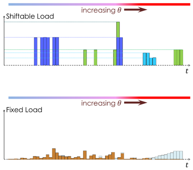
Figure 2.
Tradeoffs between resources when equal utility.
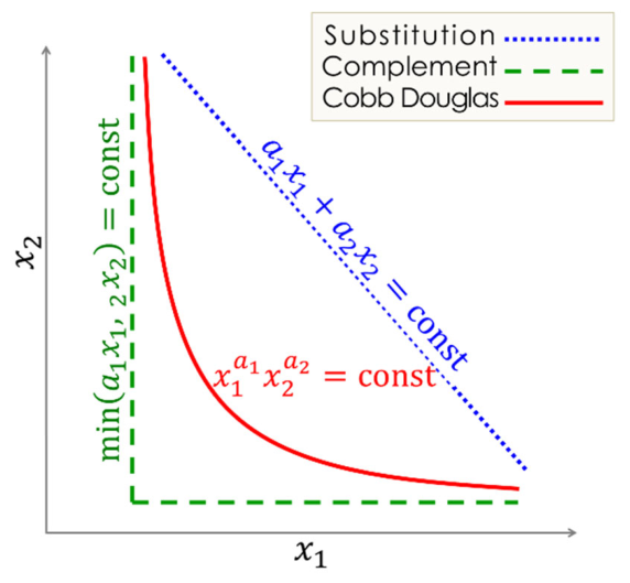
Figure 3.
Utility and cost as functions of load demand. As explained in the text, the fixed load is not sensitive to the unit cost of energy. (a) A nonlinear, saturating utility function. (b) The cost per unit load, which is also the slope of the utility function.
Figure 3.
Utility and cost as functions of load demand. As explained in the text, the fixed load is not sensitive to the unit cost of energy. (a) A nonlinear, saturating utility function. (b) The cost per unit load, which is also the slope of the utility function.
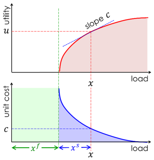
Figure 4.
Partial disaggregation in HUPDA. (a) Gaussian mixture of shiftable load at a time instant. (b) Non-negative factorization of the fixed load matrix.
Figure 4.
Partial disaggregation in HUPDA. (a) Gaussian mixture of shiftable load at a time instant. (b) Non-negative factorization of the fixed load matrix.
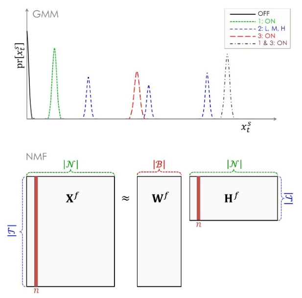
Figure 5.
Flowchart for model parameter estimation algorithm in SPUMA.
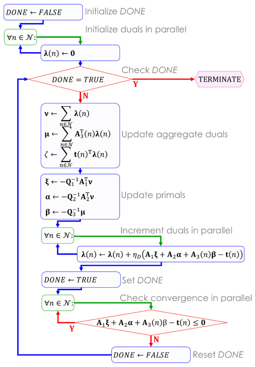
Figure 6.
Schematic showing the stages in the overall framework. (a) With separate monitoring of each load category. (b) With a single monitoring for the aggregate load.
Figure 6.
Schematic showing the stages in the overall framework. (a) With separate monitoring of each load category. (b) With a single monitoring for the aggregate load.
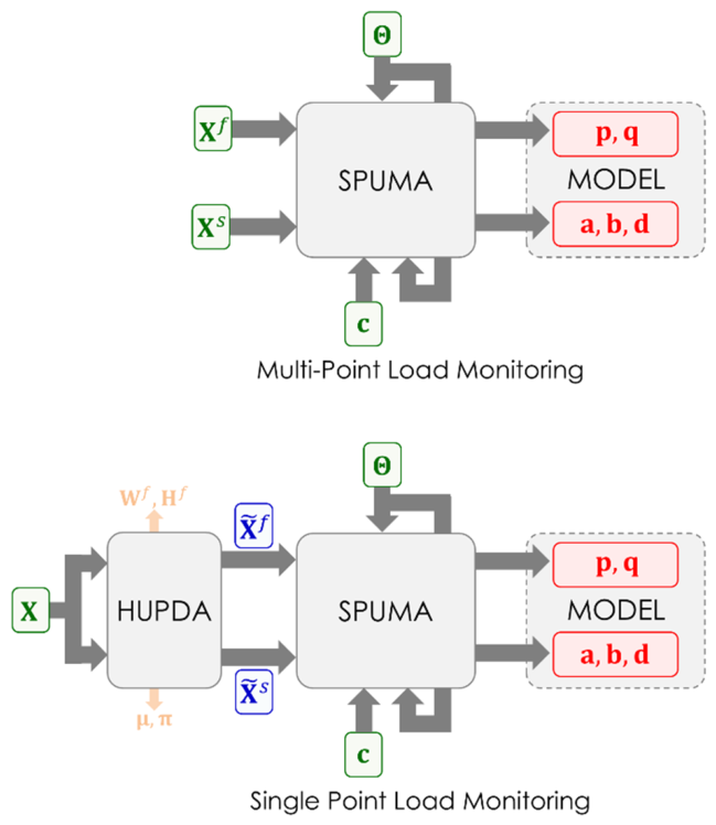
Figure 7.
Results obtained from SPUMA. The algorithm terminated within a total of 100 iterations with each dataset. The log scales in the x-axis and y-axis may be noted. (a) The plot shows the steadily increasing dual function with iteration, demonstrating the primal (i.e., loss) function’s progress towards the constrained optima. (b) The plot shows the steady decrease in the inequality constraint.
Figure 7.
Results obtained from SPUMA. The algorithm terminated within a total of 100 iterations with each dataset. The log scales in the x-axis and y-axis may be noted. (a) The plot shows the steadily increasing dual function with iteration, demonstrating the primal (i.e., loss) function’s progress towards the constrained optima. (b) The plot shows the steady decrease in the inequality constraint.
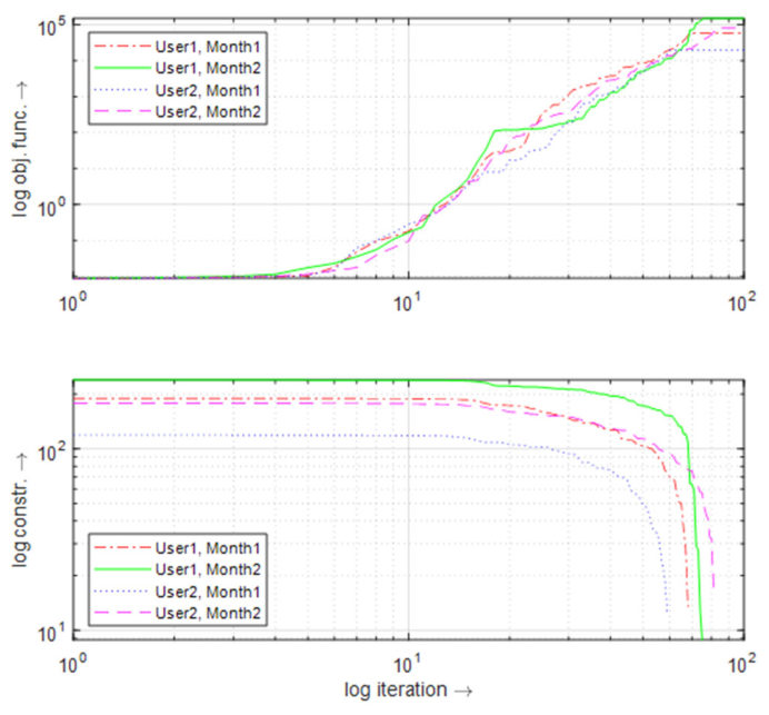
Figure 8.
Model parameters at each hour in the day.
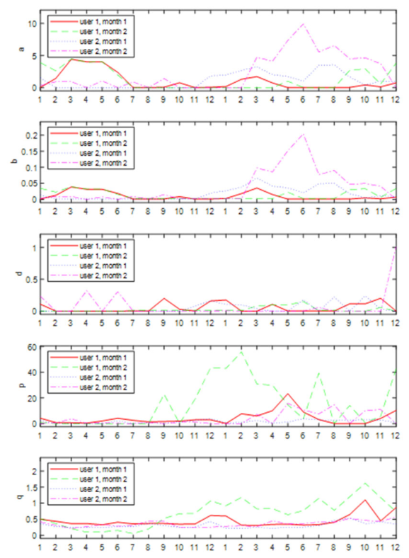
Figure 9.
Scatter plots of model parameters of the shiftable loads at each hour in . The points in each dataset are plotted using distinct shapes and colors. (a) Model parameter . (b) Model parameter. (c) Model parameter .
Figure 9.
Scatter plots of model parameters of the shiftable loads at each hour in . The points in each dataset are plotted using distinct shapes and colors. (a) Model parameter . (b) Model parameter. (c) Model parameter .
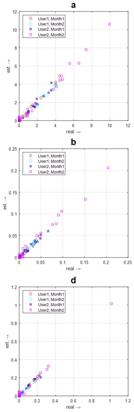
Figure 10.
Scatter plots of model parameters of the shiftable loads at each hour in . The points in each dataset are plotted using distinct shapes and colors. (a) Parameter . (b) Parameter.
Figure 10.
Scatter plots of model parameters of the shiftable loads at each hour in . The points in each dataset are plotted using distinct shapes and colors. (a) Parameter . (b) Parameter.
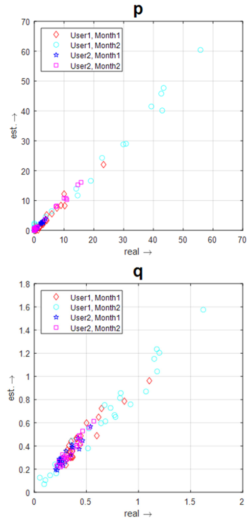
Figure 11.
Typical shiftable load usage patterns reproduced by the trained semi-parametric model using real unit cost and temperature data (blue lines). The lightly shaded regions are the ranges of the true values of these loads in the datasets, reflecting their large variability.
Figure 11.
Typical shiftable load usage patterns reproduced by the trained semi-parametric model using real unit cost and temperature data (blue lines). The lightly shaded regions are the ranges of the true values of these loads in the datasets, reflecting their large variability.
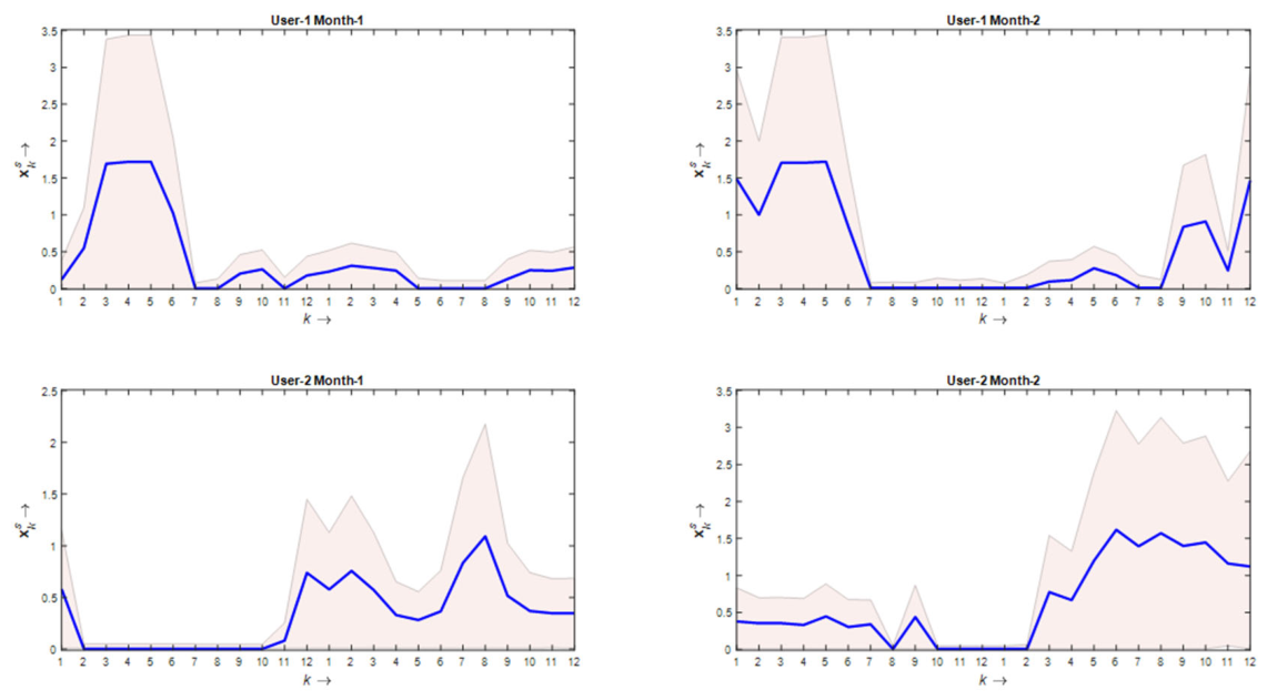
Figure 12.
Typical fixed load usage patterns reproduced by the trained semi-parametric model using real unit cost and temperature data (blue lines). The shaded regions are the ranges of the true values of these loads in the datasets, reflecting their large variability.
Figure 12.
Typical fixed load usage patterns reproduced by the trained semi-parametric model using real unit cost and temperature data (blue lines). The shaded regions are the ranges of the true values of these loads in the datasets, reflecting their large variability.
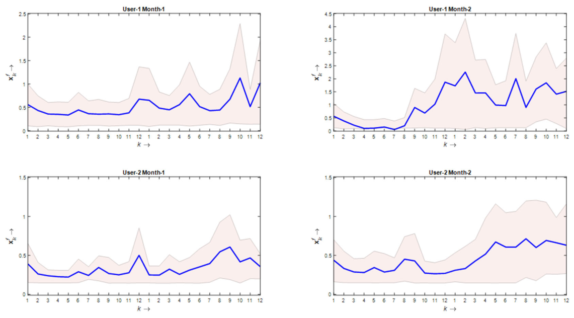

Table 1.
Weights of error and regularization functions, and constraint tolerance bounds.
| Error | Regularization | Constraint | ||||||
Table 2.
Loss terms, error norms, and computer time used to run SPUMA.
| Sample | User | 1 | 1 | 2 | 2 |
| Month | 1 | 2 | 1 | 2 | |
| Loss (raw) |
982.42 | 330.53 | 2421.28 | 1348.03 | |
| 4.28 | 0.44 | 55.87 | 4.11 | ||
| Loss (scaled) |
327.48 | 110.18 | 807.09 | 449.34 | |
| 6.59 | 0.68 | 85.96 | 6.32 | ||
| Loss (per sample) |
44.66 | 15.02 | 115.30 | 64.19 | |
| 0.19 | 0.02 | 2.66 | 0.20 | ||
| Error (raw) |
157.66 | 95.56 | 197.09 | 195.54 | |
| 96.09 | 39.63 | 259.98 | 66.41 | ||
| Error (% of load) |
15.70% | 27.59% | 23.56% | 23.39% | |
| 9.57% | 11.44% | 31.08% | 7.94% | ||
| Time in ms | - | 2313.94 | 7420.08 | 5297.99 | 4236.05 |
Disclaimer/Publisher’s Note: The statements, opinions and data contained in all publications are solely those of the individual author(s) and contributor(s) and not of MDPI and/or the editor(s). MDPI and/or the editor(s) disclaim responsibility for any injury to people or property resulting from any ideas, methods, instructions or products referred to in the content. |
© 2026 by the authors. Licensee MDPI, Basel, Switzerland. This article is an open access article distributed under the terms and conditions of the Creative Commons Attribution (CC BY) license (http://creativecommons.org/licenses/by/4.0/).
Copyright: This open access article is published under a Creative Commons CC BY 4.0 license, which permit the free download, distribution, and reuse, provided that the author and preprint are cited in any reuse.


