

Submitted:
02 July 2026
Posted:
03 July 2026
You are already at the latest version
Abstract
Object detection systems based on the You Only Look Once (YOLO) family have achieved strong performance under controlled conditions, but their reliability often deteriorates when input images are corrupted by sensor noise, low-light artifacts, or transmission errors. This study evaluates the impact of Gaussian noise on YOLO-based object detection and examines whether image denoising combined with model retraining can recover the lost robustness. Five YOLO variants (v8m–v12m) were trained on the PnPLO human-detection dataset (1,339 images) and tested under Gaussian noise at σ ∈ {0, 1, 5, 10, 20, 30}. Six denoising techniques—Gaussian Filter, BM3D, DnCNN, Autoencoder, CAE+PSO, and a no-denoising baseline—were then applied prior to retraining, and performance was re-measured on the noisy test set under a unified three-stage protocol covering clean training, noisy inference, and denoised retraining. Results show a moderate but consistent degradation across all metrics as σ increases. The denoising-plus-retraining pipeline restores performance most effectively for BM3D and DnCNN, while Autoencoder-based methods degrade detection further, with ∆mAP@50 ranging from −0.0049 for BM3D to −0.0351 for Autoencoder. These findings clarify the trade-off between noise suppression and structural preservation, underscoring the central role of feature integrity in noise-robust detection and providing a practical framework for deploying YOLO detectors in real-world imaging applications.
Keywords:
object detection
; YOLO
; Gaussian noise
; image denoising
; robustness analysis
; noise-aware training
1. Introduction
Object detection plays a core role in many practical artificial intelligence systems, such as security surveillance, intelligent transportation, autonomous robots, and computer vision systems in uncontrolled environments [1]. In recent years, deep learning-based object detection models, especially one-stage architectures like You Only Look Once (YOLO), have made significant strides in speed and accuracy, enabling efficient deployment in real-time systems [2,3]. While achieving high performance on standard datasets under ideal conditions, YOLO models are often trained and evaluated on clean data, which fails to fully reflect the common image-quality degradation encountered in practice [4]. One of the most common forms of degradation is Gaussian noise, which arises from sensor hardware limitations, low-light conditions, and data transmission and compression processes. Gaussian noise can severely degrade feature extraction and object localization capabilities, directly impacting the reliability of object detection systems in engineering applications. From an engineering perspective, ensuring robustness under noisy visual conditions is critical for reliable system deployment [5,6].
Previous studies have addressed the robustness of deep learning models in the face of image noise and data distortion [7]. However, most of these studies have focused on image classification or the use of two-stage detection architectures, while YOLO models, widely used in real-time applications, have not been systematically evaluated under the influence of Gaussian noise. Many studies have only evaluated a single dataset or a fixed noise level, leading to conclusions lacking generality [8,9]. Methods for improving model robustness often focus on data augmentation with noise or adversarial training techniques, while image denoising strategies combined with retraining object detection models have not been fully exploited [10]. There is a lack of comprehensive studies evaluating the impact of Gaussian denoising on the performance of YOLO models across various datasets, as well as analyzing the degree of performance recovery after retraining. Besides recent studies evaluating the robustness of computer vision models based on degraded benchmark datasets such as ImageNet-C or COCO-C, most of these studies primarily focus on image classification problems or evaluations of specific object detection architectures under general data distortion conditions. Meanwhile, the experimental framework of this study focuses on a systematic analysis of the sensitivity of several modern YOLO versions to a specific type of noise, namely Gaussian noise, in the context of a person detection problem. Unlike common corruption benchmarks that directly assess model performance degradation, this study not only analyzes the degree of model performance degradation under different noise levels but also evaluates performance recovery through a combined strategy of image denoising and model retraining. This approach allows for a deeper analysis of the relationship between data noise levels, the adaptability of the YOLO architecture, and the effectiveness of input data processing strategies to improve the robustness of object detection systems in real-world environments with unstable image quality. Given these limitations, this study raises the following main research questions: (1) How does Gaussian noise affect the performance of YOLO-based object detection models on different datasets? (2) Does the degree of performance degradation of YOLO depend on the characteristics of the dataset? (3) Can applying Gaussian denoising combined with retraining improve the robustness and performance of YOLO under noisy data conditions?
To answer the above questions, the goal of this study is to build a systematic experimental pipeline to evaluate and improve the robustness of YOLO models under the influence of Gaussian noise. Specifically, the study trains and evaluates YOLO on clean data, analyzes the level of performance degradation on Gaussian-noise data, and proposes a Gaussian denoising strategy combined with retraining to improve object detection performance in non-ideal data environments. The main contributions of this study include: (i) a systematic experimental evaluation of the robustness of YOLO-based object detection models under the influence of Gaussian noise on various common datasets; (ii) an analysis of the differences in performance degradation between datasets with different characteristics; and (iii) demonstrating the effectiveness of a Gaussian denoising strategy combined with retraining in improving YOLO performance on noisy data. In terms of application, this research offers significant practical value for the deployment of object detection systems in real-world environmental conditions where image quality is often unreliable. The results and analyses presented in this paper can provide a scientific basis for designing more robust object detection systems, especially in engineering applications requiring high reliability and stable operation in noisy environments. The remainder of this paper is organized as follows. Section 2 reviews prior work on YOLO-based object detection, benchmark datasets, the impact of image noise on detection performance, robustness evaluation of deep learning models, and image denoising techniques for Gaussian noise, and synthesizes the research gap addressed in this study. Section 3 presents the proposed methodology, including the PnPLO dataset preparation, the YOLO detection algorithm, the evaluation metrics, the Gaussian noise generation procedure, and the denoising-plus-retraining strategy. Section 4 reports the experimental results across three stages—baseline performance on clean data, performance degradation under varying Gaussian noise levels, and performance recovery after denoising and retraining—together with a comparative analysis of six denoising methods applied to five YOLO variants. Section 5 discusses the implications of these findings, the differing robustness of YOLO versions, and the trade-off between noise suppression and structural feature preservation. Finally, Section 6 summarizes the main contributions, outlines practical implications, and suggests directions for future research.
2. Related Works
This section synthesizes recent literature on YOLO-based object detection, evaluation under image-quality degradation, and denoising / noise-aware training, and identifies the gaps that motivate the present study.
2.1. YOLO-Based Object Detection Models and Recent Benchmarks
YOLO is a one-stage object detector that performs localization and classification in a single inference, offering a strong accuracy–latency trade-off suitable for real-time engineering applications such as surveillance, intelligent transport, and autonomous robotics [11,12]. Successive generations have introduced multi-scale feature extraction, anchor-free heads, and improved bounding-box regression losses [13], and now span at least YOLOv3 through YOLOv12 with diverse model sizes [14].
Numerous studies have demonstrated the effectiveness of YOLO in standard test environments where input data is high-quality and imaging conditions are controlled [15,16,17]. Jiang and Zhong evaluate YOLOv5–YOLOv11 across 33 datasets and 11 domains and report YOLOv11 as the strongest variant in 6 of 11 domains under clean data [15]. Jegham et al. benchmark YOLOv3–YOLOv12 (including YOLO11) on three datasets covering Traffic Signs, African Wildlife, and Ships & Vessels, and conclude that YOLO11 offers the best accuracy–efficiency balance among modern variants [16]. Sapkota et al. report mAP@50 up to for the strongest configurations (YOLOv9 GELAN-base/-e), with YOLO11s at and YOLOv12l at on a fruitlet detection dataset under clean orchard conditions [17]. Robustness-oriented evaluations have only recently begun: Gholinavaz et al. test YOLOv5s, YOLOv8m, YOLOv10n, and Faster R-CNN on the DAWN traffic dataset under fog, rain, Gaussian, and salt-and-pepper noise, with YOLOv8m reaching mAP@50 = 0.712 on clean data and degrading to mAP@50 = 0.639 under Gaussian noise and blur [18]; Apostolidis et al. benchmark YOLOv3–v11 and YOLOX on MS COCO with adversarial and corruption perturbations, and find that older variants (v3, v4) tolerate Gaussian noise better than newer ones [19]; Nabahirwa et al. compare YOLOv8–v12 on the underwater DUO and Roboflow100 datasets (∼10 000 images) and observe that YOLOv12 leads on clean data but is highly vulnerable to noise [20]. Table 1 summarizes these benchmarks alongside the present study.
2.2. Image Quality Degradation and Detection Robustness
Real-world deployment exposes object detectors to image-quality degradations such as Gaussian and salt-and-pepper noise, motion blur, and lighting variations [21,22]. These distortions impair feature extraction and bounding-box regression, especially for small or low-contrast objects [23,24]. Standard datasets such as MS COCO and Pattern Analysis, Statistical Modelling and Computational Learning - Visual Object Classes (PASCAL VOC), while widely used to compare detectors under clean conditions [25,26,27], were largely collected under near-ideal conditions and only partially capture this practical setting. Robustness-oriented benchmarks such as ImageNet-C, COCO-C, and ObjectNet apply controlled corruptions to measure performance degradation [28,29,30]. However, these benchmarks were primarily constructed for image classification and two-stage detectors; systematic evaluation of one-stage detectors like YOLO under Gaussian noise across multiple datasets remains scarce [31,32,33].
2.3. Denoising Preprocessing and Noise-Aware Training Strategies
Two complementary directions have been explored to improve detector robustness under degraded inputs. The first applies image denoising as a preprocessing step. Traditional methods such as Gaussian and median filters are simple and fast but tend to blur fine structures [34,35]. Block-matching methods (e.g. BM3D) and deep-learning-based denoisers (DnCNN, denoising autoencoders) achieve higher peak signal-to-noise ratio at the cost of higher complexity and reliance on training data [36,37]. Most denoising work targets pixel-level reconstruction quality rather than downstream detection performance [38]. The second direction is noise-aware training, where the detector is trained on noise-augmented data [39] or jointly with a denoising branch [40], but consistency across datasets and noise levels remains limited [41,42]. Combining the two approaches—denoising followed by detector retraining on the denoised distribution—has received less systematic attention.
2.4. Research Gap
Across the surveyed literature, three gaps remain. First, most robustness studies focus on image classification or two-stage detectors; one-stage YOLO models, despite their dominance in real-time deployment, have not been systematically evaluated under controlled Gaussian-noise sweeps. Second, the majority of evaluations use a single dataset or a fixed noise level, limiting generalizability. Third, the joint effect of denoising plus model retraining—rather than either in isolation—has not been quantified across multiple noise levels and denoising methods on the same YOLO family. The present study addresses these gaps with a unified pipeline that evaluates YOLOv8m–YOLOv12m on a multi-dataset setting under six Gaussian noise levels, six denoising methods, and a denoise-plus-retraining protocol, and reports performance recovery via mAP@50 against the noisy baseline.
3. Methodology
Figure 1 illustrates the research, which begins with collecting input images from a camera and using optical merging techniques to build an image set (such as pedestrian images). The YOLO model is then trained and evaluated on the original data, followed by the creation of Gaussian-noise data and the evaluation of its detection performance on this dataset. Finally, Gaussian noise reduction is applied, and the results are re-evaluated to analyze the impact of noise and the effectiveness of the proposed method.
3.1. Datasets Description and Preparation
Person and Person-Like Objects (PnPLO) is a specialized dataset for the human detection problem. This dataset includes “Person” samples taken from the VOC set, combined with hard negatives such as statues, mannequins, robots, and human-like objects. It also includes weather-enhanced composite samples, totaling 1339 images at variable native resolutions ranging from to pixels (most images approximately pixels), publicly available on Kaggle [43] (Figure 2). All images are resized to pixels at training time (Section 4, Table 2). PnPLO’s main contribution is its design to address semantic ambiguity, enabling the training of models capable of accurately distinguishing between real people and human-like objects in complex contexts.
In this study, the PnPLO dataset, consisting of 1339 images, was divided into three subsets for model training, testing, and evaluation purposes. Specifically, the data was split 70% for the training set, 15% for the validation set, and 15% for the test set. The data splitting was random but ensured a relatively even distribution among the object classes. During training, several data augmentation techniques were applied to improve the model’s generalizability, including horizontal image flipping, slight changes in brightness and contrast, and image scaling. Additionally, to ensure the reproducibility of the experiment, random parameters were fixed by establishing random seeds in the training environment.
3.2. YOLO-Based Object Detection Models
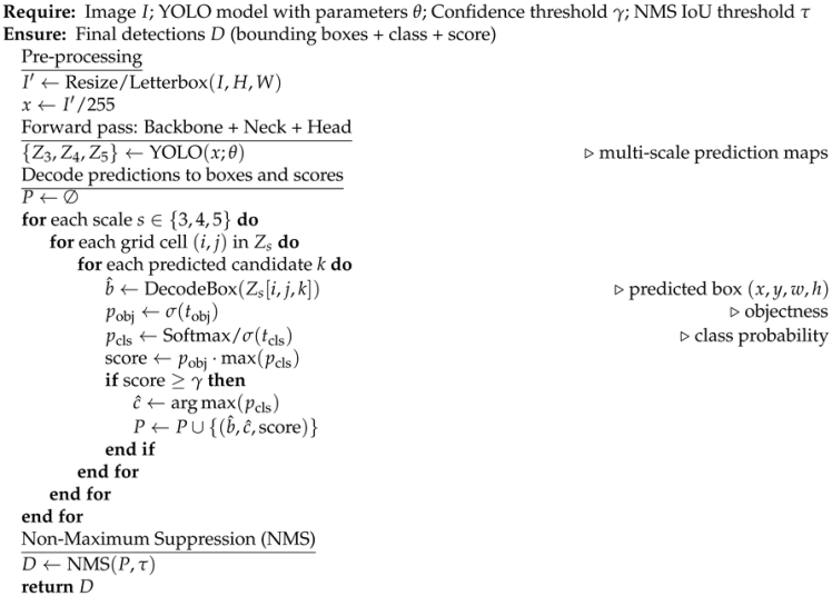
Algorithm 1 presents the YOLO-based object detection algorithm, which boasts the outstanding advantage of one-stage processing, allowing simultaneous object bounding box prediction and classification across multiple scales, enabling efficient detection of objects of varying sizes. The combination of objectness, class probability, and NMS reduces noise and eliminates duplicate predictions, improving overall accuracy. Thanks to its compact architecture and fast inference, YOLO is particularly suitable for real-time detection tasks such as pedestrian detection in complex environments.
| Algorithm 1 YOLO-based Object Detection (General Pseudo-code) |
 |
3.3. Baseline Performance Evaluation on Clean Data
Precision (Eq. 1), Recall (Sensitivity) (Eq. 2), Accuracy (Eq. 3), and Specificity (Eq. 4) are used to evaluate the predictive performance of the model based on True Positive (TP), True Negative (TN), False Positive (FP), and False Negative (FN) values. The F1-Score (Eq. 5) is a harmonic average between Precision and Recall, balancing the accuracy and object detection capability of the model. In the object detection problem, (Eq. 6) is calculated from the area under the Precision–Recall curve at the IoU threshold of 0.5, and is the average value of across all object classes. Additionally, (Eq. 7) is calculated as the average of mAP at IoU thresholds from 0.5 to 0.95 (step 0.05) for a more comprehensive model evaluation.
where TP: The model correctly predicts a positive object. TN: The model correctly predicts a negative case (no object). FP: The model incorrectly predicts an object when there is none. FN: The model fails to detect an actual object.
where is Precision as a function of Recall, C is the number of object classes, and IoU = 0.5 is the evaluation threshold.
3.4. Gaussian Noise Generation
In this study, Gaussian noise is used to simulate random noise commonly occurring during image acquisition and transmission, such as sensor noise, poor lighting conditions, or electronic noise. The addition of Gaussian noise to the original image aims to evaluate the robustness of the YOLO model in pedestrian detection when image quality degrades. Mathematically, Gaussian noise is assumed to follow a normal distribution with an expected value of 0 and a variance of , represented as . The noisy image (Eq. 8) is created by adding noise to the original image :
where is the noise value at pixel .
The parameter determines the level of noise, with a larger indicating a greater degradation of image quality. By varying the value of , the study can analyze the impact of different noise levels on the detection performance of YOLO, thereby evaluating the adaptability and stability of the model under complex real-world conditions.
3.5. Robustness Evaluation on Gaussian Noisy Data
After evaluating the baseline performance of the YOLO model on clean data, the study proceeded to assess the robustness of the model under conditions of data degradation due to Gaussian noise. Specifically, images in the PnPLO dataset were supplemented with Gaussian noise at different variance levels , creating corresponding noisy datasets. The YOLO model trained on clean data was used directly to infer on these noisy datasets without further parameter adjustments. Pedestrian detection performance was evaluated using the Precision, Recall, mAP@50, and mAP@50–95 indices, thereby analyzing the degree of performance degradation as noise levels increase. The evaluation results reflect the generalizability and sensitivity of the YOLO model to common noisy conditions in real-world environments.
3.6. Denoising Methods and Retraining Strategy
To improve detection performance under noisy conditions, this study evaluates six denoising methods covering classical, transform-domain, and deep-learning paradigms, each followed by retraining the YOLO detector on the denoised distribution. The six methods are: a no-denoising baseline, Gaussian Filter, BM3D, a Denoising Autoencoder, DnCNN, and a Convolutional Autoencoder optimized by Particle Swarm Optimization (CAE+PSO). All learning-based denoisers are trained on patches of pixels (4 random patches per training image) using the Adam optimizer with learning rate , mean-squared-error loss, and a ReduceLROnPlateau scheduler (patience 5, factor ); training is performed for 50 epochs per noise level with mixed-precision (AMP) on a single A100 GPU. At inference, deep models are applied with a sliding-window scheme of patch size and stride 112 with overlap averaging. The five non-baseline methods are described below.
3.6.1. Gaussian Filter
A two-dimensional Gaussian kernel is convolved with each input image to suppress high-frequency noise while preserving low-frequency structure. Filtering uses the OpenCV GaussianBlur routine with kernel size adapted to the noise level: for , for , for , and for higher noise levels; the spread is set automatically from the kernel size. This method has no learnable parameters.
3.6.2. BM3D
Block-Matching and 3D filtering applies collaborative filtering on three-dimensional groups of similar image blocks. The colour variant bm3d.bm3d_rgb is used; the noise standard deviation is set to (clamped at a minimum of to avoid degenerate cases) and the default profile is retained. As with the Gaussian filter, BM3D has no trainable parameters.
3.6.3. Denoising Autoencoder
A symmetric convolutional encoder-decoder is trained to reconstruct the clean patch from its noisy counterpart. The encoder stacks two convolutions () followed by max-pooling, then two more () followed by max-pooling, with ReLU activations throughout. The decoder mirrors this with transposed convolutions () and a final sigmoid. One model is trained per noise level using the common training schedule above.
3.6.4. DnCNN
A residual deep convolutional denoiser following Khmag [36] is implemented with 17 convolutional layers, 64 feature channels per layer, and kernels. The first layer uses Conv + ReLU; the next 15 layers use Conv + BatchNorm + ReLU; the final layer is a Conv predicting the noise residual, so that the denoised output is computed as . As with the Autoencoder, one DnCNN model is trained per noise level using the common training schedule above.
3.6.5. CAE+PSO
A Convolutional Autoencoder with Batch Normalisation is parametrised by three hyperparameters—learning rate, base number of feature channels, and convolution kernel size—which are searched by Particle Swarm Optimization. The architecture follows an encoder of two stages doubling the channel count and using max-pooling, mirrored by a decoder with transposed convolutions and a final sigmoid. PSO uses 6 particles over 10 iterations with inertia weight decreasing linearly from to and acceleration coefficients ; each particle’s fitness is the validation MSE after 8 short training epochs. Search bounds are , , and . The best particle is then trained for the full 50-epoch schedule.
Retraining protocol.
After denoising, each -specific denoised dataset is used to retrain the corresponding YOLO variant from the clean checkpoint, using the same Ultralytics training configuration as the clean baseline (Section 4, Table 2). This denoise-plus-retrain pipeline allows the detector to learn features that are stable under the post-denoising distribution rather than relying solely on the clean distribution. Performance is then re-measured on the matching noisy test split as described in Section 3.7.
3.7. Performance Re-Evaluation on Gaussian Noisy Data
After applying denoising and retraining, the YOLO model was re-evaluated on Gaussian noisy datasets corresponding to different levels. Precision, Recall, mAP@50, and mAP@50–95 metrics were used to compare performance across the three cases: clean data, unprocessed noisy data, and denoised noisy data. This comparison allows for a clear assessment of the effectiveness of the denoising and retraining steps, demonstrating the ability to improve the accuracy and robustness of the YOLO model under Gaussian noise conditions. The results confirm that the proposed strategy helps the model maintain more stable performance, making it suitable for pedestrian detection applications in complex real-world environments.
4. Experimental Results
The study clearly presents the performance evaluation process of YOLO models through three stages: clean data, Gaussian-noised data, and after denoising combined with retraining. To ensure the reliability of experimental results, the study also performed statistical analysis to assess the stability of the model evaluation metrics. Specifically, each model training and evaluation experiment was repeated multiple times with the same parameter configuration, and the average values of Accuracy, Precision, Recall, F1-score, mAP50, and mAP50–95 were used to report the final results. Simultaneously, a 95% confidence interval was calculated for the key metrics to assess the variability of results between experimental runs. This analysis allowed for the determination of whether the observed performance improvements between models and different data conditions were statistically significant, thereby increasing the reliability of the conclusions drawn from the experiments. The results show that model performance gradually decreases as noise levels increase, but improves significantly after denoising and retraining, demonstrating the effectiveness of the proposed method in increasing the stability of object detection systems under degraded data conditions.
In presenting the experimental results, figures were selected to visually demonstrate the performance trends of the YOLO models under different Gaussian noise levels, as well as after applying noise reduction and retraining strategies. To avoid duplication of information between data tables and figures, the study retained only those figures that most clearly illustrate the changing trends of the evaluation metrics and model behavior under different data conditions. Figures with content similar to the data tables were simplified or omitted to make the results more concise, while still providing sufficient information for analyzing and comparing the performance of the models.
4.1. Experimental Setup and Evaluation Metrics
Hardware setup: This configuration is designed for pedestrian recognition problems requiring high accuracy and stable operation in complex environments. The combination of high-performance GPU hardware and optimized hyperparameters enables stable convergence and efficient feature learning for reliable pedestrian detection and classification (Table 2).

Table 2.
Training Configuration for Pedestrian Recognition Model.
| Parameter Group | Component | Configuration Value |
|---|---|---|
| Software | Ultralytics | 8.3.154 |
| Python | 3.11.13 | |
| PyTorch (Torch) | 2.5.1 | |
| CUDA | 12.1 | |
| Hardware | GPU | NVIDIA GeForce RTX 4090 |
| GPU Memory | 24,564 MB (∼24GB VRAM) | |
| Training Configuration | Number of epochs | 500 |
| Input image size | 640 × 640 pixels | |
| Batch size | 32 | |
| Optimizer | SGD | |
| Initial learning rate | 0.01 |
Datasets: PnPLO [43] is a specialized dataset for the human detection problem, consisting of 1339 images, downloaded from Kaggle, combining “Person” patterns from VOCs with hard negatives such as statues, mannequins, robots, and human-like objects, along with weather-enhanced composite images. During training, several data augmentation techniques were applied to improve the model’s generalizability, including horizontal image flipping, slight changes in brightness and contrast, and image scaling.
Benchmark setup: The pedestrian recognition system benchmark setup is built on an NVIDIA GeForce RTX 4090 GPU with 24,564 MB (∼24GB VRAM), ensuring powerful computing capabilities for complex deep learning and feature extraction tasks. The 640 × 640 pixel input image size strikes a balance between detection accuracy and computational efficiency.
4.2. Baseline Performance on Clean Data
On clean data, Table 3 shows that YOLOv9m achieved the highest Accuracy (0.7812) and YOLOv12m achieved the highest Precision (0.8704), while YOLOv8m had the highest mAP@50 (0.8992) and mAP@50–95 (0.6613), indicating better overall detection capabilities compared to the other models. YOLOv8m also had the highest Sensitivity (0.8093) and F1-Score (0.7909), showing fairly stable object detection capabilities. Meanwhile, YOLOv12m achieved an F1-Score of 0.7852 and a sensitivity of 0.7871, while YOLOv10m had the lowest Accuracy (0.7474), indicating poorer overall performance compared to the other versions.
Figure 3 shows the per-epoch validation curves of mAP@50, mAP@50–95, Precision, and Recall during clean-data training of YOLOv8m–YOLOv12m. All five models converge within the configured 500-epoch budget under early stopping (patience 50), with the largest gains in the first 100–150 epochs and a flat plateau thereafter. YOLOv8m reaches the highest mAP@50 (∼89.9%) and mAP@50–95 (∼66.1%) of the family; YOLOv11m and YOLOv12m converge more slowly on mAP@50–95 (final values ∼62.0% and ∼62.8% respectively), suggesting that the additional capacity of the newer variants is not fully exploited at this dataset scale. Figure 4 summarises the same numbers as a heatmap across YOLO variants. YOLOv8m attains the highest overall mAP@50 (∼89.9%), with Precision ∼85.6%, Recall ∼85.2%, and F1-Score ∼79.1%; YOLOv12m yields the strongest Precision (∼87.0%) but lower Recall (∼80.3%), while YOLOv9m attains the highest Specificity (∼78.0%) and Accuracy (∼78.1%). Across the family, mAP@50 spans ∼87.7–89.9% and mAP@50–95 spans ∼62.0–66.1%, indicating consistent baseline performance on the original PnPLO dataset. Figure 5 shows qualitative detections on a representative clean image: YOLOv8m and YOLOv10m detect both persons with confidence approximately – and – respectively, while YOLOv9m and YOLOv12m detect only one person at higher confidence (∼–); YOLOv11m detects both persons but with a lower confidence of ∼.
4.3. Performance Degradation Under Gaussian Noise
In this study, Gaussian noise was applied to the PnPLO dataset at , and 30 to evaluate the system’s robustness under image-quality degradation.
Table 4 shows the performance of the YOLO models as a function of Gaussian noise levels from 0–30. Without noise (), YOLOv9m achieved the highest Accuracy (0.7812) and YOLOv8m achieved the highest F1-Score (0.7909), mAP@50 (0.8992), and mAP@50–95 (0.6613). At moderate noise (), YOLOv8m remained the best with Accuracy = 0.7892 and mAP@50 = 0.8905. When noise levels are high (–30), all models experience gradual performance degradation. YOLOv8m and YOLOv11m demonstrated the best noise resilience, with Accuracy drops of only 0.0152 and 0.0151 respectively across the full noise range.
Figure 6 traces how each detection metric evolves as the Gaussian noise level increases from to , with one curve per YOLO variant. The four panels reveal that the metrics most sensitive to noise are mAP@50–95 and Recall, which fall monotonically across the family, whereas Precision is comparatively flat: for example, YOLOv10m loses ∼ percentage points of mAP@50 (from ∼ at to ∼ at ) and ∼ points of Recall (∼ to ∼), while YOLOv8m loses only ∼ points of mAP@50 (∼ to ∼) and even briefly increases Precision to ∼ at before declining at . The curves also show that variant orderings are not stable across : YOLOv8m and YOLOv12m alternate in leading mAP@50 at low noise, while at the spread between the best and worst variant compresses below points. Figure 7 re-presents the same data as a (variant ) heatmap per metric, which makes the cross-variant comparison at any single easier to read. Reading the mAP@50 panel by column shows YOLOv8m occupying the warmest cell at every (∼ at down to ∼ at ), while the remaining four variants form a tight band around 84– throughout. The mAP@50–95 panel shows a similar dominance of YOLOv8m (∼ at , ∼ at ), with YOLOv11m the coolest column. Precision and Recall remain in narrow bands of 88– and 84– respectively, with YOLOv8m at ∼ Precision and ∼ Recall at . Figure 8 provides a qualitative view: at low noise (–5) most variants detect both persons with confidence ∼–, whereas at –30 several variants drop to a single detection and confidence collapses to ∼–, illustrating the metric-level decline in concrete failure cases.
4.4. Performance Improvement After Denoising and Retraining
Table 5 shows that after Gaussian-Filter denoising and retraining, the performance of the YOLO models improves and remains fairly stable. At , YOLOv9m achieved the highest Accuracy (0.7812) and YOLOv12m the highest Precision (0.9190), while YOLOv8m attained the highest F1-Score (0.7909) and mAP@50 (0.8992). At low to medium noise levels (–10), the models maintain good performance; for example, YOLOv9m reaches Accuracy 0.7932 and F1-Score 0.8030 at , and YOLOv11m reaches Sensitivity 0.8287 at . At , YOLOv10m improves Accuracy to 0.7637, illustrating the benefit of the denoising step. As noise increases (–30), performance declines moderately; YOLOv8m Accuracy decreases from 0.7634 to 0.7388 and mAP@50 from 0.8992 to 0.8439, whereas YOLOv9m remains relatively stable with Accuracy 0.7696 at and mAP@50 around 0.8726, indicating better post-denoising adaptation to noisy data.
Figure 9 shows that as the noise level increases from = 0 to = 30, the performance of the YOLO models gradually decreases; for example, YOLOv8m decreases mAP@50 from 0.899 to 0.844 and mAP@50–95 from 0.661 to 0.588. Other models also show a similar trend, such as YOLOv9m decreasing mAP@50 from 0.885 to 0.846 and mAP@50–95 from 0.634 to 0.566, while YOLOv10m decreases from 0.876 to 0.836 (mAP@50). Notably, YOLOv11m was strongly affected at = 5 with mAP@50 of only 0.860 and mAP@50–95 of 0.596, indicating high sensitivity to noise compared to the other models. Figure 10 shows the heatmap evaluating the performance of YOLO (v8m–v12m) models after noise reduction using a Gaussian filter with noise levels from 0 → 30, where the highest values are 0.899 (YOLOv8m, =0) and 0.889 (YOLOv9m, =1). As the noise level increases, the performance of most models gradually decreases; for example, YOLOv8m decreased from 0.899 to 0.844, YOLOv10m from 0.877 to 0.836, and YOLOv12m from 0.891 to 0.836 as increased to 30. The lowest value in the table is 0.832 (YOLOv11m, =30), indicating that high noise significantly reduced accuracy, although most models maintained performance around 0.83–0.90. Figure 11 illustrates the original (clean) image and different Gaussian noise levels with values = 0, 1, 5, 10, 20, and 30 to evaluate the object detection efficiency after noise reduction. As increases from 0 to 30, the noise level in the image increases significantly, especially from = 10 onwards, the image begins to become heavily grainy and detail decreases. However, after noise reduction, the object detection system still maintains its recognition capability at low levels (0–5) and gradually declines when reaches 20–30.
Comparison across the six denoising methods. Beyond the Gaussian-Filter results above, the same denoise-plus-retraining pipeline was applied with the no-denoising baseline, BM3D, Autoencoder, DnCNN, and CAE+PSO to compare their effect on detection performance across the YOLO family. Figure 12 plots mAP@50 of YOLOv8m–YOLOv12m versus noise level for each method. At low noise (–1), most models reach approximately – mAP@50 (e.g. YOLOv8m , YOLOv9m , YOLOv12m ). As noise increases to –20, mAP@50 decreases noticeably; Autoencoder and CAE+PSO drop to ∼–, while DnCNN and the Gaussian Filter remain higher at ∼–. A notable outlier is YOLOv11m with BM3D at (mAP@50 ). At the methods continue to decline (∼–, e.g. YOLOv10m –, YOLOv12m –). Figure 13 re-presents this surface as per-method heatmaps over the (YOLO variant, ) grid: in the no-denoising panel mAP@50 spans ∼– at and ∼– at . BM3D and DnCNN sit closest to the no-denoising surface (BM3D + YOLOv9m reaches at ; DnCNN remains ∼– at –10 and ∼– at ), whereas Autoencoder and CAE+PSO show visibly cooler cells at high (e.g. YOLOv12m + Autoencoder at ). Figure 14 aggregates the same data over noise levels: the highest method-averaged mAP@50 is (YOLOv8m and YOLOv9m), followed by YOLOv12m (), YOLOv11m (), and YOLOv10m (); for mAP@50–95 the order is YOLOv8m (), YOLOv9m (), YOLOv10m (), YOLOv12m (), and YOLOv11m (). Figure 15 reports mAP@50 of each denoiser relative to the no-denoising baseline, computed as the mean over the noisy levels and averaged across the five YOLO variants: BM3D , Gaussian Filter , DnCNN , CAE+PSO , and Autoencoder . Finally, Figure 16 shows qualitative detections at after each denoiser; BM3D, DnCNN, and the Gaussian Filter retain stable detections across most YOLO variants, whereas the Autoencoder occasionally produces zero detections, consistent with its position at the bottom of the mAP@50 ranking.
5. Discussion
The results of this study show that Gaussian noise significantly affects the performance of YOLO-based object detection models. As the noise level increases from to , most variants show a marked decrease in evaluation metrics such as Accuracy, F1-Score, and mAP. For example, the Accuracy of YOLOv8m decreases from to , while the F1-Score of YOLOv11m decreases from to , indicating that image noise degrades the feature extraction capabilities of the underlying convolutional backbones and induces errors in both classification and bounding-box regression. This trend is consistent with prior work in computer vision in which image noise distorts feature structure and reduces foreground-background separability.
A notable finding in the experimental results is the varying sensitivity to noise among different YOLO versions. Variants such as YOLOv9m show better stability as noise increases, maintaining an Accuracy of around at , while other variants degrade more sharply. The differences in robustness across YOLO versions can be partly explained by architectural choices: newer variants employ richer multi-scale feature extraction and improved backbone/neck designs that aggregate contextual information from several feature levels, dampening the impact of high-frequency noise on the most informative features.
In the case of Gaussian noise, noise components often appear as random variations at high frequencies, while structural features of the object such as shape, edges, and contrast areas tend to exist at more stable feature levels. Therefore, models with stronger feature learning capabilities at various levels of abstraction will be less affected by noise, leading to more stable object detection performance under degraded data conditions. This can be explained by differences in network architecture, particularly the multi-scale feature extraction mechanisms and improved optimization strategies in newer YOLO versions. These improvements help the models learn more stable features in response to variations in input data.
Beyond evaluating the impact of noise, the study also demonstrates the effectiveness of denoising combined with model retraining. After this preprocessing step, the performance of the models improves and remains more stable in a degraded data environment. For example, YOLOv8m attains mAP@50 on clean data and most variants maintain comparatively stable performance as noise rises, indicating that denoising before training preserves features that the detector can subsequently learn to rely on.
Another important finding is that although noise reduction improves performance, when noise levels are very high (), model performance still degrades somewhat. This reflects the trade-off between noise removal and image feature preservation, as traditional noise reduction filters sometimes also lose important object details. Therefore, choosing an appropriate noise reduction method is a crucial factor in designing object detection systems operating in real-world environments. From an application perspective, the research results offer significant practical implications for deploying object detection systems in uncontrolled environments, where image data is often affected by sensor noise, low light, or complex environmental conditions. The evaluation process proposed in the study can be used as a reference framework to test the robustness of computer vision models against various forms of data degradation.
5.1. Comparison with Existing Robustness Enhancement Strategies
The denoising-plus-retraining results in Section 4 (Figure 12, Figure 13, Figure 14, Figure 15 and Figure 16) reveal a clear hierarchy among the six methods evaluated. BM3D (mAP@50 ) and the Gaussian Filter () preserve performance closest to the noisy baseline, indicating that lightweight or transform-domain methods that retain the underlying spatial structure of the image are the most compatible with YOLO’s feature extractor. DnCNN () achieves a comparable but slightly weaker result, despite its higher modelling capacity. In contrast, the two methods that aggressively reshape image content—Autoencoder () and CAE+PSO ()—consistently degrade detection accuracy. This pattern is robust across all five YOLO variants (v8m–v12m): the average mAP@50 after denoising spans only – across the family, while the mAP@50 differences across methods span the full – range. The fact that the strongest denoiser by pixel-level reconstruction (Autoencoder) is also the worst by detection-level mAP@50 supports the central observation of this study: in a noise-robust object detection pipeline, fidelity of the structural cues that the detector relies on is more important than aggressive noise removal. This trade-off, which is invisible to PSNR-style evaluation of denoising in isolation, motivates evaluating denoisers jointly with the downstream detector. Relative to the existing robustness-enhancement literature reviewed in Section 2, which focuses primarily on noise-aware training or denoising in isolation, the present results suggest that the choice of denoiser interacts non-trivially with the detector’s representation, so that gains reported on PSNR alone do not transfer to detection performance.
6. Conclusion
This study presents a unified, three-stage experimental framework for evaluating the robustness of modern YOLO-based object detectors under Gaussian noise and for restoring lost performance through a denoise-plus-retraining pipeline. Across five YOLO variants (v8m–v12m), six noise levels (), and six denoising strategies, the experiments demonstrate that detection performance degrades smoothly with increasing noise—most visibly in mAP@50–95 and Recall—and that retraining on denoised data recovers a substantial fraction of the lost accuracy. Crucially, the recovery is not monotonic in the strength of the denoiser: methods that preserve the spatial structure of the input (BM3D, Gaussian Filter, DnCNN) close the gap to within mAP@50 to of the noisy baseline, whereas methods that aggressively reshape image content (Autoencoder, CAE+PSO) widen it to to . This ordering—inverse to typical pixel-level denoising quality—constitutes the central scientific contribution of the paper: in noise-robust detection, fidelity of the structural cues used by the detector matters more than aggressive noise removal, and denoisers should therefore be selected jointly with the downstream detector rather than in isolation.
From an engineering perspective, the results provide concrete guidance for deploying YOLO detectors in environments where image quality is unreliable, such as security surveillance, intelligent transportation, and autonomous robotics. The proposed framework can be reused as a reference protocol for testing other one-stage detectors against controlled image-quality degradations, and the structural-preservation criterion offers a quick filter for selecting denoisers in any pedestrian- or person-detection pipeline that must operate under sensor noise, low-light, or transmission-related corruption.
The study also has limitations that point to natural extensions. First, the experiments are confined to a single human-detection dataset (PnPLO) and to additive Gaussian noise; broader generalisation requires evaluating other corruptions (e.g. salt-and-pepper, motion blur, JPEG compression, low-light) and other domains (traffic, aerial, medical imagery). Second, the deep denoisers used here are trained per noise level using standard architectures; jointly trained or noise-aware detector backbones, as well as more recent transformer-based denoisers, were not evaluated and represent a promising direction for further closing the mAP@50 gap. Future work will integrate multiple noise types, additional datasets, and end-to-end noise-aware training schemes that are explicitly optimised for downstream detection rather than for pixel-level reconstruction quality.
References
- Cheng, G.; et al. Towards Large-Scale Small Object Detection: Survey and Benchmarks. IEEE Trans. Pattern Anal. Mach. Intell. 2023, 45, 13467–13488. [Google Scholar] [CrossRef] [PubMed]
- Mohammed, S.Y. Architecture review: Two-stage and one-stage object detection. Frankl. Open 2025, 12, 100322. [Google Scholar] [CrossRef]
- Chen, W.; Luo, J.; Zhang, F.; et al. A review of object detection: Datasets, performance evaluation, architecture, applications and current trends. Multimed. Tools Appl. 2024, 83, 65603–65661. [Google Scholar] [CrossRef]
- Vijayakumar, A.; Vairavasundaram, S. YOLO-based object detection models: A review and its applications. Multimed. Tools Appl. 2024, 83, 83535–83574. [Google Scholar] [CrossRef]
- Rodríguez-Rodríguez, J.A.; López-Rubio, E.; Ángel-Ruiz, J.A.; Molina-Cabello, M.A. The impact of noise and brightness on object detection methods. Sensors 2024, 24, 821. [Google Scholar] [CrossRef] [PubMed]
- Agnew, C.; Eising, C.; Denny, P.; Scanlan, A.; Van De Ven, P.; Grua, E.M. Quantifying the Effects of Ground Truth Annotation Quality on Object Detection and Instance Segmentation Performance. IEEE Access 2023, 11, 25174–25188. [Google Scholar] [CrossRef]
- Gui, S.; Song, S.; Qin, R.; Tang, Y. Remote sensing object detection in the deep learning era—A review. Remote Sens. 2024, 16, 327. [Google Scholar] [CrossRef]
- Kamath, V.; Renuka, A. Deep learning based object detection for resource constrained devices: Systematic review, future trends and challenges ahead. Neurocomputing 2023, 531, 34–60. [Google Scholar] [CrossRef]
- Amjoud, A.B.; Amrouch, M. Object Detection Using Deep Learning, CNNs and Vision Transformers: A Review. IEEE Access 2023, 11, 35479–35516. [Google Scholar] [CrossRef]
- Kumar, T.; Brennan, R.; Mileo, A.; Bendechache, M. Image Data Augmentation Approaches: A Comprehensive Survey and Future Directions. IEEE Access 2024, 12, 187536–187571. [Google Scholar] [CrossRef]
- Mustapha, A.A.; Yoosuf, M.S. Exploring the efficacy and comparative analysis of one-stage object detectors for computer vision: A review. Multimed. Tools Appl. 2024, 83, 59143–59168. [Google Scholar] [CrossRef]
- Yuan, M.; Zhang, C.; Wang, Z.; Liu, H.; Pan, G.; Tang, H. Trainable spiking-YOLO for low-latency and high-performance object detection. Neural Netw. 2024, 172, 106092. [Google Scholar] [CrossRef] [PubMed]
- Diwan, T.; Anirudh, G.; Tembhurne, J.V. Object detection using YOLO: challenges, architectural successors, datasets and applications. Multimed. Tools Appl. 2023, 82, 9243–9275. [Google Scholar] [CrossRef] [PubMed]
- Ali, M.L.; Zhang, Z. The YOLO framework: A comprehensive review of evolution, applications, and benchmarks in object detection. Computers 2024, 13, 336. [Google Scholar] [CrossRef]
- Jiang, T.; Zhong, Y. ODverse33: Is the New YOLO Version Always Better? A Multi-Domain Benchmark from YOLOv5 to YOLOv11. arXiv 2025, (v3, Apr. 2025 revision). arXiv:2502.14314. [Google Scholar] [CrossRef]
- Jegham, N.; Koh, C.Y.; Abdelatti, M.; Hendawi, A. YOLO Evolution: A Comprehensive Benchmark and Architectural Review of YOLOv12, YOLO11, and Their Previous Versions. arXiv 2024, (v4, Mar. 2025 revision). arXiv:2411.00201. [Google Scholar] [CrossRef]
- Sapkota, R.; Meng, Z.; Churuvija, M.; Du, X.; Ma, Z.; Karkee, M. Comprehensive Performance Evaluation of YOLOv12, YOLO11, YOLOv10, YOLOv9 and YOLOv8 on Detecting and Counting Fruitlet in Complex Orchard Environments. arXiv 2025, arXiv:2407.12040. (later published in Agricultural Communications, 2026, https://doi.org/10.1016/j.agrcom.2026.100125). [Google Scholar] [CrossRef]
- Gholinavaz, S.; Saeedi, N.; Gharehveran, S.S. Robustness Analysis of YOLO and Faster R-CNN for Object Detection in Realistic Weather Scenarios with Noise Augmentation. Sci. Rep. 2025, 15, 44888. [Google Scholar] [CrossRef] [PubMed]
- Apostolidis, K.D.; Papakostas, G.A. Delving into YOLO object detection models: Insights into adversarial robustness. Electronics 2025, 14, 1624. [Google Scholar] [CrossRef]
- Nabahirwa, E.; Song, W.; Zhang, M.; Chen, S. An Empirical Study on the Robustness of YOLO Models for Underwater Object Detection. arXiv 2025, arXiv:2509.17561. [Google Scholar] [CrossRef]
- Steffens, C.R.; Messias, L.R.V.; Drews, P.L.J.; Botelho, S.S.d.C. Can Exposure, Noise and Compression Affect Image Recognition? An Assessment of the Impacts on State-of-the-Art ConvNets. In Proceedings of the 2019 Latin American Robotics Symposium (LARS), 2019 Brazilian Symposium on Robotics (SBR) and 2019 Workshop on Robotics in Education (WRE), Rio Grande, Brazil, 2019; pp. 61–66. [Google Scholar] [CrossRef]
- Su, S.; Yan, Q.; Zhu, Y.; Sun, J.; Zhang, Y. From distortion manifold to perceptual quality: a data efficient blind image quality assessment approach. Pattern Recognit. 2023, 133, 109047. [Google Scholar] [CrossRef]
- Freire, A.; Silva, L.H.D.S.; de Andrade, J.V.; Azevedo, G.O.; Fernandes, B.J. Beyond clean data: Exploring the effects of label noise on object detection performance. Knowl.-Based Syst. 2024, 304, 112544. [Google Scholar] [CrossRef]
- Dai, Y.; Li, X.; Zhou, F.; Qian, Y.; Chen, Y.; Yang, J. One-Stage Cascade Refinement Networks for Infrared Small Target Detection. IEEE Trans. Geosci. Remote Sens. 2023, 61, 1–17. [Google Scholar] [CrossRef]
- Jamali, M.; Davidsson, P.; Khoshkangini, R.; et al. Context in object detection: a systematic literature review. Artif. Intell. Rev. 2025, 58, 175. [Google Scholar] [CrossRef]
- Er, M.J.; Chen, J.; Zhang, Y.; Gao, W. Research challenges, recent advances, and popular datasets in deep learning-based underwater marine object detection: A review. Sensors 2023, 23, 1990. [Google Scholar] [CrossRef] [PubMed]
- Liu, Y.; Sun, P.; Wergeles, N.; Shang, Y. A survey and performance evaluation of deep learning methods for small object detection. Expert Syst. With Appl. 2021, 172, 114602. [Google Scholar] [CrossRef]
- Lee, Y.; Kim, J. Robustness of deep learning models for vision tasks. Appl. Sci. 2023, 13, 4422. [Google Scholar] [CrossRef]
- Jamil, S. Review of image quality assessment methods for compressed images. J. Imaging 2024, 10, 113. [Google Scholar] [CrossRef] [PubMed]
- Paulin, G.; Ivašić-Kos, M. Review and analysis of synthetic dataset generation methods and techniques for application in computer vision. Artif. Intell. Rev. 2023, 56, 9221–9265. [Google Scholar] [CrossRef]
- Wan, Z.; Wang, Z.; Chung, C.; Wang, Z. A survey of dataset refinement for problems in computer vision datasets. ACM Comput. Surv. 2024, 56, 1–34. [Google Scholar] [CrossRef]
- Gallagher, J.E.; Oughton, E.J. Surveying You Only Look Once (YOLO) Multispectral Object Detection Advancements, Applications, and Challenges. IEEE Access 2025, 13, 7366–7395. [Google Scholar] [CrossRef]
- Arrington, M.N.; Scherf, K.S. Investigating the stability of individual differences in face recognition behavior. Sci. Rep. 2025, 15, 9425. [Google Scholar] [CrossRef] [PubMed]
- El-Shafai, W.; El-Nabi, S.A.; Ali, A.M.; et al. Traditional and deep-learning-based denoising methods for medical images. Multimed. Tools Appl. 2024, 83, 52061–52088. [Google Scholar] [CrossRef]
- Dalavai, L.; et al. Improving Deep Learning-Based Image Classification Through Noise Reduction and Feature Enhancement. In Proceedings of the 2024 International Conference on Artificial Intelligence and Quantum Computation-Based Sensor Application (ICAIQSA), Nagpur, India, 2024; pp. 1–7. [Google Scholar] [CrossRef]
- Khmag, A. Additive Gaussian noise removal based on generative adversarial network model and semi-soft thresholding approach. Multimed. Tools Appl. 2023, 82, 7757–7777. [Google Scholar] [CrossRef]
- Xiang, A.; Zhang, J.; Yang, Q.; Wang, L.; Cheng, Y. Research on splicing image detection algorithms based on natural image statistical characteristics. arXiv 2024, arXiv:2404.16296. [Google Scholar] [CrossRef]
- Jebur, R.S.; Der, C.S.; Hammood, D.A.; Weng, L.Y. Image denoising techniques: An overview. In Proceedings of the AIP Conference Proceedings; 2023; Vol. 2804, p. 020002. [Google Scholar] [CrossRef]
- Liu, J.; Wang, Z.; Ma, L.; et al. Benchmarking object detection robustness against real-world corruptions. Int. J. Comput. Vis. 2024, 132, 4398–4416. [Google Scholar] [CrossRef]
- Xiao, L.; Zhang, Z.; Huang, K.; Jiang, J.; Peng, Y. Noise Optimization in Artificial Neural Networks. IEEE Trans. Autom. Sci. Eng. 2025, 22, 2780–2793. [Google Scholar] [CrossRef]
- Singh, D.; Gupta, R.; Kumar, A.; Bahl, R. Enhancing active noise control through stacked autoencoders: Training strategies, comparative analysis, and evaluation with practical setup. Eng. Appl. Artif. Intell. 2024, 135, 108811. [Google Scholar] [CrossRef]
- Du, K.L.; Zhang, R.; Jiang, B.; Zeng, J.; Lu, J. Understanding machine learning principles: Learning, inference, generalization, and computational learning theory. Mathematics 2025, 13, 451. [Google Scholar] [CrossRef]
- Karthika, N.J. Pedestrian Detection Dataset (Person and Person-Like Objects, PnPLO). Kaggle 2020. Dataset, accessed Apr. 2025. [Google Scholar]
Figure 1.
Proposed research framework.
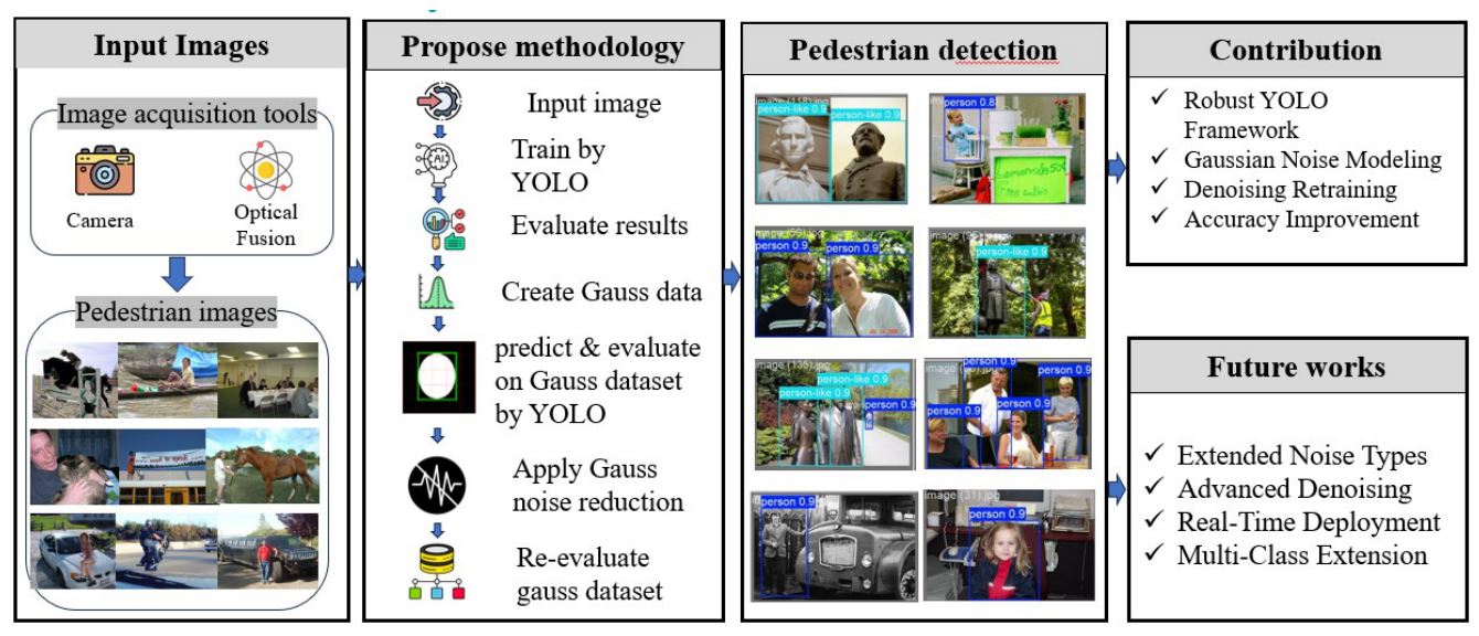
Figure 2.
PnPLO (Person and Person-Like Objects) image datasets.
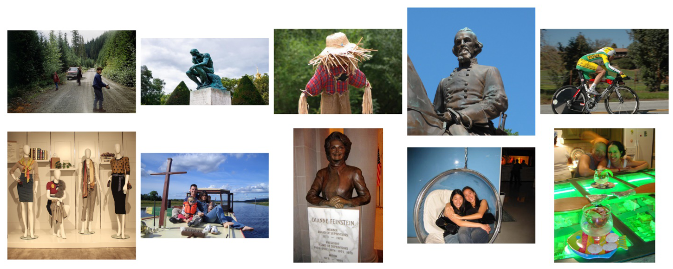
Figure 3.
Training and Validation Performance on Original PnPLO Dataset across YOLO variants (v8m–v12m).
Figure 3.
Training and Validation Performance on Original PnPLO Dataset across YOLO variants (v8m–v12m).
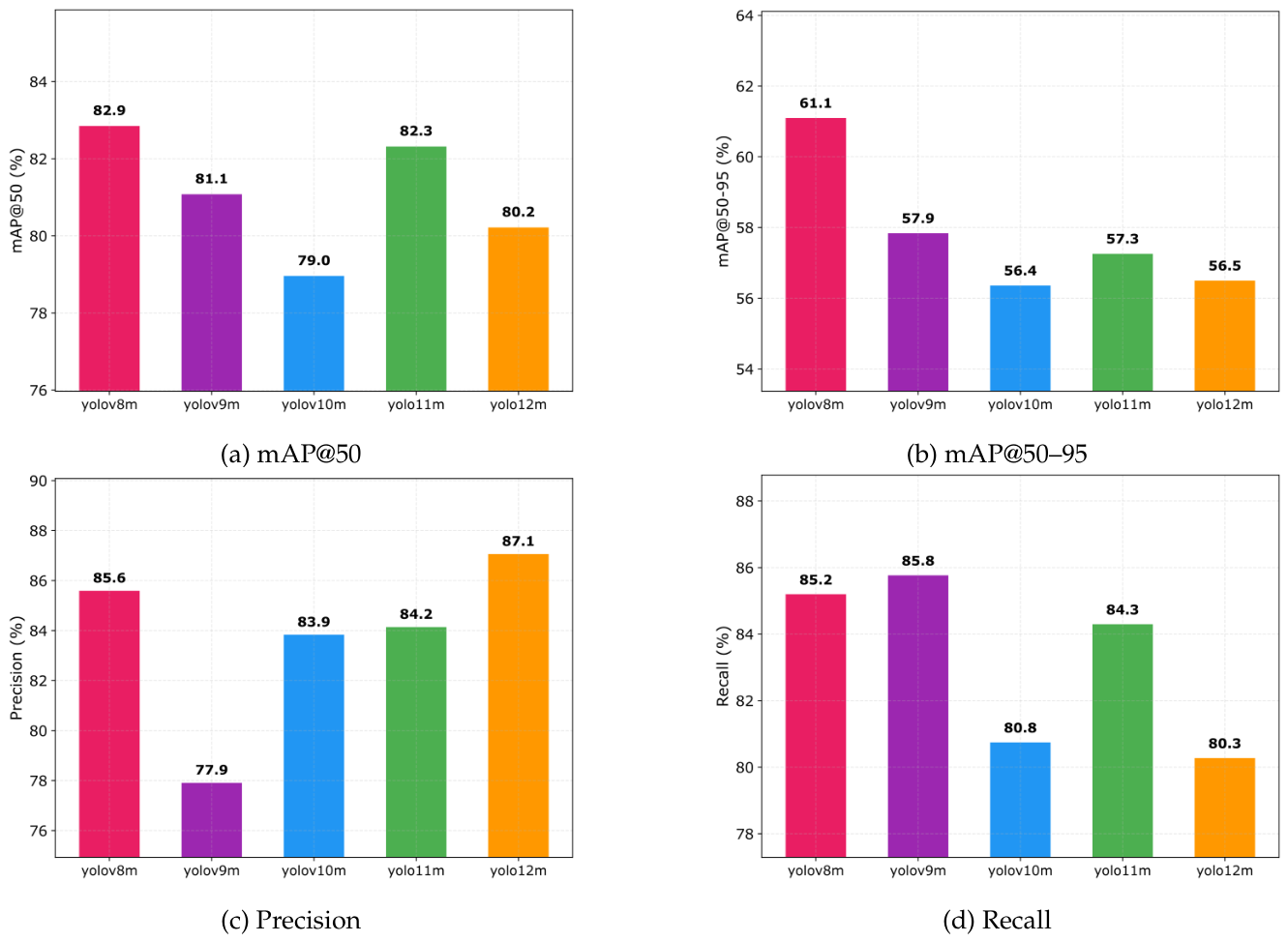
Figure 4.
Heatmap of detection metrics (mAP@50, mAP@50–95, Precision, Recall) on the original (clean) PnPLO dataset.
Figure 4.
Heatmap of detection metrics (mAP@50, mAP@50–95, Precision, Recall) on the original (clean) PnPLO dataset.
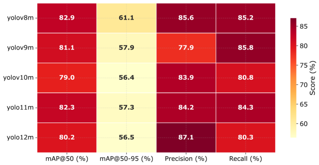
Figure 5.
Object Detection Performance on Original PnPLO Dataset.
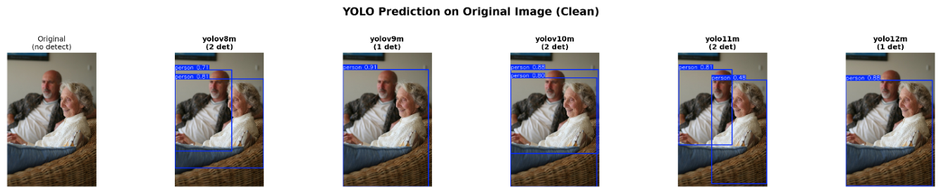
Figure 6.
Detection metrics versus Gaussian noise level for YOLOv8m–YOLOv12m, with no denoising applied.
Figure 6.
Detection metrics versus Gaussian noise level for YOLOv8m–YOLOv12m, with no denoising applied.
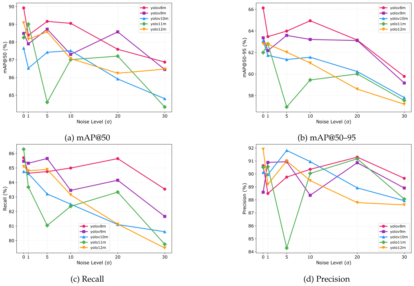
Figure 7.
Heatmap of detection metrics across YOLO variants and Gaussian noise levels under no denoising.
Figure 7.
Heatmap of detection metrics across YOLO variants and Gaussian noise levels under no denoising.
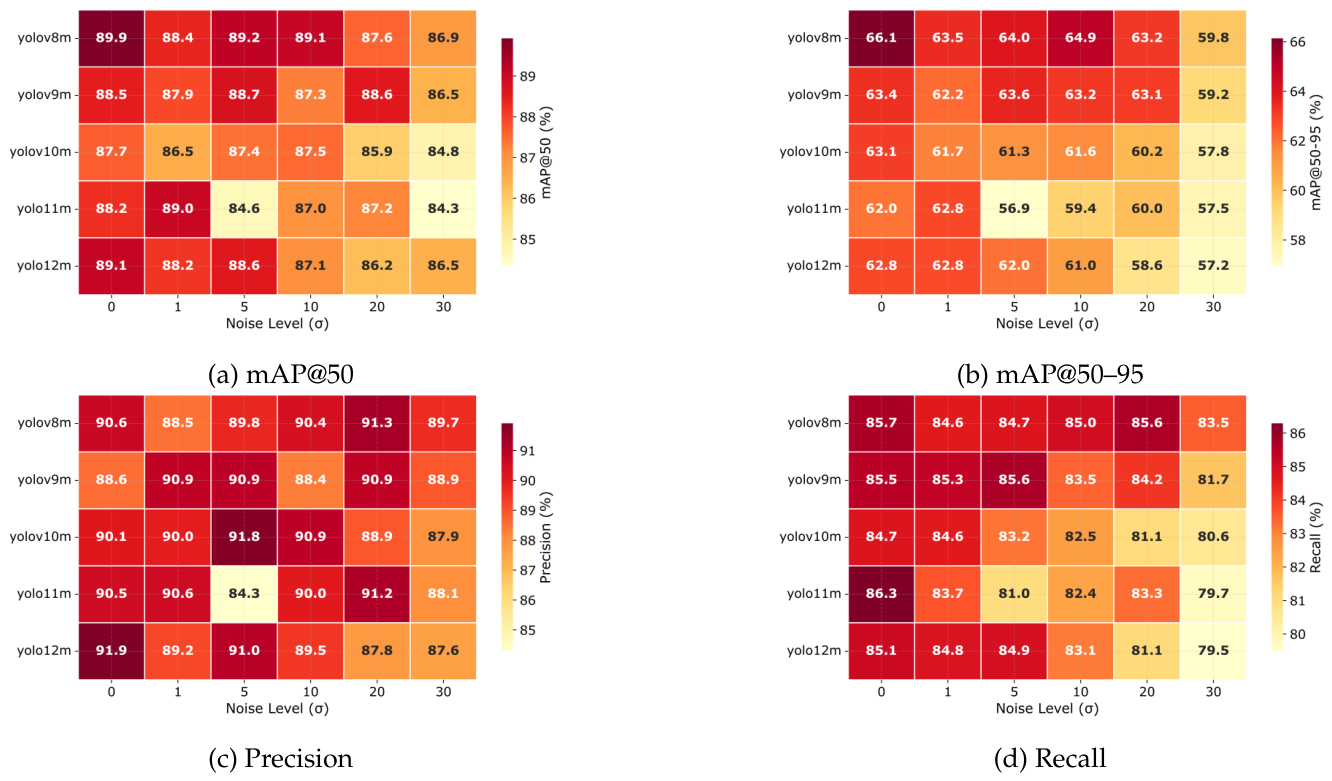
Figure 8.
Object detection performance on Gaussian-noisy images without denoising. Each row corresponds to one YOLO variant; columns show predictions at increasing noise levels.
Figure 8.
Object detection performance on Gaussian-noisy images without denoising. Each row corresponds to one YOLO variant; columns show predictions at increasing noise levels.
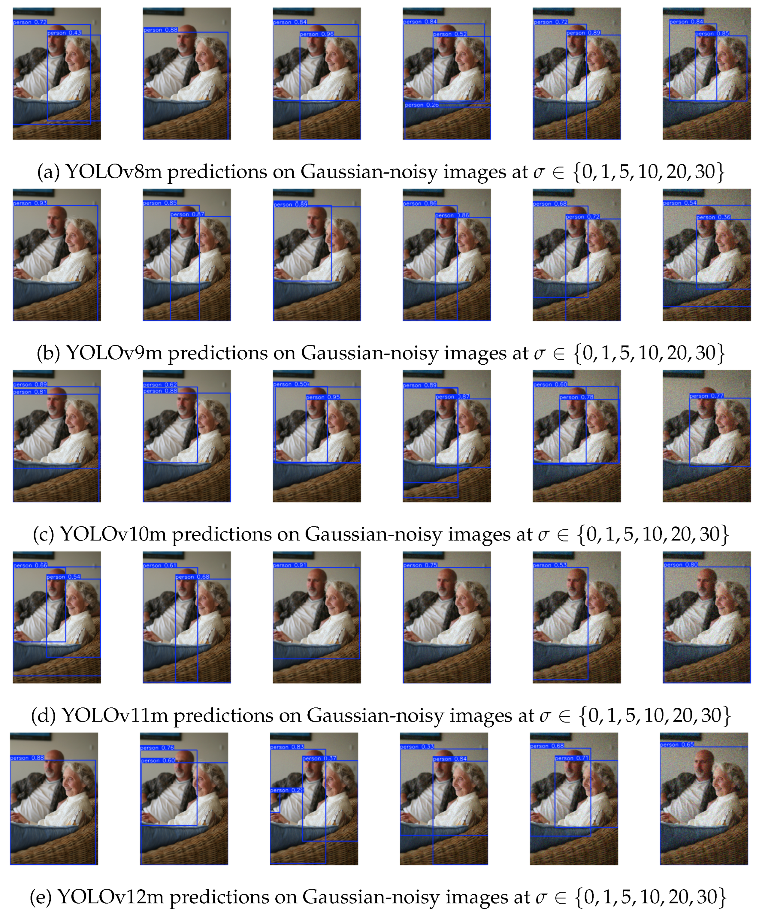
Figure 9.
Detection metrics versus Gaussian noise level after Gaussian-Filter denoising and retraining for YOLOv8m–YOLOv12m.
Figure 9.
Detection metrics versus Gaussian noise level after Gaussian-Filter denoising and retraining for YOLOv8m–YOLOv12m.
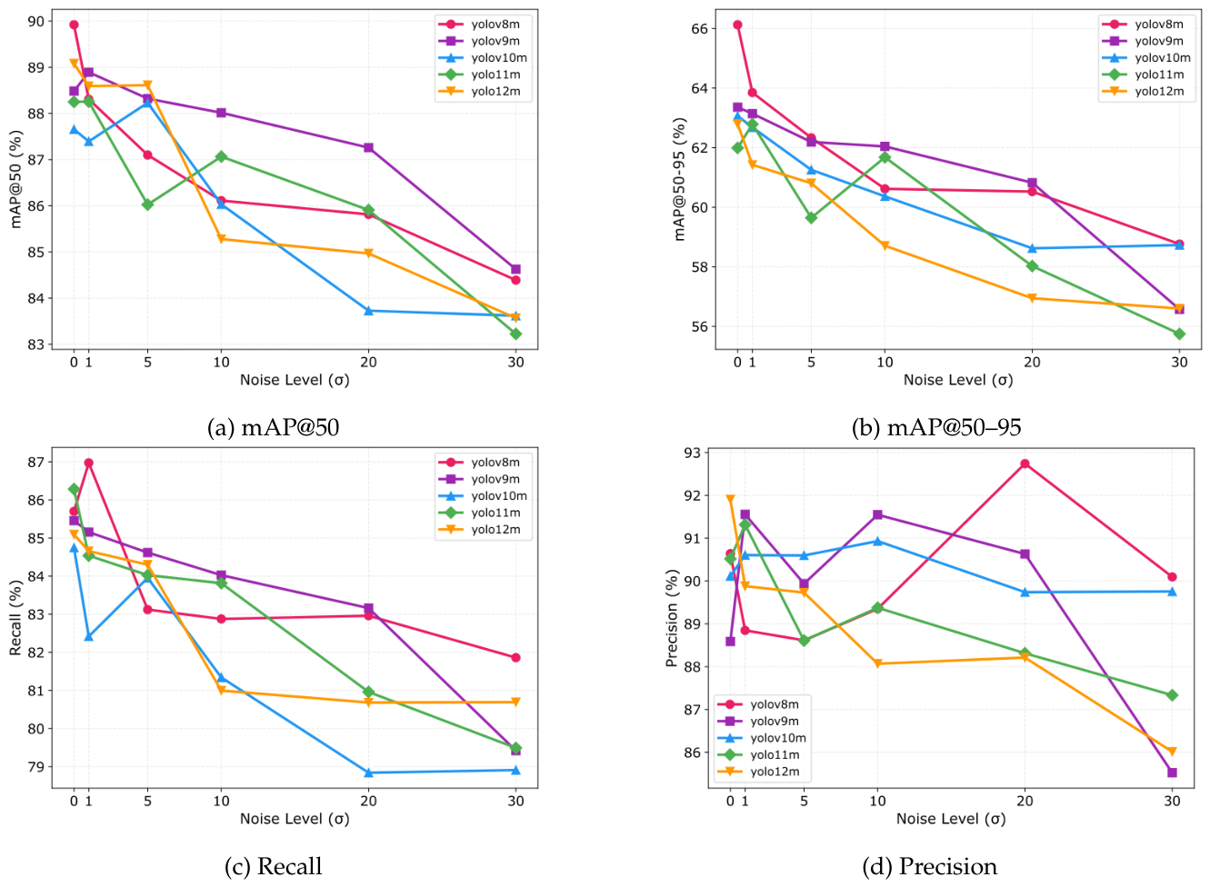
Figure 10.
Heatmap of detection metrics after Gaussian-Filter denoising and retraining across YOLO variants and noise levels.
Figure 10.
Heatmap of detection metrics after Gaussian-Filter denoising and retraining across YOLO variants and noise levels.
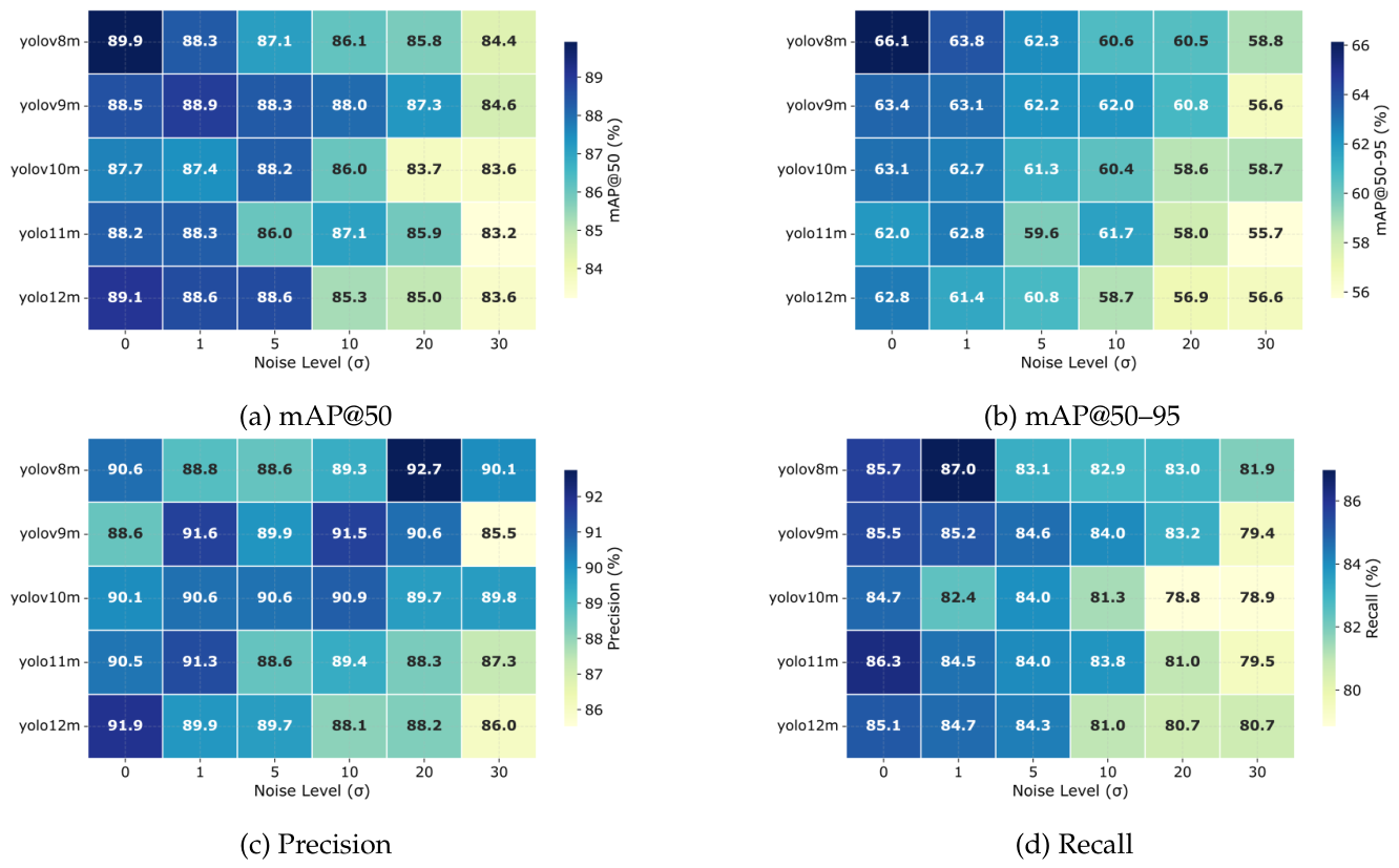
Figure 11.
Object detection performance after denoising.
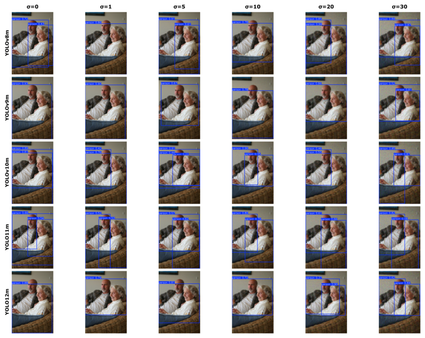
Figure 12.
Effect of six denoising methods on mAP@50 versus Gaussian noise level for each YOLO variant.
Figure 12.
Effect of six denoising methods on mAP@50 versus Gaussian noise level for each YOLO variant.
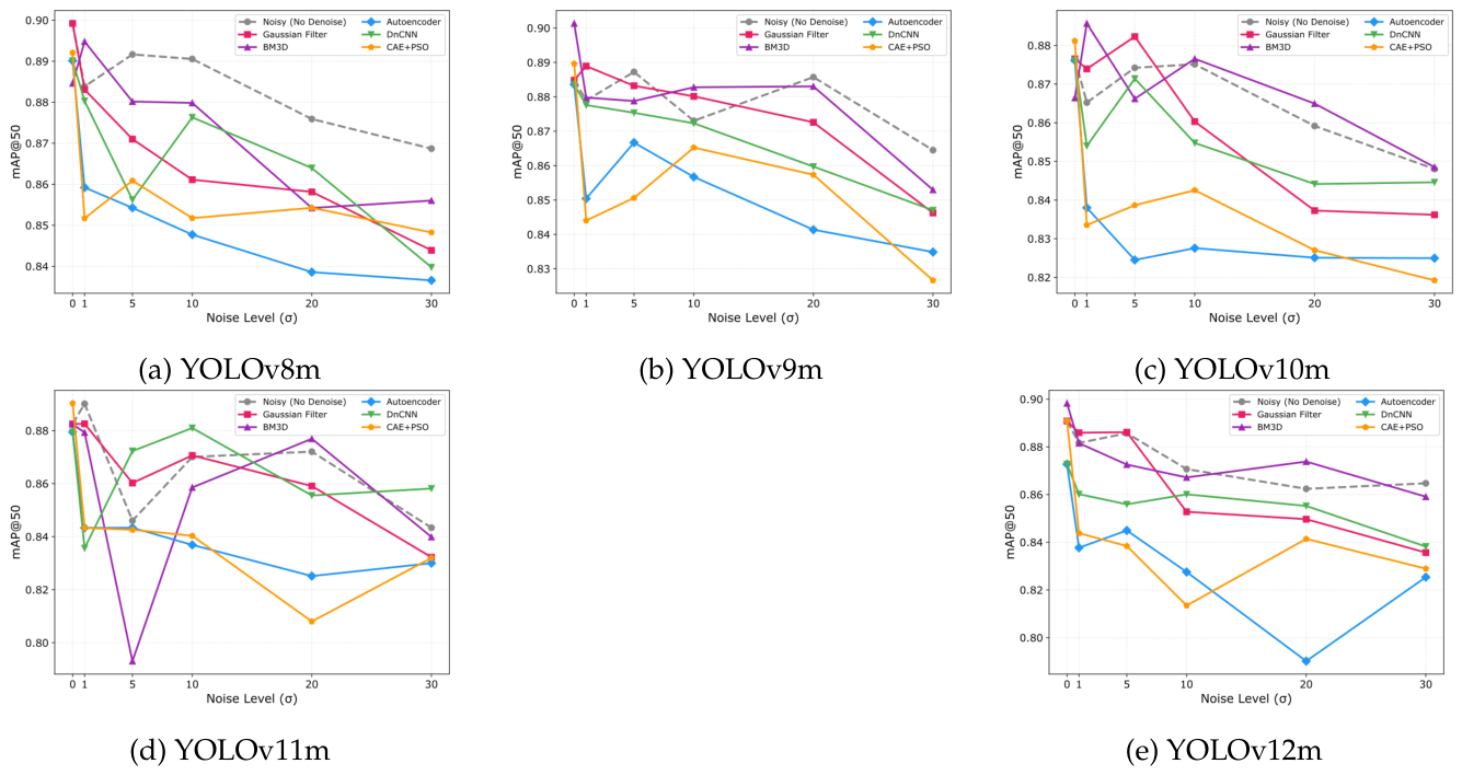
Figure 13.
Heatmap of mAP@50 across YOLO variants and Gaussian noise levels for each of the six denoising strategies.
Figure 13.
Heatmap of mAP@50 across YOLO variants and Gaussian noise levels for each of the six denoising strategies.
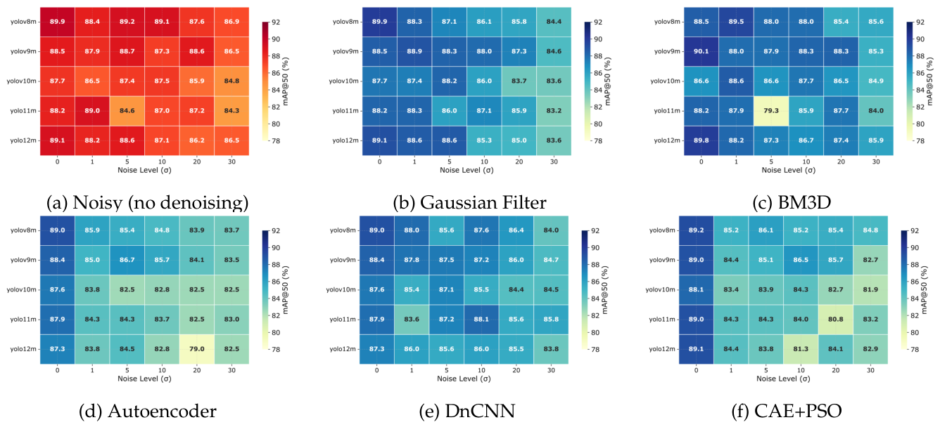
Figure 14.
Aggregate comparison of YOLO variants and denoising methods, averaged across all noise levels.
Figure 14.
Aggregate comparison of YOLO variants and denoising methods, averaged across all noise levels.
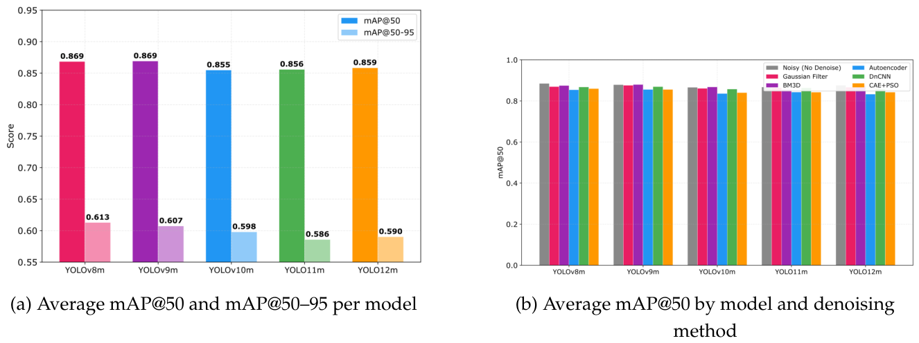
Figure 15.
Denoising effectiveness measured as mAP@50 relative to the noisy baseline, averaged over the noisy levels .
Figure 15.
Denoising effectiveness measured as mAP@50 relative to the noisy baseline, averaged over the noisy levels .
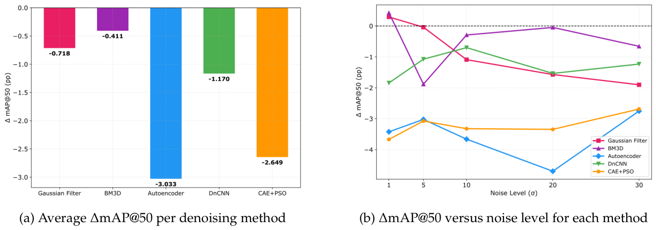
Figure 16.
Object detection performance under each of the six denoising methods at , per YOLO variant.
Figure 16.
Object detection performance under each of the six denoising methods at , per YOLO variant.
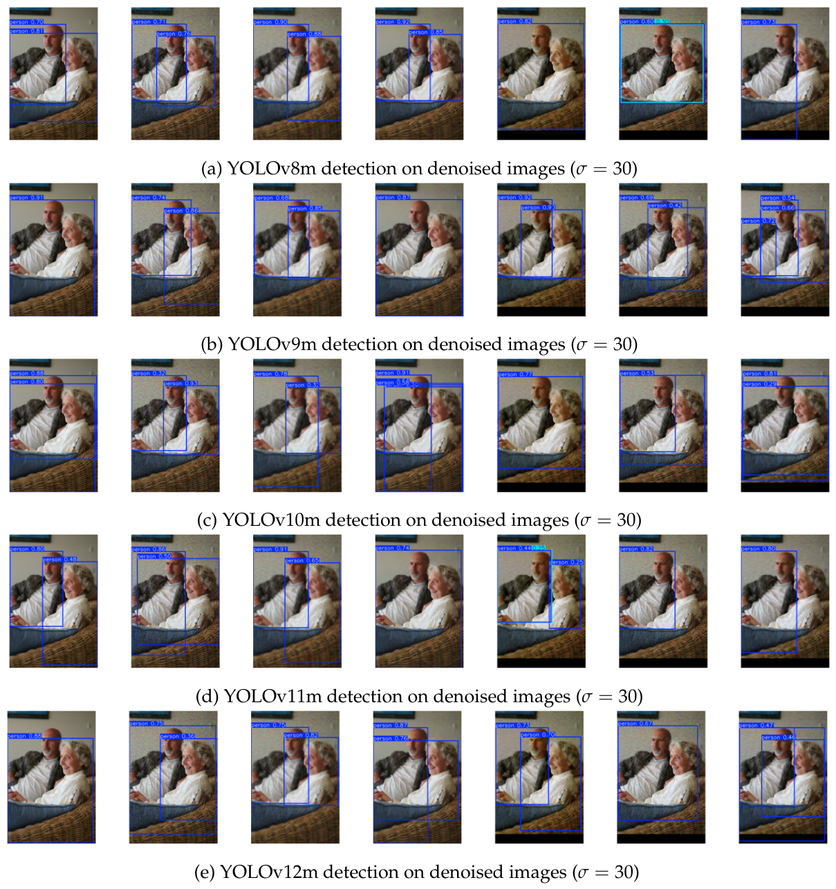
Table 1.
Comparison of recent YOLO benchmark studies and the present study.
| Author, source, year | Algorithm | Dataset | Test condition | Results |
|---|---|---|---|---|
| Jiang & Zhong (2025) [15] | YOLOv5–YOLOv11 | 33 datasets, 11 domains | Clean (multi-domain) | YOLOv11 best in 6 of 11 domains |
| Jegham et al. (2024) [16] | YOLOv3–YOLOv12, YOLO11 | Traffic Signs, African Wildlife, Ships & Vessels | Clean | YOLO11 best accuracy / efficiency balance |
| Sapkota et al. (2025) [17] | YOLOv8–YOLOv12 | Fruitlet (orchard) | Clean | mAP@50 up to 0.935 (YOLOv9 GELAN); 0.933 (YOLO11s); 0.931 (YOLOv12l) |
| Gholinavaz et al. (2025) [18] | YOLOv5s, v8m, v10n, Faster R-CNN | DAWN traffic (1000 images) | Fog, rain, snow, sandstorms; Gaussian / salt-and-pepper noise; blur; haze | mAP@50 = 0.712 (v8m, clean); 0.639 under Gaussian noise |
| Apostolidis et al. (2025) [19] | YOLOv3–v11, YOLOX | MS COCO + corruptions | Adversarial, Gaussian, fog | YOLOv3 / v4 best under Gaussian noise |
| Nabahirwa et al. (2025) [20] | YOLOv8m, v9c, v10m, v11m, v12m | DUO + Roboflow100 (∼10 000 images) | Underwater + noise / blur / colour | YOLOv12 best on clean; highly vulnerable to noise |
| Present study | YOLOv8m–YOLOv12m + 6 denoisers (Gaussian Filter, BM3D, Autoencoder, DnCNN, CAE+PSO, no-denoising baseline) | PnPLO (1339 images) | Gaussian noise + denoising + retraining | mAP@50 = 0.8992 (YOLOv8m, clean); mAP@50 across 6 denoisers |
Table 3.
Performance Comparison of YOLO Models on the Original (Clean) PnPLO Dataset. Accuracy, F1-Score, Sensitivity, Specificity, Precision, and Recall are computed from the confusion matrix produced by post-training validation of each best.pt checkpoint at confidence threshold and IoU threshold , while mAP@50 and mAP@50–95 are reported as the maximum across the 500 training-validation epochs at the default detector threshold. The latter convention is also used for the column of Table 4 to keep cross-noise comparisons consistent.
Table 3.
Performance Comparison of YOLO Models on the Original (Clean) PnPLO Dataset. Accuracy, F1-Score, Sensitivity, Specificity, Precision, and Recall are computed from the confusion matrix produced by post-training validation of each best.pt checkpoint at confidence threshold and IoU threshold , while mAP@50 and mAP@50–95 are reported as the maximum across the 500 training-validation epochs at the default detector threshold. The latter convention is also used for the column of Table 4 to keep cross-noise comparisons consistent.
| Evaluation Items | YOLOv8m | YOLOv9m | YOLOv10m | YOLOv11m | YOLOv12m |
|---|---|---|---|---|---|
| Accuracy | 0.7738 | 0.7812 | 0.7474 | 0.7593 | 0.7649 |
| F1-Score | 0.7909 | 0.7902 | 0.7670 | 0.7753 | 0.7852 |
| Sensitivity | 0.8093 | 0.7826 | 0.7560 | 0.7772 | 0.7871 |
| Specificity | 0.7341 | 0.7796 | 0.7368 | 0.7386 | 0.7381 |
| Precision | 0.8561 | 0.7793 | 0.8399 | 0.8415 | 0.8704 |
| Recall | 0.8521 | 0.8578 | 0.8069 | 0.8448 | 0.8029 |
| mAP50 | 0.8992 | 0.8849 | 0.8766 | 0.8825 | 0.8908 |
| mAP50–95 | 0.6613 | 0.6336 | 0.6306 | 0.6199 | 0.6280 |
Table 4.
Performance Evaluation of YOLO Models under Different Gaussian Noise Levels on PnPLO Dataset.
Table 4.
Performance Evaluation of YOLO Models under Different Gaussian Noise Levels on PnPLO Dataset.
| Metric | YOLOv8m | YOLOv9m | YOLOv10m | YOLOv11m | YOLOv12m | |
|---|---|---|---|---|---|---|
| Accuracy | 0 | 0.7738 | 0.7812 | 0.7474 | 0.7593 | 0.7649 |
| 1 | 0.7920 | 0.7717 | 0.7234 | 0.8000 | 0.7967 | |
| 5 | 0.8028 | 0.7823 | 0.7430 | 0.7132 | 0.7392 | |
| 10 | 0.7892 | 0.7618 | 0.7474 | 0.7677 | 0.7306 | |
| 20 | 0.7874 | 0.7933 | 0.7185 | 0.7608 | 0.7318 | |
| 30 | 0.7586 | 0.7252 | 0.6910 | 0.7442 | 0.7183 | |
| F1-Score | 0 | 0.7909 | 0.7902 | 0.7670 | 0.7753 | 0.7852 |
| 1 | 0.8098 | 0.7862 | 0.7194 | 0.8146 | 0.8114 | |
| 5 | 0.8325 | 0.7990 | 0.7488 | 0.7447 | 0.7517 | |
| 10 | 0.7969 | 0.7673 | 0.7557 | 0.7689 | 0.7360 | |
| 20 | 0.8083 | 0.8077 | 0.7382 | 0.7747 | 0.7361 | |
| 30 | 0.7688 | 0.7465 | 0.7040 | 0.7537 | 0.7268 | |
| Precision | 0 | 0.9064 | 0.8859 | 0.9011 | 0.9052 | 0.9190 |
| 1 | 0.8849 | 0.9089 | 0.8995 | 0.9056 | 0.8919 | |
| 5 | 0.8975 | 0.9094 | 0.9181 | 0.8429 | 0.9101 | |
| 10 | 0.9036 | 0.8835 | 0.9095 | 0.9004 | 0.8949 | |
| 20 | 0.9130 | 0.9087 | 0.8892 | 0.9117 | 0.8779 | |
| 30 | 0.8996 | 0.8891 | 0.8794 | 0.8806 | 0.8761 | |
| Recall | 0 | 0.8570 | 0.8546 | 0.8475 | 0.8629 | 0.8510 |
| 1 | 0.8463 | 0.8532 | 0.8461 | 0.8368 | 0.8481 | |
| 5 | 0.8475 | 0.8565 | 0.8321 | 0.8103 | 0.8489 | |
| 10 | 0.8499 | 0.8345 | 0.8250 | 0.8235 | 0.8315 | |
| 20 | 0.8564 | 0.8415 | 0.8110 | 0.8333 | 0.8113 | |
| 30 | 0.8313 | 0.8166 | 0.8061 | 0.7974 | 0.7948 | |
| mAP50 | 0 | 0.8992 | 0.8849 | 0.8766 | 0.8825 | 0.8908 |
| 1 | 0.8839 | 0.8790 | 0.8652 | 0.8901 | 0.8817 | |
| 5 | 0.8917 | 0.8873 | 0.8742 | 0.8460 | 0.8857 | |
| 10 | 0.8905 | 0.8730 | 0.8751 | 0.8701 | 0.8707 | |
| 20 | 0.8759 | 0.8857 | 0.8592 | 0.8721 | 0.8624 | |
| 30 | 0.8682 | 0.8645 | 0.8480 | 0.8434 | 0.8647 | |
| mAP50–95 | 0 | 0.6613 | 0.6336 | 0.6306 | 0.6199 | 0.6280 |
| 1 | 0.6347 | 0.6217 | 0.6173 | 0.6280 | 0.6276 | |
| 5 | 0.6398 | 0.6358 | 0.6134 | 0.5694 | 0.6202 | |
| 10 | 0.6494 | 0.6321 | 0.6156 | 0.5945 | 0.6102 | |
| 20 | 0.6315 | 0.6311 | 0.6023 | 0.6001 | 0.5860 | |
| 30 | 0.5978 | 0.5917 | 0.5781 | 0.5754 | 0.5719 |
Table 5.
Training and Validation Performance Curves for YOLO Variant Comparison after Denoising.
| Metric | YOLOv8m | YOLOv9m | YOLOv10m | YOLOv11m | YOLOv12m | |
|---|---|---|---|---|---|---|
| Accuracy | 0 | 0.7738 | 0.7812 | 0.7474 | 0.7593 | 0.7649 |
| 1 | 0.7875 | 0.7932 | 0.7450 | 0.7814 | 0.7679 | |
| 5 | 0.7507 | 0.7613 | 0.7388 | 0.7730 | 0.7834 | |
| 10 | 0.7550 | 0.7704 | 0.7637 | 0.7742 | 0.7554 | |
| 20 | 0.7634 | 0.7696 | 0.7047 | 0.7468 | 0.7302 | |
| 30 | 0.7388 | 0.7228 | 0.7291 | 0.7016 | 0.7209 | |
| F1-Score | 0 | 0.7909 | 0.7902 | 0.7670 | 0.7753 | 0.7852 |
| 1 | 0.8060 | 0.8030 | 0.7619 | 0.7970 | 0.7797 | |
| 5 | 0.7579 | 0.7775 | 0.7531 | 0.7812 | 0.8010 | |
| 10 | 0.7772 | 0.7809 | 0.7795 | 0.7868 | 0.7661 | |
| 20 | 0.7742 | 0.7833 | 0.7187 | 0.7519 | 0.7335 | |
| 30 | 0.7531 | 0.7358 | 0.7432 | 0.7000 | 0.7353 | |
| Precision | 0 | 0.9064 | 0.8859 | 0.9011 | 0.9052 | 0.9190 |
| 1 | 0.8885 | 0.9156 | 0.9060 | 0.9131 | 0.8988 | |
| 5 | 0.8861 | 0.8994 | 0.9060 | 0.8861 | 0.8973 | |
| 10 | 0.8935 | 0.9155 | 0.9093 | 0.8937 | 0.8807 | |
| 20 | 0.9274 | 0.9063 | 0.8974 | 0.8831 | 0.8821 | |
| 30 | 0.9010 | 0.8552 | 0.8976 | 0.8733 | 0.8601 | |
| Recall | 0 | 0.8570 | 0.8546 | 0.8475 | 0.8629 | 0.8510 |
| 1 | 0.8697 | 0.8516 | 0.8242 | 0.8454 | 0.8466 | |
| 5 | 0.8312 | 0.8462 | 0.8395 | 0.8403 | 0.8430 | |
| 10 | 0.8288 | 0.8403 | 0.8134 | 0.8382 | 0.8100 | |
| 20 | 0.8296 | 0.8316 | 0.7884 | 0.8096 | 0.8068 | |
| 30 | 0.8186 | 0.7942 | 0.7891 | 0.7949 | 0.8069 | |
| mAP50 | 0 | 0.8992 | 0.8849 | 0.8766 | 0.8825 | 0.8908 |
| 1 | 0.8831 | 0.8889 | 0.8739 | 0.8826 | 0.8859 | |
| 5 | 0.8710 | 0.8832 | 0.8823 | 0.8602 | 0.8861 | |
| 10 | 0.8611 | 0.8801 | 0.8603 | 0.8706 | 0.8528 | |
| 20 | 0.8581 | 0.8726 | 0.8373 | 0.8591 | 0.8497 | |
| 30 | 0.8439 | 0.8463 | 0.8362 | 0.8322 | 0.8357 | |
| mAP50–95 | 0 | 0.6613 | 0.6336 | 0.6306 | 0.6199 | 0.6280 |
| 1 | 0.6385 | 0.6314 | 0.6268 | 0.6279 | 0.6142 | |
| 5 | 0.6233 | 0.6219 | 0.6125 | 0.5964 | 0.6080 | |
| 10 | 0.6062 | 0.6204 | 0.6036 | 0.6168 | 0.5871 | |
| 20 | 0.6052 | 0.6082 | 0.5862 | 0.5802 | 0.5694 | |
| 30 | 0.5876 | 0.5657 | 0.5873 | 0.5574 | 0.5660 |
Disclaimer/Publisher’s Note: The statements, opinions and data contained in all publications are solely those of the individual author(s) and contributor(s) and not of MDPI and/or the editor(s). MDPI and/or the editor(s) disclaim responsibility for any injury to people or property resulting from any ideas, methods, instructions or products referred to in the content. |
© 2026 by the authors. Licensee MDPI, Basel, Switzerland. This article is an open access article distributed under the terms and conditions of the Creative Commons Attribution (CC BY) license (http://creativecommons.org/licenses/by/4.0/).
Copyright: This open access article is published under a Creative Commons CC BY 4.0 license, which permit the free download, distribution, and reuse, provided that the author and preprint are cited in any reuse.


