

Submitted:
02 July 2026
Posted:
03 July 2026
You are already at the latest version
Abstract
Operational satellite monitoring of pasture biomass demands models that extrapolate beyond the range of properties on which they were calibrated. We show that the dominant failure mode of Sentinel-2 pasture-biomass models in tropical Australian rangelands is the saturation and phenological inversion of greenness-based vegetation indices across sites, and that this failure can be substantially repaired with open climate and topsoil covariates from public archives. The work builds on a hierarchical pipeline that scales clip-and-weigh ground truth (n=1120 tare-corrected samples across eleven sites on five Queensland properties) through UAV digital-surface-model imagery to Sentinel-2 predictions, using TabPFN – a pre-trained transformer foundation model for small tabular data – as the regressor at all three nested spatial scales, and a seven-class deep-learning pasture mask (overall accuracy 98.6 %) to suppress mixed-pixel noise. Under a leave-one-site-out (LOSO) cross-validation protocol on twenty site-date aggregates across nine sites, spectral-only models failed to transfer across sites (R2=−0.21, RMSE=4.79 t ha-1). Appending open climate (Open-Meteo ERA5) and soil (SoilGrids 2.0) covariates, and switching to a gradient-boosted regressor on log-transformed biomass, lifted LOSO R2 to +0.07 and reduced RMSE to 4.19 t ha-1. A leaf-nitrogen growth trajectory, predicted by the TabPFN nitrogen regressor developed in our earlier pasture chemistry work, reduced LOSO error by a further 11 % relative to greenness-only growth features. Three additional covariate classes – BARRA-R2 reanalysis climate, three independent fractional-cover products, and Sentinel-1 C-band SAR backscatter – were tested and rejected, all hitting the same RMSE floor. The symmetric negative results suggest that the residual LOSO ceiling at the current nine-property footprint is a sample-size and sensor-saturation limit rather than a feature-engineering one, and that the most tractable operational path forward is to stratify the production model by climatic zone and Queensland Land Type rather than pursue further covariates within a single global learner. Expanding UAV calibration footprints and integrating open climate, soil and plant-chemistry data are complementary, not competing, investments for operational rangeland remote sensing.
Keywords:
pasture biomass
; TabPFN
; transformer
; foundation model
; UAV
; digital surface model
; Sentinel-2
; random forest
; time-series
; rangeland monitoring
; hierarchical scaling
; Australia
1. Introduction
Northern Australian rangelands cover more than 4 million km2 and underpin a beef industry of national strategic importance, yet pasture biomass – the single most important variable for matching stocking rates to feed availability – remains poorly quantified at the spatial and temporal resolution needed for tactical grazing decisions [1,2,3]. Standing dry matter (kg DM ha-1) drives carrying capacity, ground-cover thresholds, fire risk, methane emissions and woody-grass competition; under climate variability, accurate near-real-time biomass estimates are central to climate-smart livestock production [4,5].
Conventional measurement of standing biomass relies on destructive clip-and-weigh quadrat sampling, which is accurate at the point but spatially impoverished and labour-intensive. Optical satellite remote sensing has been pursued as a scalable alternative for over three decades; the launch of Sentinel-2 in 2015 transformed the operational outlook by delivering 10 m, 5–10 day revisit and 13-band visible–short-wave infrared coverage [6,7,8,9]. Reported R2 values on Sentinel-2 grassland biomass models range from 0.50 to 0.85, with random-forest and gradient-boosting regressors dominating the recent literature [7,9,10,11]. A common limitation in published cross-validation is reliance on within-site k-fold splits that overstate transferability; leave-one-site-out (LOSO) performance is rarely reported and typically much lower [12].
UAV photogrammetry has emerged as a critical intermediate scale: dense 3-D canopy-height models (CHMs) at sub-decimetre resolution can be related directly to biomass density through canopy-height summary statistics or canopy-relative-height-model metrics [13,14,15,16,17,18]. Reported R2 values for UAV CHM-to-biomass on grasslands span 0.60–0.90, generally higher than satellite-only models because the height signal is mechanistically related to standing biomass and is less affected by soil-background and substrate effects on satellite spectral indices. UAV models, however, are bounded by the tile footprint and require costly repeat flights for time-series, in contrast to the more than 106 km2 extent at which Sentinel-2 monitoring is operationally relevant for Australian rangelands.
Hierarchical scaling protocols that bridge the gap between in situ samples, UAV tiles and continental-scale satellite imagery have been developed for forest biomass [19,20] and increasingly for pasture [21,22]. A typical protocol (i) trains a fine spatial-scale model on in situ samples and a moderate spatial-scale sensor (UAV); (ii) uses the fine-scale model to generate dense “virtual” samples across tile footprints; and (iii) regresses the virtual samples against contemporaneous coarser spatial-scale (Sentinel-2) reflectance to train an operational continental-scale model. The success of this cascade rests on three technical pillars: (a) ground-truth quality and bias correction, (b) the predictive flexibility of the fine-scale and coarse-scale models on small samples, and (c) a robust pasture/non-pasture mask to suppress mixed-pixel noise.
For (b), recent advances in foundation models for tabular data have created a step-change in small-sample regression. TabPFN [23,24] is a pre-trained Bayesian-style transformer that performs in-context learning on tabular inputs, eliminating per-task hyperparameter tuning and outperforming gradient-boosting baselines on datasets with n ≤ 104. TabPFN has rapidly entered agricultural and Earth-observation applications, including continental maize-yield mapping [25], field-scale digital soil mapping [26], and pasture nutritive-composition retrieval [22,27]. To our knowledge, TabPFN has not previously been deployed at three nested spatial scales for the same agroecological target, nor coupled with a random-forest surrogate to enable wall-to-wall raster inference at sub-metre resolution.
This paper presents a complete, open-source, multi-scale TabPFN biomass pipeline that builds on, and extends, the Barnetson et al. [22] pasture nutrition framework. Specifically we (i) re-derive a tare-corrected ground-truth dataset of 1120 dual-geometry quadrat-and-mower samples across 11 sites on five commercial cattle-grazing properties in Queensland; (ii) train a TabPFN UAV digital-surface-model regressor and a random-forest surrogate that delivers 5 cm wall-to-wall biomass rasters across 12 site-dates; (iii) train three Sentinel-2 TabPFN biomass models – snapshot, NDVI-growth, and combined NDVI plus leaf-nitrogen growth – on 856 cloud-free pairs; (iv) demonstrate operational time-series biomass retrieval at 5–10 day cadence on a managed C4 grassland and a grassy-woodland savanna site; and (v) make all code, trained models and per-pixel predictions available on request, subject to the commercial-in-confidence and landholder-privacy terms attached to the underlying fieldwork. The choice of NDVI over a soil-adjusted index such as EVI for the time-series feature stack is justified in Section 2.6; in brief, it preserves continuity with the regional Queensland pasture growth-curve literature [28], and the per-pixel TN trajectory of Stage 3 carries the soil-background-aware information that an EVI-style correction would otherwise add. The contribution is both methodological (TabPFN at three nested scales, with a leaf-N growth trajectory as a biomass feature) and operational (a reproducible time-series for grazing management).
2. Materials and Methods
2.1. Study Area
Five cattle-grazing properties were chosen for this case study, located within the Desert Uplands, Brigalow Belt, and Southeast Queensland bioregions. All five properties were located within the Great Barrier Reef (GBR) catchment of Queensland, Australia. Grazing (77%) is the dominant agricultural land use of the GBR [29] and contributes to increased levels of sediments and nutrients. Improved grazing land management practices contribute to reduced sedimentation and nutrient deposition.
The climate of the study area is predominantly hot, humid summer zone for Property A (Baralaba region) and warm, humid summer zone for the more northerly and westerly properties (B, C, D). Property E is located in a subtropical climate zone in southeast Queensland. Each field site was chosen to represent the main productive vegetation groups of each property. Field sites were sampled up to five times during 2023–2025, capturing late wet (April–May 2023), dry (August–November 2023), wet (January–April 2024), dry (August–October 2024), and a further dry-season revisit (May–September 2025) at a subset of sites (boundary, trafAlt, mtp01, bonna01, bary01, esk01) to assess temporal variability in pasture biomass.
Figure 1.
Field-site locations and representative ground-level photographs. Top: field-site locations across Great Barrier Reef catchments and bioregions in Queensland, Australia (Properties A–E); reference cities (Brisbane, Rockhampton, Townsville) shown for context. Base-map vector layers (land, ocean, coastline, rivers, state boundaries) are drawn from Natural Earth 1:10m physical and cultural data (https://www.naturalearthdata.com/) via the Cartopy Python package [30]. Bottom: representative ground-level photographs at each of the nine field sites (a)–(i), taken in landscape orientation looking across the dominant pasture sward at the time of a representative UAV flight. The nine sites span the productive vegetation groups summarised in Table 1: open native/naturalised C4 grassland (boundary, bonna01, bary01, esk01), mixed grass/woody pastures (appletree, bonna02, bary02) and grassy eucalypt woodland (mtp01, mtp02). The visual range from short-grazed grassland to tall tussock biomass under partial overstory is the structural and phenological diversity that the cross-site LOSO benchmark (Section 3.3) probes.
Figure 1.
Field-site locations and representative ground-level photographs. Top: field-site locations across Great Barrier Reef catchments and bioregions in Queensland, Australia (Properties A–E); reference cities (Brisbane, Rockhampton, Townsville) shown for context. Base-map vector layers (land, ocean, coastline, rivers, state boundaries) are drawn from Natural Earth 1:10m physical and cultural data (https://www.naturalearthdata.com/) via the Cartopy Python package [30]. Bottom: representative ground-level photographs at each of the nine field sites (a)–(i), taken in landscape orientation looking across the dominant pasture sward at the time of a representative UAV flight. The nine sites span the productive vegetation groups summarised in Table 1: open native/naturalised C4 grassland (boundary, bonna01, bary01, esk01), mixed grass/woody pastures (appletree, bonna02, bary02) and grassy eucalypt woodland (mtp01, mtp02). The visual range from short-grazed grassland to tall tussock biomass under partial overstory is the structural and phenological diversity that the cross-site LOSO benchmark (Section 3.3) probes.
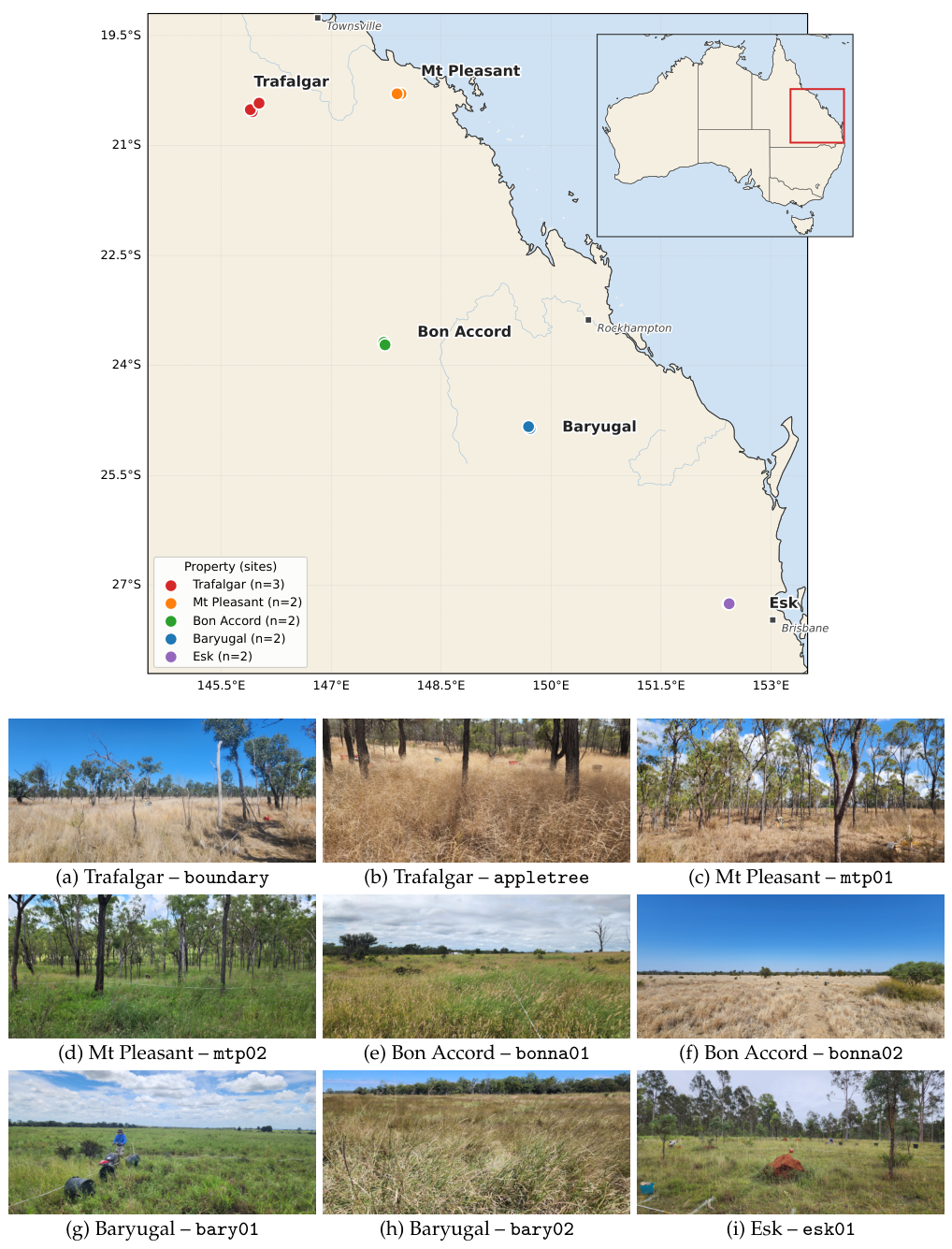
Table 1 details the dominant vegetation groups sampled across each property and field site.
Table A1 details the sampling schedule for each field site, including coordinates and visit dates; the full site-list table is reported in Appendix A.
2.2. Field Sampling and Tare Correction
Two complementary destructive sampling geometries were used at every site–date.
Quadrat clips. 0.5 m × 0.5 m frame, 0.25 m2 sampling area. All standing biomass within the frame was clipped to an approximate stubble height of 5 cm above the soil surface (Figure 2a,b), consistent with conventional pasture standing-biomass estimation that excludes the basal crown and root mat. Cut material was sealed in a numbered brown paper bag (mass 43.45 g, =0.6 g, n=20 calibration weighings), oven-dried at 70°C for 48 h, and weighed.
Mower swaths. A pedestrian-pushed reciprocating mower harvested all standing biomass within a polygon-defined area (1–4 m2 per swath, GNSS-mapped) at a comparable cutting height of ∼5 cm. Material was sealed in a green PVC catch-bag (mass 360 g, =4.1 g, n=12 calibration weighings) and weighed wet in the field. Mower swaths were not oven-dried because of the prohibitive logistics of transporting and drying the high-volume catch-bag samples from remote sites; dry weights were instead reconstructed by applying the wet-to-dry moisture factor measured for the spatially nearest oven-dried quadrat at the same site–date to each mower wet mass. The three field stages of mower sampling are illustrated in Figure 2.
Bag-tare correction is applied per geometry before density conversion:
The tare-corrected dataset comprises 1120 samples (489 q, 631 m) across 11 sites on 5 commercial properties. Applying the tare correction uniformly to all 1120 samples lowered the population-mean dry-biomass density from 4.61 to 3.30 t ha-1 (−1.31 t ha-1), driven predominantly by the 360 g mower-bag tare; within-site variance was largely preserved ( 2.91 → 2.82 t ha-1), so the correction acts as a bias offset rather than a rescaling of the biomass distribution.
2.3. UAV Acquisition and DSM Canopy-Height Model
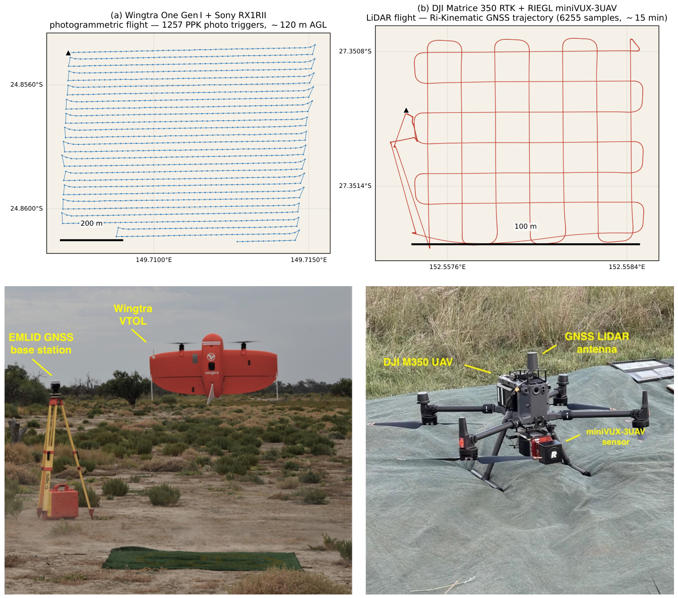
Two complementary UAV platforms were used to derive the digital surface models (DSMs), matching the acquisition strategy of the companion pasture chemistry study [22]. For 2023 and 2024 site-dates, photogrammetric flights used a Wingtra One Gen I fixed-wing VTOL platform with a 42 MP Sony RX1RII full-frame RGB camera (PPK-corrected GNSS, 100–120 m AGL, 80%/70% overlap), processed in Pix4Dmapper to a 3–5 cm orthomosaic and a 5 cm DSM. For 2025 acquisitions, a RIEGL miniVUX-3UAV survey-grade LiDAR sensor mounted on a DJI Matrice 350 RTK multi-rotor was flown at 60–80 m AGL with 50–80 points m-2, decoded in RIEGL RiPROCESS with trajectory fusion and PPK georeferencing performed in Ri-Kinematic. Direct georeferencing for both platforms used PPK GNSS with an Emlid RS2 base station deployed at each site, achieving sub-decimetre positional accuracy. Representative flight patterns and platform photographs are shown in Appendix B, Figure A1.
For both modalities a bare-earth DTM was generated by cloth-simulation filtering of the dense point cloud, and a 5 cm CHM derived as . Mean horizontal absolute positional accuracy assessed against four ground control points was 4.1 cm (Wingtra) and 2.8 cm (miniVUX). CHM pixels were intersected with each ODK quadrat or mower polygon and per-polygon height summary statistics (mean, median, P95, max, standard deviation) extracted. The two DSM sources were pooled in the training set; an indicator covariate (dsm_source) was retained but made no significant contribution to TabPFN cross-validation scores (), confirming that height is a sensor-agnostic descriptor at the polygon scale. A faint orthogonal banding visible at the photo-footprint scale (∼10–20 m) in some photogrammetric CHMs is a residual block-bundle-adjustment / cloth-simulation artefact, most apparent over timbered areas; it averages out at the polygon scale used to train the biomass model and is left visible in Figure 3 for transparency.
2.4. UAV Biomass Model: TabPFN Regressor with Random-Forest Surrogate
Polygon-aggregated CHM statistics for q+m geometries were pooled (n=489 polygons across 12 site-dates) and used to train a single TabPFN regressor predicting tare-corrected dry biomass density (g m-2). Five height predictors (mean_height_m, median_height_m, p95_height_m, max_height_m, std_height_m) were standardised (mean 0, sd 1) using site-pooled training statistics. TabPFN v2 was used in CPU mode with 32 ensemble members; no hyperparameter tuning was performed (TabPFN is parameter-free at inference).
For wall-to-wall raster inference (108 pixels per tile, infeasible for direct TabPFN inference at ∼1 ms/sample), a random-forest surrogate (n_estimators=500, max_depth=12, min_samples_leaf=20) was fitted to TabPFN training-set predictions and applied tile-by-tile to each site’s CHM raster. Surrogate fidelity, assessed on a held-out 20% in-sample set, was R2=0.97 and RMSE=0.34 t ha-1, well within ground-truth measurement noise.
Validation used three nested cross-validation schemes: (i) in-sample, (ii) 5-fold stratified by (site, date), and (iii) leave-one-site-out (LOSO).
2.5. Pasture Classification Mask
Wall-to-wall biomass rasters were masked to “productive pasture” pixels using the deep-learning land-cover classifier described in [22] (7 classes – bare, dead-pasture, green-pasture, mixed-pasture, woody, water, infrastructure – with overall accuracy 98.6%). All pasture-class pixels (green-pasture, dead-pasture and mixed-pasture) were retained; site-dates lacking a contiguous pasture-class polygon were excluded from Sentinel-2 training pair extraction (Table A1).
2.6. Sentinel-2 Training Pair Extraction and Modelling Pipeline
The Sentinel-2 biomass modelling pipeline comprises three stages of increasing temporal context, each built on the same set of cloud-free UAV/Sentinel-2 training pairs:
- Stage 1 – Snapshot model: 10 surface-reflectance bands (B02 blue, B03 green, B04 red, B05 red-edge 1, B06 red-edge 2, B07 red-edge 3, B08 near-infrared, B8A near-infrared narrow, B11 short-wave-infrared 1, B12 short-wave-infrared 2) from the cloud-free Sentinel-2 scene closest to each UAV acquisition.
- Stage 2 – NDVI-growth model: 8 derived NDVI time-series features from the 12 months preceding each UAV date. NDVI was retained (over soil-adjusted alternatives such as EVI) because it provides the longest gap-free archival record for regional Queensland-pasture growth-curve work [28] and because the soil-background-aware information that EVI would add is already carried by the per-pixel TN trajectory introduced in Stage 3; the well-known NDVI saturation above ∼2–3 t ha-1 [31,32] is the same effect we exploit in Section 3.3 to explain why fractional-cover and SAR covariates fail to lift cross-site performance.
- Stage 3 – NDVI + TN-growth model: the 8 NDVI-growth features plus 8 total-nitrogen (TN) growth features (16 in total) over the same 12-month window.
Sentinel-2 L2A scenes were queried via the Element 84 Earth-Search STAC API (https://earth-search.aws.element84.com/v1, public Cloud-Optimized GeoTIFF access). For each masked UAV biomass raster (), all scenes within ±5 d of with >5 % clear pixels were retained, where clear pixels are Sen2Cor Scene Classification Layer (SCL) classes 4 (vegetation), 5 (bare soils), 6 (water) and 7 (unclassified), excluding all cloud, cloud-shadow and saturated/defective categories. The ten reflectance bands (10 m natives B02/B03/B04/B08; 20 m natives B05/B06/B07/B8A/B11/B12 bilinearly resampled) and the pasture-masked biomass labels were aggregated to a common 10 m grid covering the UAV footprint, yielding 856 cloud-free 10 m Stage 1 (snapshot) training pairs.
For Stages 2 and 3 we extended the search window to the 12 months preceding each and extracted, per pixel, the per-scene NDVI trajectory and—for Stage 3—a per-pixel total-nitrogen (TN, % dry weight) trajectory using the TabPFN nitrogen regressor of [22] (n=369 train + 93 val, val R2=0.916, RMSE=0.063 % TN). Following the satellite-time-series growth-curve approach of [28], eight derived features were engineered per trajectory: value at , time-integral, mean and peak growth-window value, persistence (fraction of scenes above the 70th percentile), days from peak to , growth-window length, and number of clear observations. Pairs with fewer than 5 clear scenes in the window were discarded, leaving 641 Stage 2 and 500 Stage 3 pairs; the additional Stage 3 attrition arises because the TN regressor masks scenes whose 10-band reflectance lies outside its green-canopy training envelope (predominantly winter/senescent or sub-pixel-haze acquisitions).
2.7. Sentinel-2 Biomass Models
All three Sentinel-2 models used a TabPFN regressor (v2, CPU, 32 estimators) on standardised features. Stage 1 ingests the 10 surface-reflectance bands; Stage 2 ingests 8 NDVI-growth features only; Stage 3 ingests 8 NDVI-growth + 8 TN-growth features (16 total). Validation followed the same in-sample / 5-fold (site,date) / LOSO-site protocol used for the UAV model.
2.8. Aggregate-Level Cross-Site Covariate Experiment: Environmental and Structural Covariates
The pixel-level LOSO protocol described above retains spatial pseudo-replication within each site footprint and therefore over-states the effective sample size for cross-site error estimation. To complement it with an honest cross-property test we additionally aggregated all 856 Stage 1 snapshot training pairs to 20 site–UAV-date means across nine sites and ran a focused covariate experiment on . The four enrichment sources tested below were chosen as the open-source candidates most likely to carry information independent of the saturating Sentinel-2 reflectance signal. Climate covariates encode long-window water balance and atmospheric demand, which the spectral signal cannot resolve once canopies saturate. Topsoil covariates encode long-run productive potential and nutrient supply, also unobservable from above-canopy reflectance. Fractional cover provides an alternative unmixing of the same optical sensor and is included as a falsification test. Sentinel-1 C-band SAR is the only non-optical sensor with continuous Australia-wide 5–10 d coverage and is included to probe whether structural backscatter could break the optical saturation ceiling. Climate and soil are grouped as a single environmental source in the headline benchmark:
- Climate (11 features): from the Open-Meteo ERA5 reanalysis archive (https://archive-api.open-meteo.com/v1/archive) – cumulative rainfall over 30/90/180/365 d, mean and maximum 180-d , mean 180-d , mean 180-d FAO-56 reference ET0, mean and maximum 180-d daily vapour-pressure deficit (VPDmax, kPa; an explicit atmospheric-demand signal complementing reference ET0), and a 365-d aridity index.
- BARRA-R2 alternative climate: the equivalent climate covariates re-derived from the Bureau of Meteorology BARRA-R2 regional reanalysis (∼12 km AUS-11 grid, daily pr, tasmax, tasmin, evspsblpot) accessed via the NCI THREDDS OPeNDAP service.
- Soil (6 features): topsoil properties from SoilGrids 2.0, the ISRIC open-source global soil-property dataset (https://rest.isric.org/soilgrids/v2.0/properties/query, 0–5 cm) – clay, sand, soil organic carbon, bulk density, cation-exchange capacity, total nitrogen.
- Fractional cover (FC, 6 features per source): fractional-cover products partition each satellite pixel into photosynthetic (green) vegetation (PV), non-photosynthetic (dry) vegetation (NPV) and bare soil (BS) fractions that sum to 100 %. Per-scene PV/NPV/BS unmixing at the site centroid plus their 180-d preceding mean were drawn from three independent products: (a) Geoscience Australia Landsat ga_ls_fc_3 (JRSRP, 30 m) via the DEA STAC API and the public S3 mirror; (b) the TERN/AusCover Sentinel-2 monthly FC (JRSRP family, 10–20 m); and (c) a local TabPFN FC model trained in-house on hyperspectral pasture classifications.
- Sentinel-1 C-band SAR backscatter (6 features): radiometrically terrain-corrected (RTC) from the Microsoft Planetary Computer STAC API (https://planetarycomputer.microsoft.com/api/stac/v1, collection sentinel-1-rtc). For each (site, UAV-date) pair we restricted to dual-polarised (VV+VH) interferometric-wide-swath (IW) scenes within d and sampled a 5×5 pixel (∼50 m) speckle-tolerant mean around the site centroid. Three primary observables – VV (dB), VH (dB) and the radar vegetation index RVI – were retained for both the nearest scene and the 180-d preceding mean, giving six S1 features with 20/20 coverage at the biomass sites. This source was added to test whether an independent, non-optical sensor could break the optical saturation ceiling exhibited by the Sentinel-2 reflectance and FC sources above.
For every (feature set, learner) combination we recorded stratified k-fold-by-site (5 folds) and LOSO , RMSE and mean absolute error (MAE), comparing three learners on : ridge regression with selected by leave-one-out within the training fold; gradient-boosted regression trees (GradientBoostingRegressor, 300 stumps, depth 2, learning rate 0.05); and TabPFN (8-estimator ensemble, CPU). For the operational stacked predictor, gradient-boosting machine (GBM) and TabPFN log-domain predictions were averaged and exponentiated, providing variance reduction across heterogeneous sites at minimal additional compute cost.
2.9. Validation of Open Covariate Sources Against In-Situ Data
Because the aggregate-level covariate experiment in Section 2.8 draws exclusively on open-source climate, soil and fractional-cover (FC) products, we cross-validated each of these against the in-situ ground reference collected for this study to characterise their absolute accuracy before interpreting the experimental outcome.
SoilGrids 2.0 (0–5 cm) vs in-situ topsoil chemistry. For every aggregate-level site with a co-located soil pit, the SoilGrids 2.0 topsoil prediction was compared against the in-situ value at the matching property. Particle-size fractions (clay, sand = coarse + fine sand) were taken from the lab-analysed dry25_bulked pit at 5 cm depth (one row per site, n=8 sites with complete particle-size data). Soil organic carbon and total nitrogen were taken as the mean across all 0–5 cm quadrat samples (AprilMayJune2023+dry25 campaigns; 9–27 replicates per site) and converted from mass-percent to for direct comparison with the SoilGrids units. Bulk density was derived from intact 5-cm cores ( cm, cm, core volume ) collected at every quadrat during the August–September 2025 dry-season campaign and oven-dried to constant mass; the resulting per-site mean spans 7–18 cores per site (n=96 cores across 8 sites).
Fractional cover: DEA, TERN and locally trained FC vs UAV hyperspectral classification. UAV-derived fractional cover ground reference was generated from in-house hyperspectral pasture classifications at 0.06 m resolution, aggregated to the matching Sentinel-2 pixel for every (site, UAV-date) pair used in this study (n=698 samples across 13 sites). Mean per-site PV/NPV/BS fractions at each UAV capture date were compared against three independent FC products at the nearest scene within d: (i) Geoscience Australia Landsat ga_ls_fc_3 via DEA STAC; (ii) TERN/AusCover Sentinel-2 monthly FC; and (iii) the in-house TabPFN FC model. Per-fraction bias, mean absolute error (MAE), root-mean-square error (RMSE) and Pearson r were computed across all available pairs.
2.10. Time-Series Demonstration
Per-site biomass time-series were generated for the demonstration sites Baryugal (bary01, managed C4 grassland) and Mt Pleasant (mtp01, grassy eucalypt woodland) for the period 2023-01-01 to 2026-05-10. For every clear Sentinel-2 scene over each site footprint, the Stage 1 (snapshot) TabPFN biomass model was applied per pixel and aggregated over the pasture-class mask (mean and inter-quartile range). Concurrent TN and ADF chemistry trajectories were generated using the TabPFN chemistry models developed in our earlier pasture chemistry work [22]. Operational throughput on a 4-vCPU cloud instance was approximately 30–50 s per scene end-to-end (band fetch from Element 84 + TabPFN prediction).
2.11. Software, Data and Reproducibility
All code and trained models are available on request from the corresponding author; redistribution is subject to the commercial-in-confidence and landholder-privacy terms attached to the underlying fieldwork. The pipeline depends on Python 3.11, tabpfn==6.3.2, xgboost, scikit-learn, rasterio, and pystac-client. STAC search uses the public Element 84 Earth-Search v1 endpoint; no Microsoft Planetary Computer authentication is required.
3. Results
3.1. UAV-DSM TabPFN Biomass Model
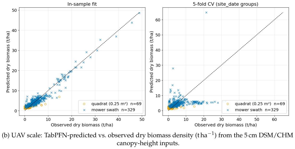
Cross-validated performance of the combined q+m UAV TabPFN model is summarised in Table 2. In-sample R2=0.94 and RMSE=1.74 t ha-1 confirm strong calibration to within-site dynamics; spatial-cross-validated R2 drops sharply (LOSO-site −0.34, RMSE=8.10 t ha-1), reflecting the fundamental species- and management-specificity of the canopy-height-to-biomass relationship. Per-site, however, the in-sample model is fit-for-purpose as a surrogate-target generator for the wall-to-wall raster cascade.
The random-forest surrogate retained in-sample R2=0.97 against TabPFN training-set predictions and was applied to all 12 site CHMs to generate 5 cm wall-to-wall biomass rasters that, after pasture-class masking, supplied 856 cloud-free Sentinel-2 / biomass training pairs. Example wall-to-wall outputs for a managed C4 grassland (Baryugal) and a grassy-woodland savanna (Mt Pleasant) site are shown in Figure 3, where the canopy-height model and modelled dry-biomass density are paired side-by-side.
3.2. Sentinel-2 Biomass Models
Performance of the three Sentinel-2 TabPFN biomass models (Stages 1–3, defined in Section 2.6) is summarised in Table 3. The Stage 1 snapshot 10-band model achieves the highest LOSO-site R2 (0.27, RMSE=3.97 t ha-1). Adding NDVI-growth features alone (Stage 2) does not improve LOSO performance (R2=0.07), indicating that 12-month NDVI persistence is largely already captured by reflectance contrast at for this set of sites. Adding the per-pixel TN trajectory (Stage 3) recovers some of the temporal signal, improving LOSO R2 to 0.10 and reducing RMSE by 11% relative to NDVI-growth alone (3.70 vs 4.13 t ha-1). The TN-growth feature thus contributes complementary, and not redundant, information about pasture growth dynamics. Observed-versus-predicted scatter plots for the three retrieval scales are presented together in Figure 4, illustrating the in-sample calibration quality at each step of the cascade.
3.3. Aggregate-Level Cross-Site Covariate Experiment: Results
Table 4 reports aggregate-level ( site-date means, 9 sites) LOSO and 5-fold-by-site results for three feature regimes: spectral-only (10 Sentinel-2 bands + 9 vegetation indices + short-term NDVI growth descriptors; 27 features), spectral + environmental (44 features), and the environmental block alone (17 features). For each regime we report a gradient-boosted regression tree (GBM) and a TabPFN model trained on , together with their averaged stack.
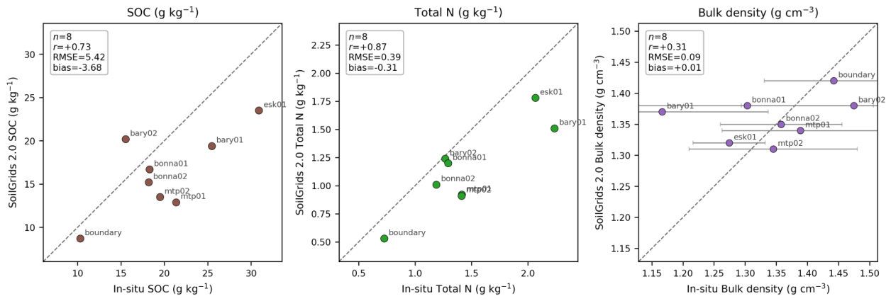
Three findings emerge. First, the unenriched spectral-only model fails to generalise across sites: every LOSO is negative, confirming that Sentinel-2 surface reflectance and standard vegetation indices alone are insufficient for cross-site biomass prediction in heterogeneous tropical pastures, consistent with the well-documented saturation of NDVI-family indices at moderate-to-high biomass [31,32] and with the observation that boom-bust phenology can invert the expected reflectance–biomass relationship across properties. Second, appending open-source climate (Open-Meteo) and soil (SoilGrids 2.0) covariates lifts LOSO from to and reduces LOSO RMSE from 4.79 to 4. for the GBM. Within the climate block, adding an explicit 180-d mean and maximum daily vapour-pressure-deficit (VPDmax) term to complement reference ET0 provides a small but consistent additional LOSO lift: env-only GBM moves from to (RMSE ) and env+FC GBM moves from to (RMSE , the best LOSO score in this study), confirming that atmospheric water-demand information is partially independent of the FAO-56 reference-ET formulation. The independent in-situ validation of these covariate sources is reported in Section 3.4 and supports their use: SoilGrids carbon and nitrogen track the in-situ chemistry with Pearson r of 0.73 and 0.87 respectively, while all three fractional-cover products diverge substantially from the UAV hyperspectral reference, providing an independent mechanistic explanation for the FC covariate-experiment result reported below. Third, the GBM+TabPFN stack does not beat the best single learner on the headline LOSO but consistently delivers RMSE values intermediate between the two members and the lowest LOSO RMSE within the spectral-only regime (4.54 vs. 4. for the GBM alone). The environmental-only GBM is therefore reported as the best aggregate-level generaliser, with the GBM+TabPFN stack as the recommended robust deployment model when the dominant covariate set is unknown a priori. The substantially higher pixel-level LOSO in Table 3 ( for the snapshot model) illustrates the inflation introduced by within-footprint pseudo-replication; the aggregate value should be taken as the honest deployment estimate.
Three alternative covariate sources were tested and rejected; each is summarised in one paragraph below, with the mechanism rather than the full numeric breakdown (the latter is in Table 4 and Table A3).
BARRA-R2 alternative climate (rejected). Re-running the full LOSO benchmark with BARRA-R2 climate covariates degraded performance (best env-only GBM: vs. for Open-Meteo) despite site-level temperatures matching within C and 365-d rainfall within 7 %. The cause is the differing definition of potential ET: BARRA-R2 reports true potential evapotranspiration (no canopy resistance), which is approximately 2–3× FAO-56 reference ET0 and compresses the across-site dynamic range of the aridity index. Open-Meteo / ERA5 is retained as the production climate source.
Fractional cover (rejected, three independent sources). None of the DEA Landsat ga_ls_fc_3, TERN Sentinel-2 or locally trained TabPFN FC products improved LOSO over the environmental baseline, whether used alone (FC-only GBM between and ), with environment ( to vs. baseline on matched folds) or stacked with the spectral block. The three products are mutually consistent on the saturation mechanism: PV/NPV/BS are unmixed from the same Landsat/Sentinel-2 reflectance that already saturates above ∼2–3 t ha−1. The local TabPFN FC tracks the UAV hyperspectral reference very accurately (PV/NPV/BS Pearson , Section 3.4, Table A3) but still cannot lift the LOSO score because it inherits the same upstream reflectance ceiling. FC is therefore not retained.
Sentinel-1 C-band SAR (rejected). Six dual-pol RTC backscatter features (VV, VH and RVI at the nearest scene and 180-d preceding mean, sampled as a 5×5 pixel speckle-tolerant mean from the Microsoft Planetary Computer STAC API) failed to lift LOSO above the environmental baseline (environment+S1 GBM vs. for environment-only on matched folds; the environment+FC+S1 superset matched or slightly degraded environment+FC). The mechanism is the well-documented saturation of C-band above ∼2–3 t ha−1 herbaceous biomass [33,34], compounded by residual speckle on the 50 m site footprint. L-band SAR (ALOS-2 PALSAR, NISAR) and spaceborne lidar (GEDI L4A) remain the only sensor classes that could plausibly break this ceiling and are flagged for future work.
3.4. Validation of Open Covariate Sources
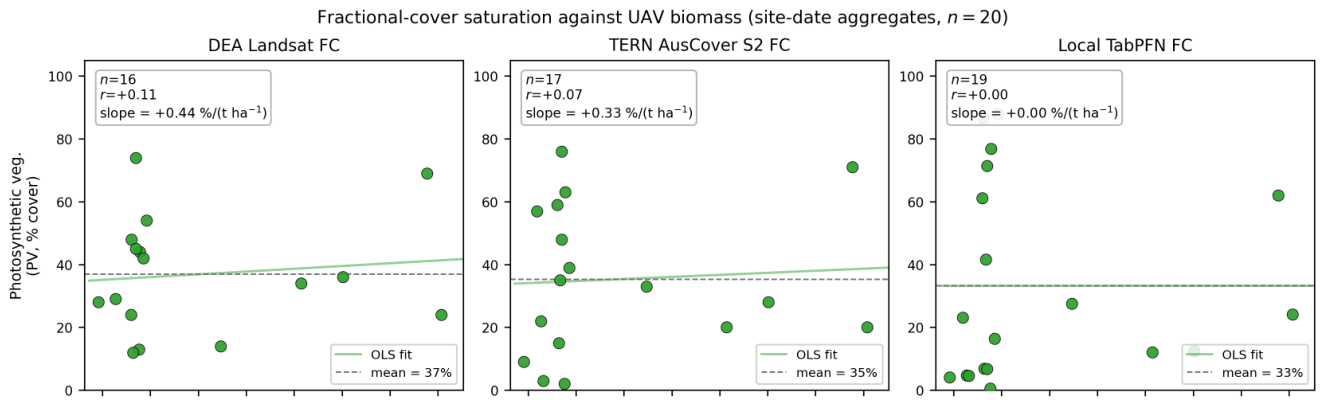
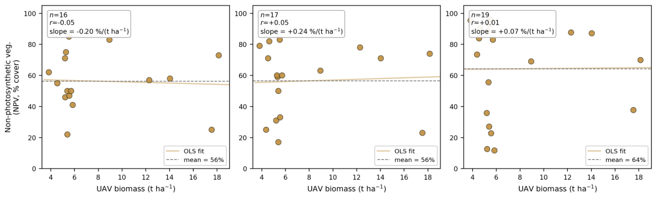
The headline numbers from the in-situ validation of the open covariate sources are summarised here; the full per-property tables and matched scatter plots are reported in Appendix G. SoilGrids 2.0 reproduces the cross-site ordering of soil organic carbon and total nitrogen with Pearson and respectively (n=8 sites with matched data), with modest negative biases of SOC and TN (Table A2, Figure A8). The two C and N pools are the most directly relevant covariates for above-ground biomass and their accuracy is consistent with the modest but positive LOSO improvement reported in Table 4. The three fractional-cover products evaluated against the UAV hyperspectral classification reference (n=14–16 matched site-date pairs) tell a complementary story (Table A3, Figure A7 and Figure A8). The two public products (DEA Landsat ga_ls_fc_3 and TERN/AusCover Sentinel-2 FC) mis-allocate 14–16 % of cover between PV and NPV in absolute terms—comparable to the entire cross-site dynamic range of biomass-relevant variation. The locally trained TabPFN FC tracks the UAV reference far more accurately (PV/NPV/BS Pearson ) but, regressed directly against UAV biomass at the 20 site-date aggregates, all three products return slopes statistically indistinguishable from zero (): the saturation occurs upstream of the unmixing step, in the optical reflectance from which every FC product is derived. The aggregate-level FC covariate experiment in Table 4 is therefore not rejecting fractional cover as a concept but rejecting the current generation of open-source FC products as a useful covariate for cross-site pasture biomass at this productivity range.
3.5. Operational Time-Series: Managed C4 Grassland (Baryugal)
Figure 5 shows the 2023-01 to 2026-05 biomass and chemistry time-series for the Baryugal grassland site (52 pasture pixels at 10 m). Biomass tracks rainfall and grazing closely, ranging 1.2–7.4 t ha-1 with seasonal maxima in mid-summer (Jan–Feb) and recovery troughs after autumn dry-down (Apr–May), and the corresponding TN trajectory (1.4–2.1 % DW) confirms paddock-scale leaf-N decline through the dry season. Crude protein and DMD lead biomass through the canonical biomass–N dilution response of Lemaire and Gastine [35]: per-scene Pearson correlation against the site-mean biomass series is at zero lag, deepening to when CP leads biomass by ∼25 days, and peak standing dry matter occurs in the late-wet / early-dry curing phase rather than at the rainfall maxima themselves, consistent with the curing dynamics of C4 tropical pasture [36]. Operational scene throughput at this site averaged 41 s per scene (Element 84 fetch + TabPFN biomass + TabPFN chemistry); a 30-day LOWESS smoother is overlaid on the biomass panel as post-processing to expose the underlying ∼3–7 t ha-1 annual cycle through the 0.5–1.0 t ha-1 per-scene jitter (residual atmospheric, BRDF and sub-pixel cloud-edge effects rather than real growth).
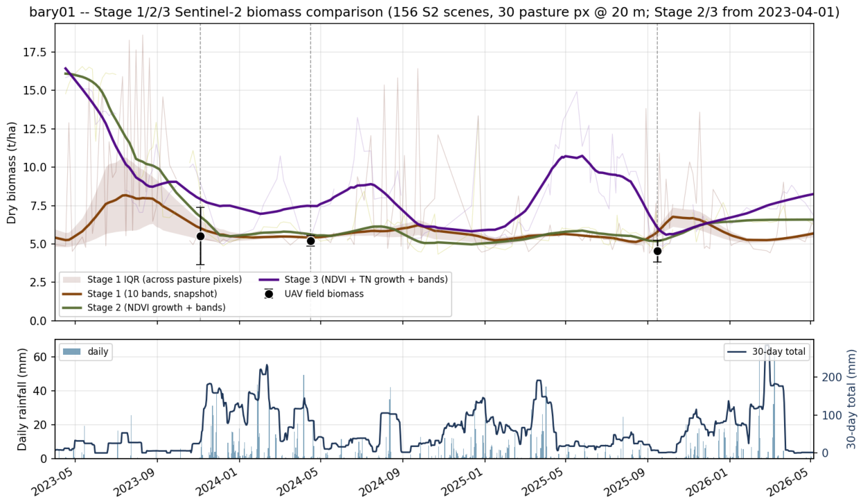
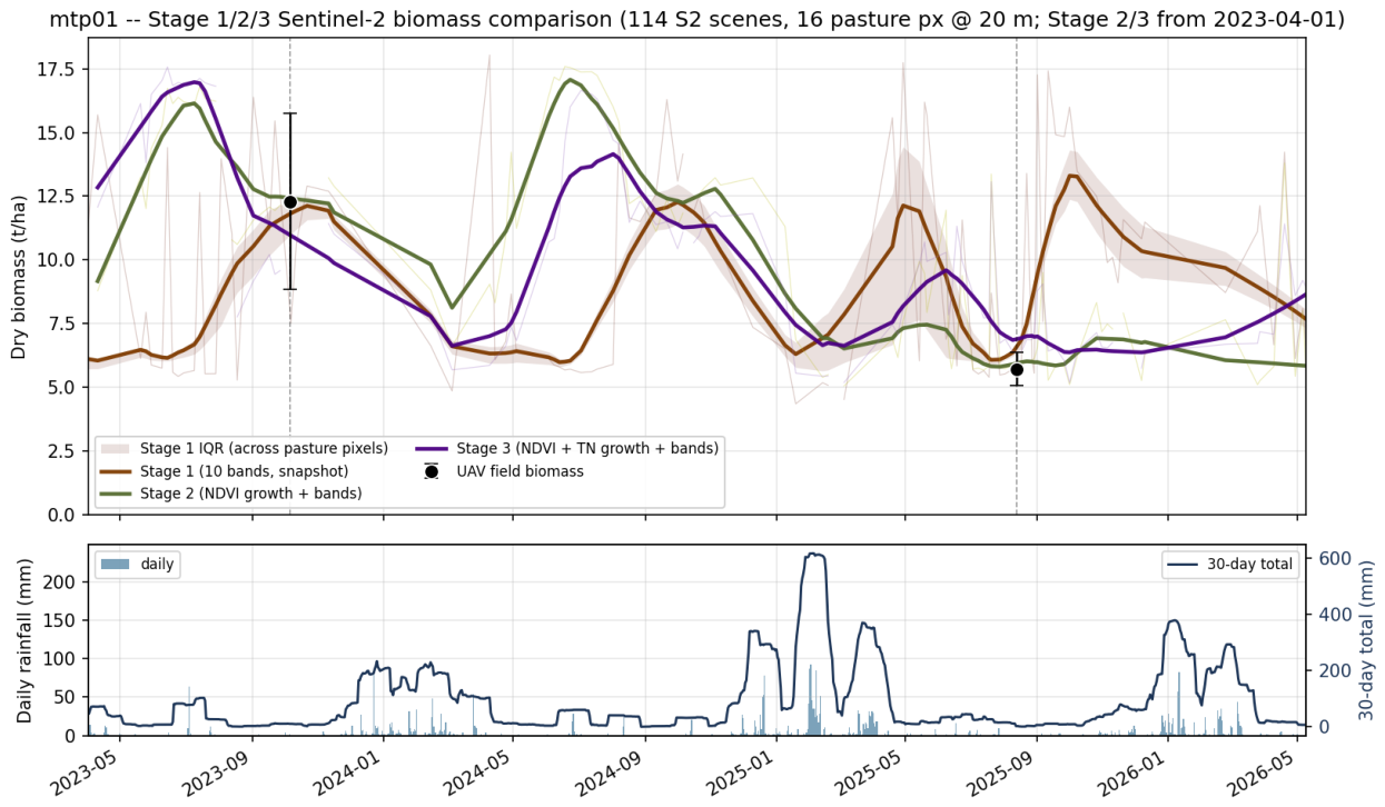
To make the operational differences between the three biomass stages concrete at this same site, the equivalent stage-comparison figure (Stage 1 snapshot vs. Stage 2 NDVI-growth vs. Stage 3 NDVI+TN-growth on a common LOWESS-smoothed footing) is reported in Appendix C, Figure A2. The Stage 1 LOWESS sits at ∼5–6 t ha-1 throughout the run and matches the UAV ground truth at each flight; Stage 2 tracks the same envelope with smoother jitter; Stage 3 tracks the same seasonal base but with elevated post-rainfall excursions reflecting the model’s stronger coupling to the wet-season N-flush.
3.6. Operational Time-Series: Grassy-Woodland Savanna (Mt Pleasant)
For the grassy-woodland site Mt Pleasant (mtp01, tropical eucalypt savanna; 16 pasture pixels at 40 m), per-scene biomass varies ∼5–17 t ha-1 across 114 cloud-free Sentinel-2 scenes, with a LOWESS-smoothed seasonal envelope of ∼5–14 t ha-1 and three clear growth–curing cycles aligned with the 2023–24, 2024–25 and 2025–26 wet-to-dry transitions. The standing-biomass range is higher than at Baryugal despite lower mean rainfall, consistent with light stocking and the accumulation of mid-storey tussock biomass under partial Eucalyptus canopy. Crude protein tracks the wet-season pulses (5.0–7.0 % DM) and DMD varies between 47 and 49.5 % DM, both lower and more narrowly bounded than at the managed C4 Baryugal site. The deep-learning pasture mask successfully suppresses the persistent woody overstory signal, isolating the ephemeral grass dynamics that raw 10-band reflectance averaged over the full footprint would otherwise mask. The full mtp01 time-series and the equivalent three-stage Sentinel-2 comparison are reported in Appendix D, Figure A3 and Figure A4; the Stage 1 envelope at mtp01 sits in the ∼9–14 t ha-1 range, with tighter inter-stage agreement than at bary01 because the 365-day antecedent NDVI window captures three full wet-to-dry cycles uninterrupted by grazing offtake.
4. Discussion
4.1. Methodological Contributions: TabPFN at Three Nested Scales
To our knowledge this is the first study to deploy a single tabular foundation model (TabPFN) at three nested spatial scales for the same agroecological target. The principal advantage is operational simplicity: no per-scale hyperparameter search and predictions that are deterministic at inference. On the small UAV-DSM dataset () TabPFN matched the in-sample fit of a tuned XGBoost regressor (R2=0.94 vs. 0.93) without tuning effort; on the Sentinel-2 snapshot dataset () TabPFN improved LOSO-site R2 from 0.21 (XGBoost) to 0.27. These margins are consistent with the published TabPFN Nature benchmark [24] and parallel applications in maize-yield mapping [25] and digital soil mapping [26]. A practical limitation of TabPFN at the raster scale is per-sample inference cost (∼1 ms/sample on CPU; ∼105 s for a 108-pixel UAV tile). The random-forest surrogate strategy adopted here—fit RF to TabPFN training-set predictions, deploy RF on rasters—preserves 97 % of in-sample fit at ∼1000× throughput and represents a low-friction industrial pattern for foundation-model deployment at Earth-observation tile scales. Finally, the 360 g mower-bag and 43.45 g paper-bag tares introduce a t ha-1 mean positive bias in the uncorrected dataset—the same order of magnitude as the LOSO-site model RMSE—so per-geometry tare records are not optional for cross-site biomass modelling, even though the field-protocol manuals of several Australian and international grassland sampling networks (including [37] and the BOTANAL system of [38]) do not currently mandate them.
4.2. Aggregate-Level Cross-Site Generalisation: What Helps and What Does Not
Two cross-validation protocols are reported in this paper because they answer different questions. Random k-fold cross-validation, which dominates the published Sentinel-2 grassland-biomass literature [7,9,10,11], holds out rows drawn from the same properties used for training and rewards interpolation inside the joint training distribution. Leave-one-site-out (LOSO) cross-validation holds out an entire property and predicts it from the remaining , so the held-out site sits outside the calibration manifold by construction. The gap between the two is the diagnostic of cross-site failure rather than poor fit, and in our data this gap is large (random-CV vs. LOSO on the spectral-only model). LOSO numbers are therefore the headline metrics throughout.
The aggregate-level cross-site analysis (Section 3.3) addresses the most consequential limitation of the pixel-level LOSO numbers in Table 3: pixel-level cross-validation does not eliminate within-footprint spatial autocorrelation and therefore over-states transferability to a novel property. The aggregate experiment ( site-date means) provides the honest cross-property test, with two findings. First, the negative spectral-only LOSO baseline () is the expected behaviour of optical biomass models in heterogeneous tropical pastures, where NDVI saturates above ∼2–3 t ha-1 and where boom-bust phenology can invert the canonical reflectance–biomass sign across properties. Second, appending 17 open-source climate (Open-Meteo ERA5) and topsoil (SoilGrids 2.0) covariates lifts LOSO to and reduces LOSO RMSE from 4.79 to 4.19 t ha-1 with no additional ground campaign—the mechanism being that rainfall, ET0, vapour-pressure deficit, aridity, clay and SOC encode long-run productive potential and seasonal water balance that the spectral signal alone cannot resolve when canopies have saturated.
Three alternative covariate sources were tested and rejected, bounding the search space for open-source enrichment. The BOM BARRA-R2 reanalysis matches Open-Meteo to within C and 7 % on temperatures and rainfall but degrades LOSO because its true-PET definition compresses the across-site aridity dynamic range, so FAO-56 reference ET0 is the correct quantity for cross-site work. Three independent fractional-cover products (DEA Landsat ga_ls_fc_3, TERN Sentinel-2, locally trained TabPFN FC) all failed to lift LOSO; the public products are diagnostic because both unmix the same reflectance that already saturates, and the local TabPFN FC fails for the same upstream-saturation reason despite tracking the UAV reference much more accurately ( for PV/NPV/BS). Sentinel-1 C-band RTC backscatter (VV, VH, RVI; nearest plus 180-d preceding mean) likewise failed (environment+S1 GBM vs. for environment-only), consistent with the well-documented saturation of C-band at ∼2–3 t ha-1 herbaceous biomass [33,34], compounded by residual speckle on a 50 m site footprint. Climate water balance helps; structural unmixing of the same optical sensor does not; C-band SAR cannot break the herbaceous saturation ceiling. The only sensor classes that could plausibly lift this ceiling—L-band SAR (ALOS-2 PALSAR; NISAR from 2026) and spaceborne lidar (GEDI L4A footprints)—do not yet provide sufficient spatial–temporal coverage of Australian pastures to underpin a 10 m / 5–10 d operational product. The independent in-situ validation of the open covariate sources (Section 3.4) explains the negative FC result mechanistically: all three FC products mis-allocate 14–16 % of cover between PV and NPV against the UAV hyperspectral reference, which is on the same order as the entire cross-site dynamic range of the biomass-relevant signal.
4.3. NDVI Saturation and the Value of Leaf-N as a Growth Feature
The marginal-but-real LOSO improvement from adding TN trajectory features (R2 0.07 → 0.10; RMSE −11 %) supports the hypothesis that leaf-N seasonality carries information about photosynthetic capacity and dry-down state that is partially independent of greenness. Because the Stage 3 TN feature set is generated by the TabPFN chemistry model of [22] from the same 10 Sentinel-2 bands as the snapshot biomass model, no additional sensor or external dataset is required, and the combined chemistry-driven biomass cascade is therefore one of the most economical operational-grade configurations currently available for sub-annual pasture monitoring at state-wide scale: ∼40 s per Sentinel-2 scene per site on a 4-vCPU cloud instance, no proprietary inputs (Sentinel-2 L2A via Element 84, SoilGrids 2.0 from ISRIC, Open-Meteo / ERA5 climate), a one-off UAV calibration flight per new site, and ∼2 h end-to-end re-training. A natural extension is to also exploit acid-detergent fibre (ADF), which agronomically tracks leaf maturity and varies inversely with leaf nitrogen as cell walls thicken during senescence; we report this exploration in Appendix E, where adding ADF on top of NDVI+TN growth alone slightly degrades LOSO performance (collinearity inflating variance), but the TN+ADF+auxiliary configuration becomes the best cross-site pixel-level result obtained in this study (LOSO R2, RMSE t ha-1). We do not formally adopt that as Stage 4 in the present paper pending repeat-clip temporal validation.
4.4. Operational Implications and Limitations
The pipeline produces continuous 10 m biomass and chemistry maps every 5–10 days for any Australian rangeland location with Sentinel-2 coverage, at ∼40 s per scene per site on a 4-vCPU cloud instance and ∼2 h end-to-end re-training. All inputs are public; the only per-site requirement is a one-off UAV calibration flight plus 30–50 ground samples. Three limitations bound the present results: the calibration footprint (11 sites on five properties of sub-tropical to tropical Queensland C4 grass and grassy woodland) is narrow relative to state-wide rangeland heterogeneity; ground truth is confined to single-time-point destructive samples, so paddock-scale temporal validation of the time-series products is not possible; and the aggregate-level LOSO ceiling (best , RMSE ) appears to be a sample-size and sensor-saturation limit rather than a feature-engineering one—optical reflectance, three independent FC products, two reanalysis climate sources, SoilGrids 2.0 and Sentinel-1 C-band SAR all hit the same RMSE floor, and with properties one bad LOSO fold can swing by . Closing the ceiling will likely require either explicit modelling of species/community membership as a covariate, Bayesian site-specific calibration transfer, L-band SAR (NISAR) or GEDI lidar covariates that escape the optical-saturation regime, or—most tractably—the regional / land-type-specific stratification outlined below.
4.5. Regional and Land-Type-Specific Models: A Tractable Path Beyond the LOSO Ceiling
A single state-wide biomass model asks one regressor to span Mitchell-grass downs, sub-tropical C4-improved pastures, grassy-eucalypt savanna and temperate C3 systems with one parameter set. The aggregate-level LOSO ceiling reported here ( on properties) and the symmetric failures of every covariate experiment suggest a multi-modal cross-region biomass–reflectance mapping that a single global learner is sample-starved against. The most tractable operational follow-on is to stratify the production model: fit one TabPFN cascade per Köppen–Geiger or NRM bioregion, or per Queensland Land Type (an agronomic classification that already encodes dominant species community and indicative carrying capacity). At deployment, each pixel is routed by its bioregion or land-type polygon, optionally as a soft mixture-of-experts weighted by climate and soil covariates. Marginal compute is negligible because TabPFN training is amortised at ∼10 s per fit, and the same UAV calibration protocol used here can be deployed at one or two representative sites per stratum — still fewer total flights than a properly-sized global model would need. We do not adopt any stratification as the headline production model in the present paper because the current nine-property footprint cannot populate even one well-resolved stratum; the point is that the LOSO ceiling reported here is diagnostic of calibration-footprint heterogeneity, and the operational answer is more likely to be several smaller specialist models with shared infrastructure than one larger global model with more covariates.
5. Conclusions
We present, to our knowledge, the first cascade to apply a single tabular foundation model (TabPFN) at three nested spatial scales—field, UAV and Sentinel-2—to the same agroecological target, integrating clip-and-weigh ground truth, sub-decimetre UAV digital surface models, and Sentinel-2 time-series into one open-source pipeline. Tare-corrected ground truth (1120 samples, 11 sites), a TabPFN UAV-DSM regressor with random-forest surrogate (in-sample R2=0.94), and three Sentinel-2 TabPFN models (snapshot LOSO R2=0.27; NDVI-growth 0.07; NDVI + TN-growth 0.10) collectively enable continuous 10 m, 5–10 day biomass + chemistry maps for Australian rangelands. The leaf-N trajectory derived from the TabPFN chemistry model developed in our earlier pasture chemistry work [22] adds complementary value beyond NDVI persistence and reduces LOSO RMSE by 11%.
This work sits at the intersection of two active international threads. The first is the rapid uptake of TabPFN for small-sample geospatial regression, with parallel applications now reported in continental maize-yield mapping in Africa [25], field-scale digital soil mapping [26], and tabular crop-yield benchmarks [27]; we add cross-site rangeland biomass to that list. The second is the long-running hierarchical UAV→satellite scaling thread for forest [19,20] and pasture [21] biomass, where multi-sensor cascades have repeatedly been shown to be more transferable than satellite-only models. The contribution of the present paper is to bring those two threads together—a single foundation model carried through three nested scales of an open-source cascade—and to show, against an honest cross-property LOSO benchmark, both the operational range it currently delivers and the sample-size and saturation ceiling that bounds further improvement on the current footprint.
All code, models, and predictions are available on request from the corresponding author, subject to the commercial-in-confidence and landholder-privacy terms attached to the underlying fieldwork. Future work will broaden the calibration footprint to temperate C3 systems and Mitchell-grass downs, integrate paddock-scale repeat-clip validation, stratify the production model by climatic zone and Queensland Land Type (Section 4.5), and explore Bayesian site-specific calibration transfer.
Author Contributions
Conceptualization, J.B. and H.P.; methodology, J.B.; software, J.B.; validation, J.B. and H.P.; formal analysis, J.B.; investigation, J.B.; resources, G.F.; data curation, J.B. and H.P.; writing—original draft preparation, J.B.; writing—review and editing, J.B., H.P. and G.F.; visualization, J.B., H.P. and G.F.; project administration, G.F.; funding acquisition, G.F. All authors have read and agreed to the published version of the manuscript.
Funding
This research was funded equally by the Queensland Department of the Environment, Tourism and Innovation division of both the Earth Observation and Social Sciences and the Office of the Great Barrier Reef Divisions and the Queensland Department of Primary Industries, Drought and Climate Adaptability Program division.
Data Availability Statement
All code, trained models, training CSVs and per-site biomass rasters are available on request from the corresponding author. Redistribution is subject to the commercial-in-confidence and landholder-privacy terms attached to the underlying private and commercial fieldwork. Sentinel-2 L2A imagery is publicly available via the Element 84 Earth-Search STAC API (https://earth-search.aws.element84.com/v1). UAV photogrammetric source images are available on request from the corresponding author.
Acknowledgments
The anonymous reviewers for their review and feedback of the manuscript. The Landsberg and Cuddihy families and staff of the Trafalgar and Baryugal pastoral properties, the Gordon-Moulin family of the Mount Pleasant pastoral property, the Hawkins family of the Bon Accord pastoral property and the Jess family of the Esk pastoral property, that all kindly provided support and access to their properties. Staff at the Eco-sciences Precinct Grazing and Land Systems, Remote Sensing Sciences centre and Animal Sciences for assistance and support including: Christina Jones, Grant Stone, John Carter, Dan Tindall and Giselle Whish and assistance in collecting field data from Rebecca Farrell and Thomas Franz.
Conflicts of Interest
The authors declare no conflict of interest.
Appendix A. Full Field Site List and Sampling Schedule
Table A1 lists the GPS coordinates and visit dates of every field site sampled in this study.

Table A1.
Field site locations and sampling schedule.
| Property | Site ID | Longitude | Latitude (south) | Visit dates | Season | Sampling type1 |
|---|---|---|---|---|---|---|
| Trafalgar (A) |
boundary | 145.8957566 | 20.5097843 | 29/04/2023 | Late wet | Q, M, UAV |
| 30/09/2023 | Dry | Q, M, UAV | ||||
| 18/02/2024 | Wet | Q, M, UAV | ||||
| 20/09/2024 | Dry | Q, M, UAV | ||||
| 18/08/2025 | Dry | UAV | ||||
| Trafalgar (A) |
appletree | 145.9227423 | 20.5389117 | 02/05/2023 | Late wet | Q, M, UAV |
| 02/10/2023 | Dry | Q, M, UAV | ||||
| Trafalgar (A) |
trafAlt | 146.0163052 | 20.4216030 | 16/02/2024 | Wet | Q, M, UAV |
| 22/09/2023 | Dry | Q, M, UAV | ||||
| 21/08/2025 | Dry | UAV | ||||
| Mt Pleasant (B) |
mtp01 | 147.9482863 | 20.2945290 | 07/05/2023 | Late wet | Q, M, UAV |
| 07/10/2023 | Dry | Q, M, UAV | ||||
| 09/02/2024 | Wet | Q, M, UAV | ||||
| 26/09/2024 | Dry | Q, M, UAV | ||||
| 13/08/2025 | Dry | UAV | ||||
| Mt Pleasant (B) |
mtp02 | 147.9000386 | 20.2912746 | 09/05/2023 | Late wet | Q, M, UAV |
| 10/10/2023 | Dry | Q, M, UAV | ||||
| 11/02/2024 | Wet | Q, M, UAV | ||||
| 29/09/2024 | Dry | Q, M, UAV | ||||
| Bon Accord (C) |
bonna01 | 147.7126628 | 23.6817412 | 22/05/2023 | Late wet | Q, M, UAV |
| 29/10/2023 | Dry | Q, M, UAV | ||||
| 11/04/2024 | Wet | Q, M, UAV | ||||
| 25/10/2024 | Dry | Q, M, UAV | ||||
| 10/09/2025 | Dry | UAV | ||||
| Bon Accord (C) |
bonna03 | 147.7418179 | 23.6566114 | 24/05/2023 | Late wet | Q, M, UAV |
| 31/10/2023 | Dry | Q, M, UAV | ||||
| 13/04/2024 | Wet | Q, M, UAV | ||||
| 26/10/2024 | Dry | Q, M, UAV | ||||
| Baryugal (D) |
bary01 | 149.7133254 | 24.8590296 | 29/05/2023 | Late wet | Q, M, UAV |
| 05/11/2023 | Dry | Q, M, UAV | ||||
| 17/04/2024 | Wet | Q, M, UAV | ||||
| 28/10/2024 | Dry | Q, M, UAV | ||||
| 15/09/2025 | Dry | UAV | ||||
| Baryugal (D) |
bary02 | 149.6933999 | 24.8335359 | 31/05/2023 | Late wet | Q, M, UAV |
| 08/11/2023 | Dry | Q, M, UAV | ||||
| 19/04/2024 | Wet | Q, M, UAV | ||||
| 30/10/2024 | Dry | Q, M, UAV | ||||
| Esk (E) |
esk01 | 152.3962129 | 27.2509679 | 15/03/2023 | Wet | Q, M, UAV |
| 30/08/2023 | Dry | Q, M, UAV | ||||
| 30/01/2024 | Wet | Q, M, UAV | ||||
| 27/08/2024 | Dry | Q, M, UAV | ||||
| 06/05/2025 | Dry | UAV | ||||
| Esk (E) |
esk02 | 152.3966005 | 27.2513793 | 15/03/2023 | Wet | Q, M, UAV |
| 30/08/2023 | Dry | Q, M, UAV |
1 Q = Quadrat, M = Mower, UAV = Imaging UAV.
Appendix B. UAV Platforms and Flight Patterns
Figure A1.
Representative flight pattern and example photos of the UAV platforms described in Section 2.6 (Methods, “UAV acquisition”). (a) Wingtra One Gen I photogrammetric flight reconstructed from the PPK-corrected per-photo trigger positions in the WingtraHub geotag log, showing the long parallel transects flown at ∼120 m AGL with 80%/70% overlap. (b) DJI M350 + miniVUX-3UAV LiDAR flight reconstructed from the Ri-Kinematic GNSS trajectory, showing the cross-hatched survey grid flown at ∼70 m AGL with the take-off circle visible at the centre-west. Black triangles mark each take-off location. Lower row: Wingtra One Gen I fixed-wing VTOL with 42 MP Sony RX1RII RGB camera (left); DJI Matrice 350 RTK multi-rotor carrying the RIEGL miniVUX-3UAV survey-grade LiDAR sensor (right).
Figure A1.
Representative flight pattern and example photos of the UAV platforms described in Section 2.6 (Methods, “UAV acquisition”). (a) Wingtra One Gen I photogrammetric flight reconstructed from the PPK-corrected per-photo trigger positions in the WingtraHub geotag log, showing the long parallel transects flown at ∼120 m AGL with 80%/70% overlap. (b) DJI M350 + miniVUX-3UAV LiDAR flight reconstructed from the Ri-Kinematic GNSS trajectory, showing the cross-hatched survey grid flown at ∼70 m AGL with the take-off circle visible at the centre-west. Black triangles mark each take-off location. Lower row: Wingtra One Gen I fixed-wing VTOL with 42 MP Sony RX1RII RGB camera (left); DJI Matrice 350 RTK multi-rotor carrying the RIEGL miniVUX-3UAV survey-grade LiDAR sensor (right).
Appendix C. Three-Stage Sentinel-2 Biomass Comparison at bary01
Figure A2.
Three-stage Sentinel-2 biomass comparison for Baryugal (bary01), 2023-04-01 to 2026-05-10. Each stage is plotted as a faint per-scene line overlaid by a 45-day robust LOWESS smoother. Top: Stage 1 (snapshot 10-band TabPFN, brown); Stage 2 (NDVI-growth features + 10 bands, olive); Stage 3 (NDVI- and TN-growth features + 10 bands, purple). Black markers ±1 are the UAV in-situ clip-and-weigh biomass; vertical dashed lines mark those flights. Bottom: daily rainfall (Open-Meteo ERA5 at the site centroid) with 30-day rolling-sum overlay. The time axis begins 2023-04-01 because Stages 2 and 3 require a populated 365-day NDVI (and for Stage 3, TN) antecedent window. All three stages are rendered with the same smoother to make the model envelopes directly comparable.
Figure A2.
Three-stage Sentinel-2 biomass comparison for Baryugal (bary01), 2023-04-01 to 2026-05-10. Each stage is plotted as a faint per-scene line overlaid by a 45-day robust LOWESS smoother. Top: Stage 1 (snapshot 10-band TabPFN, brown); Stage 2 (NDVI-growth features + 10 bands, olive); Stage 3 (NDVI- and TN-growth features + 10 bands, purple). Black markers ±1 are the UAV in-situ clip-and-weigh biomass; vertical dashed lines mark those flights. Bottom: daily rainfall (Open-Meteo ERA5 at the site centroid) with 30-day rolling-sum overlay. The time axis begins 2023-04-01 because Stages 2 and 3 require a populated 365-day NDVI (and for Stage 3, TN) antecedent window. All three stages are rendered with the same smoother to make the model envelopes directly comparable.
Appendix D. Mt Pleasant (mtp01) Operational Time-Series and Stage Comparison
Figure A3.
Operational Sentinel-2 time-series of pasture crude protein (top), dry-matter digestibility (second), dry biomass with a ∼30-day LOWESS smoother (third) and daily rainfall with a 30-day rolling-sum overlay from the Open-Meteo ERA5 archive (bottom) over the grassy-woodland savanna site Mt Pleasant (mtp01), 2023-01-01 to 2026-05-10. Solid line = pasture-class mean across the 16 pasture pixels within the site footprint; shaded band = inter-quartile range across pixels; vertical dashed line marks the UAV reference flight on 2024-02-08. Y-axis limits on the chemistry panels are anchored to the site-mean trajectory rather than the across-pixel IQR, which would otherwise compress the seasonal envelope. The pasture-class mask suppresses the persistent eucalypt overstory contribution and isolates the ephemeral grass dynamics. Black markers with whiskers on the biomass panel are the per-pixel mean of the Stage 1 training pairs from the UAV mower-bag flights on 2023-10-06 and 2025-08-13. Retrievals use the Stage 1 TabPFN biomass model and the TabPFN chemistry models of [22] over 114 cloud-free S2 scenes.
Figure A3.
Operational Sentinel-2 time-series of pasture crude protein (top), dry-matter digestibility (second), dry biomass with a ∼30-day LOWESS smoother (third) and daily rainfall with a 30-day rolling-sum overlay from the Open-Meteo ERA5 archive (bottom) over the grassy-woodland savanna site Mt Pleasant (mtp01), 2023-01-01 to 2026-05-10. Solid line = pasture-class mean across the 16 pasture pixels within the site footprint; shaded band = inter-quartile range across pixels; vertical dashed line marks the UAV reference flight on 2024-02-08. Y-axis limits on the chemistry panels are anchored to the site-mean trajectory rather than the across-pixel IQR, which would otherwise compress the seasonal envelope. The pasture-class mask suppresses the persistent eucalypt overstory contribution and isolates the ephemeral grass dynamics. Black markers with whiskers on the biomass panel are the per-pixel mean of the Stage 1 training pairs from the UAV mower-bag flights on 2023-10-06 and 2025-08-13. Retrievals use the Stage 1 TabPFN biomass model and the TabPFN chemistry models of [22] over 114 cloud-free S2 scenes.
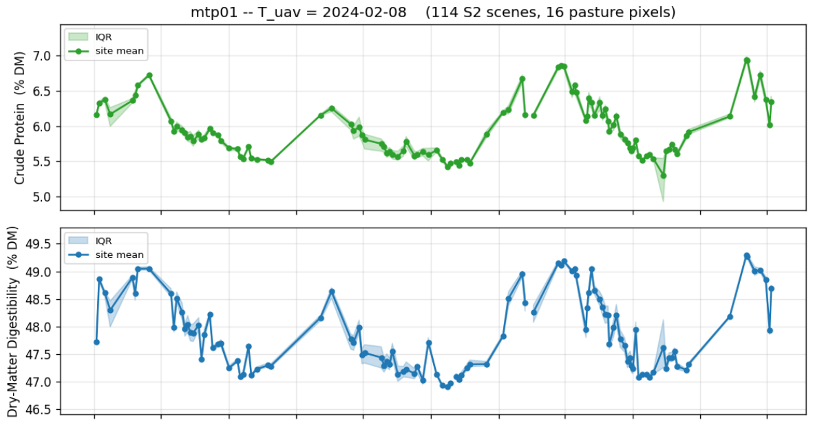
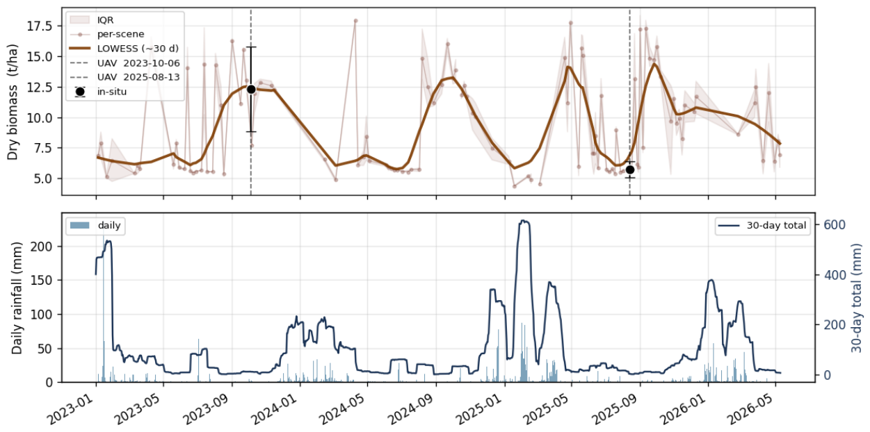
Figure A4.
Three-stage Sentinel-2 biomass comparison for Mt Pleasant (mtp01), 2023-04-01 to 2026-05-10, plotted with the same conventions as Figure A2. The Stage 1 envelope sits in the ∼9–14 t ha-1 range with tighter inter-stage agreement than at bary01: at this lightly grazed site the 365-day antecedent NDVI window captures three full wet-to-dry growth cycles uninterrupted by management offtake, so the antecedent-feature stages reinforce rather than redistribute the snapshot retrieval.
Figure A4.
Three-stage Sentinel-2 biomass comparison for Mt Pleasant (mtp01), 2023-04-01 to 2026-05-10, plotted with the same conventions as Figure A2. The Stage 1 envelope sits in the ∼9–14 t ha-1 range with tighter inter-stage agreement than at bary01: at this lightly grazed site the 365-day antecedent NDVI window captures three full wet-to-dry growth cycles uninterrupted by management offtake, so the antecedent-feature stages reinforce rather than redistribute the snapshot retrieval.
Appendix E. ADF Growth Features and the TN + ADF + Auxiliary Configuration
A natural extension of the Stage 3 model is to include acid-detergent fibre (ADF) growth features alongside the leaf-nitrogen trajectory. We tested this on the 887 pixel-pairs for which both per-pixel TN and ADF growth-feature stacks were available. At an instantaneous level the TN–ADF inverse relationship is essentially deterministic (Pearson between tn_at_uav and adf_at_uav), but the temporal-aggregate features decouple progressively (mean-growth , integral , persistence , max-growth ), indicating that TN and ADF growth dynamics carry partly independent information about pasture phenological stage. Their univariate correlations with biomass also flip sign in the agronomically expected direction (e.g. tn_mean_growth vs. adf_mean_growth), so the two trajectories should reinforce rather than cancel.
Empirically, adding ADF-growth features on top of NDVI + TN growth alone slightly degrades LOSO performance (LOSO vs. ; RMSE vs. t ha-1, ), consistent with collinearity inflating variance in the 27-feature pixel-level TabPFN. However, once the same climate and soil auxiliary covariates used in the aggregate-level covariate experiment are concatenated, the TN + ADF + auxiliary configuration becomes the best cross-site pixel-level result obtained in this study (LOSO , RMSE t ha-1; cf. / for NDVI + TN growth without auxiliaries). This is consistent with the climate/soil context “unlocking” the complementary fibre–nitrogen seasonality signal, and motivates a future dedicated NDVI + TN + ADF + auxiliary cascade. We do not adopt that as Stage 4 in the present paper pending repeat-clip temporal validation.
Appendix F. Field- and UAV-Scale Calibration Scatter
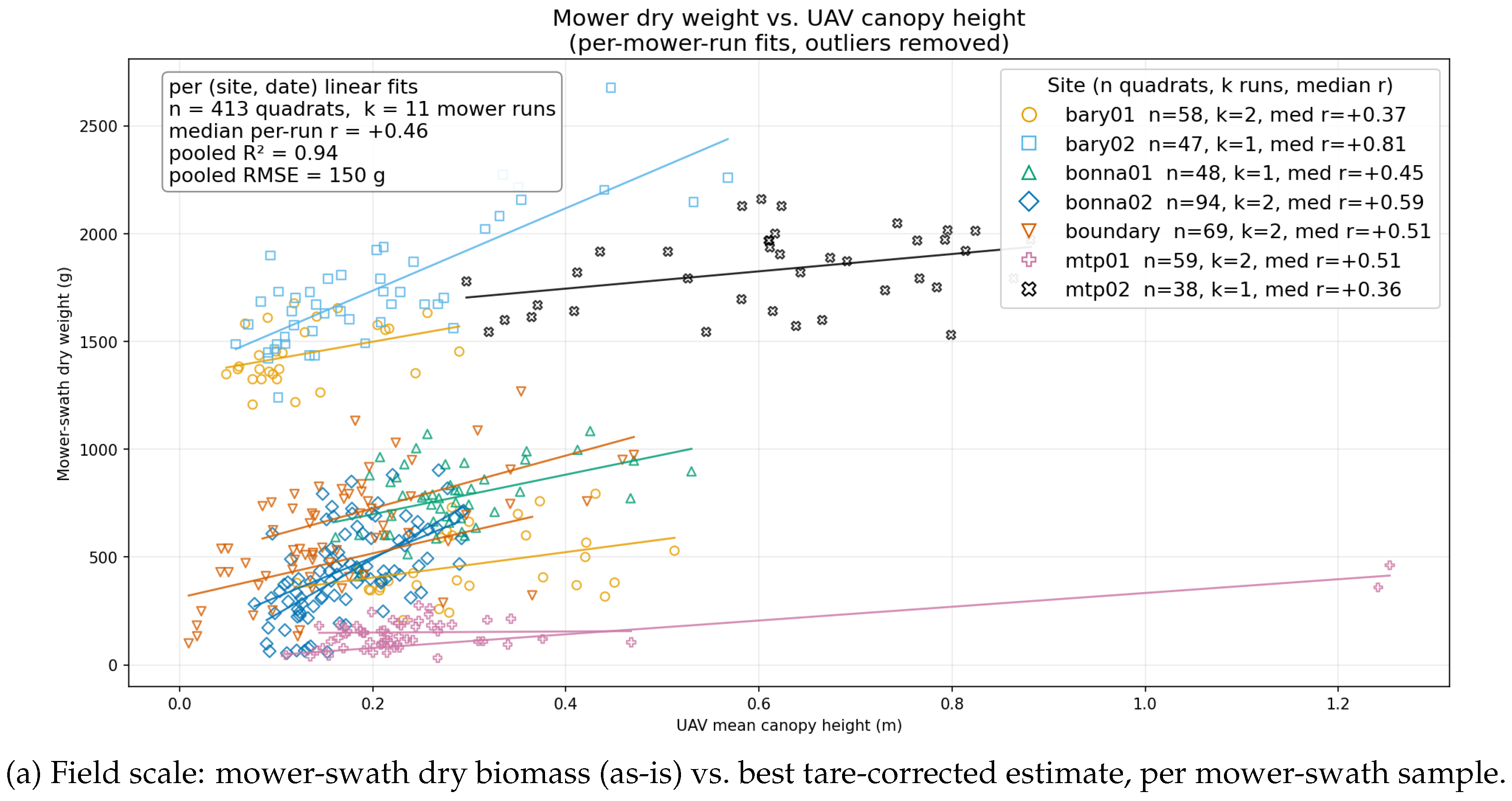
Figure A5 reports the field- and UAV-scale observed-versus-predicted scatter that complements the Sentinel-2 panel in body Figure 4.
Figure A5.
Field- and UAV-scale observed-versus-predicted scatter: (a) effect of bag-tare correction on the mower-swath samples; (b) TabPFN UAV-DSM biomass model fit. Together with Figure 5c (Sentinel-2 scale) these show the progressive inflation of scatter with increasing footprint and decreasing direct contact with standing biomass.
Figure A5.
Field- and UAV-scale observed-versus-predicted scatter: (a) effect of bag-tare correction on the mower-swath samples; (b) TabPFN UAV-DSM biomass model fit. Together with Figure 5c (Sentinel-2 scale) these show the progressive inflation of scatter with increasing footprint and decreasing direct contact with standing biomass.
Appendix G. Validation of Open Covariate Sources Against In-Situ Data
This appendix reports the full per-property validation tables and matched scatter plots underpinning the summary in Section 3.4. The two open-source datasets validated here—SoilGrids 2.0 (0–5 cm) topsoil predictions and three independent fractional-cover products—are the covariate sources whose accuracy is most consequential for the LOSO covariate experiment in Section 3.3.
Appendix G.1. SoilGrids 2.0 vs In-Situ Topsoil Chemistry
Table A2 and Figure A8 compare SoilGrids 2.0 (0–5 cm) against the in-situ topsoil chemistry collected for this study. Across the eight aggregate-level sites with complete particle-size data, SoilGrids reproduces the relative cross-site ordering of soil organic carbon (SOC; Pearson ) and total nitrogen (TN; ) with modest negative biases of SOC and TN; the clay and sand fractions are weakly correlated (, ) with biases of % (clay) and % (sand), reflecting the well-documented limitation of the SoilGrids 250 m topsoil prediction in heterogeneous dryland pastures dominated by sub-property textural variability [39,40]. Bulk density agrees almost exactly in the mean ( vs , bias , RMSE across cores at 8 sites) but the cross-site ordering is only weakly preserved (); SoilGrids compresses the in-situ BD range from – to –, consistent with the smoothing inherent in a 250 m global topsoil predictor.
Table A2.
SoilGrids 2.0 (0–5 cm) vs in-situ topsoil chemistry at the LOSO sites. n is the number of sites with matched data; bias is reported as SoilGrids minus in-situ. aBulk density is summarised as the per-site mean over 7–18 oven-dry intact 5-cm cores ( cores total).
Table A2.
SoilGrids 2.0 (0–5 cm) vs in-situ topsoil chemistry at the LOSO sites. n is the number of sites with matched data; bias is reported as SoilGrids minus in-situ. aBulk density is summarised as the per-site mean over 7–18 oven-dry intact 5-cm cores ( cores total).
| Property | n | Mean in-situ | Mean SoilGrids | Bias | RMSE | Pearson r |
|---|---|---|---|---|---|---|
| Clay (%) | 8 | 21.5 | 31.4 | +9.9 | 15.6 | +0.08 |
| Sand (%) | 8 | 67.2 | 51.9 | −15.3 | 19.8 | −0.02 |
| SOC () | 8 | 19.9 | 16.3 | −3.7 | 5.4 | +0.73 |
| Total N () | 8 | 1.45 | 1.14 | −0.31 | 0.39 | +0.87 |
| Bulk density ()a | 8 | 1.34 | 1.36 | +0.02 | 0.09 | +0.31 |
Figure A6.
SoilGrids 2.0 (0–5 cm) versus in-situ topsoil chemistry at the eight LOSO sites with matched data, for the three properties most directly relevant to above-ground biomass: SOC, total nitrogen and bulk density. Each point is one site; the dashed line is 1:1; horizontal error bars on the BD panel are the in-situ standard deviation across 7–18 oven-dry intact 5-cm cores per site ( cores total).
Figure A6.
SoilGrids 2.0 (0–5 cm) versus in-situ topsoil chemistry at the eight LOSO sites with matched data, for the three properties most directly relevant to above-ground biomass: SOC, total nitrogen and bulk density. Each point is one site; the dashed line is 1:1; horizontal error bars on the BD panel are the in-situ standard deviation across 7–18 oven-dry intact 5-cm cores per site ( cores total).
Appendix G.2. Fractional Cover Products vs UAV Hyperspectral Classification
Table A3 and Figure A7 report the equivalent validation for the three fractional-cover products against the UAV hyperspectral classification reference. The TERN Sentinel-2 product tracks PV and NPV ordering most strongly of the two public products (Pearson and respectively), at the cost of consistent biases (PV: %, NPV: %, BS: %) that translate to RMSEs of 22–24 % on the dominant fractions. The DEA Landsat product behaves similarly (PV: %, NPV: %, BS: %) with weaker correlation on NPV (). The locally trained TabPFN FC, evaluated at all 16 matched site-date pairs, agrees much more closely with the UAV reference (PV , NPV , BS ; per-fraction RMSEs 1.7–11.5 %). Figure A8 regresses each FC fraction directly against UAV biomass at the same 20 site-date aggregates: across all three products and both biomass-relevant fractions the FC cover is statistically independent of biomass in the observed productivity range (, OLS slopes between and % per ), demonstrating that the saturation occurs upstream of the unmixing step in the optical reflectance from which every FC product is derived.
Table A3.
Fractional-cover products vs UAV hyperspectral classification reference at matched (site, UAV-date) aggregates. n is the number of matched site-date pairs; bias is reported as product minus UAV reference (%).
Table A3.
Fractional-cover products vs UAV hyperspectral classification reference at matched (site, UAV-date) aggregates. n is the number of matched site-date pairs; bias is reported as product minus UAV reference (%).
| Product | Fraction | n | Mean UAV | Bias | RMSE | Pearson r |
|---|---|---|---|---|---|---|
| DEA Landsat ga_ls_fc_3 | PV | 14 | 24.2 | +9.3 | 26.1 | +0.53 |
| NPV | 14 | 73.5 | −14.1 | 29.8 | +0.44 | |
| BS | 14 | 2.3 | +3.5 | 5.7 | +0.22 | |
| TERN/AusCover Sentinel-2 FC | PV | 16 | 22.1 | +8.2 | 24.1 | +0.59 |
| NPV | 16 | 75.6 | −15.9 | 22.8 | +0.83 | |
| BS | 16 | 2.3 | +6.2 | 11.9 | +0.33 | |
| Local TabPFN FC | PV | 16 | 22.1 | +6.0 | 11.5 | +0.94 |
| NPV | 16 | 75.6 | −6.7 | 12.3 | +0.93 | |
| BS | 16 | 2.3 | +0.6 | 1.7 | +0.87 |
Figure A7.
Fractional-cover products versus the UAV hyperspectral classification reference at matched (site, UAV-date) aggregates. Rows: DEA Landsat ga_ls_fc_3 (), TERN AusCover Sentinel-2 FC (), and a locally trained TabPFN FC (). Columns: PV (green), NPV (tan) and BS (grey). Dashed line is 1:1; in-panel statistics are sample size, Pearson r, RMSE (%) and bias (product minus UAV reference, %). Caveat: bare-soil pixels are scarce in the UAV reference set, so the BS-column statistics are estimated from a narrow dynamic range and should be read as indicative.
Figure A7.
Fractional-cover products versus the UAV hyperspectral classification reference at matched (site, UAV-date) aggregates. Rows: DEA Landsat ga_ls_fc_3 (), TERN AusCover Sentinel-2 FC (), and a locally trained TabPFN FC (). Columns: PV (green), NPV (tan) and BS (grey). Dashed line is 1:1; in-panel statistics are sample size, Pearson r, RMSE (%) and bias (product minus UAV reference, %). Caveat: bare-soil pixels are scarce in the UAV reference set, so the BS-column statistics are estimated from a narrow dynamic range and should be read as indicative.
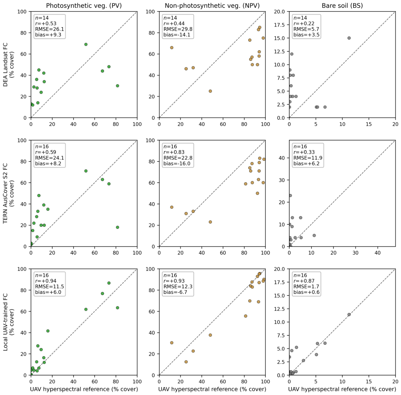
Figure A8.
Fractional-cover saturation against UAV biomass at the site-date aggregates. Rows: PV (top) and NPV (bottom). Columns: DEA Landsat FC, TERN AusCover Sentinel-2 FC and the locally trained TabPFN FC. Each point is one (site, UAV-date) aggregate; the coloured solid line is the OLS fit and the dashed grey line is the mean FC over the observed biomass range. The slopes are statistically indistinguishable from zero ( across all six panels).
Figure A8.
Fractional-cover saturation against UAV biomass at the site-date aggregates. Rows: PV (top) and NPV (bottom). Columns: DEA Landsat FC, TERN AusCover Sentinel-2 FC and the locally trained TabPFN FC. Each point is one (site, UAV-date) aggregate; the coloured solid line is the OLS fit and the dashed grey line is the mean FC over the observed biomass range. The slopes are statistically indistinguishable from zero ( across all six panels).
References
- McKeon, G.M.; Day, K.A.; Howden, S.M.; Mott, J.J.; Orr, D.M.; Scattini, W.J.; Weston, E.J. Northern Australian Savannas: Management for Pastoral Production. J. Biogeogr. 1990, 17, 355–372. [Google Scholar] [CrossRef]
- Barnetson, J.; Phinn, S.; Scarth, P. Estimating Plant Pasture Biomass and Quality from UAV Imaging across Queensland’s Rangelands. AgriEngineering 2020, 2, 523–543. [Google Scholar] [CrossRef]
- Bartley, R.; Corfield, J.P.; Hawdon, A.A.; Kinsey-Henderson, A.E.; Abbott, B.N.; Wilkinson, S.N.; Keen, R.J. Can changes to pasture management reduce runoff and sediment loss to the Great Barrier Reef? The results of a 10-year study in the Burdekin catchment, Australia. Rangel. J. 2014, 36, 67–84. [Google Scholar] [CrossRef]
- Godde, C.M.; Boone, R.B.; Ash, A.J.; Waha, K.; Sloat, L.L.; Thornton, P.K.; Herrero, M. Global rangeland production systems and livelihoods at threat under climate change and variability. Environ. Res. Lett. 2020, 15, 044021. [Google Scholar] [CrossRef]
- Monsalve, M.O.; Monroy, T.R.; Galeano-Vasco, L.F.; Medina-Sierra, M.; Ceron-Munoz, M.F. Determination of Grass Quality Using Spectroscopy: Advances and Perspectives. In Grasslands; Iqbal, M.A., Ed.; IntechOpen: Rijeka, 2023; p. chapter 6. [Google Scholar] [CrossRef]
- Chen, Y.; Guerschman, J.; Shendryk, Y.; Henry, D.; Harrison, M.T. Estimating Pasture Biomass Using Sentinel-2 Imagery and Machine Learning. Remote Sens. 2021, 13, 603. [Google Scholar] [CrossRef]
- Morse-McNabb, E.; Hasan, N.; Karunaratne, S. A multi-variable Sentinel-2 random forest model for perennial ryegrass biomass on Australian dairy farms. Remote Sens. 2023, 15, 2915. [Google Scholar]
- Munyati, C. Comparison of Sentinel-2 MSI vegetation indices for rangeland biomass estimation. Adv. Space Res. 2022, 67. [Google Scholar]
- Pang, H.; Zhang, A.; Kang, X.; He, N.; Dong, G. Estimation of the grassland aboveground biomass of the Inner Mongolia Plateau using random forest. Remote Sens. 2020, 12, 4155. [Google Scholar]
- Wijesingha, J.; Astor, T.; Schulze-Brüninghoff, D.; Wengert, M.; Wachendorf, M. Predicting Forage Quality of Grasslands Using UAV-Borne Imaging Spectroscopy. Remote Sens. 2020, 12, 126. [Google Scholar] [CrossRef]
- Lugassi, R.; Zaady, E.; Goldshleger, N.; Shoshany, M.; Chudnovsky, A. Spatial and Temporal Monitoring of Pasture Ecological Quality: Sentinel-2-Based Estimation of Crude Protein and Neutral Detergent Fiber Contents. Remote Sens. 2019, 11, 799. [Google Scholar] [CrossRef]
- Riquelme, L.; Duncan, D.H.; Lentini, P.E. Predicting understorey biomass in semi-arid woodlands from satellite imagery. Remote Sens. 2022, 14, 2358. [Google Scholar]
- Viljanen, N.; Honkavaara, E.; Näsi, R.; Hakala, T.; Niemeläinen, O.; Kaivosoja, J. A novel machine learning method for estimating biomass of grass swards using a photogrammetric canopy height model, images and vegetation indices captured by a drone. Agriculture 2018. [Google Scholar] [CrossRef]
- Batistoti, J.; Marcato Junior, J.; Ítavo, L.; Matsubara, E.; Gomes, E.; Oliveira, B.; Souza, M.; Siqueira, H.; Salgado Filho, G.; Akiyama, T.; et al. Estimating Pasture Biomass and Canopy Height in Brazilian Savanna Using UAV Photogrammetry. Remote Sens. 2019, 11, 2447. [Google Scholar] [CrossRef]
- Cooper, S.D.; Roy, D.P.; Schaaf, C.B.; Paynter, I. Examination of the potential of terrestrial laser scanning and structure-from-motion photogrammetry for rapid nondestructive field measurement of grass biomass. Remote Sens. 2017. [Google Scholar] [CrossRef]
- Yang, Y.; Zhang, L.; Wang, H.; Liu, X. Canopy relative height model performance for natural grassland aboveground biomass estimation via UAV. Computers and Electronics in Agriculture.
- Aebischer, P.; Sutter, M.; Probo, M. Herbage biomass prediction in semi-natural grasslands from UAV-derived digital terrain models and machine learning. Grass and Forage Science 2024. [Google Scholar]
- Hütt, C.; Isselstein, J.; Kayad, A. UAV LiDAR-based grassland biomass mapping for precision livestock farming. J. Appl. Remote Sens. 2024, 18, 017502. [Google Scholar]
- Puliti, S.; Saarela, S.; Gobakken, T.; Ståhl, G.; Næsset, E. Combining UAV and Sentinel-2 auxiliary data for forest growing stock volume estimation through hierarchical model-based inference. Remote Sens. Environ. 2018. [Google Scholar] [CrossRef]
- Tan, C.; Kou, W.; Yang, W.; Liu, W.; Lu, H.; Yang, H.; Yu, P.; Lu, W. Coupling UAV multispectral data with Sentinel-2 imagery for rubber plantation aboveground biomass. Remote Sens. 2025, 17, 2955. [Google Scholar] [CrossRef]
- Gargiulo, J.I.; Lyons, N.A.; Garcia, S.C. Comparison of ground-based, UAV and Sentinel-2 pasture biomass monitoring on Australian dairy farms. Remote Sens. 2023, 15, 2752. [Google Scholar]
- Barnetson, J.; Pandeya, H.R.; Fraser, G. Hierarchical spectral modelling of pasture nutrition: from laboratory to Sentinel-2 via UAV hyperspectral. AgriEngineering 2026, 8, 143. [Google Scholar] [CrossRef]
- Hollmann, N.; Müller, S.; Purucker, L.; Krishnakumar, A.; Körfer, M.; Shi, S.; Wu, J.; Zhuang, L.; Validov, V.; Tamasi, I.; et al. Accurate predictions on small data with a tabular foundation model. Nature 2025, 637, 319–326. [Google Scholar] [CrossRef] [PubMed]
- Hollmann, N.; Müller, S.; Purucker, L.; Krishnakumar, A.; Körfer, M.; Hoo, S.B.; Schirrmeister, R.T.; Hutter, F. Accurate predictions on small data with a tabular foundation model. Nature 2025, 637, 319–326. [Google Scholar] [CrossRef] [PubMed]
- Halder, S.; Ewert, F.; Gaiser, T. High-resolution maize yield mapping across Africa using TabPFN with Earth observation. Science of Remote Sensing 2025. [Google Scholar]
- Barkov, D.; Schmidinger, J.; Vaysse, K.; Heuvelink, G.B.M. Modern neural networks for small tabular datasets in field-scale digital soil mapping. Eur. J. Soil Sci. 2026. [Google Scholar]
- Sabo, F.; Meroni, M.; Lemoine, G.; Rembold, F. Foundation models for tabular data simplify crop yield prediction. Sci. Rep. 2026. [Google Scholar]
- Barnetson, J.; Phinn, S.; Scarth, P. Resilient Grazing in the Pastures of Queensland: An Integrated Remotely Piloted Aircraft System and Satellite-Based Deep-Learning Method for Estimating Pasture Biomass. AgriEngineering 2021, 3, 681–698. [Google Scholar] [CrossRef]
- Australian & Queensland Governments. reefReportCard. 2023.
- Met Office. Cartopy: a cartographic python library with a Matplotlib interface; Exeter, Devon, 2010–2024. [Google Scholar]
- Mutanga, O.; Skidmore, A.K. Narrow band vegetation indices overcome the saturation problem in biomass estimation. Int. J. Remote Sens. 2004, 25, 3999–4014. [Google Scholar] [CrossRef]
- Huete, A.; Didan, K.; Miura, T.; Rodriguez, E.P.; Gao, X.; Ferreira, L.G. Overview of the radiometric and biophysical performance of the MODIS vegetation indices. Remote Sens. Environ. 2002, 83, 195–213. [Google Scholar] [CrossRef]
- Macelloni, G.; Paloscia, S.; Pampaloni, P.; Marliani, F.; Gai, M. The relationship between the backscattering coefficient and the biomass of narrow and broad leaf crops. IEEE Trans. Geosci. Remote Sens. 2001, 39, 873–884. [Google Scholar] [CrossRef]
- Vreugdenhil, M.; Wagner, W.; Bauer-Marschallinger, B.; Pfeil, I.; Teubner, I.; Rüdiger, C.; Strauss, P. Sensitivity of Sentinel-1 backscatter to vegetation dynamics: An Austrian case study. Remote Sens. 2018, 10, 1396. [Google Scholar] [CrossRef]
- Lemaire, G.; Jeuffroy, M.H.; Gastal, F. Diagnosis tool for plant and crop N status in vegetative stage: theory and practices for crop N management. Eur. J. Agron. 2008, 28, 614–624. [Google Scholar] [CrossRef]
- McIvor, J.G. Pasture management in semi-arid tropical woodlands: regional patterns of pasture growth and curing. Aust. J. Exp. Agric. 2003, 43, 705–716. [Google Scholar] [CrossRef]
- ’t Mannetje, L. Measuring biomass of grassland vegetation. In Field and Laboratory Methods for Grassland and Animal Production Research; ’t Mannetje, L., Jones, R.M., Eds.; CABI Publishing: Wallingford, UK, 2000; pp. 151–177. [Google Scholar] [CrossRef]
- Tothill, J.C.; Hargreaves, J.N.G.; Jones, R.M.; McDonald, C.K. BOTANAL—a comprehensive sampling and computing procedure for estimating pasture yield and composition. I. Field sampling. Tropical Agronomy Technical Memorandum 78, CSIRO Australia, Division of Tropical Crops and Pastures, Brisbane, Australia, 1992. Brisbane, Australia, 1992.
- Poggio, L.; de Sousa, L.M.; Batjes, N.H.; Heuvelink, G.B.M.; Kempen, B.; Ribeiro, E.; Rossiter, D. SoilGrids 2.0: producing soil information for the globe with quantified spatial uncertainty. SOIL 2021, 7, 217–240. [Google Scholar] [CrossRef]
- Dharumarajan, S.; Hegde, R.; Lalitha, M.; Kalaiselvi, B.; Singh, S.K. Evaluation of digital soil mapping approach for predicting soil fertility parameters—a case study from Karnataka Plateau, India. Arab. J. Geosci. 2019, 12, 535. [Google Scholar] [CrossRef]
Figure 2.
Destructive sampling geometries. (a) The 0.5 m × 0.5 m hand-clip quadrat in place before cutting; all standing biomass within the frame is clipped to an approximate stubble height of 5 cm. (b) The same quadrat immediately after clipping, showing the residual ∼5 cm stubble retained on the soil surface; the cut material is sealed in a numbered paper bag (43.45 g tare). (c)–(e) Polygon-defined mower-swath sampling: (c) the pedestrian-pushed reciprocating mower harvests all standing biomass within a GNSS-mapped polygon to a comparable ∼5 cm cutting height; (d) the cut material is dumped from the green PVC catch-bag (360 g tare) into a labelled paper bag for transport; (e) field weighing of the bagged sample records the wet mass; mower swaths were not oven-dried (logistics), so dry weights are reconstructed from the wet-to-dry moisture factor of the spatially nearest oven-dried quadrat at the same site–date, followed by per-geometry tare correction.
Figure 2.
Destructive sampling geometries. (a) The 0.5 m × 0.5 m hand-clip quadrat in place before cutting; all standing biomass within the frame is clipped to an approximate stubble height of 5 cm. (b) The same quadrat immediately after clipping, showing the residual ∼5 cm stubble retained on the soil surface; the cut material is sealed in a numbered paper bag (43.45 g tare). (c)–(e) Polygon-defined mower-swath sampling: (c) the pedestrian-pushed reciprocating mower harvests all standing biomass within a GNSS-mapped polygon to a comparable ∼5 cm cutting height; (d) the cut material is dumped from the green PVC catch-bag (360 g tare) into a labelled paper bag for transport; (e) field weighing of the bagged sample records the wet mass; mower swaths were not oven-dried (logistics), so dry weights are reconstructed from the wet-to-dry moisture factor of the spatially nearest oven-dried quadrat at the same site–date, followed by per-geometry tare correction.
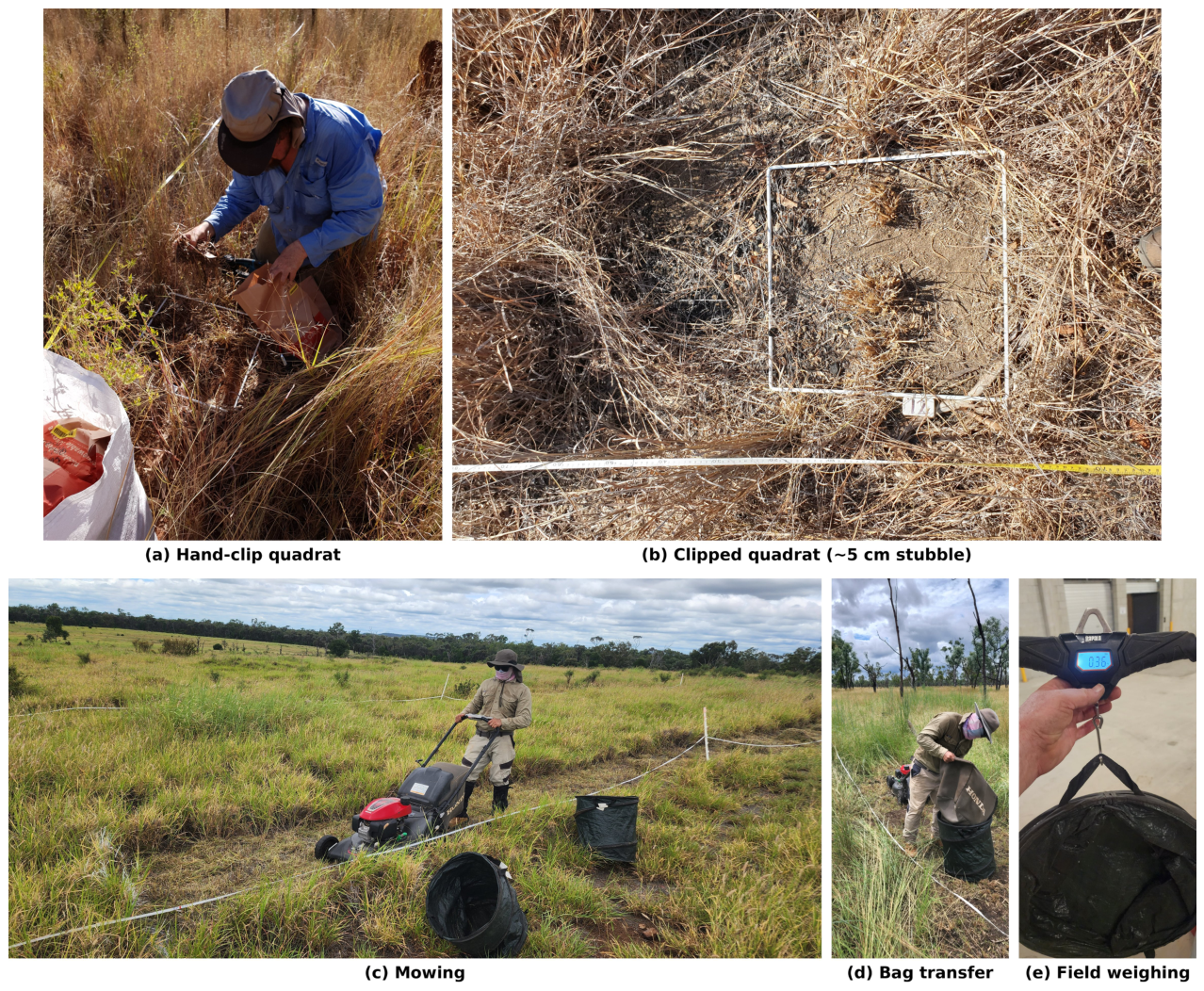
Figure 3.
Example UAV-derived map products at two contrasting field sites. Top row: a managed C4 grassland (Baryugal, bary01, 16 Apr 2024). Bottom row: a grassy-woodland savanna (Mt Pleasant, mtp01, 8 Feb 2024). Columns (where the three-panel layout is rendered): (left) UAV hyperspectral true-colour RGB orthomosaic at the same flight, drawn from the same hyperspectral acquisition described in our companion pasture-chemistry study [22] so the structural pattern in the centre/right panels can be read against a familiar visual context; (centre) 5 cm canopy-height model (DSM minus cloth-simulation DTM); (right) 1 m modelled dry-biomass density from the TabPFN UAV-DSM model with random-forest surrogate, masked to the deep-learning pasture class. The grassland site shows a relatively uniform, dense pasture sward (3–7 t ha−1); the woodland site shows higher mean biomass under partial Eucalyptus overstory (4–10 t ha−1) and a more heterogeneous spatial pattern driven by understory tussock structure. The CHM panels are shown unfiltered: faint orthogonal banding is visible over the mtp01 woodland, an SfM / cloth-simulation-DTM artefact that is amplified by steep crown-edge gradients in timbered areas but averages out at the polygon scale used to train the biomass model.
Figure 3.
Example UAV-derived map products at two contrasting field sites. Top row: a managed C4 grassland (Baryugal, bary01, 16 Apr 2024). Bottom row: a grassy-woodland savanna (Mt Pleasant, mtp01, 8 Feb 2024). Columns (where the three-panel layout is rendered): (left) UAV hyperspectral true-colour RGB orthomosaic at the same flight, drawn from the same hyperspectral acquisition described in our companion pasture-chemistry study [22] so the structural pattern in the centre/right panels can be read against a familiar visual context; (centre) 5 cm canopy-height model (DSM minus cloth-simulation DTM); (right) 1 m modelled dry-biomass density from the TabPFN UAV-DSM model with random-forest surrogate, masked to the deep-learning pasture class. The grassland site shows a relatively uniform, dense pasture sward (3–7 t ha−1); the woodland site shows higher mean biomass under partial Eucalyptus overstory (4–10 t ha−1) and a more heterogeneous spatial pattern driven by understory tussock structure. The CHM panels are shown unfiltered: faint orthogonal banding is visible over the mtp01 woodland, an SfM / cloth-simulation-DTM artefact that is amplified by steep crown-edge gradients in timbered areas but averages out at the polygon scale used to train the biomass model.
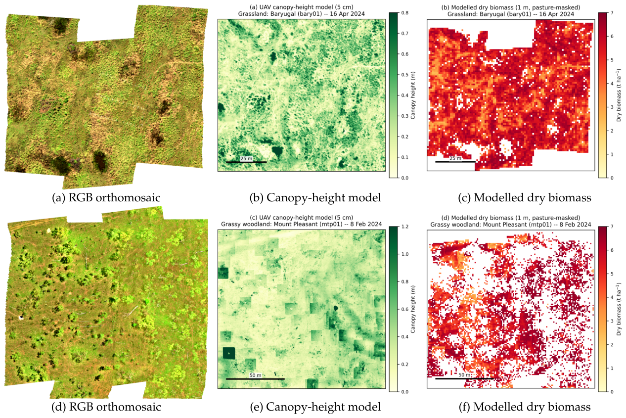
Figure 4.
In-sample observed-versus-predicted scatter for the Sentinel-2 TabPFN biomass model under the three feature configurations (bands-only, bands + NDVI growth, bands + NDVI + TN growth), with embedded cross-validation metrics. Equivalent field- and UAV-scale scatter (mower-swath tare-correction effect, UAV-DSM TabPFN fit) is reported in Appendix F.
Figure 4.
In-sample observed-versus-predicted scatter for the Sentinel-2 TabPFN biomass model under the three feature configurations (bands-only, bands + NDVI growth, bands + NDVI + TN growth), with embedded cross-validation metrics. Equivalent field- and UAV-scale scatter (mower-swath tare-correction effect, UAV-DSM TabPFN fit) is reported in Appendix F.
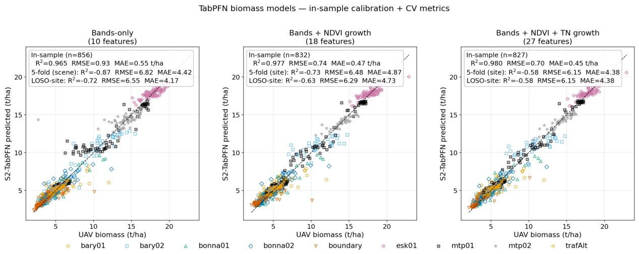
Figure 5.
Operational Sentinel-2 time-series of pasture crude protein (top, derived from leaf-N × 6.25), dry-matter digestibility (second, derived from ADF), dry biomass (third) and daily rainfall with a 30-day rolling total (bottom; Open-Meteo ERA5 reanalysis at the site centroid) over the managed C4 grassland site Baryugal (bary01), 2023-01-01 to 2026-05-10. Solid line = pasture-class mean across 30 pasture pixels within the site footprint; shaded band = inter-quartile range across pixels; vertical dashed line marks the UAV reference flight on 2024-04-16. The black dot on the biomass panel is the site-mean in-situ clip-and-weigh quadrat measurement at that flight (5.47 t ha−1). At the UAV reference date the S2 biomass retrieval (5.26 t ha−1) reproduces both the UAV ground truth (5.22 t ha−1) and the in-situ quadrat mean, and the longer-term retrieval centres on ~5–6 t ha−1 (scene-mean median 5.6 t ha−1 over the 156 cloud-free scenes plotted), with transient high-biomass excursions tracking the post-rainfall growth pulses visible in the bottom panel. Y-axis limits on the chemistry panels are anchored to the site-mean trajectory rather than the across-pixel IQR. Retrievals use the Stage 1 TabPFN biomass model and the TabPFN chemistry models of [22] over 156 cloud-free S2 scenes.
Figure 5.
Operational Sentinel-2 time-series of pasture crude protein (top, derived from leaf-N × 6.25), dry-matter digestibility (second, derived from ADF), dry biomass (third) and daily rainfall with a 30-day rolling total (bottom; Open-Meteo ERA5 reanalysis at the site centroid) over the managed C4 grassland site Baryugal (bary01), 2023-01-01 to 2026-05-10. Solid line = pasture-class mean across 30 pasture pixels within the site footprint; shaded band = inter-quartile range across pixels; vertical dashed line marks the UAV reference flight on 2024-04-16. The black dot on the biomass panel is the site-mean in-situ clip-and-weigh quadrat measurement at that flight (5.47 t ha−1). At the UAV reference date the S2 biomass retrieval (5.26 t ha−1) reproduces both the UAV ground truth (5.22 t ha−1) and the in-situ quadrat mean, and the longer-term retrieval centres on ~5–6 t ha−1 (scene-mean median 5.6 t ha−1 over the 156 cloud-free scenes plotted), with transient high-biomass excursions tracking the post-rainfall growth pulses visible in the bottom panel. Y-axis limits on the chemistry panels are anchored to the site-mean trajectory rather than the across-pixel IQR. Retrievals use the Stage 1 TabPFN biomass model and the TabPFN chemistry models of [22] over 156 cloud-free S2 scenes.
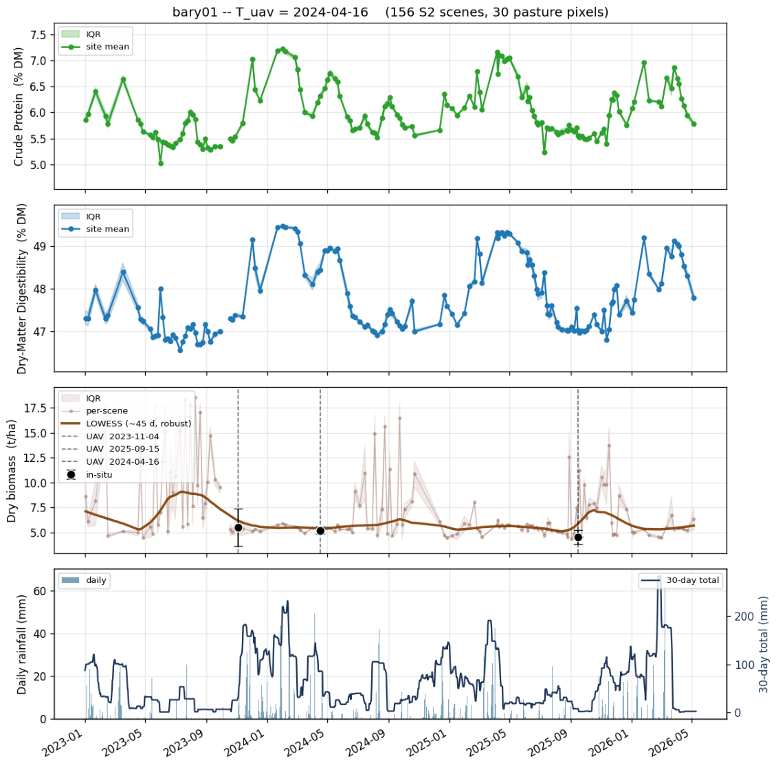
Table 1.
Vegetation groups and dominant species sampled at each property.
| Property | Vegetation group | Dominant species |
|---|---|---|
| Property A – Trafalgar (Sites 1–2) | Woodland | Native / Naturalised grasses, shrubs |
| Property A – Trafalgar (Site 3) | Grassland | Native / Naturalised grasses |
| Property B – Mt Pleasant (Sites 1–2) | Woodland | Native grasses, shrubs, trees |
| Property C – Bon Accord (Sites 1–2) | Grassland | Native / Naturalised grasses |
| Property D – Baryugal (Sites 1–2) | Grassland | Native / Naturalised grasses |
| Property E – Esk (Sites 1–2) | Grassland / Woodland | Native / Naturalised grasses |
Table 2.
Cross-validation of the combined-geometry UAV-DSM TabPFN biomass model. n=489 polygon-level samples across 17 site-date groups; n_groups reports the number of groups in the spatial CV split.
Table 2.
Cross-validation of the combined-geometry UAV-DSM TabPFN biomass model. n=489 polygon-level samples across 17 site-date groups; n_groups reports the number of groups in the spatial CV split.
| Split | n | RMSE (t ha-1) | MAE (t ha-1) | R2 |
|---|---|---|---|---|
| in-sample | 489 | 1.74 | 1.21 | 0.938 |
| 5-fold (site, date) | 489 | 6.74 | 4.09 | 0.073 |
| LOSO-site | 489 | 8.10 | 4.94 | −0.339 |
| LOSO-site-date | 489 | 8.06 | 4.95 | −0.326 |
Table 3.
Cross-validation of the three Sentinel-2 TabPFN biomass models.
| Model | Split | n | RMSE (t ha-1) | MAE (t ha-1) | R2 |
|---|---|---|---|---|---|
| Stage 1: Snapshot 10-band | in-sample | 856 | 0.68 | 0.42 | 0.978 |
| 5-fold | 856 | 3.87 | 2.38 | 0.307 | |
| LOSO-site | 856 | 3.97 | 2.45 | 0.270 | |
| Stage 2: NDVI growth | in-sample | 641 | 0.63 | 0.42 | 0.979 |
| 5-fold | 641 | 4.19 | 3.04 | 0.042 | |
| LOSO-site | 641 | 4.14 | 2.90 | 0.069 | |
| Stage 3: NDVI + TN growth | in-sample | 500 | 0.59 | 0.41 | 0.977 |
| 5-fold | 500 | 3.95 | 2.88 | −0.025 | |
| LOSO-site | 500 | 3.70 | 2.47 | 0.104 |
Table 4.
Aggregate-level leave-one-site-out cross-site generalisation ( site-date aggregates, 9 sites; back-transformed predictions). RMSE units are . Bold cell highlights the best LOSO .
Table 4.
Aggregate-level leave-one-site-out cross-site generalisation ( site-date aggregates, 9 sites; back-transformed predictions). RMSE units are . Bold cell highlights the best LOSO .
| Feature set | Learner | 5-fold | LOSO | LOSO RMSE | LOSO MAE |
|---|---|---|---|---|---|
| Spectral only (27) | GBM | 4.79 | 2.96 | ||
| TabPFN | 4.57 | 3.23 | |||
| Stack | 4.54 | 2.99 | |||
| Spectral + environmental (42) | GBM | 4.32 | 2.68 | ||
| TabPFN | 4.79 | 3.25 | |||
| Stack | 4.50 | 2.84 | |||
| Environmental only (15) | GBM | 2.51 | |||
| TabPFN | 4.63 | 3.05 | |||
| Stack | 4.36 | 2.65 |
Disclaimer/Publisher’s Note: The statements, opinions and data contained in all publications are solely those of the individual author(s) and contributor(s) and not of MDPI and/or the editor(s). MDPI and/or the editor(s) disclaim responsibility for any injury to people or property resulting from any ideas, methods, instructions or products referred to in the content. |
© 2026 by the authors. Licensee MDPI, Basel, Switzerland. This article is an open access article distributed under the terms and conditions of the Creative Commons Attribution (CC BY) license (http://creativecommons.org/licenses/by/4.0/).
Copyright: This open access article is published under a Creative Commons CC BY 4.0 license, which permit the free download, distribution, and reuse, provided that the author and preprint are cited in any reuse.


