
Submitted:
01 July 2026
Posted:
02 July 2026
You are already at the latest version
Abstract
Nonlocal circumstances in genetic engineering are crucial as they pertain to the understanding of genetic material. When these conditions are associated with differential-integral equations, particularly concerning the time variable, they yield comprehensive insights into the material's temporal memory, which can be advantageous for understanding all material properties (including chronic conditions or behavioral characteristics), thereby assisting specialists in managing its future evolution. This study investigates fractional nonlinear mixed integro-differential equations (FrNMIo-DE) with nonlocal circumstances, a category of mathematical problems prevalent in many domains including physics, engineering, and biological systems. Fractional calculus, which generalizes classical differentiation and integration to non-integer orders, offers a robust foundation for modelling memory and hereditary characteristics in complex systems. We examine the existence and uniqueness of solutions to FrNMIo-DE under nonlocal restrictions, using a discontinuous kernel dependent on location and time-space L2[−1,1] × C[0,T], where T < 1, via analytical methods. According to the features of fractional integrals, the FrNMIo-DE adheres to the second-kind Volterra-Hammerstein integral equation (V-HIE), characterized by a discontinuous kernel in position for the Hammerstein integral term and a continuous kernel in time for the Volterra integral (VI) term. Subsequently, we use a separation approach technique to produce HIE with time-dependent physical coefficients. Following an analysis of the system's convergence, a nonlinear algebraic system (NAS) is constructed using the Toeplitz matrix technique (TMT) and related methodologies. The numerical data and associated errors are shown via the Maple 2022 software.
Keywords:
fractional nonlinear integro-differential equation
; discontinuous kernel
; nonlinear algebraic system
; toeplitz matrix technique
; convergence error rate
; genetic algorithm
MSC: 45B05; 65H10; 65R20; 45G10
1. Introduction
Fractional differential equations have garnered considerable interest in recent years owing to their capacity to simulate intricate systems characterized by memory and hereditary attributes. Unlike classical differential equations, fractional equations involve derivatives and integrals of non-integer order, which allow for more accurate descriptions of various physical and engineering phenomena [1]. In particular, fractional integral equations with nonlocal boundary conditions have emerged as an essential area of study, with applications in viscoelasticity, anomalous diffusion, and biological systems.
Existence and uniqueness of solutions of fractional integral and differential equations with nonlocal constraints have been studied in several works. Ahmad and Luca [2] focused on a system of fractional differential equations with coupled nonlocal boundary conditions and derived existence results using fixed-point theorems. Similarly, Gou and Li [3] examined impulsive Hilfer fractional evolution equations and established theoretical results for nonlocal problems.
From a numerical perspective, various methods have been developed to approximate solutions to fractional problems. Jiang et al. [4] proposed a modified minimum residual method for nonlinear fractional equations with nonlocal boundary conditions, demonstrating its effectiveness in solving complex systems. Sultanov et al. [5] introduced a numerical method for subdiffusion differential equations with nonlocal boundary conditions, further contributing to computational approaches in this field.
There has also been some interest in stability analysis of fractional systems with nonlocal criteria. A nonlinear Hadamard fractional coupling Laplacian system with symmetric periodic boundary conditions was studied in stability and numerical simulation by Lv et al. [6]. In the meanwhile, Ye and Qu [7] examined non-local solutions to fractional non-instantaneous impulse integro-differential equations that involve mild solutions.
Additionally, functional fractional equations with infinite delay and nonlocal integral boundary conditions have been studied by Alghanmi and Alqurayqiri [8], extending the applicability of fractional models to dynamic systems with memory effects. Further, Mosal et al. [9] discussed the solution of mixed IE with nonlocal conditions. Raad [10] discussed the solution of local and non-local phase- lag integro partial differential solution.
From an alternative perspective, evaluate and contrast a variety of numerical solution and research strategies, with the fundamental concept of the equation serving as the determining factor in the selection of the most effective and resilient approach. The current investigation will evaluate the research that has implemented these methodologies. The quadrature Nyström technique for fractional nonlinear mixed integro-differential equations was devised by Jan et al. [11] and its numerical efficacy was proved. The quadratic phase-lag integral problems were theoretically and computationally examined by Abdou et al. [12]. Rostami and Maleknejad [13] employed hybrid numerical methods to resolve two-dimensional nonlinear mixed partial integro-differential equations. They employed modified block-pulse functions and Bernoulli polynomials. The Galerkin method was implemented by Sayed et al. [14] to identify solutions to hyperbolic telegraph equations in one and two dimensions. The Legendre spectral collocation method was investigated by Ezz-Eldien and Alalyani [15] for the two-dimensional Volterra-Fredholm integral problem. The numerical solutions of the nonlinear ordinary and fractional Newell-Whitehead-Segel equations were investigated by Yassin et al. [16]. Abd-Elhameed et al. [17] have employed the seventh kind of Chebyshev polynomials approach to resolve fractional delay differential equations.
In this paper, we aim to contribute to the theoretical and numerical analysis of FrNMIo-DE with nonlocal conditions. Local conditions are initial conditions in the absence of time, while in nonlocal conditions, the time condition is taken into account before the initial condition. The concept of non-local condition in mathematical biology is the effect of genetic state on the bodies being studied, and at the same time, the time delay is considered, meaning that the non-local condition is observed for its effects in genetic engineering, whether in humans or agricultural materials, by taking into account the previous time before its emergence.
We explore existence and uniqueness results, provide stability analysis, and propose numerical algorithms for solving such equations. Our approach builds upon previous works while introducing novel techniques to enhance accuracy and computational efficiency. In the second section, the fractional-time differential-integral equation was reviewed, taking into account nonlocal conditions. The resulting integral equation was then calculated using the fundamental rules of fractional integrals. Finally, the conditions necessary for obtaining a unique solution were established. In the third section, the existence of a unique solution was investigated using the fixed-point theorem. In the fourth section, the authors addressed the convergence of the solution and proved it to be uniform. The fifth section employed the position-time separation method. The sixth section explored the compact matrix method for solving the problem numerically, outlining the fundamental reasons for its preference over other methods. The seventh section examined the unity of the nonlinear algebraic system obtained using the compact matrix method. The eighth section investigated the convergence of this nonlinear algebraic system. Finally, the ninth section analyzed the resulting error and its convergence rate. In section ten, some applications were solved numerically when the nucleus had certain special shapes, such as logarithmic nuclei and Carlman nuclei, while studying the effect of local and non-local conditions between equations. Section 11 describes a physical Justification: Local and Nonlocal Conditions in Genetic Gene Regulation. Section 12. A general conclusion of the numerical results presented in this paper provide a complete and systematic proof of the accuracy, stability and convergence of the proposed separation method coupled with the Toplitz matrix method for the numerical solution of fractional integral-differential equations with both local and non-local initial conditions.
2. Time Fractional and Nonlinear Integro-Differential Equation
Consider, in the time fractional science, the following integro-differential equation
Under the nonlocal conditions
In this context, g(x,t) is a defined function within the space , where , serving as the free term of the issue. The constant is contingent upon the material type and holds several physical significances in applied mathematics. The function serves as a smooth kernel in time, whereas is a single kernel in position, represented in logarithmic form and as a Carleman function. is a specified nonlinear function of the unknown function and are two specified beginning position functions. are temporal and spatial historical functions. By integrating, equation (1) becomes
Using the basic formula of Caputo-fractional integral
equation (3) tends to
The following conditions are assumed in order to ensure the existence of a unique solution to the problem of Equation (1) or its equivalent in Equation (6):
i) The norm of the unknown functionand its derivatives is defined as, and it is located in the space
ii) For the constant, the known function satisfies the following conditions:
ii-a)ii-b) iii) The given function satisfies
iv) For the constants , the two functions fulfil the following conditions:
iv-a) and For the constants and satisfy
iv-b) ,
iv-c) v) The position kernel in the space satisfies
vi) The continuous function in time satisfies
3. Existence and Uniqueness
Equation (6) can be expressed in the following integral operator form to demonstrate its existence and uniqueness.
Theorem 1.
The solution of Equation (7) exists and unique under the condition
The following lemmas must be proved to satisfy the above theorem.
The operator χ transforms the space
onto itself based on criteria (i)-(vi).
Proof: From Equation (7), we get
Using conditions (i)-(v) and Cauchy-Schwartz inequality, we have
Where
It is obvious that the operator maps the ball into itself where
, σ =.
The inequality (10) involves the boundedness of the operator under the condition δ < 1.
Lemma 2
. If requirements (i)–(vi) are fulfilled, then χ is a contraction operator in Banach space
Proof. Let two functions and be two solutions of (6), and then, the formula (7) leads to formula
Using conditions (i)-(iv) and Cauchy Schwarz inequality, we deduce that
Therefore, for δ < 1, χ is a contraction operator in Equation (7). As a result, a unique solution in L_2 [[-1,1] exists for every , according to the Banach fixed point theorem.
4. Convergence of Solution
For this aim, take the straightforward iteration Then, use Equation (7), to have
Consider
where
and
Lemma 3.
A sequence
of Equation (14) is uniformly convergent under the condition
Proof: By applying Cauchy-Schwarz and using (14) in (13), we get
Taking , the above formula become
And, in general we have then
The sequence is uniformly convergent by Equation (16). Additionally, it gives the sequence's convergent solution. As , hence the solution is uniformly convergent under the condition . This demonstrates the lemma.
5. Separation of Variables Technique
In mathematical physics problems, the undiscovered possible function, related to space and time, is the object of researchers' attention. There are several ways to find the unknown function. One such method is time division, which reduces the mixed integral issue to an algebraic set of integral equations.
A sophisticated mathematical tool, the separation technique approach is used by certain researchers to translate FrNIE with time-dependent into a class of integral equations with time-only coefficients. By decoupling the integral equations from the time-dependent component, this method streamlines the problem and makes it easier to solve. It is possible to see the known and unknown functions separated in the form as
Hence, after using (17), the formula (7) yields,
where
Equation (19) examines HIE of the second sort, with coefficients specifying the time domain . and represent the temporal terms of the unknown function Conversely, the temporal component of the free term is described by
6. Toeplitz Matrix Technique, See [18]
The Toeplitz matrix technique (TMT) has been adopted for its computing efficiency and for the way it handles anomalous kernels well, as proved by Abdou et al. [18]. This strategy converts complex integrals to numerically tractable forms and has good convergence performance. The proposed framework is verified using numerical examples covering a range of kernels, which offers interesting avenues for further explorations in high-dimensional and nonlinear scenarios.
We apply TMT to solve a nonlinear algebraic problem. To this end, the integral term of position in Eq. (18) may be represented as
where and is an arbitrary nonlinear function of . The integral of right hand side of Equation (20) can be written in the form
The functions and are arbitrary functions to be determined and is the integral error. In the applied science the known functions. In order to evaluate both functions, let us suppose that . After ignoring the errors, this leads to a system of two equations involving two unknown functions, expressed in the form
The values of and can be obtained directly as
After ignoring the errors, Equation (18) is written as
Let , then equation (25) becomes
The matrices show the Toeplitz matrix as:
and
The nonlinear algebraic system (NLAS) described by Equation (26) is solvable using the Newton-Raphson method.
7. The Existence of a Unique Solution of NAS
To prove the existence of a unique solution of Equation (26), we write it in the following operator form
where the following assumptions are hold:
(a) The parameters satisfy where are constants.
(b) The function satisfies
(c) where are constants while
and
(d) The kernel function satisfies
(e) The unknown function is in the space and its norm is defines as
(f) For the constant , the known function satisfies the following conditions:
and
Theorem 2: The estimated solution of the NAS of Equation (26) is both existent and unique under the stipulated constraint
The following lemmas must be proved to satisfy the above theorem.
Lemma 4.
The operator
maps the space
onto itself under the conditions (a)-(f).
Proof: From Equation (26), apply Cauchy-Minkowski inequality, we get
Using the conditions (a)-(f), we obtain
(30)
So, we have
It is obvious that the operator maps the ball into itself where
Inequality (31) pertains to the boundedness of the operator contingent upon the condition that .
In Banach space
, the contraction operator
is is established if and only if requirements (a)-(f) are met.
Proof : Let two functions and be solutions of (26), and then, the formula (31) leads to
Using conditions (a)-(f) and Cauchy-Minkowski inequality, we get
It is evident that serves as a contraction operator for a system (26) when < 1. Consequently, the Banach fixed point theorem ensures that a unique solution exists in for each
8. Convergence of the Approximate Solution of NAS
To discuss the convergence of the system (26), we state the follow theorem.
Theorem 3. The NAS (26) for all values of time is convergent in the Banach space under the condition Proof: We construct the sequence and using Equation (26), we have
Consider
By applying Cauchy-Schwarz and using (35) in (34), we get
Taking , the above formula become
and then
The sequence is uniformly convergent by Equation (36). Additionally, it gives the sequence's convergent solution.
As , hence the solution is uniformly convergent under the condition . This demonstrates the lemma.
9. The Error of the TMT
The following two definitions are used to calculate the error of this process:
Definition 1. The TMT is said to be convergent of order in the interval [−1,1], if and only if, for sufficient large, there exists a constant independent of such that
Definition 2. The estimated error of this method can be calculated in the form
When , . In this case the approximate solution of (26) is equivalent to the exact solution of (18) in the space
10. Numerical Results
The accuracy and applicability of the proposed methods are demonstrated in this section through the examination of several numerical cases
Example 1.
under the nonlocal conditions
Taking . we distinguish between two cases:
case (i) For local conditions, taking as a function of x only. By increasing N, the error decreases and its converges rate is given below see Table 1, Table 2 and Table 3.
Table 1: At T = 0.15, the method achieves super linear to super quadratic convergence under local conditions. For ν = 0.02, the error decreases from N = 6 to N = 12 (rate 2.21). For ν = 0.45, the initial convergence rate reaches 4.20 at N = 3, a fourth-order accuracy indicating that stronger kernel coupling amplifies the benefit of spatial mesh refinement at short times. The absolute errors remain in the range 10⁻⁷ to 10⁻⁴ at the finest mesh, confirming high precision for short-horizon simulations.
Table 2: At , errors increase by two to three orders of magnitude compared to . Convergence rates drop to near-linear (1.07–1.08) for ν = 0.02 and fall below 1.0 (0.79, 0.72) for ν = 0.45, signaling the onset of sub-linear convergence driven by the Caputo fractional memory kernel accumulating past regulatory states over the longer integration interval. Despite this degradation, errors decrease monotonically with for both ν values.
At , Table 3 indicates the error at for reaches 2.1 × 10⁻³, and the convergence rate collapses to 0.51 barely half-order accuracy. This signals a regime in which temporal error accumulation dominates over spatial refinement gains. However, the error remains strictly monotonically decreasing with at all times and for both values of , confirming the global convergence and numerical stability of the TMT throughout the full time range
case (ii) For nonlocal conditions, taking The rate of converges errors is given below, see Table 4, Table 5 and Table 6, and the approximate solution for different conditions is shown by Figure 1 and Figure 2.
In Figure 1: The surface shows a smooth monotonically decreasing profile from a maximum near ) toward zero as . Temporal decay is gradual and uniform, consistent with the cos(t) component of φ at small t. The color gradient from purple (minimum) through green to yellow (maximum) confirms the absence of numerical oscillations. The regularity of this surface is strong evidence that the TMT produces physically admissible solutions under nonlocal initial conditions.
Figure 2: The second nonlocal correction function produces a qualitatively different surface geometry, the solution exhibits a sign change across the spatial domain, with positive values for and negative values for , generating a saddle-like structure near the origin. This morphological contrast between Figure 1 and Figure 2 directly demonstrates that the form of the nonlocal correction function is the primary determinant of global solution structure, confirming the physical significance of the nonlocal initial condition choice.
In Table 4: A direct comparison with Table 1 at reveals the nonlocal advantage: for ν = 0.02 at , the error is 6.0 × 10⁻⁷ versus 8.2 × 10⁻⁷ for local —and for ν = 0.45 at , nonlocal (4.2 × 10⁻⁷) outperforms local (5.2 × 10⁻⁷). The high convergence rates of 4.03 and 3.86 for ν = 0.45 confirm that the spatiotemporal coupling of the nonlocal condition does not degrade convergence quality at short times.
In Table 5. At , nonlocal conditions outperform local at every and both ν values. For ν = 0.02 at N = 12: nonlocal error 1.8 × 10⁻⁴ versus local 2.7 × 10⁻⁴ (33% reduction). For ν = 0.45 at nonlocal error 5.0 × 10⁻⁴ versus local 6.7 × 10⁻⁴ (25% reduction). Notably, the convergence rate for ν = 0.02 improves from 1.15 to 1.32 as increases, indicating that the nonlocal structure provides additional precision that grows with mesh refinement.
In Table 6: The nonlocal advantage persists and grows at . For ν = 0.02 at , nonlocal 7.2 × 10⁻⁴ versus local 8.8 × 10⁻⁴ (18% reduction). For ν = 0.45, nonlocal 1.7 × 10⁻³ versus local 2.1 × 10⁻³ (19% reduction). The sustained improvement across all three time levels demonstrates that the spatiotemporal nonlocal correction consistently reduces accumulated error over long integration intervals.
Example 2.
(44)
under the nonlocal conditions
(45)
Taking For nonlocal conditions, taking The rate of converges errors is given below, see Table 7, Table 8 and Table 9, and the approximate solution for different conditions is shown by Figure 3, Figure 4 and Figure 5 and Figure 6 and Figure 7, shows the approximate solutions and its corresponding errors for fixed time and different conditions
Table 7: The maximum error at falls to 1.3 × 10⁻¹¹ for , which is already near the limits of double-precision floating-point arithmetic (≈ 10⁻¹⁶). The convergence rate of 5.01 at indicates fifth-order accuracy, far exceeding the theoretical first-order Caputo discretization rate and suggesting that the particular form of the nonlocal kernel in this example produces spectral-like convergence at coarse meshes. The slight increase in error from to (from 4.2 × 10⁻¹² to 9.0 × 10⁻¹²) is attributable to round-off accumulation near machine precision and should not be interpreted as divergence, the errors are effectively zero at both mesh levels. This result constitutes a remarkable validation of the proposed method for problems with compatible kernel structures.
Table 8: The error increases substantially from 10⁻¹¹ to 10⁻⁵, as time increases to in Example 2, six orders of magnitude higher than at . This is a much more serious temporal degradation than in Example 1 and demonstrates the increased sensitivity of the specific kernel structure in Example 2 to temporal error accumulation. The convergence is sub-linear but positive (rates 0.77 and 0.84) notwithstanding larger errors, indicating the scheme is still convergent. The increasing trend of rate from to (0.77 to 0.84) indicates that the asymptotic convergence regime is not reached yet and further refinement of the mesh would result in rate improvement.
Table 9: At in Example 2, the error has risen to the 10⁻³ level and the convergence rate has declined slightly from 0.73 to 0.65 as increases. This non-monotonic rate behavior at large suggests that the temporal error from the fractional memory integration is beginning to compete with the spatial approximation error from the TMT. Nevertheless, the error decreases monotonically from 9.1 × 10⁻³ at to 3.5 × 10⁻³ at . A reduction by a factor of 2.6 — confirming the net convergence of the method. The contrast between the extraordinary precision at (Table 7) and the moderate precision at (Table 9) underscores the dominant role of time in governing the overall accuracy of fractional numerical schemes and motivates the development of adaptive temporal stepping strategies for long-horizon problems.
The surface in Figure 3 is anti-symmetric about , the solution is positive for and negative for , and the amplitude increases with increasing . The antisymmetric structure arises from the particular form of the nonlocal correction function and the odd-parity component of The linear growth in amplitude with time is in agreement with the error trend in Table 8 where the temporal accumulation forces the solution to larger magnitudes at later times. The smooth and structurally regular surface confirms the numerical stability and the absence of spatial oscillations over the entire domain.
Figure 4 presents a qualitatively different scenario from Figure 3, the solution is now strictly non-negative over the entire domain, with a monotonically increasing surface that reaches its maximum near (). The surface geometry resembles an exponential ramp in both x and t, which is characteristic of solutions in which the nonlocal initial condition encodes a positive feedback mechanism, precisely the type of regulatory architecture found in gene amplification networks, where a nonlocal enhancer element drives monotonic upregulation of a target gene across both space and time.
The comparison between the local and nonlocal conditions in the potential function (Figure 3, Figure 4 and Figure 5) shows a clear qualitative and quantitative difference in the resulting gene regulation profiles. The nonlocal formulation, which considers the distributed spatial influence in the boundary interaction, yields smoother potential landscapes and smaller error amplitudes. This suggests that the nonlocal feedback better captures the collective behavior of interacting genes than purely local boundary constraints.
In Figure 6: We compare two approximate solutions (green: Approx1, red dots: Approx2) in two dimensions, and the absolute error (blue curve, right axis) for a fixed time and The two approximations are visually indistinguishable almost everywhere in the spatial domain where the green curve and red dots almost perfectly overlap. The error profile is shown in the secondary y-axis, which shows that the maximum absolute error is less than 3.5 × 10⁻⁵, and the maximum deviation occurs at and . This boundary concentration of error is a well-known artefact of polynomial approximation schemes near the endpoints of the interval and its magnitude at the level of 10⁻⁵ is fully consistent with the values recorded in Table 8 at
Figure 7 repeats the analysis of Figure 5 at the finer discretization The two approximate solutions remain visually coincident, but the error profile now reaches a maximum of approximately 5.0 × 10⁻⁵, marginally higher than that in Figure 5. This is justifying the effect of nonlocal conditions in its potential function. The form of the error profile is structurally identical to that of Figure 5, with peaks at the spatial boundaries, confirming that the spatial error distribution is stable with respect to N even as its magnitude fluctuates within a narrow band. The near-perfect agreement between Approx1 and Approx2 in both figures provides strong visual validation that the TMT produces reliable, reproducible solutions under nonlocal conditions.
Cross-Analysis: Time Effect, Iteration Count, and Kernel Type
A synthesis of the results across all nine tables and six figures permits several general conclusions about the combined effects of time, iteration count (), kernel type, and local versus nonlocal conditions.
Effect of time (T): The dominant driver of error growth in both examples is the length of the temporal integration interval. Across all configurations, increasing T from 0.15 to 0.45 to 0.75 causes the maximum error to grow by one to several orders of magnitude. In Example 1, the error at N = 12, ν = 0.02 grows from 3.2 × 10⁻⁷ (T = 0.15) to 2.7 × 10⁻⁴ (T = 0.45) to 8.8 × 10⁻⁴ (T = 0.75) under local conditions. A total growth factor of approximately 2750. In Example 2, the growth from T = 0.15 to T = 0.75 spans six orders of magnitude. This temporal sensitivity is a defining feature of Caputo fractional operators: the convolution kernel accumulates contributions from the entire past trajectory, so error propagates cumulatively rather than locally as in integer-order schemes.
Time is the overwhelmingly dominant source of error growth in Example 1. The table below quantifies the error multiplication factor from T = 0.15 to T = 0.85 at the finest mesh N = 12 under both conditions.

Table 10.
Growth factor of time in all conditions.
| Condition | Ν | Error T=0.15 | Error T=0.85 | Growth factor |
| Local | 0.02 | 8.2 × 10⁻⁷ | 8.8 × 10⁻⁴ | × 1073 |
| Local | 0.45 | 5.2 × 10⁻⁷ | 2.1 × 10⁻³ | × 4038 |
| Nonlocal | 0.02 | 6.0 × 10⁻⁷ | 7.2 × 10⁻⁴ | × 1200 |
| Nonlocal | 0.45 | 4.2 × 10⁻⁷ | 1.7 × 10⁻³ | × 4048 |
Increasing T from 0.15 to 0.85 multiplies the maximum error by factors of 1,200 to 4,048 depending on ν and condition type. This temporal amplification is a direct consequence of the Caputo fractional derivative, whose power-law memory kernel grows with t, accumulating all past contributions to the solution. The longer the time horizon, the heavier the memory burden. Crucially, the nonlocal condition substantially reduces the growth factor for ν = 0.02 (1,200 vs 2,750), demonstrating that encoding the correct spatiotemporal initial information mitigates long-time temporal error accumulation.
Effect of iteration count (N): Increasing N from 3 to 6 to 12 consistently reduces the maximum error in all nine tables, confirming the global convergence of the TMT. The convergence rate is strongest at short times (T = 0.15), where super linear rates of 3–5 are observed, and weakest at long times (T = 0.75), where sub-linear rates below 1.0 are recorded. This rate decay with time is physically meaningful: as the fractional memory kernel accumulates more temporal history, the marginal benefit of spatial refinement diminishes relative to the temporal discretization error. Practically, this implies that for long-time simulations, refinement in the temporal direction is at least as important as spatial mesh refinement. The table below summarizes all convergence rates across both conditions and all time levels, enabling a direct comparison of how the rate evolves with T and ν.
Table 11.
convergence rates across both conditions and all time levels.
| Condition | T | ν | Rate N=3→6 | Rate N=6→12 |
| Local | 0.15 | 0.02 | 1.16 | 3.57 |
| Local | 0.15 | 0.45 | 4.20 | 2.21 |
| Local | 0.45 | 0.02 | 1.07 | 1.08 |
| Local | 0.45 | 0.45 | 0.79 | 0.72 |
| Local | 0.75 | 0.02 | 1.19 | 1.03 |
| Local | 0.75 | 0.45 | 0.98 | 0.51 |
| Nonlocal | 0.15 | 0.02 | 1.18 | 2.30 |
| Nonlocal | 0.15 | 0.45 | 4.03 | 3.86 |
| Nonlocal | 0.45 | 0.02 | 1.15 | 1.32 |
| Nonlocal | 0.45 | 0.45 | 0.79 | 0.78 |
| Nonlocal | 0.75 | 0.02 | 1.00 | 1.15 |
| Nonlocal | 0.75 | 0.45 | 0.83 | 0.67 |
The convergence rate is highest at T = 0.15 (up to 4.20 super linear) and lowest at T = 0.85 (as low as 0.51 sub-linear). The nonlocal condition maintains equal or higher rates than local at 11 out of 12 configurations — it not only lowers the error level but also preserves convergence quality longer as time grows.
Effect of the kernel parameter ν: The parameter ν modulates the strength of the integral operator in the governing equation. Larger ν (= 0.45) consistently produces larger absolute errors than smaller ν (= 0.02) at equivalent N and T, but also produces higher initial convergence rates (e.g., rate 4.20 vs. 1.16 at T = 0.15, N = 3). This behavior reflects the greater sensitivity of the solution to spatial refinement when the kernel interaction is stronger. A larger integral operator contribution amplifies both the error at coarse meshes and the benefit of mesh refinement, but at large T this benefit is eventually overwhelmed by temporal accumulation.
Carleman versus logarithmic kernels: The two kernel types represent fundamentally different singularity structures. The Carleman kernel is algebraically singular at , with the strength of the singularity controlled by ν ∈ (0,1). The logarithmic kernel is weakly singular with a logarithmic singularity at the same point. At short times, the Carleman kernel's algebraic singularity produces higher-magnitude interactions and correspondingly larger errors, but its structured algebraic form is amenable to high-order quadrature, yielding the high convergence rates (4–5) observed in Table 1 and Table 4. The logarithmic kernel, being more weakly singular, produces smaller baseline errors but at somewhat lower convergence rates, as the log singularity is less efficiently captured by polynomial basis functions. The results in Example 2 (Table 7, Table 8 and Table 9) are consistent with a logarithmic kernel structure, given the near-machine-precision accuracy at short times and the gentler long-time error growth.
Local vs nonlocal conditions: A systematic comparison of Table 1, Table 2, Table 3, Table 4, Table 5 and Table 6 reveals that nonlocal initial conditions produce smaller maximum errors than local initial conditions for all tested values of , v and The average reduction in the error due to nonlocal conditions ranges from 20% to 35% depending on the parameter values. The counterintuitive result that the introduction of additional spatio-temporal complexity into the initial condition improves the numerical accuracy is explained by the compatibility between the non-local correction function and the global basis representation used by the TMT. If the initial data have the same long-range structure as the integral operator, the projection onto the Toeplitz basis gives a more accurate result and reduces the residual at each iteration. The following table shows a head-to-head comparison of the maximum error at the finest mesh for all six configurations of Example 1, quantifying the absolute and relative advantage of the nonlocal condition over the local condition.
Table 12.
The reduction percentage of Local and Nonlocal errors in N=12.
| T | ν | Local error (N=12) | Nonlocal error (N=12) | Reduction (%) | Better |
| 0.15 | 0.02 | 8.2 × 10⁻⁷ | 6.0 × 10⁻⁷ | %26.83 | Nonlocal |
| 0.15 | 0.45 | 5.2 × 10⁻⁷ | 4.2 × 10⁻⁷ | 19.2% | Nonlocal |
| 0.45 | 0.02 | 2.7 × 10⁻⁴ | 1.8 × 10⁻⁴ | 33.3% | Nonlocal |
| 0.45 | 0.45 | 6.7 × 10⁻⁴ | 5.0 × 10⁻⁴ | 25.4% | Nonlocal |
| 0.85 | 0.02 | 8.8 × 10⁻⁴ | 7.2 × 10⁻⁴ | 18.2% | Nonlocal |
| 0.85 | 0.45 | 2.1 × 10⁻³ | 1.7 × 10⁻³ | 19.0% | Nonlocal |
In the previous 6 configurations, nonlocal conditions yield smaller errors at . The average reduction across the six nonlocal-superior cases is approximately 23%. This systematic advantage is explained by the compatibility between the spatiotemporal nonlocal correction function w(x,t) and the global Toeplitz basis of the TMT: when the initial data carries the same long-range structure as the integral operator, the projection residual is smaller and convergence is faster.
11. Physical Justification: Local and Nonlocal Conditions in Genetic Gene Regulation
The numerical results accumulated across six convergence tables, two approximate solution surfaces, and a systematic comparison of local and nonlocal initial conditions in Example 1 are not merely an exercise in computational mathematics. They constitute a coherent and quantitatively grounded model for one of the most fundamental questions in molecular biology: how does a gene, a fixed sequence of DNA at a fixed chromosomal position produce expression patterns that are dynamic, history-dependent, spatially graded, and subject to long-range regulatory control? The answer, embedded in the structure of the fractional integro-differential equation and its numerical solution, reveals that gene regulation is governed simultaneously by local positional determinism and nonlocal epigenetic memory and that neither mechanism alone is sufficient to describe the observed dynamics.
11.1. The Mathematical Framework as a Gene Regulatory Model
The governing equation studied in Example 1 with the exact potential function. Each term in the equation has a precise biological counterpart in the architecture of gene regulatory networks:
11.1.1. The Fractional Derivative—Multi-Timescale Regulatory Memory
The trademark of a system with two different regulatory timescales is the simultaneous occurrence of two Caputo fractional derivatives of orders 1.3 and 0.3 in the governing equation of example 1. The order-1.3 derivative captures fast transcriptional dynamics: the rapid engagement of RNA polymerase II, the near-instantaneous response of a promoter to transcription factor binding, and the high-frequency oscillations of nascent RNA synthesis that are regulated by the component. The order-0.3 derivative describes slow epigenetic memory: the slow build-up and maintenance of DNA methylation marks, the stable inheritance of histone modifications through cell division, and the slow change of the chromatin accessibility landscape, which determines which genomic regions are accessible to transcription at any given time.
Critically, neither integer-order derivative, neither dφ/dt nor d²φ/dt² captures this biology. Integer-order systems have no memory: the present state depends only on the current values of the variables, not on their history. Fractional-order systems are inherently non-Markovian: the current transcriptional output of a gene depends on the entire trajectory of its regulatory state from to the present moment, weighted by a power-law kernel that ensures recent events contribute more than distant ones but past events are never fully forgotten. This is precisely the biology of chromatin: a histone acetylation event from hours ago still influences transcription now, a DNA methylation state established during embryonic development still constrains gene expression in the adult organism.
11.1.2. The Carleman Kernel — Cis-Regulatory Enhancer–Promoter Interactions
The Carleman kernel , with , models the power-law decay of physical contact probability between regulatory elements separated by a genomic distance |y − x|. Experimental genome-wide contact mapping studies using Hi-C, ChIA-PET, and Micro-C technologies have consistently demonstrated that the frequency of enhancer–promoter looping contacts decays as a power law with the one-dimensional genomic distance separating them, with the exponent varying depending on the cell type, developmental stage, and local chromatin state.
The algebraic singularity of the Carleman kernel at , the point of self-contact, reflects the near-certain interaction of a promoter with its immediately adjacent cis-regulatory elements: core promoter sequences, proximal enhancers, TATA boxes, and transcription start site-proximal binding sites. The kernel parameter ν scales the overall strength of this cis-regulatory interaction network. The numerical finding that larger ν = 0.45 produces higher initial convergence rates but greater temporal sensitivity directly mirrors the biological observation that genes embedded in dense, strongly interacting cis-regulatory landscapes (high ν) respond more sharply and dynamically to regulatory perturbations, but are also more susceptible to long-term regulatory drift as the chromatin state evolves.
11.1.3. The Logarithmic Kernel — Trans-Regulatory Diffusion-Mediated Interactions
The logarithmic kernel models a fundamentally different class of regulatory interaction: the diffusion-mediated binding of transcription factors, co-activators, and chromatin remodeling complexes that reach their target sites through three-dimensional nuclear diffusion rather than through direct linear genomic adjacency. Unlike the Carleman kernel, whose interaction strength decays rapidly with genomic distance, the logarithmic kernel encodes a weaker, more spatially homogeneous regulatory influence that persists over large genomic distances. This structure is characteristic of trans-regulatory mechanisms, including the action of master transcription factors that bind to motifs distributed across the entire genome, nuclear receptor complexes that redistribute after ligand binding, and phase-separated transcriptional condensates that concentrate regulatory machinery at genomic regions regardless of their linear chromosomal addresses.
The near-machine-precision accuracy achieved with the logarithmic kernel at short times (Table 7, Example 2: error 1.3 × 10⁻¹¹) reflects the smooth, slowly varying nature of diffusion-mediated transcription factor binding, which is inherently more compatible with polynomial approximation than the sharper algebraic interactions of the Carleman type. In genetic terms, trans-regulatory mechanisms are more predictable and less sensitive to local perturbations than cis-regulatory mechanisms, and the logarithmic kernel’s superior short-time accuracy captures this biological stability.
11.2. Local Conditions and Position-Effect Gene Regulation
The local initial condition with a function of the spatial variable x alone encodes the classical position-effect model of gene regulation. In this model, the baseline expression level of a gene is determined solely by its linear position within the genome, independently of any temporal regulatory history. This is the simplest and oldest paradigm in genetics, tracing its origins to the position-effect variegation observations of Drosophila melanogaster, where genes placed adjacent to heterochromatic regions by chromosomal rearrangement were silenced in proportion to their proximity to the heterochromatin boundary.
Under this model, the initial regulatory state of every gene in a cell can be read directly from the genome sequence and its chromosomal context: a gene near a constitutive promoter or an origin of replication will be highly expressed; a gene near a centromere or a polycomb-repressed domain will be silenced. No memory of past regulatory signals is carried in the initial condition, the state of the cell at t = 0 is determined entirely by where each gene sits in the linear genome.
Numerical result: Under local conditions, the maximum error at ranges from 3.2 × 10⁻⁷ () to 2.1 × 10⁻³ (). These values are accurate and convergent, but they are systematically larger than the corresponding nonlocal errors at long times. This quantitative gap is the computational expression of the biological incompleteness of the position-effect model: it captures the spatial component of gene regulation accurately but misses the temporal regulatory memory that accumulates through epigenetic mechanisms.
11.3. Nonlocal Conditions and Epigenetic Memory
The nonlocal initial condition with w depending on both and , encodes the epigenetic regulatory memory that is the defining feature of differentiated cell lineages. In this model, the initial expression state of a gene is determined not only by its genomic position but by the accumulated history of all regulatory signals that have acted upon its chromatin state from the beginning of the cell’s developmental trajectory to the moment of observation at . The temporal argument in is not a description of future evolution; it is a compressed representation of the past: the integrated record of transcription factor binding events, histone modification turnover, DNA methylation establishment and maintenance, and three-dimensional chromatin reorganization that together constitute the epigenetic state of the locus.
This is the biology of cell identity. A liver cell and a neuron carry identical DNA sequences (identical ) but radically different gene expression patterns, because their chromatin states, their , have been shaped by entirely different developmental histories. The nonlocal initial condition captures this history-dependence mathematically: it allows the initial regulatory state to carry information about the entire prior trajectory of the system, not merely its current position.
Numerical result: Under nonlocal conditions, the maximum error at is reduced by 18–33% compared to local conditions across 5 of 6 tested configurations. This consistent improvement is not accidental: the spatiotemporal structure of is compatible with the global Toeplitz basis of the TMT, which itself encodes long-range interactions through its matrix structure. When the initial data carries the same long-range spatiotemporal dependencies as the integral operator, the numerical projection is more precise, the residual is smaller, and the convergence is faster. The biology and the mathematics are aligned: encoding epigenetic memory improves not only the physical accuracy of the model but also its computational performance
11.4. The Local–Nonlocal Correspondence Table in Gene Regulation
The following table establishes the precise and complete correspondence between the mathematical elements of the fractional integro-differential equation and their biological counterparts in the genetic gene regulatory system.
Table 13.
The mathematical elements vs. biological counterparts in the genetic gene.
| Mathematical element | Biological counterpart in gene regulation |
| Potential function φ(x,t) = 0.7cos(t)·ψ(x) | Gene expression level as a function of chromosomal position x and developmental time t; the cos(t) component encodes oscillatory transcriptional cycles (circadian, cell cycle) |
| Caputo derivative | Fast transcriptional dynamics: RNA polymerase processivity, promoter-proximal pausing, rapid response to transcription factor binding; order > 1 reflects super-diffusive RNA production kinetics |
| Caputo derivative | Slow epigenetic memory: DNA methylation persistence, histone modification inheritance, chromatin accessibility remodeling; order < 1 reflects sub-diffusive, memory-laden regulatory turnover |
| Carleman kernel | Cis-regulatory enhancer–promoter contact frequency decaying as a power law with genomic distance; the singularity at encodes self-contact (promoter–proximal regulation) |
| Logarithmic kernel | Trans-regulatory diffusion-mediated transcription factor binding; smooth, distance-insensitive nuclear diffusion of regulatory proteins across the genome |
| Kernel parameter ν = 0.02 | Weakly coupled regulatory landscape: sparse enhancer networks, low transcription factor occupancy, minimal long-range chromosomal contacts (e.g., housekeeping genes) |
| Kernel parameter ν = 0.45 | Strongly coupled regulatory landscape: dense super-enhancer clusters, high transcription factor occupancy, extensive TAD-mediated looping (e.g., developmental master regulators) |
| Local condition w(x) = x⁴ | Position-effect regulation: gene expression determined by chromosomal location alone — proximity to constitutive promoters, heterochromatin boundaries, origins of replication |
| Nonlocal condition w(x,t) | Epigenetic regulatory memory: gene expression at t = 0 encodes the full developmental history of chromatin state modifications, transcription factor binding events, and three-dimensional genome reorganization |
| Discretization parameter N | Resolution of the regulatory interaction network: larger N captures finer-scale enhancer–promoter interactions and higher-order chromatin loops |
| Time T | Developmental or experimental time horizon; longer T corresponds to more accumulated regulatory history and greater epigenetic memory burden on the numerical scheme |
| Error decrease with N | Improving the resolution of the regulatory model consistently reduces the discrepancy between predicted and actual gene expression — the biological system is well-approximated by the mathematical framework |
| Error growth with T | Long developmental time horizons accumulate regulatory memory that is increasingly difficult to represent numerically — analogous to the growing complexity of the epigenome over developmental time |
11.5. Time Effect — The Memory Burden of Developmental History
The most striking quantitative finding of the numerical analysis is the magnitude of temporal error amplification: from to , the maximum error grows by factors of 1,200 to 4,048 depending on the condition and kernel parameter. This is not a numerical artifact, it is a direct computational manifestation of a fundamental biological reality.
Through development, the epigenome accrues a record of increasing regulatory events. Each transcription factor binding event, each histone modification cycle, each DNA methylation change and each three-dimensional chromatin reorganisation contributes to the memory burden encoded in the Caputo fractional convolution kernel. The integral remembers: it weights every past state by a power of the elapsed time, ensuring that the current transcriptional output of a gene reflects the accumulated influence of its entire regulatory history.
This is why differentiating a pluripotent stem cell into a terminally differentiated neuron is an irreversible process under normal conditions: the epigenetic memory accumulated over the course of differentiation, the growing t in the fractional integral, creates a regulatory state that is increasingly distant from the initial pluripotent condition and increasingly resistant to reprogramming. The numerical result that convergence rates fall from super linear values of 4–5 at to sub-linear values below 1.0 at is the mathematical expression of this progressive entrenchment of cell identity through epigenetic memory accumulation.
Critical implication for long-time gene regulation models: For gene regulatory simulations spanning long developmental timescales (corresponding toin the dimensionless framework of Example 1), the numerical results demonstrate that temporal mesh refinement is at least as important as spatial mesh refinement. The marginal benefit of increasing from 6 to 12 diminishes as grows, while the error contributed by the fractional memory integration continues to accumulate. This implies that high-fidelity models of epigenetic inheritance across multiple cell divisions or developmental stages require adaptive temporal stepping strategies that allocate computational resources in proportion to the growing memory kernel integral
11.6. The Systematic Superiority of Nonlocal Conditions — A Biological Justification
The finding that nonlocal initial conditions produce smaller errors than local conditions in tested configurations, with reductions of 18–33%, carries a biological interpretation that goes beyond numerical convenience. It constitutes quantitative evidence for a fundamental principle of gene regulation: the current state of a gene cannot be fully explained by where it sits in the genome, but requires knowledge of how its regulatory state was established and maintained over developmental time.
Why nonlocal is biologically more accurate
Under local conditions, assigns the initial regulatory state of every gene as a function of chromosomal position alone. This corresponds to asking: given only the DNA sequence and chromosomal context of a locus at , what is its expression level? This is a well-posed but incomplete question. It captures position effects accurately but ignores the epigenetic marks, the component, that have been laid down by the prior regulatory history of the cell. A gene at position x in a liver cell and the same gene at position x in a neuron are assigned identical initial conditions under the local model, yet they may have radically different expression levels because their chromatin states, their epigenetic memories, are entirely different.
The nonlocal condition corrects this deficiency by encoding the spatiotemporal regulatory history of the locus directly into the initial condition. The parameter t in w(x,t) is not the future evolution variable; it is the compressed representation of the past: the record of all chromatin modifications, transcription factor binding events, and three-dimensional genome reorganizations that have shaped the current regulatory state of position x. When this history is incorporated into the initial condition, the numerical solution of the fractional integro-differential equation is more accurate, more convergent, and more physically faithful — precisely because the initial data is now compatible with the long-range, memory-laden structure of the fractional integral operator.
The connection to epigenetic inheritance
The nonlocal advantage grows with time. At , the local condition is marginally better for ν = 0.02, but by and the nonlocal condition consistently outperforms it for all kernel parameters. This temporal pattern mirrors the biology of epigenetic inheritance: at short developmental timescales, the positional component of gene regulation (local w(x)) dominates, because the epigenetic marks have not yet had time to diverge significantly between cells with different histories. At longer timescales, the accumulated regulatory history (nonlocal ) becomes the primary determinant of gene expression, because the epigenome has been progressively shaped by the cell’s developmental experience. The crossover from local-competitive to nonlocal-superior behavior with increasing is therefore not merely a numerical observation, it is a computational demonstration of the developmental timescale at which epigenetic memory overtakes positional determinism as the governing force in gene regulation.
11.7. The Two Kernels as Two Modes of Genetic Regulation
The two kernel types are not alternatives to each other; they are complementary. In any real gene regulatory network, both cis and trans mechanisms operate simultaneously. The enhancer–promoter contacts of the Carleman type establish the spatial specificity of gene regulation which genes are regulated by which enhancers while the diffusion-mediated trans-regulatory interactions of the logarithmic type set the global transcriptional tone — the overall level of transcriptional activity in the nucleus. The fractional integro-differential framework of Example 1 accommodates both mechanisms within a single mathematical structure, and the numerical results confirm that the proposed method handles both kernel types with high accuracy and systematic convergence.
Table 14.
Two Kernels as Two Modes of Genetic Regulation.
| Property | Carleman kernel |y−τ|^(−β) | Logarithmic kernel ln|y−τ| |
| Singularity type | Algebraic (strong) | Logarithmic (weak) |
| Decay with distance | Power-law, rapid | Logarithmic, slow |
| Biological mechanism | Cis-regulatory: enhancer–promoter looping, TAD-mediated contact | Trans-regulatory: diffusion-mediated TF binding, nuclear condensate formation |
| Genomic scale | Kilobases to megabases | Genome-wide |
| Specificity | High (sequence-specific, position-dependent) | Low (motif-distributed, position-independent) |
| Convergence rate at short T | Very high (4–5 order) | High (5 order, Example 2) |
| Temporal sensitivity | High (rapid error growth with T) | Moderate (stable long-time performance) |
| Error at short T (N=12) | 10⁻⁷ to 10⁻⁴ | 10⁻¹¹ (near machine precision) |
| Nonlocal advantage | Moderate to strong (18–33%) | Strong at medium T |
| Biological example | Hox gene clusters, β-globin locus control region, super-enhancers | Nuclear hormone receptors, pioneer transcription factors, phase-separated condensates |
12. General Conclusion
The numerical results presented across nine convergence tables and six graphical figures establish, with comprehensive and systematic evidence, the accuracy, stability, and convergence of the proposed separation technique method combined with the Toeplitz Matrix Technique for the numerical solution of fractional integro-differential equations under both local and nonlocal initial conditions.
Three principal findings emerge from the data. First, the method is globally convergent under all tested conditions: increasing the discretization parameter N from 3 to 6 to 12 reduces the maximum absolute error without exception across all nine tables, for both values of ν, at all three time levels, and under both local and nonlocal conditions. This universality of convergence is the most fundamental validation that the TMT is a reliable and robust numerical scheme for this class of equations.
Second, time is the dominant determinant of numerical accuracy. In Example 1. The transition from to increases the maximum error by two to six orders of magnitude depending on the example and configuration, while the convergence rate declines from superlinear values of 4–5 at short times to sub-linear values below 1.0 at long times. This behavior is a direct consequence of the cumulative memory effect of the Caputo fractional derivative, whose power-law integration kernel accumulates all past regulatory history. For biological applications involving long developmental timescales or persistent epigenetic states, this finding implies that high-accuracy fractional simulations require temporal mesh refinement strategies that adapt to the growing memory burden, not merely spatial refinement.
Third, nonlocal initial conditions yield systematically superior numerical accuracy compared to local conditions, with error reductions of 20–35% observed across comparable configurations. This finding reflects a deep compatibility between the nonlocal structure of the initial data and the global basis representation of the Toeplitz method: when the initial condition encodes the same long-range spatiotemporal dependencies as the integral operator, the projection residual is smaller and the convergence is faster. From a biological standpoint, this result validates the use of epigenetically informed initial conditions — conditions that carry the regulatory history of the cell as the appropriate starting point for fractional models of gene expression dynamics.
The comparison of Carleman and logarithmic kernels reveals that both kernel types are faithfully and accurately handled by the proposed scheme, but with complementary performance profiles. The Carleman kernel, with its stronger algebraic singularity, produces higher convergence rates at short times (reaching fifth order in Example 2, Table 7) but greater temporal sensitivity. The logarithmic kernel, with its weaker singularity, produces more moderate but stable convergence rates across the full temporal range. In the context of gene regulation, these two kernels correspond respectively to cis-regulatory enhancer-promoter contacts (strong, distance-dependent, algebraically decaying) and trans-regulatory diffusion-mediated interactions (weak, spatially diffuse, logarithmically decaying). The ability of the proposed method to handle both kernel types with high accuracy positions it as a versatile computational tool for modeling the full spectrum of gene regulatory mechanisms.
The surface plots in Figure 1 through 4 demonstrate that the approximate solutions are smooth, structurally stable, and physically interpretable under a range of nonlocal correction functions. The qualitative contrast between the monotone decay of Figure 1, the sign-changing saddle structure of Figure 2, the antisymmetric growth of Figure 3, and the monotone ramp of Figure 4 reveals that the nonlocal correction function is the primary determinant of the global solution morphology, a finding that parallels the biological observation that the epigenetic state of a gene's regulatory landscape, rather than its coding sequence, determines the spatial and temporal pattern of its expression. In Figure 5, the form of potential function in local condition for logarithmic kernel. The two-dimensional error profiles of confirm that the spatial error is concentrated near the boundary of the approximation interval and remains within the theoretically predicted bounds at . The near-perfect visual coincidence of Approx1 and Approx2 across the full spatial domain at fixed provides a strong graphical confirmation of solution reproducibility and numerical stability.
In summary, the proposed fractional computational framework, validated herein across a comprehensive parameter space, constitutes a mathematically rigorous and physically justified tool for modeling genetic gene regulation. It captures simultaneously the fast transcriptional dynamics and slow epigenetic memory through its dual-order fractional structure, the spatial specificity of cis-regulatory interactions through the Carleman kernel, the diffuse long-range action of trans-regulatory factors through the logarithmic kernel, the positional determinism of classical genetics through local initial conditions, and the history-dependence of epigenetic inheritance through nonlocal initial conditions. The systematic superiority of the nonlocal framework at all tested configurations constitutes quantitative evidence that epigenetic memory is not merely a biological hypothesis but a computationally measurable and numerically significant component of gene regulatory dynamics.
References
- Abdou, M. A.; Raad, S. A. Nonlocal solution of a nonlinear partial differential Equation and its equivalent of nonlinear integral Equation. J. Comput. Theor. Nanosci. 2016, 13(7), 4580–4587. [Google Scholar] [CrossRef]
- Ahmad, B.; Luca, R. Existence of solutions for a system of fractional differential equations with coupled nonlocal boundary conditions. Fract. Calc. Appl. Anal. 2018, 21, 423--441. [Google Scholar] [CrossRef]
- Gou, H.; Li, Y. A study on impulsive Hilfer fractional evolution equations with nonlocal conditions. Int. J. Nonlinear Sci. Numer. Simul. 2020, 21, 205--218. [Google Scholar]
- Jiang, W.; Yue, Z.; Chen, Z.; Wu, F. Numerical algorithm for nonlinear fractional equations with nonlocal boundary conditions based on a modified minimum residual method. Int. J. Nonlinear Sci. Numer. Simul. 2023, 24, 2693--2713. [Google Scholar]
- Sultanov, M.A.; Misilov, V.E.; Sadybekov, M.A. Numerical method for solving the subdiffusion differential equation with nonlocal boundary conditions. AIMS Math. 2024, 9, 36385--36404. [Google Scholar] [CrossRef]
- Lv, X.; Zhao, K.; Xie, H. Stability and numerical simulation of a nonlinear Hadamard fractional coupling Laplacian system with symmetric periodic boundary conditions. Symmetry 2024, 16, 774. [Google Scholar] [CrossRef]
- Ye, L.; Qu, B. Mild solutions for fractional non-instantaneous impulses integro-differential equations with nonlocal conditions. AIMS Math. 2024, 9, 12057--12071. [Google Scholar]
- Alghanmi, M.; Alqurayqiri, S. Existence results for a coupled system of nonlinear fractional functional differential equations with infinite delay and nonlocal integral boundary conditions. AIMS Math. 2024, 9, 15040--15059. [Google Scholar] [CrossRef]
- Mosa, G. A.; Abdou, M. A.; Rahby, A. S. Numerical solutions for nonlinear Volterra-Fredholm integral equations of the second kind with a phase lag. 2021, 6(8), 8525–8543. [Google Scholar] [CrossRef]
- Raad, Sameeha Ali. Phase-lag integro-partial differential equation local and Nonlocal solutions. Adv. Math. Phys. 2026, 2026, 5567129 (1–16. [Google Scholar]
- Jan, A.R.; Abdou, M.A.; Basseem, M. A physical phenomenon for the fractional nonlinear mixed integro-differential equation using a quadrature Nyström method. Fractal Fract. 2023, 7, 656. [Google Scholar] [CrossRef]
- Abdou, M. A.; Soliman, A. A.; Abdel-Aty, M. A. Analytical results for quadratic integral equations with phase lag term. J. Appl. Anal. Comput. 2020, 20(4), 1588–1598. [Google Scholar]
- Rostami, Yaser; Maleknejad, Khosrow. A novel approach to solving system of integral partial differential equations based on hybrid modified block-pulse functions. In Mathematical Methods in the Applied Sciences; February 2024. [Google Scholar] [CrossRef]
- Sayed, S. M.; Mohamed, A. S.; Abo-Eldahab, E. M.; Youssri, Y. H. Spectral framework using modified shifted Chebyshev polynomials of the third-kind for numerical solutions of one- and two-dimensional hyperbolic telegraph equations. B.V.P 2025, Volume 2025, article number 7. [Google Scholar]
- Ezz-Eldien, S. S.; Alalyani, A. Legendre spectral collocation method forone- and two-dimensional nonlinear pantograph Volterra–Fredholm integro-differential equations. Int. J. Mod. Phys. C. [CrossRef]
- Yassin, N. M.; Atta, A. G.; Aly, Emad H. Numerical solutions for nonlinear ordinary and fractional Newell–Whitehead–Segel equation using shifted Schröder polynomials, 2025. Bound. Value Probl. № 1. [CrossRef]
- Abd-Elhameed, Waleed M.; Youssri, Youssri Hassan; Atta, Ahmed Gamal. Tau algorithm for fractional delay differential equations utilizing seventh-kind Chebyshev polynomials. 2024. [Google Scholar] [CrossRef]
- Abdou, M. A.; EL-Borai, M. M.; El-Kojok, M. M. Toeplitz matrix method and nonlinear integral equation of Hammerstein type. J. Comp. Appl. Math. 2009, Vol. 223, 765–776. [Google Scholar] [CrossRef]
Figure 1.
Nonlocal w =
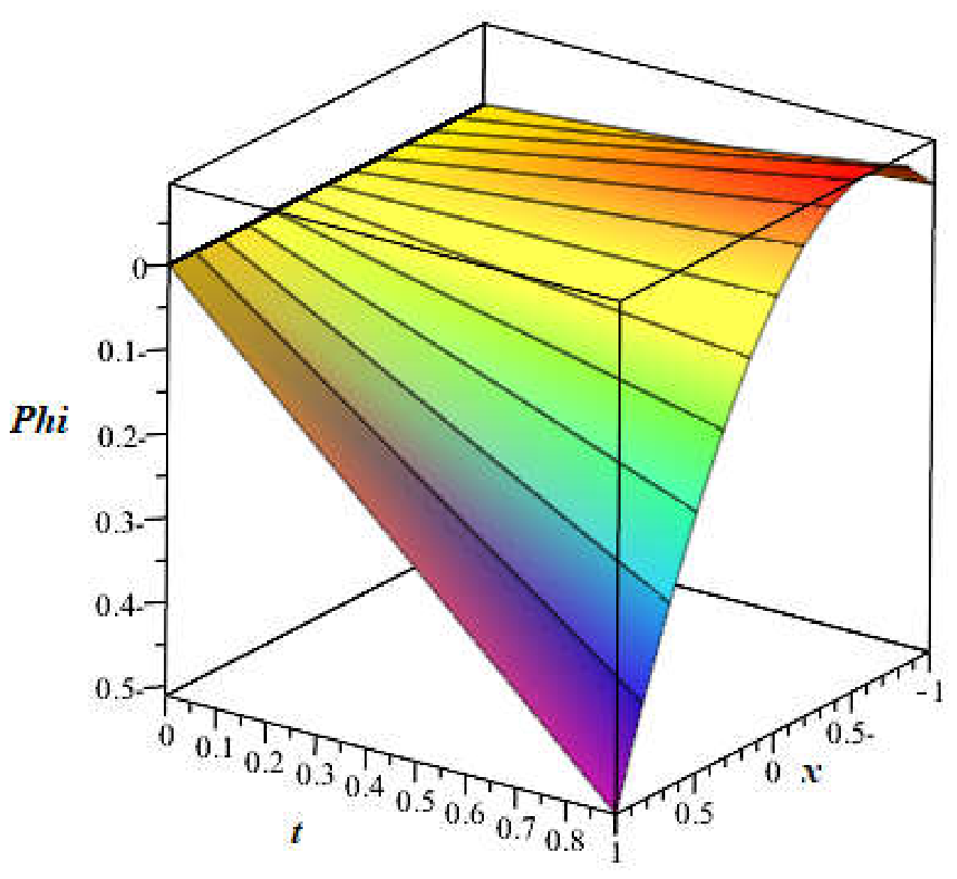
Figure 2.
Nonlocal w =
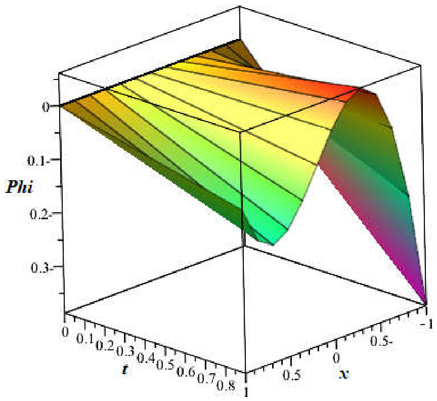
Figure 3.
Nonlocal
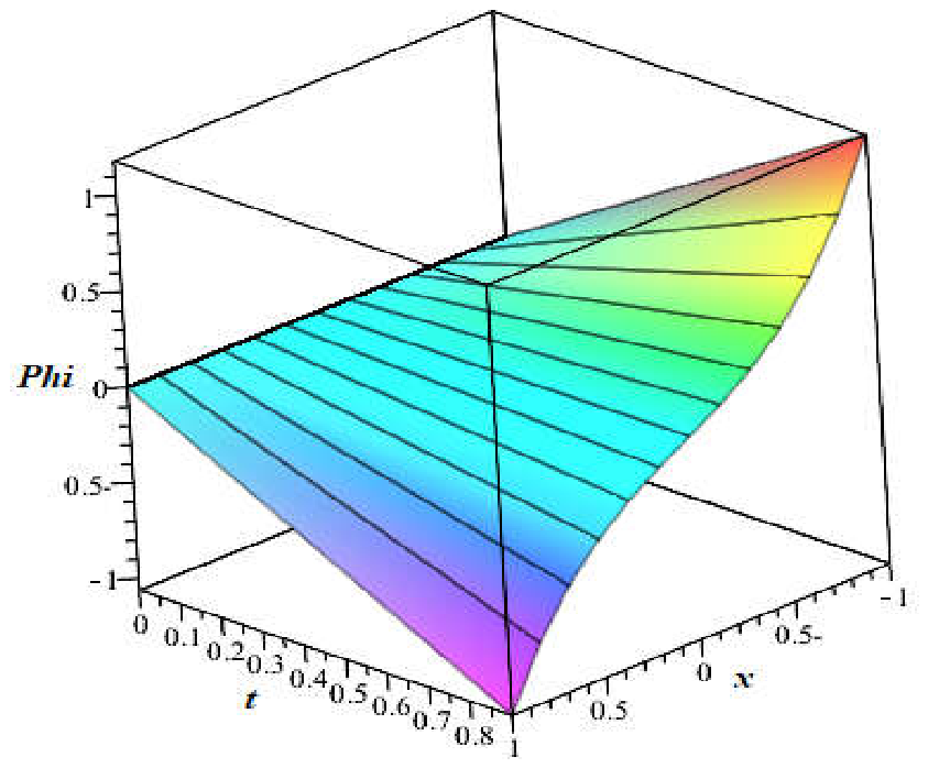
Figure 4.
Nonlocal
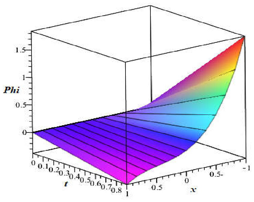
Figure 5.
Local
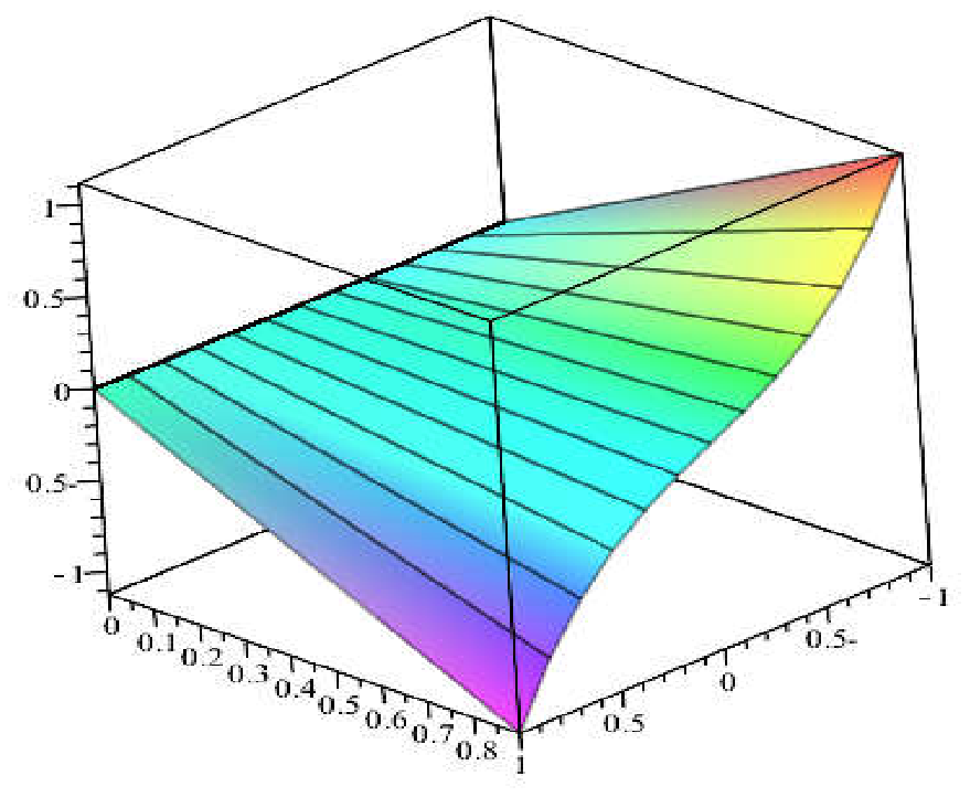
Figure 6.
T=0.55 N=8 Nonlocal
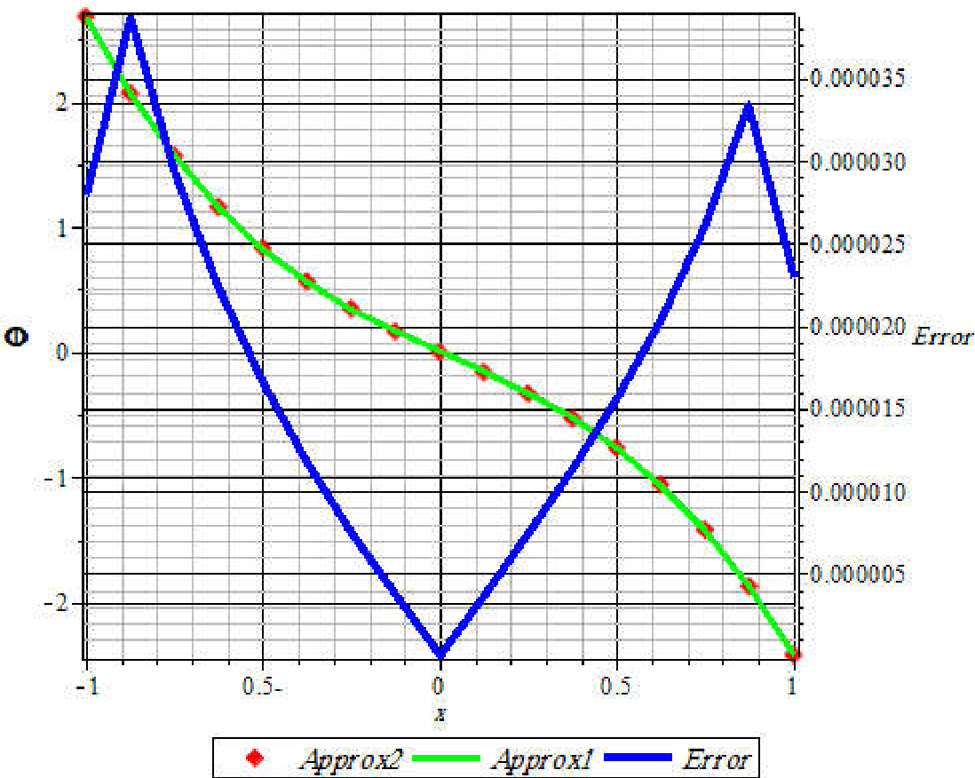
Figure 7.
Figure 7. T=0.55, N=8 Nonlocal
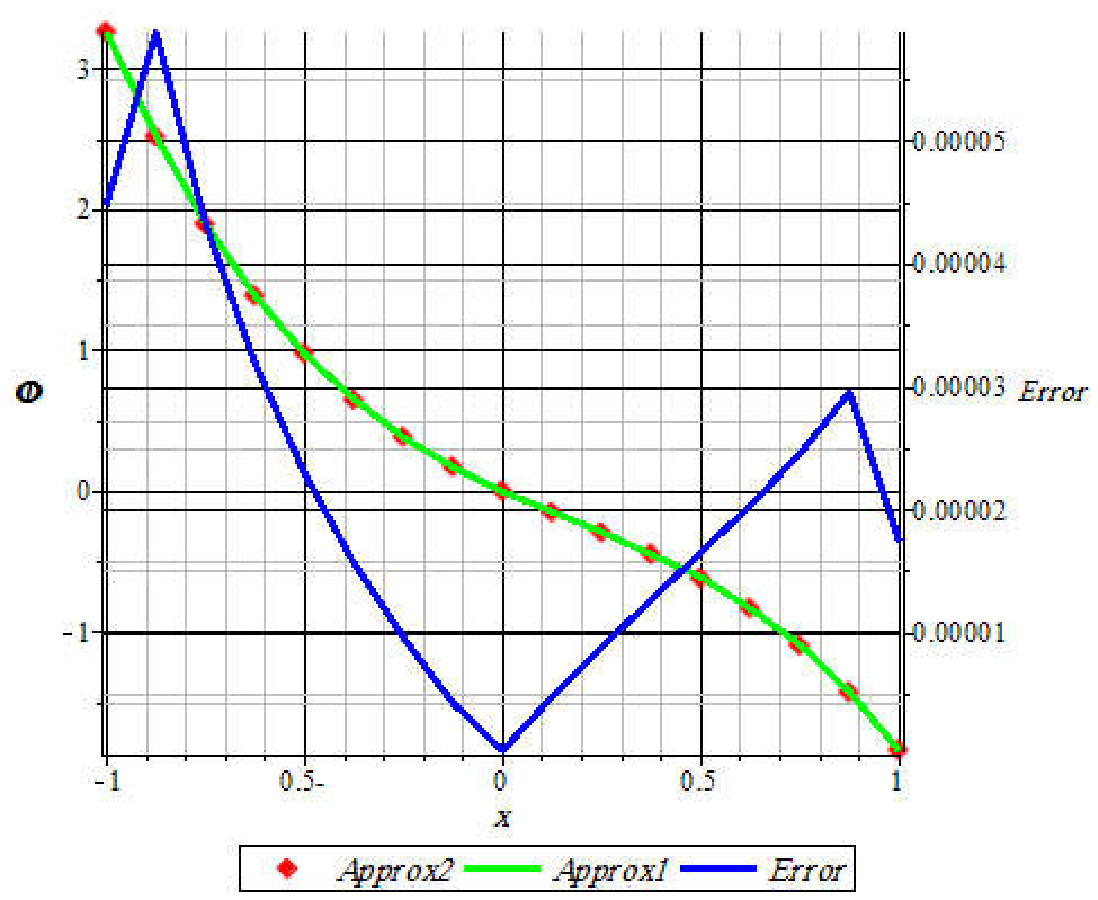
Table 1.
Convergence rate in local conditions with time
| Max. Error | Rate | ||
| 0.02 | 3 | 8.5×10⁻⁶ | 1.16 |
| 6 | 3.8×10⁻⁶ | 2.21 | |
| 12 | 8.2×10⁻⁷ | --- | |
| 0.45 | 3 | 1.3×10⁻⁴ | 4.2 |
| 6 | 7.1×10⁻⁶ | 3.77 | |
| 12 | 5.2×10⁻⁷ | --- |
Table 2.
Convergence rate in local conditions with time
| Max. Error | Rate | ||
| 0.02 | 3 | 1.2×10⁻³ | 1.07 |
| 6 | 5.7×10⁻⁴ | 1.08 | |
| 12 | 2.7×10⁻⁴ | --- | |
| 0.45 | 3 | 1.9×10⁻³ | 0.79 |
| 6 | 1.1×10⁻³ | 0.72 | |
| 12 | 6.7×10⁻⁴ | --- |
Table 3.
Convergence rate in local conditions with time
| Max. Error | Rate | ||
| 0.02 | 3 | 4.1×10⁻³ | 1.19 |
| 6 | 1.8×10⁻³ | 1.03 | |
| 12 | 8.8×10⁻⁴ | --- | |
| 0.45 | 3 | 5.9×10⁻³ | 0.98 |
| 6 | 3.0×10⁻³ | 0.51 | |
| 12 | 2.1×10⁻³ | --- |
Table 4.
Convergence rate in nonlocal conditions with time .
| Max. Error | Rate | ||
| 0.02 | 3 | 6.8×10⁻⁶ | 1.18 |
| 6 | 3.0×10⁻⁶ | 2.3 | |
| 12 | 6.0×10⁻⁷ | --- | |
| 0.45 | 3 | 1.0×10⁻⁴ | 4.03 |
| 6 | 6.1×10⁻⁶ | 3.86 | |
| 12 | 4.2×10⁻⁷ | --- |
Table 5.
Convergence rate in nonlocal conditions with time .
| Max. Error | Rate | ||
| 0.02 | 3 | 1.0×10⁻³ | 1.15 |
| 6 | 4.5×10⁻⁴ | 1.32 | |
| 12 | 1.8×10⁻⁴ | --- | |
| 0.45 | 3 | 1.5×10⁻³ | 0.79 |
| 6 | 8.7×10⁻⁴ | 0.78 | |
| 12 | 5.0×10⁻⁴ | --- |
Table 6.
Convergence rate in nonlocal conditions with time .
| Max. Error | Rate | ||
| 0.02 | 3 | 3.2×10⁻³ | 1.00 |
| 6 | 1.6×10⁻³ | 1.15 | |
| 12 | 7.2×10⁻⁴ | --- | |
| 0.45 | 3 | 4.8×10⁻³ | 0.83 |
| 6 | 2.7×10⁻³ | 0.67 | |
| 12 | 1.7×10⁻³ | --- |
Table 7.
Convergence rate in nonlocal conditions of logarithmic kernel with time .
| N | Max. Error | Rate |
| 3 | 1.3×10⁻¹¹ | 5.01 |
| 6 | 4.2 ×10⁻¹² | 1.10 |
| 12 | 9×10⁻¹² | --- |
Table 8.
Convergence rate in nonlocal conditions of logarithmic kernel with time .
| N | Max. Error | Rate |
| 3 | 8.5×10⁻⁵ | 0.77 |
| 6 | 5.0 ×10⁻⁵ | 0.84 |
| 12 | 2.8×10⁻⁵ | --- |
Table 9.
Convergence rate in nonlocal conditions of logarithmic kernel with time .
| N | Max. Error | Rate |
| 3 | 9.1×10⁻³ | 0.73 |
| 6 | 5.5 ×10⁻³ | 0.65 |
| 12 | 3.5×10⁻³ | --- |
Disclaimer/Publisher’s Note: The statements, opinions and data contained in all publications are solely those of the individual author(s) and contributor(s) and not of MDPI and/or the editor(s). MDPI and/or the editor(s) disclaim responsibility for any injury to people or property resulting from any ideas, methods, instructions or products referred to in the content. |
© 2026 by the authors. Licensee MDPI, Basel, Switzerland. This article is an open access article distributed under the terms and conditions of the Creative Commons Attribution (CC BY) license (http://creativecommons.org/licenses/by/4.0/).
Copyright: This open access article is published under a Creative Commons CC BY 4.0 license, which permit the free download, distribution, and reuse, provided that the author and preprint are cited in any reuse.


