

Submitted:
30 June 2026
Posted:
01 July 2026
You are already at the latest version
Abstract
This paper surveys recent results and methods in the study of permutation polynomials and their compositional inverses over finite fields. In particular, we focus on the recently developed local method and emphasize how it provides a unified and reinterpretative framework for the compositional inverses of permutation polynomials previously obtained by various other techniques (such as piecewise methods, linearized polynomials, decomposition method, the original commutative diagram method). By revisiting these classical results, we reveal the deeper advantages of the local method in understanding the structure of permutation polynomials and the explicit expressions of their inverses. This survey aims to give readers a systematic and profound understanding of the principles, applicability, and intrinsic connections of the local method to existing approaches.
Keywords:
finite field
; polynomial
; permutation polynomial
; local criterion
1. Introduction
Let be the finite field with q elements and denote the multiplicative group with the nonzero element in , where q is a prime power. Let be the ring of polynomials in a single indeterminate x over . A polynomial is called a permutation polynomial (PP) of if its associated polynomial mapping from to itself is bijective. The unique polynomial denoted by over such that is called the compositional inverse of Furthermore, is called an involution when
The study of permutation polynomials and their compositional inverses over finite fields in terms of their coefficients is a classical and difficult subject which attracts people’s interest partially due to their wide applications in coding theory [1,2,3], cryptography [4,5], combinatorial design theory [6], and other areas of mathematics and engineering [7,8].
In general, determining whether a polynomial over a finite field is a permutation polynomial is challenging. Moreover, computing the coefficients of the compositional inverse of a permutation polynomial is even more difficult, except for several well-studied classes such as monomials, linearized polynomials, and Dickson polynomials, which prossess a well-defined structure. Q. Wang [9] has summarized the current methods used in the study of the compositional inverses of permutation polynomials, including the experimental method, the power sum method, the matrix method, the group algebra method, the piecewise method, the decomposition method, the commutative diagram method, and the local method. On the basis of the existing classification system, this paper further supplements and refines the theoretical system of permutation polynomials via targeted in-depth discussions. Specifically, this survey consists of two core parts. It first conducts an in-depth exploration of the AGW criterion and local criterion, and systematically sorts out the algebraic structure-based theoretical methods for permutation polynomial construction. Furthermore, different from the macroscopic classification in previous studies, this paper focuses on the local method, rederiving and reinterpretating all existing formulas for compositional inverses of permutation polynomials. This work standardizes the relevant theoretical derivation logic and complements the existing research system, offering a solid and systematic theoretical basis for subsequent related studies and practical applications.
2. Methods on Permutation Polynomials over Finite Fields
2.1. AGW Criterion, Local Criterion and Local Method
Before discussing the compositional inverse of permutation polynomials, this section first introduces several fundamental theorems for constructing permutation polynomials, laying the groundwork for subsequent analysis.
2.1.1. The AGW Criterion: Theory and Further Understanding
The Akbary–Ghioca–Wang (AGW) criterion [10] [Lemma 1.1] is an important method for constructing PPs. By providing necessary and sufficient conditions for a polynomial to be a permutation via a commutative diagram, this criterion not only unifies many classical constructions of permutation polynomials, but also yields a large number of new ones, thereby significantly advancing the study of permutation polynomials.
Theorem 1.
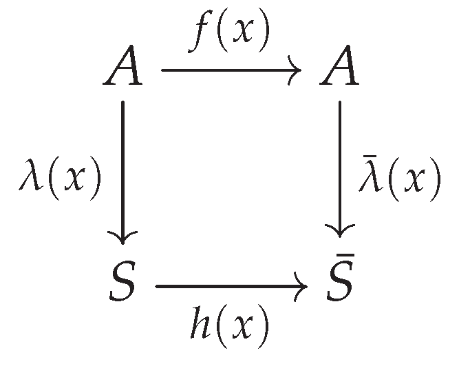
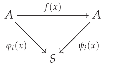
[10] [AGW criterion] Let and be finite sets with , and let , , and be maps such that If both and are surjective, then the following statements are equivalent:
(i) is bijective (a permutation of A); and
(ii) is bijective from S to and is injective on for each
Figure 1.
The AGW criterion
Building on the AGW criterion recalled above, we next present several related characterizations established in [11].
Theorem 2.
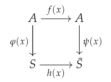
[11] [Theorem 2.3] Let A and S be finite sets, a map, and be a surjective map. Then f is a bijection if and only if the following conditions hold:
(i) f is injective on each for all ;
(ii) for each bijection , there exists a uniquely determined surjective map such that the following diagram commutes:
As a straightforward generalization of Theorem 2, Yuan [11] obtained the following result:
Theorem 3.
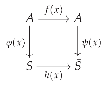
[11] [Theorem 2.4] Let A and S be finite sets and let be a map and be a surjective map. Then is a bijection if and only if the following conditions hold:
(i) is injective on each for all ;
(ii) for each bijection , where is a set with , there exists an uniquely determined surjective map such that the following diagram commutes
Theorem 3 shows that every permutation polynomial can be characterized by the AGW criterion.
Further equivalent characterizations for bijective self-maps on finite sets are also provided in the same reference, as listed below.
Theorem 4.
[11] [Lemma 2.5] Let be finite sets, a map and a surjective map. Then f is a bijection if and only if
(i) is injective on each for all .
(ii) If , then .
Moreover (ii) is equivalent to for any distinct .
Theorem 5.
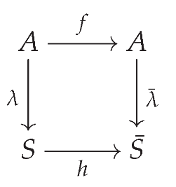
[11] [Lemma 2.5] Let and be finite sets with , a map and a surjective map. Then is a bijection if and only if the following two conditions hold:
(i) is injective on each for all .
(ii) There exists a pair of maps such that is a surjective, is a bijective and the following diagram commutes.
The following theorem gives a unique surjection characterization together with an enumeration formula for such bijections.
Theorem 6.
[11] [Theorem 2.8] Let A and S be finite sets. Assume that and are maps. If is surjective and is injective on for each then is bijective if and only if there exists a unique surjection such that Moreover, there are bijections determined by the map
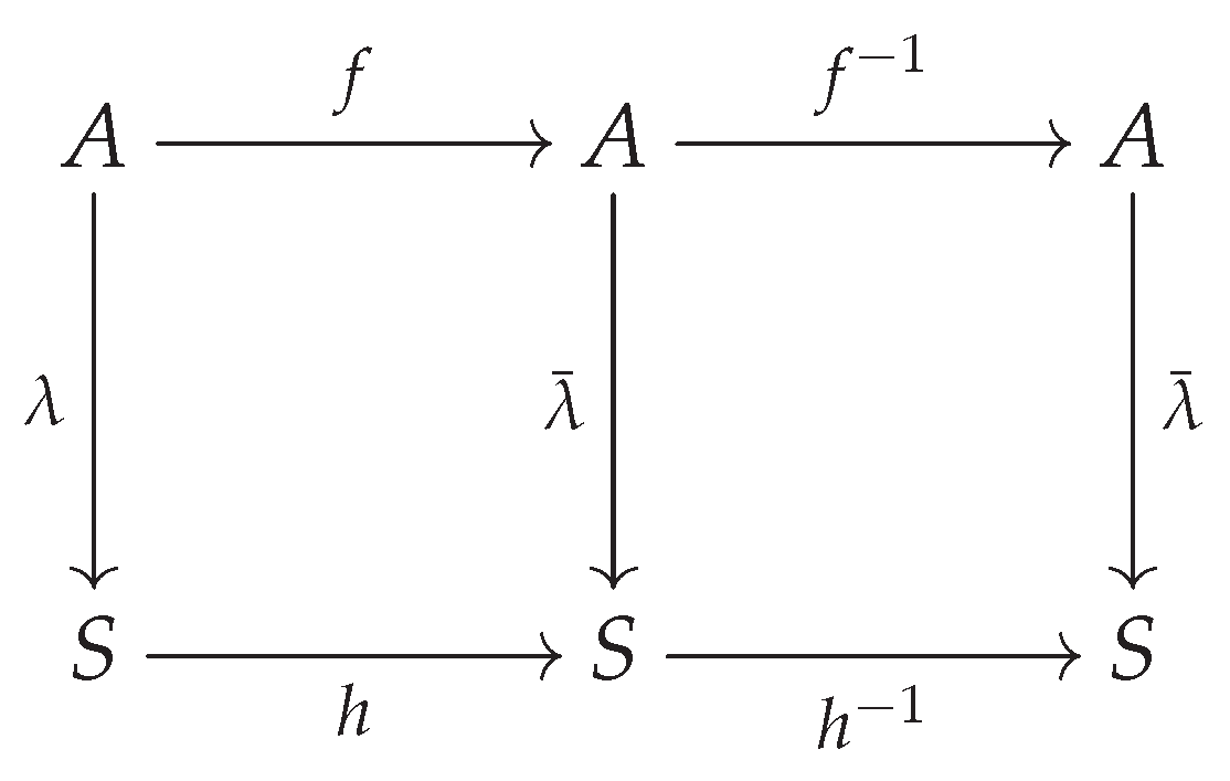
The dual diagram of the AGW criterion was put forward by Yuan in [12]. This dual theoretical framework acts as an important tool to derive compositional inverses of PPs when applying Theorem 14 (See Theorems 27, 33 for more details).
Theorem 7.
[12] [Theorem 2.6] Let the notations be defined as in Lemma 1. If is a bijection, and are the compositional inverses of and respectively, then we have
i.e., the following diagram commutes
Figure 2.
The dual diagram of AGW criterion
2.1.2. The Group Structure of the Set of Permutation Polynomials: A Perspective Based on the AGW Criterion
In 1991, Wan and Lidl [13] showed that all permutation polynomials of the form from a group under composition and this group is isomorphic to a generalized wreath product. Yuan [12,14] obtained a similar result for other permutation polynomials over finite fields and determine their group structure.
Theorem 8.
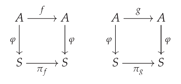
[12] [Theorem 4.1] Let be finite sets and let be a surjective map. Let be the set of all bijections such that , where is a bijection. Then forms a group under composition.
The following two commutative diagrams hold:
Theorem 9.
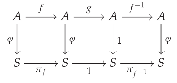
[12] [Theorem 4.2] Let the notations be as in Theorem 8, and let , where denotes the identity map on S. Then is a normal subgroup of .
The following two commutative diagrams holds:
Subsequently, Yuan [14] gave the following conclusion for the case where A is a group and is an epimorphism in Theorem8. We first introduce the relevant notation.
The following definitions can be found in [15] [Chapter 7]. Let K be a subgroup (not necessarily normal) of a group G. Then a subgroup is a complement of K in G if and , where .
Definition 1.
A group G is a semidirect product of K by Q, which is denoted by , if and K has a complement . One also says that G splits over K.
Definition 2.
Let D and Q be groups, Ω be a finite Q-set, and , where for all . Then the wreath product of D by Q, denoted by , is the semidirect product of K by Q, where Q acts on K by for and . The normal subgroup K of is called the base of the wreath product.
When the group D is finite, we have ; if Q is also finite, then
Theorem 10.
[14] [Theorem 3.1] Let A be a finite group of order n. Let be a subgroup with and be an epimorphism. Let be the set of all bijections such that , where is a bijection. Then and .
2.1.3. The Local Criterion
Next, we will introduce the Local Criterion. Although the Local Criterion is equivalent to the AGW criterion, it provides a more transparent formulation for our purposes: it reveals the fundamental mechanism of constructing permutation polynomials via map compositions (See Theorem 27, Remark 2, Theorem 33 and Remark 4 for further assistance). We state the criterion as follows.
Theorem 11.
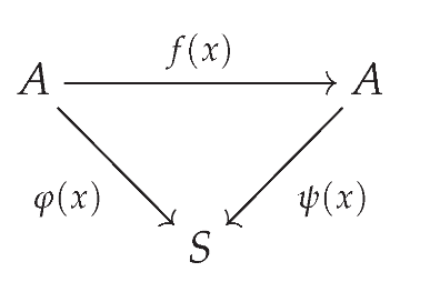
[16] [Lemma 2.1 ](Local Criterion) Let A and S be finite sets, and let be a map. Then is a bijection if and only if for any surjection the composition is a surjection, and is injective on for each
Corollary 1.
Let A and S be finite sets, and let be a surjective map. If the map is bijective, then is injective on for each
From the local criterion, determining whether is a permutation polynomial requires the following two conditions:
(1) is a surjection from A to S;
(2) For each , the restriction of to is injective.
This naturally raises the following question: if only one of the above conditions is satisfied, but we appropriately increase the number of maps satisfying that condition, can we still conclude that is a permutation polynomial from A to A? Specifically:
(i) Generalization of the surjectivity condition: Let (), and let be surjective. Suppose that for each i, the composition is a surjection from A to . Does it follow that f is a permutation from A to A?
(ii) Generalization of the injectivity condition: Let , and let be surjective. Suppose that for each i and each , the restriction is injective. Does it follow that f is a permutation from A to A?
The above two problems lead respectively to the central concepts in this subsection — surjective systems and injective systems.
1. surjective systems
We introduce surjective systems at first.
Definition 3.
[17] For a prime power let be a polynomial over . Assume that are nonempty finite sets of with and are surjections from to If is a permutation polynomial over if and only if are surjective from to , then the polynomial is called the local permutation polynomial over with respect to
Theorem 12.
[17] Let A and be finite sets, and let be surjective maps and be a map. Suppose that is a permutation polynomial if and only if are surjective from A to . Then for any permutation polynomial is a permutation polynomial if and only if for are surjections from A to
2. injective systems
We recall several definitions and results concerning injective systems for permutation polynomials, which were recently proposed and systematically investigated in [11].
Definition 4.
Let q be a prime power, S a proper non-empty subset of , and let be a surjective map. We say that is injective for if is injective for any . Let for . We say that is injective for if is injective for each .
For further understanding the notation of is injective for , the following result was established in [11]. .
Lemma 1.
Let q be a prime power and d be a positive integer with . Then is injective for if and only if .
As a direct consequence of Lemma 1, the following corollary holds.
Corollary 2.
Let q be a prime power. Then is injective for if and only if , i.e., is a PP over .
The general equivalence between the permutation property and injectivity with respect to polynomial families was presented in [11] as follows.
Proposition 1.
[11] Let q be a prime power, and let for . Suppose that is a PP if and only if is injective for . Then for any two distinct elements , there exists some such that .
Conversely, if for any two distinct elements , there exists some such that . Then is a PP if and only if is injective for .
Based on the above equivalent characterization, the formal definition of injective systems for permutation polynomials was introduced in [11].
Definition 5.
[11] Let q be a prime power, and for , let be non-constant polynomials in . We say that is an injective system for PP over provided that is a PP if and only if is injective for .
Furthermore, a concrete family of injective systems via trace polynomials was also provided in [11].
Proposition 2.
Let q be a prime power and let be a positive integer. Then is an injective system for PP over .
Motivated by the above results, we propose the following notation.
Definition 6.
[11] Let q be a prime power, S a proper non-empty subset of , and let be a surjective map. We say that is injective for if is injective for any . Let for . We say that is injective for if is injective for each .
First, a lower bound on the number of polynomials contained in any injective system is given as follows.
Proposition 3.
Let be a prime power and for be non-constant maps. If is an injective system for PPs over , then .
Second, an explicit infinite family of injective systems constructed via trace polynomials over extension fields is characterized below.
Proposition 4.
Let q be a prime power and let be a positive integer. Then
is an injective system for PPs over .
Furthermore, Yuan proved that we may drastically shrink the above trace family while still preserving the injective system property, as summarized in the following existence theorem.
Theorem 13.
Let q be a prime power and let be a positive integer. There exists a set such that is an injective system for .
2.1.4. The Local Method
Based on the local criterion, Yuan [16] established a local method that can determine whether a polynomial is a permutation polynomial while simultaneously deriving its compositional inverse.
The local method is a powerful and effective tool for constructing permutation polynomials over finite fields and computing their compositional inverses. Originating from number theory and algebraic theory, this method adopts the local–global principle to characterize polynomials over finite fields. Specifically, it deduces the global permutation property of a polynomial from its local characteristics on subsets of the finite field. The essence of the local method lies in characterizing the inherent functional relationship between the polynomial and the variable x, which is achieved by analyzing the composite mappings for a family of properly chosen mappings .
Theorem 14.
[16] [Theorem 2.2] (Local method) Let q be a prime power and be a polynomial over Then is a permutation polynomial over if and only if there exist nonempty finite subsets , of and maps , such that and where Moreover, the compositional inverse of is given by
The essence of the local method lies in examining the composition (for several polynomials ) to determine its functional relationship with
2.2. Algebraic Structure of Permutation Polynomials
It is well known that and are isomorphic as vector spaces over . This isomorphism allows us to study permutation polynomials by translating a univariate polynomial into a multivariate polynomial map .
Based on the basic properties of the trace, we recall the following criterion for -space homomorphisms.
Lemma 2.
[18] [Lemma 4.2] Let be a map from to . Then is an -space homomorphism if and only if for some .
Based on the trace representation above, the full characterization of -vector space homomorphisms from to is given in the same reference.
Theorem 15.
[18] Let be an -vector space homomorphism, then there are n elements such that
Moreover, ρ is an -vector space isomorphism if and only if is a basis of over , and when this occurs, its compositional inverse is given by:
where is the ordered dual basis of .
Symmetrically, homomorphisms in the reverse direction admit a dual description, as recorded below.
Theorem 16.
[18] Let be an -vector space homomorphism, then there exist n elements such that
Moreover, η is an -vector space isomorphism if and only if is a basis of over , and when this occurs, its compositional inverse is given by:
where is the ordered dual basis of .
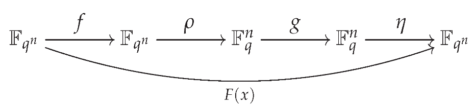
Combining the isomorphisms and characterized above with an arbitrary permutation g on , Yuan derived the following compositional criterion for permutation polynomials over .
Theorem 17.
[18] [Theorem 1.1] Given a PP . Let , be -vector space homomorphisms, and let g be a map from to . Then for any and , we have
Moreover, is a PP of if and only if the following two conditions hold:
(i) Both and are bases of over ;
(ii) permutes .
Further, we take into account the two fundamental polynomial rings, namely and , defined over the finite field , and a profound algebraic property is then exhibited as follows. For simplicity, let denote the set of all mappings from A to B.
Theorem 18.
[18] Let and be -vector spaces, equipped with addition and scalar multiplication operations. Then ψ given by
We now shift our attention to equivalence relations for multivariate permutation polynomial systems over , which were first introduced in [19].
Definition 7.
[19] [Definition 3.1] Let q be a prime power and n be a positive integer. Two polynomial systems and , with , are called linearly equivalent if there exist nonsingular linear transformations and such that .
From this definition, it immediately follows that F is a permutation of if and only if G is a permutation of . On the other hand, observe that the identity map is trivially a permutation system over . Moreover, modifying the i component of such polynomial system by adding terms that depend solely on previously determined variables preserves its permutation properties. This motivates the following notion of coordinate shift equivalence:
Definition 8.
[19] [Definition 3.2] Let q be a prime power and n be a positive integer. Given two polynomial systems defined as:
where and each . We say F and G are coordinate shift equivalent (abbreviated as CS equivalent). In the special case when , the systems reduce to: and .
Their investigation commences with quadratic polynomial systems. Let denote the equivalence of two polynomial systems F and G under the combined operations of linear equivalences and CS equivalences. They provide complete characterizations of bivariate quadratic permutations over finite fields.
Theorem 19.
[19] [Theorem 3.1] Let be a finite field of characteristic p. A quadratic polynomial system defined by
is a permutation over if and only if:
(i) for odd p, ,
(ii) for even p, , , , or with being a linearized permutation over .
Use the same method, they provide complete characterizations bivariate 3-homogeneous permutations over finite fields.
Theorem 20.
[19] [Theorem 3.2] Let be a finite field with . The system of 3-homogeneous polynomials defined by
where , and , is a permutation of if and only if both and are irreducible over , and one of the following occurs:
(i) for some constant .
(ii) , and the rational function is equivalent to (for ) or (for ), where are degree-one rational functions in and is either 0 or a quadratic nonresidue.
They determine all binomial permutations of the form over a finite field with , as an application of Theorem 20 and obtain the following result.
Proposition 5.
[19] [Propsotion 3.10] Let q be an odd prime power with characteristic , and let with . Then permutes if and only if one of the following holds:
(1) If , then
(1.1) and ;
(1.2) and or ;
(1.3) and .
(2) If , let be a quadratic nonresidue, and take where . Writing with . Then either:
(2.1) , (where σ satisfies ) and the equation has no roots in ; or
(2.2) and , for some arbitrary .
3. Methods on the Inverse of Permutation Polynomial over Finite Fields
In this section, permutation polynomials are classified according to their algebraic forms. It should be noted that this classification is not strictly exclusive; for instance, is both a linearized polynomial and a polynomial of the form . The classification thus reflects the different methods historically used to study permutation polynomials, rather than a purely set-theoretic categorisation. For each class, we first present a review of the research history concerning its compositional inverse, and then compute its compositional inverse via the local method.
3.1. Inverses of Monomials
For positive integer is a PP of if and only if All invertible monomials form a group of order under the operation of composition, where is Euler’s totient function. The inverse of over is where The case of monomials being trivial, we forego the derivation of its compositional inverse using the local method.
3.2. Inverses of Dickson PPs
The Dickson polynomial of the first kind of degree n with parameter is given as
where denotes the largest integer
A fundamental property of is that for any ,
The following result, established by Li et al. [21], provides the compositional inverse of a Dickson polynomial under the permutation condition. For the convenience of the reader, we retain the proof.
Theorem 21.
[21] [Lemma 4.8] Let q be a prime power and . Let m be a positive integer satisfying . Then the compositional inverse of the Dickson polynomial over is
Proof.
Let and such that . Then for any ,
Therefore, the compositional inverse of the Dickson polynomial over is . □
Remark 1.
From the proof of Theorem 21, we may take , which yields . Hence, by Theorem 14, we obtain . This is essentially the proof itself, which does not yet reveal the advantage of the local method.
The polynomial over , where and , is actually the Dickson PP (see [22]), and its inverse on is by Theorem 21, where .
The polynomial over with and is indeed the Dickson polynomial (see [23]), and its inverse is by Theorem 21.
3.3. Inverses of Linearized PPs
Linearized polynomials are always taken as
We denote by the set of all linearied polynomials in the form (5). Equipped with the composition of polynomials in , forms non-commutative -algebra. Wu and Liu [24] characterize the algebra , that is
where is the dual space of over , is the so-called composition algebra on , and is an algebra formed by all matrices over of the form
which are called Dickson matrices. It is clear that the set of all non-singular Dickson matrices form a group.
Based on the result from (6), the following identity holds:
Hence, Wu and Liu [24] were able to derive the compositional inverse of a linearized permutation polynomial over Unlike their approach, which relies on various properties of linearized polynomials as theoretical groundwork, we adopt the Local method [17] to directly obtain the compositional inverse without the aforementioned preparation. For the convenience of the reader, a detailed proof using the Local method is provided below.
Theorem 22.
[24] [Theorem 4.5][17] Let be a linearized permutation polynomial and be its associated Dickson matrix. Then
where is the th cofactor of , and the determinant of is
Proof.
For , set and . Since the associated Dickson matrix is non-singular and
multiplying both sides on the left by yields
Recalling that , where is the adjugate matrix of , we obtain
Taking the first row of this matrix identity gives the scalar equation
where are the entries from the first row of . Finally, by Theorem 14, the compositional inverse of is given by
□
The general theorem above provides a theoretical approach for obtaining the compositional inverse of a linearized permutation polynomial via the determinant and the th cofactor of its associated Dickson matrix. Below, we give three examples of linearized polynomials whose compositional inverses are obtained through their Dickson matrices.
Example 3.3.1. Coulter and Henderson characterized the following linearized permutation binomial in [25]:
and Wu subsequently determined its compositional inverse in [26] via the determinant and the -th cofactor of its associated Dickson matrix.
Inspired by the idea in Section 9 of Wang [9], which presents a new and simpler proof for the compositional inverse of such a binomial, we reformulate Wang’s proof using the language of the local method.
Theorem 23.
Proof.
Let In this case, for , we choose and
Obviously,
Hence, it follows from Theorem 14 that f is a PP if and only if , and the compositional inverse of f is
This completes the proof. □
We summarize in Table the results on permutation polynomials of the form with degree less than 7, obtained based on Theorem 23.

Table 1.
Linearized permutation binomials of the form and their inverses
| Polynomial | Inverse | Conditions |
|---|---|---|
| , a not a square | ||
| , a not a square | ||
| , | ||
| , a not a fourth power | ||
| , a not a sixth power |
Example 3.3.2. Wu [26] studied the linearized polynomial by using recurrences to compute the determinant of its Dickson matrix and the -cofactors. Based on this, he gave a criterion for to be a permutation polynomial over and an explicit formula for its inverse (see [26] [Theorem 3.2.29]).
Taking , the polynomial reduces to over . To state the result of Zheng et al. [22] for this special case, we need the following recurrence sequence:
where .
Theorem 24
(Corollary 4, [22]). Let , where and . Then is a permutation polynomial over if and only if . Moreover, if permutes , its inverse is given by
Example 3.3.3. Using heavy computation of determinants, Wu [27] obtained the following result.
Theorem 25.
[27] [Theorem 2.2] Let n be an odd positive integer, and let such that Then
is a permutation polynomial over with compositional inverse
where the coefficients for are given by
Tuxanidy and Wang [28] generalized Theorem 25 to the general q-case by decomposition method.
Regarding the compositional inverse of linearized polynomials, there is another result as follows.
Bastos [29] studied the inverses of linearized permutation polynomials over with coefficients in , under the condition that .
The key observation is that, for such a linearized polynomial, its q-associate polynomial is coprime to . Consequently, the conventional associate polynomial of its compositional inverse can be computed via the extended Euclidean algorithm. Let . The primitive idempotents in are easily described using the -algebra isomorphism between and the group algebra of a cyclic group C of order n. By exploiting the decomposition of via these idempotents, Bastos derived explicit formulas for the inverses.
Theorem 26.
[29] [Theorem 26] Let be the set of primitive idempotents of Given a linearized permutation over and its conventional q-associate, then can be written as
in which for Furthermore, the conventional associate of the compositional inverse of is given as
This result theoretically provides a method for constructing the inverse permutation of specific linearized polynomials over . However, as the method relies on a special coefficient structure, it lacks general applicability for computing the inverse of arbitrary linearized permutation polynomials. Therefore, it is only briefly mentioned in this paper without an in-depth discussion.
3.4. Inverses of Permutation Polynomials of the Form
For permutation polynomials of the form , the inductive construction involves compositional inverses of two related families: those of the form and those of the form . In the Local method (Theorem 14), the associated functions are chosen differently for these two families. Accordingly, the two cases are treated separately below.
3.4.1. Permutation Polynomials of the Form
A result for polynomials of the form to be permutations was given by Akbary et al. [10] by AGW criterion.
Lemma 3.
[10] [Theorem 6.3] For a prime power q and a positive integer n, let S be a subset of containing Assume that be any polynomials such that and Let be a polynomial satisfying
(1) and
(ii) for all and all
Then the polynomial is a permutation polynomial over if and only if induces a permutation over
The commutative diagram for the above permutation polynomial is as follows.
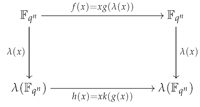
Using the commutative diagram method (see [9,30] for details), Niu et al. [30] derived an explicit expression for the compositional inverse of the permutation polynomial described in Lemma 3. In what follows, we provide an alternative proof of their result by employing the local method (Theorem 14). This approach not only simplifies the original argument but also yields the following result.
Theorem 27.
[30] [Theorem 22 ] Let the notations be defined as in Lemma 3. Let be a permutation polynomial over and be the compositional inverse of over Then the compositional inverse of over is
Proof.
By assumption, we have Then by Lemma 7, we obtain
Let and Note that
by It follows from Lemma 14 that the compositional inverse of is
We are done. □
Remark 2.
Theorem 27 (namely Theorem 22 in [30]) and Lemma 3 can be revisited from the perspective of the local method. We present two remarks below: one simplifies the expression form of Theorem 27, and the other discusses the conditional constraints of Lemma 3 as well as the intrinsic role of the local criterion.
(1) Simplification of the expression. The compositional inverse given in Theorem 27 is
However, this expression is not in its simplest form. Indeed, since , we have
so the numerator simplifies to x. Consequently,
(2) On the conditions of Lemma 3 and the role of the local criterion. The two conditions in Lemma 3 (namely and for all , ) are rather restrictive. Their purpose is to construct a polynomial such that the commutation relation holds.
The local criterion is the essential core for determining permutation polynomials: it reveals how to establish a connection between variables through functional composition, thereby determining whether a given polynomial is a permutation polynomial. From this criterion, the local method (Theorem 7) is derived, which proceeds by finding suitable functions and satisfying , thereby establishing a direct relationship between and the variable x, and using this relationship to determine whether f is a permutation polynomial.
Within this framework, the commutation relation can be rewritten as , which is precisely a concrete instance of . The AGW criterion employed in Lemma 3 serves to provide a specific constructive way of finding such and (here, λ and ) for the local method. However, the strong additional conditions in that lemma are not required by the local criterion or the local method themselves; they are merely one particular construction that realizes the desired relation. In other words, the local criterion reveals the core mechanism of constructing mappings via functional composition; the local method realizes this mechanism by constructing mappings and satisfying , while the AGW criterion in Lemma 3 serves as an auxiliary constructive tool.
In light of the above discussion — namely that the local criterion, not the restrictive AGW conditions, is the essential core — we generalize Lemma 3 to a more general form using the local criterion and method. The proof is analogous to that of Theorem 27, and is therefore omitted.
Theorem 28.
For a prime power let
where and be polynomials over such that for all If there exists a polynomial such that then the polynomial is a permutation polynomial over if and only if is injective on for each
Moreover, if and permute , let be the compositional inverse of over Then the compositional inverse of is given by
Remark 3.
It should be noted that the conclusion of Theorem 28 is derived from the Local Criterion applied to polynomials of the form . Meanwhile, Theorem 3.3 in [12] obtains exactly the same characterization based on the AGW Criterion.
3.4.2. Permutation Polynomials of the Form
The study of permutation polynomials of the form was initiated by Wan et al. [13]. Subsequently, independent results on this family were obtained by Park et al. [31], Wang [32], and Zieve [33]. A unifying result from these works is the following lemma, which provides a useful criterion (or description) for such polynomials to be permutations.
Lemma 4.
[31] [Theorem 2.3][13] [Theorem 1. 2][32] [Theorem 1][33] [Lemma 2.1] Let q be a prime power and , where and l is an integer. Then permutes if and only if
(i) and
(ii) permutes
The commutative diagram for the above permutation polynomial is as follows.
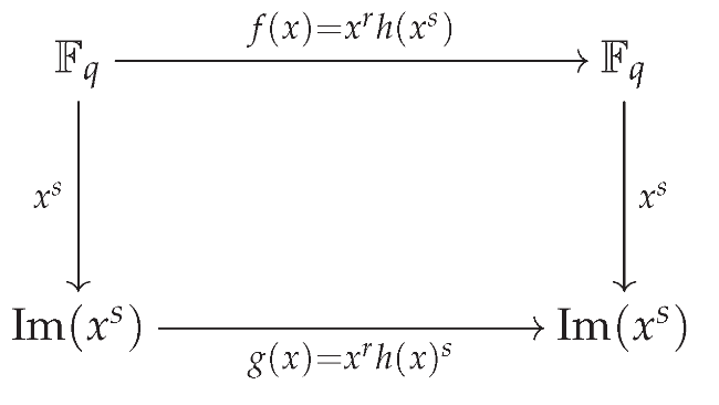
Niu et al. [30] [Theorem11] determined the compositional inverse of the permutation polynomial in Lemma 4 using the commutative diagram method. Yuan [16] revisited this theorem and provided a new proof via the local method. For the convenience of the reader, we present Yuan’s proof in full detail below.
Theorem 29.
Proof. 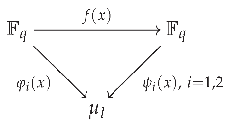
By the assumptions, we have the following commutative diagrams
where
We have
It follows from Theorem 14 that
This completes the proof. □
Assume that the notations are as defined in Theorem 29. According to this theorem, the computation of the compositional inverse of a permutation polynomial of the form reduces to determining the inverse map of the polynomial on the set .
As a concrete illustration, consider the family . Zheng et al. [23] explicitly computed for , and consequently obtained the compositional inverse of .
Theorem 30.
[23] [Theorem 3.4] Let where , and Let
If is a PP over then its inverse on is where
When , they obtain
Theorem 31.
[23] [Theorem 5.2] Let where , q is odd and Let
(i) If is even, then is a PP of if and only if In this case,
(ii) If is odd, then is a PP of if and only if In this case,
Taking in Theorem 31 leads to the following corollary.
Corollary 3.
[23] [Corollary 5.3] Let , where and . Then f is a PP of if and only if . In this case, the inverse of f on is
Applying Theorem 30 to , they derive the following result.
Theorem 32.
[23] [Theorem 6.2] Let , where , and . Let ,
and let be defined as follows:
where denotes that a divides b, and denotes that A and B.
(i) If holds, then f is a PP of if and only if . In this case,
(ii) If holds with or 2, then f is a PP of if and only if . In this case,
Applying Theorem 32 with gives the following corollary.
Corollary 4.
[23] [Corollary 6.3] Let , where and . Then
and f is a PP of if and only if . In this case,
3.5. Inverses of the Permutation Polynomials of the Form
We divide this part into two subsections according to whether itself is a permutation polynomial.
3.5.1. Inverses of the Permutation Polynomials of the Form with a permutation polynomial
This subsection contains three main results. For the first family , the permutation criterion established by Yuan and Ding [35] using the AGW criterion is recalled in the following lemma.
Lemma 5.
[35] [Theorem 6.1] For a prime power assume that is a finite field and are subsets of with such that the maps and are surjective and is additive,
Let and be maps such that
and for every Then the map permutes if and only if g permutes
The commutative diagram for the above permutation polynomial is as follows.
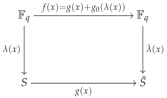
Niu et al. [30] studied the compositional inverse of the permutation polynomial in Lemma 5 using the commutative diagram method. An alternative proof of their result, based on the local method, is also available and leads to the following conclusion.
Theorem 33.
[30] [Theorem 16] Let the notations be defined as in Lemma 5. Let be a permutation over and be the compositional inverse of over Then the compositional inverse of is
Proof.
Since we have
by Theorem 7. Let
Then by , we have or
It follows from Theorem 14 that the compositional inverse of of is
This completes the proof. □
Remark 4.
Theorem 33 shows that the requirements in Lemma 5-namely, that S and are subsets of with , and that is an additive map satisfying for all —are imposed to construct a mapping satisfying . However, these very conditions also restrict the possibility of generalizing permutation properties for such polynomials. Furthermore, the purpose of imposing these two conditions, along with the requirement that is a bijection from S to , is essentially to show that can be represented as a composition of a certain function with .
Following the first class, the second type of permutation polynomials of the same form and their compositional inverses have also been studied in existing literature. To contextualize the subsequent discussion, the explicit compositional inverses of permutation polynomials involving a b-linear translator are presented. Both examples below are concerned with the notion of a b-linear translator.
For , and a mapping , is referred to as a b-linear translator [10,36,37] of with respect to S if for all and .
The following result characterizes when is a permutation polynomial.
Lemma 6.
[10] [Theorem 6.4] Let and be surjective map. Let be a linear translator with respect to S for the map Then for any which maps S into we have that is a permutation polynomial of if and only if permutes
It can be illustrated by the following commutative diagram.
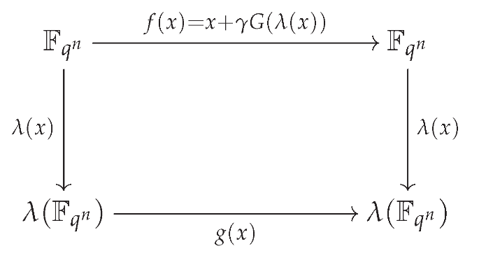
Niu et al. [30] derived the compositional inverse of permutation polynomials in Lemma 6 by means of commutative diagrams. In this work, we provide a more concise and intuitive proof via the local method.
Theorem 34.
[30] [Theorem 27] Let the notations be defined as in Lemma 6. Assume that is a permutation polynomial over and is the compositional inverse of Then the compositional inverse of is given by
Proof.
We have by assumption. Next, applying Theorem 7, we deduce
Take
in Theorem 14, then we arrive at
Consequently, the compositional inverse of over is expressed as
in view of Theorem 14. This is the desired result. □
Remark 5.
Theorem 27 in [30] establishes that the compositional inverse of is
However, this expression can be simplified. Recalling that we find that
which implies that the terms vanish identically. Therefore, the inverse simplifies to
When , the compositional inverse of is provided in [38] [Proposition 4] as , where p denotes the characteristic of .
Another important class arises when G is taken as the identity, i.e., . The core framework of [37] for establishing the permutation property and the inverse relies on the notion of linear translators and iterative composition of the permutation f. Specifically, the authors first leveraged the properties of linear translators to construct this class; they then conducted a detailed analysis of the cycle structure of f, and ultimately deduced the explicit expression of the compositional inverse.
Below, we provide a new proof of their result using the local method.
Theorem 35.
[37] [Theorem 3] Let be a b-linear translator of and . Then is a permutation polynomial of . Moreover, its inverse is given by .
Proof.
Since is a b-linear translator of , we have
If , then is not a permutation polynomial over Now we assume that Taking and we have
It follows from Theorem 14 that the compositional inverse of is
This completes the proof □
The research on permutation polynomials of the form over originated from [36,39], where , , and . A sufficient and necessary condition for to be a permutation polynomial over was established in [39,40]. Additionally, if is a permutation polynomial over and for some integer with , its compositional inverse is given in [40] [Theorem 4] as , where r is the multiplicative inverse of s modulo .
By [40] [Theorem 3], the permutation property of is equivalent to that of , where is a 0-linear translator (i.e., ) of . Therefore, this conclusion can be regarded as a special case of Theorem 35.
An application of the local criterion and the local method allows us to present the following generalization of Lemma 5, which also unifies Theorems 33 and 34. We omit the detailed proof as it closely follows the arguments in Theorem 33.
Theorem 36.
Let be polynomials. Suppose there exists a polynomial over such that Then the polynomial
permutes if and only if is injective on for each
In particular, if and are permutation polynomials over , let denote the compositional inverse of over Then the compositional inverse of over is given by
Remark 6.
It should be noted that the conclusion of Theorem 36 is derived from the Local Criterion applied to polynomials of the form . Meanwhile, Theorem 3.4 in [12] obtains exactly the same characterization based on the AGW Criterion if is permutation polynomial over .
3.5.2. Inverses of the Permutation Polynomials of the Form where is not a permutation polynomial
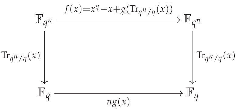
Different from the foregoing two families of the form , where itself acts as a permutation polynomial, the third family adopts . Clearly, is not a permutation polynomial over , since it is an -linear polynomial possessing a non-trivial kernel. Nevertheless, Yuan [16] conducted systematic research on polynomials of the form
where and is an integer. As will be seen in the theorem below, is a permutation polynomial over if and only if and g is invertible over
The main result in [16] was proved using the Local method. Here, we merely present the core function pairs required for the application of Theorem 14. Concretely, one may choose the paired functions
Combining with the inherent equalities
Yuan derived the desired result.
Theorem 37.
[16] [Theorem 4.2] Let be a positive integer, q a prime power and . Then the polynomial
is a permutation polynomial over if and only if and is a permutation polynomial over . Under such circumstances, let stand for the compositional inverse of g; then the compositional inverse of is given by
The commutative diagram for the above permutation polynomial is as follows.
3.6. Inverses of the Permutation Polynomials of the Form
In this subsection, we summarize the known results on the compositional inverses of permutation polynomials of the form
Depending on whether or , the structure of the compositional inverse exhibits distinct features. We therefore discuss these two cases separately.
3.6.1. Inverses of the Permutation Polynomials of the Form
We now present known results on the compositional inverses of permutation polynomials of the form
over , where are additive polynomials, is arbitrary, and satisfies certain conditions.
Two main research streams have emerged for this class of polynomials. The first stream focuses on the case where and , with various choices of g (e.g., , , or ) and additive [35,41,42,43,44,45,46,47,48,49,50,51,52,53,54,55,56,57,58,59,60,61,62,63,64]. The second stream considers as the trace function from to (or the absolute trace when the base field is a prime field), with and [65,66,67], or more generally, where is additive [68].
Akbary et al. [10] investigated the permutation properties of polynomials of the form (8) using the AGW criterion and established the following result.
Theorem 38.
[10] [Theorem 5.1] Let be additive polynomials and be a q-polynomial satisfying and . Let be any polynomial such that , and let be any polynomial. Then
permutes if and only if
(i) and
(ii) is a bijection from to
The commutative diagram for the above permutation polynomial is as follows.
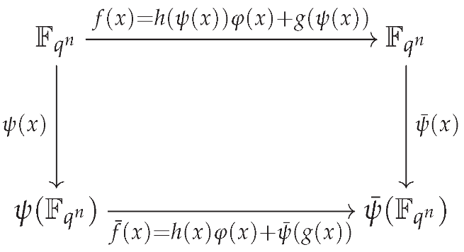
In the following content, we summarize the existing results on compositional inverses of permutation polynomials of the form given in Theorem 38. We do not provide new proofs for these known conclusions via the local method, and the main reasons are explained in the final paragraph of this subsection.
We first introduce the earliest relevant research outcome. Tuxanidy and Wang [69] studied the compositional inverses of the permutation polynomials in Theorem 38 by the decomposition method. This method is inspired by Wu and Liu [70]. Wu and Liu considered the compositional inverse of a class of bilinearized PPs over , i.e., , where q is even, n is odd, is a bilinear permutation polynomial over for a linearized polynomial (we also derive the compositional inverses of such polynomials via the local method in this paper, see Theorem 48 for details). The idea of the decomposition method mainly consists of the following two steps. First, the finite field is decomposed into the direct sum by the map Second, based on this decomposition, the problem of computing the inverse of can be converted into the problem of computing the inverse of a bivariate function that permutes This in turn is equivalent to obtaining the inverses of two permutation polynomials over the subspace and respectively, thus simplifying the original problem into two more manageable sub-problems.
The key step in extending this useful idea to computing the compositional inverse of permutation polynomials in Theorem 38 is to extend into arbitrary linearized polynomial . However, even though and hold, they still may not have a "nice enough" expression for Tuxanidy and Wang [71] instead use the map where is a subspace of in similarity with as above. Thus, to calculate the inverse of in Theorem 38, they had to add the conditions and and got the following result.
Theorem 39.
[71] [Theorem 1.2] Using the same notations and assumptions of Theorem 38, assume that is a permutation of , and further assume that and Then φ induces a bijective from to Let , induce the inverses of and , respectively. Then the compositional inverse of over is given by
Furthermore, if φ induces a bijection from to then φ permutes and the compositional inverse of over is given by
For several explicit families of permutation polynomials deduced from Theorem 39 in [71], we omit the detailed expressions of their compositional inverses and will not enumerate them individually. Instead, we mainly survey relevant results on compositional inverses for permutation polynomials of the form from existing literature.
Under the conditions , and (where are positive integers such that , and ), Niu et al. [34] applied the commutative diagram method to determine the compositional inverse of the permutation polynomial of the form over , obtaining the following result.
Theorem 40.
[34] [Theorem 3.7] Let q be a prime power, be positive integers with , , and such that permutes where Assume is the compositional inverse of . Then for any , is a permutation polynomial over and the compositional inverse of over is
The commutative diagram for the above permutation polynomial is as follows.
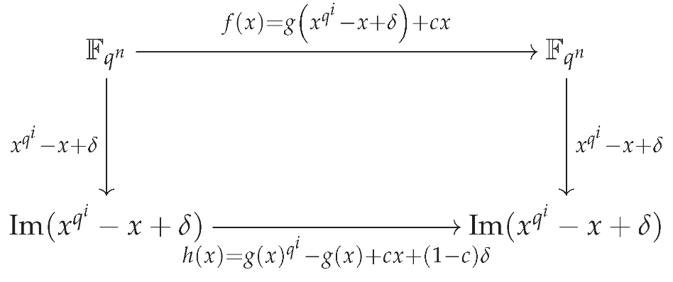
Remark 7.
By virtue of the relationship between affine q-polynomials and additive polynomials, Theorem 40 is merely a special case of Theorem 39.
Next, we present the second research result in this line of work. In 2021, Reis and Wang [72] investigated the compositional inverses of permutation polynomials of the form (8) under more specific conditions. Specifically, they explored the compositional inverses when and is the linearized q-associate of with . Recently, Reis and Wang [73] refined their results by studying as the q-associate of with and with By using the AGW criterion, the compositional inverse of was transformed into the compositional inverse of a certain related function over the sub-field, and thus the compositional inverse of was constructed. They gave the following result.
Theorem 41.
[73] [Theorem 3.2] Let be defined as before and δ be a nonzero root of . Let The polynomial
with and is a PP if and only if the following conditions holds:
(1)
(2) is a PP over where and s are the coefficients of f in
In affirmative case, if is the inverse of over then the inverse PP of over is given by
where and are given as follows:
(i) if then is the unique polynomial of degree at most such that and F is any polynomial satisfying
(ii) if then is the unique polynomial of degree at most such that and F is any polynomial satisfying where
The commutative diagram for the above permutation polynomial is as follows.
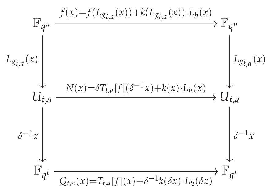
Remark 8.
Let , , , , and take , which is a nonzero root of . Set , and in Theorem 41. Then we have and , so that
is a permutation polynomial over according to Theorem 41.
Furthermore, we have
which implies that the intersection contains nonzero elements.
This example verifies that the condition in Theorem 39 fails to hold in this case. Consequently, Theorem 41 cannot be regarded as a special case of Theorem 39.
The authors also have established the compositional inverses for several classes of permutation polynomials where, in the setting of Theorem 41, acts as a trace function and . This work represents a shift toward a direct computational paradigm using the local method, in contrast to the approach in Theorems 39, 40, and 41, which typically relies on constructing and verifying a candidate polynomial. Specifically: In [74], the authors explicitly derive the compositional inverses for permutation polynomials of the form over .
In [75], this constructive approach is extended to the more general family of polynomials over , which is of the form , where , and satisfies the following two key conditions: (i) for some polynomial over ; (ii) for any , is injective on the fiber . Rather than relying on verification after construction, these papers shift the focus toward systematic derivation via this local method, offering explicit expressions for the inverses.
An additive analogue of the index of a univariate polynomial over a finite field was introduced by Reis and Wang [76]. We can also write an arbitrary polynomial uniquely according to its additive index. Namely, where are p-linearized polynomials over splits completely over and L is of the maximal degree. In this case, the additive index of f is which is the index of the kernel of L as subgroup of the additive group of
Definition 9.
Let and be an -vector space of dimension Then can be partitioned into where each is of the form with For a p-linearized polynomial and a sequence in we can define an M-affine mapping P of index with the subspace by
We observe that each branch function ia sn affine polynomial and thus we can obtain the inverse of by putting together the inverses of branch functions. The following result provides an implicit way of obtaining the inverse of a PP based on its additive decomposition as
Theorem 42.
[76] [Theorem 5.8] Let L be a monic p-linearized polynomial that divides set and Let be any complete set of representatives for the quotient Suppose that is a PP of where M is a p-linearized polynomial. Then is the inverse PP of over where and are given as follows:
(i)
(ii) is the unique p-linearized polynomial of degree at most such that for every
(iii) is the unique polynomial of degree at most such that
In particular, the additive indices of and coincide.
An application of the local criterion and the local method allows us to present the following generalization of Lemma 5, which also unifies Theorems 33 and 34. We omit the detailed proof as it closely follows the arguments in Theorem 33.
Theorem 43.
Let be polynomials, and let be additive polynomials over such that Assume that
is a polynomial over If there exists a polynomial such that then permutes if and only if
Remark 9.
Based on Lemma 7, the condition in Theorem 38 that is a bijection from to implies a key relationship among the maps. Specifically, for all , we have the functional identity
where is the inverse of . Furthermore, by Theorem 11, is a permutation polynomial over if and only if for every , the function is injective on the preimage set , and this injectivity condition is equivalent to
Employing the local method, the authors have fully solved the construction problem of the compositional inverse of permutation polynomials in Theorem 43. This method avoids utilizing the direct-sum decomposition of finite fields, and the corresponding research findings are in preparation for publication.
3.6.2. Inverses of the Permutation Polynomials with
We consider the following generalized form of which is given by
Yuan [35] generalized Theorem 38 and proved the following theorem, which gives a uniform treatment of some earlier constructions of permutation polynomials and also new permutation polynomials.
Theorem 44.
[35] [Theorem 3.1 ] Let q be a prime power, and let and be positive integers. Let be q-polynomials, , and such that and . Then
is a permutation polynomial of if and only if
(1) permutes ; and
(2) for any , permutes .
We generalize the result by the local criterion and get the following result.
Theorem 45.
Let q be a prime power and be positive integers. For let be additive polynomials. For if there exsits a polynomial such that , then the polynomial
permutes if and only if for any permutes
Remark 10.
The compositional inverse computation approach established in Theorem 43 is applicable to the permutation polynomial constructed in Theorem 45. This enables us to derive an explicit preimage formula for arbitrary elements under , which further extends the conclusion of Theorem 3.10 in [71].
For permutation polynomials of this category, we omit separate listings if only preimage representations rather than closed-form compositional inverses are obtainable. Currently, relevant findings on compositional inverses of such permutation polynomials remain limited, and all existing achievements are established via the direct sum decomposition method [9,69,71]. The local method proposed in this subsection can universally verify all reported results in this field.
Accordingly, this subsection does not enumerate all available cases exhaustively. we briefly review the research progress on compositional inverses of this type of permutation polynomials in a specific subclass, and adopt the local method to provide new proofs for the latest published results, while other cases are not discussed separately (they can be proved by similar methods). Based on the above considerations, we focus on a special class concerning compositional inverses and provide new proofs for the most recent results.
We first revisit the explicit inverse formula given by Coulter and Henderson for a family of bilinear permutation polynomials over finite fields of characteristic two (Theorem 46).
Theorem 46.
[77] [Theorem 1] Let , let n be odd, and let . Then the inverse of the PP over is as follows.
For , let
Set
and
Then is the inverse of over .
Laigle-Chapuy [78] generalized the construction of the permutation in Theorem 46 in a recursive manner to obtain the permutation (47).
Theorem 47.
[78] Let q be a power of 2 and n be odd. Assume is a bilinear permutation polynomial over for a linearized polynomial . Then the polynomial
As observed by Wu [70], Theorem 47 indeed generalizes Theorem 46: by setting and for some in , one easily verifies that
where is the permutation polynomial in Theorem 46. Wu [70] also gave the compositional inverse of by the decomposition method.
Theorem 48.
[70] Use the same notations as in Theorem 2.2 and let for a positive integer m. Assume the compositional inverse of is . Then
Tuxanidy and Wang, building upon their results in [71](which were also obtained via the direct sum decomposition), further generalized the conclusion of Wu [70].
Theorem 49.
[69] [Theorem 3.3, Corollary 4.3] Let be a power of a prime number p, let , and let be positive integers such that and . Then
is a complete permutation polynomial over for each if and only if is a complete permutation polynomial over . Moreover, If the polynomial f in Theorem 3.3 is a permutation polynomial over , then its compositional inverse over is given by
where and is the compositional inverse of over
Since the proofs of Theorem 47, Theorem 48, and Theorem 49 follow the same line of reasoning, we only present a detailed proof of Theorem 48 by way of illustration via the Local method. We adopt the following notation . For notational convenience, we denote the compositional inverse of the restricted mapping by , that is, .
Proof of Theorem 48
Firstly, it is obvious that
which implies that
where is the inverse of over Moreover, we have
Define the set and
If , then this yields
If , we define One can verify that . Substituting the identity into the expression of , we get
Then by (11)
Hence, we have
It follows from Theorem 14 that
In the proof of Theorem 48 constructed using the local method, it becomes evident that we do not need to rely on direct sum decompositions to solve for the compositional inverse of
3.7. Inverses of Permutations of the Form , where Are Additive Polynomials
In this subsection we consider the problem of explicitly constructing the compositional inverse of permutation polynomials of the form
where each is a linearized polynomial over whose image is a 1-dimensional -vector space.
As a transitional statement, we first assume that the sets (where the index i runs over a suitable collection) are pairwise orthogonal.
Let be a positive integer, q a prime power satisfying , and a primitive d-th root of unity over . We recall the definition of a family of polynomials introduced in [16]:
This family of polynomials enjoys three fundamental properties that are central to the study of permutation polynomials (PPs) over finite fields. These properties are summarized below:
(i) For each , satisfies .
(ii) For any positive integer m and any indices , the composition of with is given by:
(iii) For any integer and any polynomial , the composition vanishes identically over .
Now let be positive integers, , and . In [16], Yuan considered polynomials of the form:
The permutation behavior of can be illustrated by the following commutative diagram:
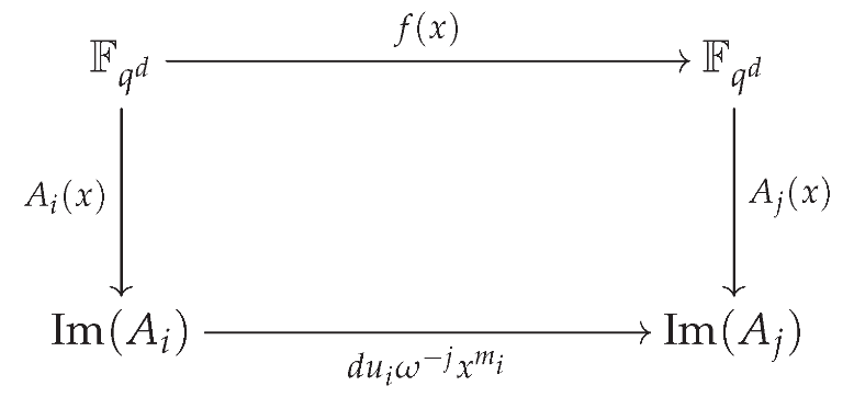
If , then the compositional inverse of the monomial is , where is the positive integer satisfying . This gives rise to the following commutative diagram:
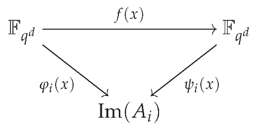
where for , , and for .
We also recall the standard decomposition identity:
Combining these commutative diagrams and the decomposition identity, Yuan [16] established the following result.
Theorem 50.
[16] [Theorem 4.1] The polynomial is a PP over if and only if the following conditions hold:
(1) is a complete residue modulo d;
(2) ;
(3) ;
(4) is a PP over .
Furthermore, if is a PP over let be positive integers with and let be the compositional inverse of Then the compositional inverse of is
Remark 11.
Let be as defined in Theorem 50. In [14] [Theorem 5.3], Yuan et al. gave a full characterization of permutation polynomials over of the form with . This characterization is a special case of Theorem 50.
Next, we turn to cases where the orthogonality condition is not satisfied. The first such example was given by Wu and Yuan [79], who studied a class of PPs of the form and their inverses over using the local method.
Theorem 51.
[79] [Theorem 2] Let q be a prime power and m be a positive integer. Assume that with , and Then the polynomial
is a permutation polynomial over if and only if and the compositional inverse of is
where , and
In this case, and . Moreover, .
The second example concerns permutation polynomials over of the form
By direct computation and under the assumption that (which will appear as a necessary and sufficient condition in the theorem below), Yuan[14] obtain the following two commutative diagrams:
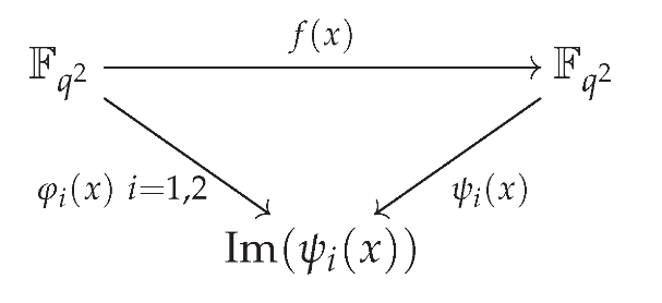
where
If , then there exist positive integers such that
It follows that
and consequently,
Yuan[14] got the following characterization.
Theorem 52.
[14] [Theorem 5.5] Let q be a prime power, and let be two elements of order in . Then the polynomial , where , is a permutation polynomial of if and only if and .
Building on the idea of Yuan [14], Wu and Yuan [79] generalized Theorem 52. Here we do not present the proof details, but only give the necessary notation and the result.
We give some notations at first. Let q be a prime power and be a positive integer. For a positive integer i with , assume that with and the polynomial
Let be positive integers and Put
Let and
Then the authors have the following results by applying the local method.
Theorem 53.
[79] [Theorem 3] Let q be a prime power and be a positive integer. And let the notations , , and be as above. Assume that are positive integers and Then the polynomial
is a permutation polynomial over if and only if and the determinant of is not Moreover, if is a PP over then
where is the th row of and is the last row vector of
Based on Theorem 53, six new classes of permutation polynomials of the form over are constructed in [80]; we do not list them in detail here.
As we well know, the vector space and the finite field are isomorphic as -vector spaces, and therefore every permutation of can be equivalently represented as a PP over .
Let and be a pair of dual bases of over , and let be a polynomial. Then for any , with we defined
It is easy to see that are well-defined and are uniquely determined by and the base Moreover, we have
Theorem 54.
[81] [Theorem 1.2] If is a PP over and are maps from to then the polynomial
where are defined above, is a PP over if and only if the following two conditions hold:
(i) is a base of over
(ii) are PPs over
Moreover, if and are the compositional inverses of and respectively, and is the dual base of , then we have
As a consequence of Theorem 54, Yuan [81] gave the following results.
Corollary 5.
[81] [Corollary 1.1 ]Let be n elements of over , and let
Then is a over if and only if the following three conditions hold
(i) ,
(ii) is a basis of over .
(iii) is a basis of over .
Remark 12.
The following characterization of linear permutation polynomials over finite fields is established in [82].
(1) Let be any given basis of over , and let be a linear polynomial over . Then there exist n elements such that
Moreover, is a permutation polynomial if and only if forms a basis of over . There are exactly distinct linear permutation polynomials, all of which admit the above representation with a basis .
(2) Let be any given basis of over , and let
Then is a permutation polynomial if and only if is a basis of over .
With the aid of this result, one can observe that Theorem 54 actually generalizes the results given in Theorem 50, 51, Theorem 52 and Theorem 53.
In [36], Charpin and Kyureghyan characterized and constructed permutation polynomials of the form where . Moreover, they proposed the following problem.
Problem 1.
[36] [Open Problem 1] Characterize a class of permutation polynomials of type , where is neither a permutation nor a linearized polynomial.
Theorem 55.
[81] [Theorem 4.1] If is a polynomial such that is not a constant map, , then there are at least permutation polynomials of the form
such that is neither a permutation nor a linearized polynomial.
In 2008, Charpin and Kyureghyan [83] studied permutation polynomials of the form over finite fields with even characteristic using linear structures, and obtained six classes of such permutations. They [36] subsequently generalized this work to finite fields with odd characteristic. Meanwhile, in [37], Kyureghyan also constructed large families of permutation polynomials of the form , where is an -linear permutation over .
Theorem 56.
[37] [Theorem 1] Let , be arbitrary mappings. Let be an -linear permutation of . If , and is a b-linear translator of f, then
permutes if and only if permutes .
Pang et al. [84] provide the following definition of linear translators, which is somewhat different from [10,36,37].
Definition 10.
[84] [Theorem 3.4] Let , and be an additive permutation polynomial over . A non-zero element is called a -linear translator of the function f if
holds for any and a fixed .
Let or be an additive permutation polynomial over in the following two results.
Pang et al. [84] give a generalized result for permutations of in [85] and [86] based on Definition 10 and give their compositional inverses.
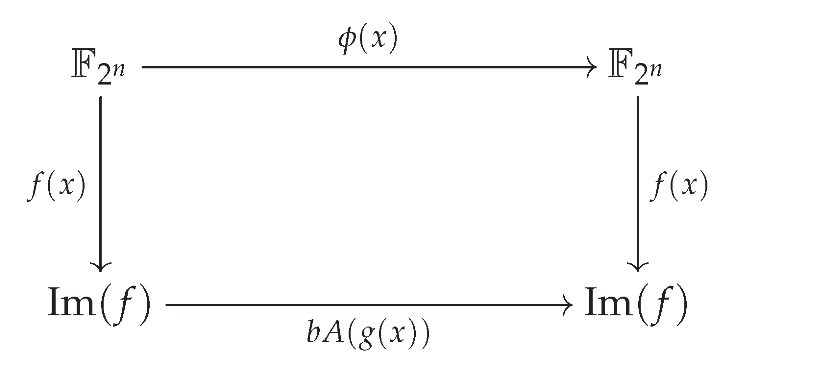
Theorem 57.
[84] [Theorem 3.1 ] Let be an arbitrary mapping, and an -linear permutation of . Let be a permutation of , and the compositional inverse of . If is a -linear translator of f, then
is a permutation polynomial over , and its compositional inverse is
The commutative diagram for the permutation polynomial is as follows:
Using the classic definition of linear translators, Qin and Yan [87] [Theorem 2.1] constructed a class of permutation polynomials of the shape
Pang et al. [84] show an analogous result with minor modifications and give its compositional inverse.
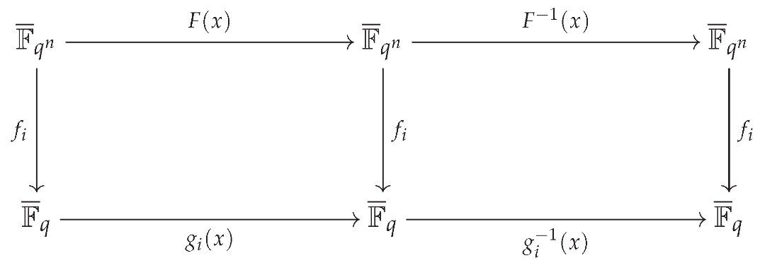
Theorem 58.
[84] [Theorem 3.3] Let , . Let , and be linearly independent over . If is a -linear translator of for , and a -linear translator of when , then
is a permutation polynomial over if and only if is a permutation polynomial over , where . Moreover, the compositional inverse of is given by
The commutative diagram for the permutation polynomial is as follows:
3.8. Inverses of Piecewise-Constructed Polynomials
The Lagrange interpolation formula is well known for calculating polynomial expressions in a point-to-point manner. For any , applying the one-variable Lagrange interpolation formula, we can write the polynomial as the linear combination
where and . According to the Lagrange interpolation formula, its inverse can be expressed as
The basic idea of piecewise constructions of PPs is to partition a finite field into subsets and study the permutation property via the functions’ behavior on these subsets. This idea, summarized in [88] by Cao, Hu and Zha, also applies to finite rings.
The following lemma provides a more general piecewise description of polynomials over finite fields.
Lemma 7.
[88] [Proposition 3] Let be a partition of , and let . Define
where is the characteristic function of , i.e., if and otherwise. Then is a permutation polynomial (PP) of if and only if
(i) is injective on for each ; and
(ii) for all .
From the perspective of construction principles and application purposes, the piecewise method shares similarities with the Lagrange interpolation formula. In this sense, the piecewise method can be viewed as a generalized form of the Lagrange interpolation formula. Specifically, when each is a singleton set, the piecewise expression reduces exactly to the standard Lagrange interpolation formula. Inspired by the lemma above, Zheng et al. [89] present the following piecewise interpolation method for constructing inverses of all PPs of finite fields.
Theorem 59.
where for any and is the characteristic function of
According to the above lemma, to obtain the compositional inverse of , we need to accomplish the following two steps: (1) for each i, compute the local inverse map of restricted to , satisfying for any ; and (2) derive an explicit expression for the characteristic function . We only introduce one typical example of piecewise permutation polynomial along with its compositional inverse based on Theorem 59, which is presented as follows.
Let be a fixed primitive element of and a fixed primitive l-th root of unity. Let and the set of all nonzero l-th be Then is a subgroup of of index The elements of the factor group are the cyclotomic cosets
For any and a positive integer r, the r-th order cyclotomic mapping of index l from to itself (see Niederreiter and Winterhof [90] for or Wang [32] for general r ) is defined by
Clearly, an r-th order cyclotomic mapping of index l produces a polynomial of the form where Indeed, the polynomial representation of (16) is given by
More generally, a simple class of generalized cyclotomic mapping PPs of was defined in [91] as
Several equivalent criteria for f permuting were given in [91], and one is that is a PP of if and only if and In fact, the polynomial defined in (18) can be rewritten as
Because each branch function is a monomial that maps one coset to another, it is straightforward to find its inverse, which is also a monomial. Putting them together, we obtain the compositional inverse of .
Theorem 60.
is given by
where and
A more generalized notation of coset-wise affine permutation functions and their cycle types were studied in [93]. The most general piecewise construction of permutations using characteristic functions of any partition of a finite field was summarized in [88,94]. Piecewise constructions of inverses of these piecewise PPs were also studied in [89,92,95].
3.9. Coefficients of Inverses of General Permutation Polynomials
In the following, we present two different methods for studying inverse permutation polynomials. The first approach, based on matrix representation, reduces polynomial composition and inversion to matrix multiplication and matrix inversion; the second approach, by contrast, employs the orthogonality of the discrete Fourier transform to express the coefficients of the inverse polynomial as weighted sums of the values of the original polynomial.
3.9.1. Method 1: Matrix Representation
Let be the finite field of order where p is a prime number and n is a positive integer. Let be a polynomial over with degree at most . To compute its composition with another polynomial , we can either use interpolation to obtain its expression directly, or calculate all the powers in the expression .
Denote by
the k-th power of the polynomial for . Denote by the zero polynomial in . If we will define and .
For any polynomial we associate a coefficient vector with it, namely,
A matrix associated with is defined by
where the k-th column consists of the coefficients of the -th power of . With this matrix notation, the composition of polynomials admits a remarkably simple algebraic description.
Theorem 61.
[96] Let and . Let be the composition of g with f. Then
In the special case where f is a permutation polynomial, its compositional inverse also admits a simple expression in terms of this matrix.
Theorem 62.
[96] Let f be a permutation polynomial of . Let P be the antidiagonal permutation matrix, i.e. P is defined by for and zero otherwise. Then
3.9.2. Method 2: Discrete Fourier Transform Method
The orthogonality of the discrete Fourier transform over finite fields provides a weighted-sum representation for the coefficients of the inverse polynomial.
Let be a permutation polynomial (PP) of and let be its inverse modulo . For each , it is well known that
Since is a permutation polynomial of , we have
Set
Then
Therefore, finding any coefficient of the inverse is equivalent to finding the coefficient of in the expansion of the power . The following theorem, is a direct consequence of this observation and provides an explicit formula for the coefficients of the inverse in a special but important class of permutation polynomials.
Theorem 63.
[97] Let be a permutation polynomial of , where , , , and . Denote by
the inverse polynomial of modulo . Then the following hold.
(i) There are at most ℓ nonzero ’s such that , where and .
(ii) Let . Then
where ω is a primitive ℓ-th root of unity.
(iii) Let
and let . Then if and if
Although we present explicit coefficient formulas for compositional inverses of permutation polynomials within this section, these identities are of limited utility in practice. For arbitrary q, one cannot extract concrete closed-form expressions for individual coefficients directly from the given formulas.
3.10. Compositional Inverses of Known Permutation Polynomials Not Obtained from the AGW Criterion
The local method is a valuable tool for constructing permutation polynomials over finite fields and for calculating their composition inverses. In the past, we often demonstrated that a polynomial is a permutation over by using the equation (any ), which has at most one solution in . If we can identify the unique solution of the equation as we can then utilize local methods to derive the composition inverse of as . We present the composition inverses for trinomials and quartics at first.
We introduce the resultant of two polynomials.
Definition 11.
Let and be two polynomials of degree n and m, respectively, with Then the resultant of the two polynomials with respect to x is defined by the determinant
of order
If where in the splitting field of f over then is also given by the formula
Then if and only if f and g have a common divisor in of positive degree.
Definition 12.
[98] [Definition 2.2] Two permutation polynomials and in are called quasi-multiplicative (QM, for short) equivalence if there exists an integer with and , where .
The following three results were initially established by Gupta et al. [99] through the multivariate method and polynomial resultants. While Wu et al. [100] confirmed these results using the local method, their work also provided the explicit compositional inverses of the permutation polynomials.
Theorem 64.
[100] [Theorem 3.1] For a positive integer m, let and with Then the polynomial is a permutation polynomial over if and only if Moreover, if is a permutation polynomial over , then the compositional inverse of is
Remark 13.
Based on the character function of finite field , the inverse function originally defined in piecewise form can be converted into an integrated algebraic expression without segmented judgment, whose specific formula is given by
On this basis, setting in Theorem 64 yields the permutation polynomial . This polynomial is consistent with the research object described in Theorem 2.3 of [101]. Furthermore, Gupta et al. pointed out in Corollary 3.3 of [99] that possesses QM equivalence with permutation polynomial . The equivalence holds under the condition , satisfying the relation . It is also found that the research findings of can generalize the theoretical results proposed in Theorem 3.1 of [102]. For the above reasons, we will not repeat the derivation of compositional inverses for polynomials involved in the two aforementioned classic theorems.
Theorem 65.
[100] [Theorem 3.2] For a positive integer m, let and with Then the polynomial is a permutation polynomial over if and only if Moreover, if permutes , then the compositional inverse of is
Remark 14.
Setting in Theorem 65 yields the permutation polynomial which corresponds to Theorem 4.3 in [103]. This polynomial is QM-equivalent to another permutation polynomial, , as established in [99] [Corollary 3.5] via the relation (given ). The polynomial itself generalizes the one presented in Theorem 3.2 of the earlier work [102]. Therefore, the compositional inverses for the polynomials in Theorem 4.3 of [103] and Theorem 3.2 of [102] are not reiterated here.
Theorem 66.
[100] [Theorem 3.3] Let q be a prime power and . Then the polynomial
is a permutation polynomial over if and only if Moreover, if permutes , the compositional inverse of is
Employing the same multivariate and resultant techniques, Wang et al. [104] established the following six related results.
Theorem 67.
[104] [Theorem 3.1] For a positive integer k with Let Then
is a permutation polynomial over
Wang et al. [104] showed that for any , if then the unique solution of is and if then the unique solution of is
where Applying the local method, we have the following result.
Theorem 68.
Let the notations be defined as Theorem 67. Then the compositional inverse of over is
Theorem 69.
[104] [Theorem 3.2] For a positive integer k with Let Then
is a permutation polynomial over
Wang et al. [104] showed that for any , if then the unique solution of is and if then the unique solution of is
where Using the local method, we have the following result.
Theorem 70.
Let the notations be defined as in Theorem 69. Then the compositional inverse of over is
Theorem 71.
[104] [Theorem 3.3] For a positive integer k with Let Then
is a permutation polynomial over
Wang et al. [104] showed that for any , if then the unique solution of is and if then the unique solution of is
where According to the local method, we have the following result.
Theorem 72.
Let the notations be defined as in Theorem 71. Then the compositional inverse of over is
Theorem 73.
[104] [Theorem 3.4] For a positive integer k with Let Then
is a permutation polynomial over
Wang et al. [104] showed that for any , if then the unique solution of is and if then the unique solution of satisfies
or
where According to the local method, we have the following result.
Theorem 74.
Let the notations be defined as in Theorem 73. Then the compositional inverse of over is
Theorem 75.
[104] [Theorem 3.5] For a positive integer k with Let Then
is a permutation polynomial over
Wang et al. [104] showed that for any , if then the unique solution of is and if then the unique solution of is
where It follows from the local method that we have the following result.
Theorem 76.
Let the notations be defined as in Theorem 75. Then the compositional inverse of over is
Theorem 77.
[104] [Theorem 3.6] For a positive integer k with Let Then
is a permutation polynomial over
Wang et al. [104] showed that for any , if then the unique solution of is and if then the unique solution of is
where It follows from the local method that we have the following result.
Theorem 78.
Let the notations be defined as in Theorem 77. Then the compositional inverse of over is
Theorem 79.
[105] [Theorem 2] For a positive integer m, let and If m is even with and then
is a permutation polynomial over
Pang et al. [105] showed that for any , if then the unique solution of is and if then the unique solution of is
where It follows from the local method that we have the following result.
Theorem 80.
Let the notations be defined as in Theorem 79. Then the compositional inverse of over is
Theorem 81.
[105] [Theorem 3] For a positive integer m, let and If m is even with and then
is a permutation polynomial over
Pang et al. [105] showed that for any , if then the unique solution of is and if then the unique solution of is
where It follows from the local method that we have the following result.
Theorem 82.
Let the notations be defined as in Theorem 81. Then the compositional inverse of over is
Theorem 83.
[105] [Theorem 4] For a positive integer m, let and Then
permutes if one of the following conditions holds:
(1) , and
(2) with , and
(3) m is even, and
Pang et al. [105] showed that for any , if then the unique solution of is if then the unique solution of with condition (1) is
the unique solution of with condition (2) is
and the unique solution of with condition (3) is
where It follows from the local method that we have the following result.
Theorem 84.
Let the notations be defined as in Theorem 83.
(1) If , and then the compositional inverse of over is
(2) If with , and then the compositional inverse of over is
(3) If m is even, and then the compositional inverse of over is
Theorem 85.
[105] [Theorem 5] For a positive integer m with , let and with and Then
permutes
Pang et al. [105] showed that for any , if then the unique solution of is if then the unique solution of is
where It follows from the local method that we have the following result.
Theorem 86.
Let the notations be defined as in Theorem 85. Then the compositional inverse of over is
Theorem 87.
[105] [Theorem 6] For a positive integer m with , let and with and Then
permutes
Pang et al. [105] showed that for any , if then the unique solution of is if then the unique solution of is
where It follows from the local method that we have the following result.
Theorem 88.
Let the notations be defined as in Theorem 87. Then the compositional inverse of over is
Bartoli [106] considered four classes of permutation trinomials over
Let
Theorem 89.
[106] [Theorem 3.4] Let If then the polynomial
is a permutation polynomial of
Bartoli [106] showed that for any , if then the unique solution of is and if then the unique solution of is
Theorem 90.
Let the notations be defined as in Theorem 89. Then the compositional inverse of over is
Theorem 91.
[106] [Theorem 3.5] If with and are such that has no roots in then the polynomial
is a permutation polynomial of
Bartoli [106] showed that for any , if then the unique solution of is and if then the unique solution of is
Theorem 92.
Let the notations be defined as in Theorem 91. Then the compositional inverse of over is
Theorem 93.
[101] [Theorem 2.4] Let be positive integers with and Then
is a permutation polynomial over
Wang et al. [101] showed that for any , if then the unique solution of is and if then the unique solution of is
where It follows from the local method that we have the following result.
Theorem 94.
Let the notations be defined as in Theorem 93. Then the compositional inverse of is
Theorem 95.
[101] [Theorem 2.5] Let be positive integers Then
is a permutation polynomial over
Wang et al. [101] showed that for any , if then the unique solution of is and if then the unique solution of is
where It follows from the local method that we have the following result.
Theorem 96.
Let the notations be defined as in Theorem 95. Then the compositional inverse of over is
Theorem 97.
[98] [Proposition 2.6] Let be an odd integer and Then the polynomial
is a permutation polynomial over
As noted in [98], the permutation polynomial is **quasi-multiplicatively (QM) equivalent to the permutation polynomials in Theorems 5.1 and 5.2 of [107], namely:
and
Therefore, these results will not be restated here.
For any , Wu et al. [98] showed that the unique solution of the equation is
where Then we have the following result.
Theorem 98.
Let the notations be defined as in Theorem 97. Then the compositional inverse of over is
Lemma 8.
[108] [Theorem 3.4] Let k be a positive integer and q be a prime power with and let m be an even positive integer. Then
is a permutation polynomial of if and only if one of the following three conditions holds:
(1)
(2)
(3) and where denotes the exponent of 3 in cannonical factorization of
Ding et al. [108] have show that for any the equation has a unique root
and for the equation has the only solution Then we have the following result by Lemma 14.
Theorem 99.
Let the notations be defined in Lemma 8, and
is a permutation polynomial over Then the compositional inverse of is
For let . The following result is derived from the local method.
Table 2.
Known classes of non-linearized permutation trinomial over for odd characteristic and its inverse
Table 2.
Known classes of non-linearized permutation trinomial over for odd characteristic and its inverse
| No. | conditions on m and p | Refs. | its inverse | |
|---|---|---|---|---|
| 1 | , | [104] [Theorem 3.1] | Theorem 68 | |
| 2 | , | [104] [Theorem 3.2] | Theorem 70 | |
| 3 | , | [104] [Theorem 3.3] | Theorem 72 | |
| 4 | , | [104] [Theorem 3.4] | Theorem 74 | |
| 5 | , | [104] [Theorem 3.5] | Theorem 76 | |
| 6 | , | [104] [Theorem 3.6] | Theorem 78 |
Table 3.
Known classes of non-linearized permutation trinomial over and its inverse
| No. | Conditions on m | Refs. | Its inverse | |
|---|---|---|---|---|
| 1 | m is even | [105] [Theorem 2] | Theorem 80 | |
| 2 | m is even | [105] [Theorem 3] | Theorem 82 | |
| 3 | [105] [Theorem 4] | Theorem 84 | ||
| m is even | ||||
| 4 | [105] [Theorem 5] | Theorem 86 | ||
| 5 | [105] [Theorem 5] | Theorem 88 | ||
| 6 | with | [99] [Theorem 3.2] | Theorem 64 | |
| 7 | with | [99] [Theorem 3.4] | Theorem 65 |
Author Contributions
D. W. was responsible for the Conceptualization, visualization, and writing of the original draft. P. Y. contributed to the conceptualization and methodology design, provided research guidance, supervised the work. X.P. performed writing - review & editing of the manuscript. All authors have read and agreed to the published version of the manuscript.
Funding
This research was funded by the National Natural Science Foundation of China (NSFC) under Grant Nos. 12501006, 12171163 and 12571003.
Institutional Review Board Statement
Not applicable
Informed Consent Statement
Not applicable
Conflicts of Interest
The authors declare no conflicts of interest.
References
- Ding, C. Cyclic codes from some monomials and trinomials. SIAM Journal on Discrete Mathematics 2013, 27, 1977–1994.
- Ding, C.; Zhou, Z. Binary cyclic codes from explicit polynomials over GF(2m). Discrete Mathematics 2014, 321, 76–89.
- Laigle-Chapuy, Y. Permutation polynomials and applications to coding theory. Finite Fields and Their Applications 2007, 13, 58–70.
- Rivest, R.L.; Shamir, A.; Adleman, L. A method for obtaining digital signatures and public-key cryptosystems. Communications of the ACM 1978, 21, 120–126.
- Schwenk, J.; Huber, K. Public key encryption and digital signatures based on permutation polynomials. Electronics Letters 1998, 34, 759–760.
- Ding, C.; Yuan, J. A family of skew Hadamard difference sets. Journal of Combinatorial Theory, Series A 2006, 113, 1526–1535.
- Lidl, R.; Niederreiter, H. Finite fields; Number 20, Cambridge University Press: New York, 1997.
- Lidl, R.; Niederreiter, H. Introduction to finite fields and their applications; Cambridge University press: New York, 1994.
- Wang, Q. A survey of compositional inverses of permutation polynomials over finite fields. Designs, Codes and Cryptography 2025, 93, 831–870.
- Akbary, A.; Ghioca, D.; Wang, Q. On constructing permutations of finite fields. Finite Fields and Their Applications 2011, 17, 51–67.
- Yuan, P.; Pang, X.; Wu, D.; Guan, H. Injective Systems for Permutation Polynomials over Finite Fields. Frontiers in Combinatorics and Number Theory 2026, 2, 92–101. [CrossRef]
- Yuan, P. Compositional inverses of AGW-PPs -dedicated to professor cunsheng ding for his 60th birthday. Adv. Math. Commun. 2022, 16, 1185–1195. [CrossRef]
- Wan, D.; Lidl, R. Permutation polynomials of the form xrh(x(q-1)/d) and their group structure. Monatshefte für Mathematik 1991, 112, 149–163.
- Yuan, P. Permutation polynomials and their compositional inverses 2025. 32, 299–308.
- Rotman, J.J. An Introduction to the Theory of Groups, 4 ed.; Number 148 in Graduate Texts in Mathematics, Springer-Verlag: New York, 1995. [CrossRef]
- Yuan, P. Local method for compositional inverses of permutation polynomials. Communications in Algebra 2024, 52, 3070–3080.
- Wu, D.; Yuan, P. Permutation polynomials over finite fields by the local criterion, 2024, [arXiv:math.NT/2409.18758].
- Yuan, P.; Pang, X.; Wu, D. Algebraic Structure of Permutational Polynomials over Fqn II, 2025, [arXiv:math.NT/2503.22415].
- Pang, X.; Li, Y.; Yuan, P.; Zeng, Y. Determination of Some Types of Permutations over Fq2 with Low-Degree, 2025, [arXiv:math.NT/2508.01143].
- Lidl, R.; Mullen, G.L.; Turnwald, G. Dickson polynomials; Longman Scientific and Technical: Essex, 1993.
- Li, K.; Qu, L.; Wang, Q. Compositional inverses of permutation polynomials of the form xrh(xs) over finite fields. Cryptography and Communications 2019, 11, 279–298.
- Zheng, Y.; Wang, Q.; Wei, W. On Inverses of Permutation Polynomials of Small Degree Over Finite Fields. IEEE Trans. Inf. Theory 2020, 66, 914–922. [CrossRef]
- Zheng, Y.; Yu, Y.; Zha, Z.; Zhou, X. On inverses of permutation polynomials of the form x(xs-a)(qm-1)/s over Fqn. Designs, Codes and Cryptography 2023, 91, 1165–1181.
- Wu, B.; Liu, Z. Linearized polynomials over finite fields revisited. Finite Fields and Their Applications 2013, 22, 79–100.
- Coulter, R.; Henderson, M. A note on the roots of trinomials over a finite field. Bulletin of the Australian Mathematical Society 2004, 69, 429–432.
- Wu, B. Linearized and linearized derived permutation polynomials over finite fields and their compositional inverses. Ph. D. dissertation, Acad. Math. Syst. Sci., Chin. Acad. Sci., Beijing, China 2013.
- Wu, B. The compositional inverse of a class of linearized permutation polynomials over F2n, n odd. Finite Fields and Their Applications 2014, 29, 34–48.
- Tuxanidy, A.; Wang, Q. On the inverses of some classes of permutations of finite fields. Finite Fields and Their Applications 2014, 28, 244–281.
- Bastos, G.T. Linear permutations and their compositional inverses over Fqn. Journal of Algebra and Its Applications 2022, 21, 2250220.
- Niu, T.; Li, K.; Qu, L.; Wang, Q. Finding Compositional Inverses of Permutations From the AGW Criterion. IEEE Trans. Inf. Theory 2021, 67, 4975–4985. [CrossRef]
- Park, Y.H.; Lee, J.B. Permutation polynomials and group permutation polynomials. Bulletin of the Australian Mathematical Society 2001, 63, 67–74.
- Wang, Q. Cyclotomic Mapping Permutation Polynomials over Finite Fields. In Proceedings of the Sequences, Subsequences, and Consequences, International Workshop, SSC 2007, Los Angeles, CA, USA, May 31 - June 2, 2007, Revised Invited Papers; Golomb, S.W.; Gong, G.; Helleseth, T.; Song, H., Eds. Springer, 2007, Vol. 4893, Lecture Notes in Computer Science, pp. 119–128. [CrossRef]
- Zieve, M. On some permutation polynomials over F of the form xrh(x(q-1)/d). Proceedings of the American Mathematical Society 2009, 137, 2209–2216.
- Niu, T.; Li, K.; Qu, L.; Wang, Q. New constructions of involutions over finite fields. Cryptography and Communications 2020, 12, 165–185.
- Yuan, P.; Ding, C. Permutation polynomials over finite fields from a powerful lemma. Finite Fields and Their Applications 2011, 17, 560–574.
- Charpin, P.; Kyureghyan, G. When does G(x)+γTr(H(x)) permute Fpn. Finite Fields and Their Applications 2009, 15, 615–632.
- Kyureghyan, G.M. Constructing permutations of finite fields via linear translators. Journal of Combinatorial Theory, Series A 2011, 118, 1052–1061.
- Cepak, N.; Charpin, P.; Pasalic, E. Permutations via linear translators. Finite Fields and Their Applications 2017, 45, 19–42.
- Charpin, P.; Kyureghyan, G.M. Monomial functions with linear structure and permutation polynomials. In Finite Fields: Theory and Applications; American Mathematical Society: Providence, 2010; Vol. 518, Contemporary Mathematics, pp. 99–111.
- Charpin, P.; Kyureghyan, G.M.; Suder, V. Sparse permutations with low differential uniformity. Finite Fields and Their Applications 2014, 28, 214–243.
- Gupta, R.; Sharma, R. Further results on permutation polynomials of the form (xpm-x+δ)s+x over Fp2m. Finite Fields and Their Applications 2018, 50, 196–208.
- Helleseth, T.; Zinoviev, V. New Kloosterman sums identities over F2m for all m. Finite Fields and Their Applications 2003, 9, 187–193. [CrossRef]
- Hollmann, H.D.; Xiang, Q. Kloosterman sum identities over F2m. Discrete mathematics 2004, 279, 277–286.
- Li, G.; Cao, X. Several classes of permutation polynomials over the finite field Fp2m. Finite Fields and Their Applications 2023, 89, 102197. [CrossRef]
- Li, G.; Cao, X. Several classes of permutation polynomials based on the AGW criterion over the finite field F22m. Finite Fields and Their Applications 2024, 95, 102378. [CrossRef]
- Li, L.; Wang, S.; Li, C.; Zeng, X. Permutation polynomials (xpm-x+δ) s1+(xpm-x+δ) s2+x over Fpn. Finite fields and their applications 2018, 51, 31–61.
- Li, N.; Helleseth, T.; Tang, X. Further results on a class of permutation polynomials over finite fields. Finite Fields and Their Applications 2013, 22, 16–23.
- Liu, Q.; Jiang, R.; Zou, J. Several classes of permutation polynomials over Fp2m with odd characteristic based on the AGW criterion. Cryptography and Communications 2025, 17, 1569–1582.
- Tu, Z.; Zeng, X.; Jiang, Y. Two classes of permutation polynomials having the form (x2m+x+δ)s+x. Finite Fields and Their Applications 2015, 31, 12–24. [CrossRef]
- Tu, Z.; Zeng, X.; Li, C.; Helleseth, T. Permutation polynomials of the form (xpm-x+δ)s+L(x) over the finite field Fp2m of odd characteristic. Finite Fields and Their Applications 2015, 34, 20–35.
- Wang, L.; Wu, B. General constructions of permutation polynomials of the form (x2m+x+δ)i(2m-1)+1+x over F22m. Finite Fields and Their Applications 2018, 52, 137–155. [CrossRef]
- Wang, L.; Wu, B.; Liu, Z. Further results on permutation polynomials of the form (xpm-x+δ)s+L(x) over Fp2m. Finite Fields and Their Applications 2017, 44, 92–112. [CrossRef]
- Wu, D.; Yuan, P. Some classes of permutation polynomials of the form b(xq+ax+δ)i(q2-1)/d+1+c(xq+ax+δ)j(q2-1)/d+1+L(x) over Fq2. Applicable Algebra in Engineering, Communication and Computing 2022, 33, 135–149.
- Wu, D.; Yuan, P. Some new results on permutation polynomials of the form b(xq-ax+δ)s+ax over Fq2. Finite Fields and Their Applications 2024, 93, 102329.
- Xu, X.; Feng, X.; Zeng, X. Complete permutation polynomials with the form (xpm-x+δ)s+axpm+bx over Fp2n. Finite Fields and Their Applications 2019, 57, 309–343.
- Xu, G.; Luo, G.; Cao, X. Several classes of permutation polynomials of the form (xpm-x+δ)s+x over Fp2m. Finite Fields and Their Applications 2022, 79, 102001.
- Yuan, J.; Ding, C. Four classes of permutation polynomials of F2m. Finite fields and their applications 2007, 13, 869–876.
- Yuan, J.; Ding, C.; Wang, H.; Pieprzyk, J. Permutation polynomials of the form (xpm-x+δ)s+L(x). Finite fields and their applications 2008, 14, 482–493.
- Yuan, P.; Ding, C. Further results on permutation polynomials over finite fields. Finite Fields and Their Applications 2014, 27, 88–103.
- Zeng, X.; Zhu, X.; Hu, L. Two new permutation polynomials with the form (x2k+x+δ)s+x over F2n. Applicable Algebra in Engineering, Communication and Computing 2010, 21, 145–150.
- Zeng, X.; Zhu, X.; Li, N.; Liu, X. Permutation polynomials over F2n of the form (x2i+x+δ) s1+(x2i+x+δ) s2+x. Finite Fields and Their Applications 2017, 47, 256–268.
- Zha, Z.; Hu, L. Two classes of permutation polynomials over finite fields. Finite fields and their applications 2012, 18, 781–790.
- Zha, Z.; Hu, L.; Zhang, Z. New results on permutation polynomials of the form (xpm-x+δ)s+xpm+x over Fp2m. Cryptography and Communications 2018, 10, 567–578.
- Zheng, D.; Chen, Z. More classes of permutation polynomials of the form (xpm-x+δ)s+L(x). Applicable Algebra in Engineering, Communication and Computing 2017, 28, 215–223.
- Li, Z.; Wang, M.; Wu, J.; Zhu, X. Some new forms of permutation polynomials based on the AGW criterion. Finite Fields and Their Applications 2020, 61, 101584.
- Wu, D.; Yuan, P. Further results on permutation polynomials from trace functions. Applicable Algebra in Engineering, Communication and Computing 2022, 33, 341–351.
- Zeng, X.; Tian, S.; Tu, Z. Permutation polynomials from trace functions over finite fields. Finite Fields and Their Applications 2015, 35, 36–51.
- Zieve, M.E. Classes of Permutation Polynomials Based on Cyclotomy and an Additive Analogue; Springer: New York, 2010; pp. 355–361.
- Tuxanidy, A.; Wang, Q. Compositional inverses and complete mappings over finite fields. Discrete Applied Mathematics 2017, 217, 318–329.
- Wu, B.; Liu, Z. The compositional inverse of a class of bilinear permutation polynomials over finite fields of characteristic 2. Finite Fields and Their Applications 2013, 24, 136–147.
- Tuxanidy, A.; Wang, Q. On the inverses of some classes of permutations of finite fields. Finite Fields Their Appl. 2014, 28, 244–281. [CrossRef]
- Reis, L.; Wang, Q. Permutation polynomials from a linearized decomposition. arXiv preprint arXiv:2104.13234 2021.
- Reis, L.; Wang, Q. Constructing permutation polynomials from permutation polynomials of subfields. Finite Fields and Their Applications 2024, 96, 102415.
- Wu, D.; Yuan, P.; Guan, H.; Li, J. The compositional inverses of permutation polynomials of the form ∑i=1kbi(xpm+x+δ) si-x over Fp2m. Finite Fields and Their Applications 2025, 108, 102681. [CrossRef]
- Wu, D.; Yuan, P. The compositional inverses of the permutation polynomials from trace functions over finite fields. Designs, Codes and Cryptography 2025, 93, 3933–3953.
- Reis, L.; Wang, Q. The additive index of polynomials over finite fields. Finite Fields and Their Applications 2022, 79, 102002. [CrossRef]
- Coulter, R.S.; Henderson, M. The compositional inverse of a class of permutation polynomials over a finite field. Bulletin of the Australian Mathematical Society 2002, 65, 521–526.
- Laigle-Chapuy, Y. A note on a class of quadratic permutations over F2n. In Proceedings of the Applied Algebra, Algebraic Algorithms and Error-Correcting Codes, 17th International Symposium, AAECC-17, Bangalore, India, December 16-20, 2007, Proceedings; Boztas, S.; Lu, H., Eds. Springer, 2007, Vol. 4851, Lecture Notes in Computer Science, pp. 130–137. [CrossRef]
- Wu, D.; Yuan, P. Permutation polynomials and their compositional inverses over finite fields by a local method. Des. Codes Cryptogr. 2024, 92, 267–276. [CrossRef]
- Hasan, S.U.; Kaur, R. Some new classes of permutation polynomials and their compositional inverses. Finite Fields and Their Applications 2025, 108, 102685. [CrossRef]
- Yuan, P. Algebraic structure of permutational polynomials over Fqn. Communications in Algebra 2025, 53, 4095–4104, [. [CrossRef]
- Yuan, P.; Zeng, X. A note on linear permutation polynomials. Finite Fields Their Appl. 2011, 17, 488–491. [CrossRef]
- Charpin, P.; Kyureghyan, G.M. On a class of permutation polynomials over. In Proceedings of the International Conference on Sequences and Their Applications. Springer, 2008, pp. 368–376.
- Pang, X.; Yuan, P.; Li, H. Some permutation polynomials via linear translators, 2025, [arXiv:math.NT/2502.18759].
- Cepak, N.; Pasalic, E.; Muratović-Ribić, A. Frobenius linear translators giving rise to new infinite classes of permutations and bent functions. Cryptography and Communications 2019, 11, 1275–1295.
- Mesnager, S.; Ongan, P.; Özbudak, F. New bent functions from permutations and linear translators. In Proceedings of the International Conference on Codes, Cryptology, and Information Security. Springer, 2017, pp. 282–297.
- Qin, X.; Yan, L. Further results on permutation polynomials via linear translators. Journal of Algebra and Its Applications 2020, 19, 2050166.
- Cao, X.; Hu, L.; Zha, Z. Constructing permutation polynomials from piecewise permutations. Finite Fields and Their Applications 2014, 26, 162–174.
- Zheng, Y.; Yuan, P.; Pei, D. Piecewise constructions of inverses of some permutation polynomials. Finite Fields and Their Applications 2015, 36, 151–169.
- Niederreiter, H.; Winterhof, A. Cyclotomic R-orthomorphisms of finite fields. Discrete mathematics 2005, 295, 161–171.
- Wang, Q. A note on inverses of cyclotomic mapping permutation polynomials over finite fields. Finite Fields and Their Applications 2017, 45, 422–427.
- Zheng, Y.; Yu, Y.; Zhang, Y.; Pei, D. Piecewise constructions of inverses of cyclotomic mapping permutation polynomials. Finite Fields and Their Applications 2016, 40, 1–9.
- Bors, A.; Wang, Q. Coset-wise affine functions and cycle types of complete mappings. Finite Fields and Their Applications 2022, 83, 102088.
- Fernando, N.; Hou, X.D. A piecewise construction of permutation polynomials over finite fields. Finite Fields and Their Applications 2012, 18, 1184–1194.
- Zheng, Y.; Wang, F.; Wang, L.; Wei, W. On inverses of some permutation polynomials over finite fields of characteristic three. Finite Fields Their Appl. 2020, 66, 101670. [CrossRef]
- Mullen, G.L.; Muratović-Ribić, A.; Wang, Q. On Coefficients of Powers of Polynomials and their Compositions over Finite Fields. In Contemporary Developments in Finite Fields and Applications; Canteaut, A.; Mullen, G.L.; Niederreiter, H.; Winterhof, A., Eds.; World Scientific Publishing: Hackensack, NJ, 2016; pp. 270–281.
- Wang, Q. On inverse permutation polynomials. Finite Fields and Their Applications 2009, 15, 207–213. [CrossRef]
- Wu, D.; Yuan, P.; Ding, C.; Ma, Y. Permutation trinomials over F2m. Finite Fields and Their Applications 2017, 46, 38–56.
- Gupta, R.; Gahlyan, P.; Sharma, R. New classes of permutation trinomials over Fq3. Finite Fields and Their Applications 2022, 84, 102110.
- Wu, D.; Yuan, P.; Guan, H.; Li, J. The compositional inverses of three classes of permutation polynomials over finite fields. Finite Fields and Their Applications 2025, 101, 102523.
- Wang, Y.; Zhang, W.; Zha, Z. Six New Classes of Permutation Trinomials over F2n. SIAM Journal on Discrete Mathematics 2018, 32, 1946–1961, [. [CrossRef]
- Gong, X.; Gao, G.; Liu, W. On permutation polynomials of the form x1+2k+L(x). International Journal of Computer Mathematics 2016, 93, 1715–1722.
- Li, K.; Qu, L.; Chen, X.; Li, C. Permutation polynomials of the form cx+Trql/q(xa) and permutation trinomials over finite fields with even characteristic. Cryptography and Communications 2018, 10, 531–554.
- Wang, Y.; Zha, Z.; Zhang, W. Six new classes of permutation trinomials over F33k. Applicable Algebra in Engineering, Communication and Computing 2018, 29, 479–499.
- Pang, T.; Xu, Y.; Li, N.; Zeng, X. Permutation polynomials of the form xd+L(xs) over Fq3. Finite Fields and Their Applications 2021, 76, 101906.
- Bartoli, D. Permutation trinomials over Fq3. Finite Fields and Their Applications 2020, 61, 101597.
- Ma, J.; Zhang, T.; Feng, T.; Ge, G. Some new results on permutation polynomials over finite fields. Designs, Codes and Cryptography 2017, 83, 425–443.
- Ding, C.; Qu, L.; Wang, Q.; Yuan, J.; Yuan, P. Permutation trinomials over finite fields with even characteristic. SIAM Journal on Discrete Mathematics 2015, 29, 79–92.
Disclaimer/Publisher’s Note: The statements, opinions and data contained in all publications are solely those of the individual author(s) and contributor(s) and not of MDPI and/or the editor(s). MDPI and/or the editor(s) disclaim responsibility for any injury to people or property resulting from any ideas, methods, instructions or products referred to in the content. |
© 2026 by the authors. Licensee MDPI, Basel, Switzerland. This article is an open access article distributed under the terms and conditions of the Creative Commons Attribution (CC BY) license (http://creativecommons.org/licenses/by/4.0/).
Copyright: This open access article is published under a Creative Commons CC BY 4.0 license, which permit the free download, distribution, and reuse, provided that the author and preprint are cited in any reuse.


