

Submitted:
30 June 2026
Posted:
01 July 2026
You are already at the latest version
Abstract
Non-stationarity is increasingly recognized as a defining feature of contemporary hydroclimatic regimes, challenging the statistical assumptions that underpin low-flow analysis and water-resources design. This study investigates how shifts in first and second-order statistical moments (mean and variance, respectively) alter the perceived rarity and persistence of inter-annual drought events in low-memory, rapid-response mountain systems. I develop a stochastic Monte Carlo framework to explore changes in inter-annual low-flow frequency and multi-year drought clustering across successive climatic regimes, using the Northern Apennines (Italy) as a representative case study. The model is explicitly exploratory: it does not aim to reproduce observed discharge distributions, but to quantify how regime shifts in mean and variability propagate into tail exceedances and drought spells under stationarity-based metrics. Results show a pronounced amplification of low-flow exceedances and the emergence of persistent multi-year drought spells under contemporary conditions, which are strongly underestimated when historical baselines are assumed stationary. A comparison with long-term regional discharge trends—while acknowledging the distinct hydro-climatic response of high-memory versus low-memory basins—serves to contextualize the systemic nature of the observed drought amplification. The findings highlight the structural vulnerability of low-memory catchments to non-stationary forcing and underscore the limitations of traditional design thresholds for drought-risk assessment under the evolving climate.
Keywords:
non-stationarity
; low flows
; drought spells
; Monte Carlo simulation
; low-memory catchments
; Northern Apennines
1. Introduction
Low-flow conditions and inter-annual drought persistence represent critical challenges for water-resources management in mountain regions, particularly where groundwater storage is limited and streamflow responds rapidly to climatic forcing. Classical hydrological design and risk assessment have long relied on the assumption of stationarity, whereby statistical properties of hydrological variables are inferred from historical observations and assumed invariant over time [1]. Under this paradigm, extreme low-flow events are treated as rare tail realizations of a stable probability distribution. However, the practical abandonment of stationarity remains debated. While Milly et al. [1] argued that stationarity can no longer be treated as a valid default assumption for water management, [2] emphasized that hydroclimatic variability, long-term persistence and sampling uncertainty complicate the direct replacement of stationary frameworks with deterministic non-stationary models.
Despite this methodological caution, growing empirical evidence has demonstrated that the assumption of time-invariant hydroclimatic statistics is increasingly untenable.
. Changes in precipitation regimes, snow dynamics, and evapotranspiration have altered both the mean state and variability of hydrological systems, leading to dramatic shifts in the frequency and persistence of droughts [3,4]. In such non-stationary contexts, traditional stationary design metrics (e.g., Q95, 7Q10)—which are typically computed from daily records to manage short-term operational risks—fail to capture the long-term, systemic vulnerability of water infrastructure under prolonged inter-annual deficits. When interpreted through stationarity-based metrics, the clustering of consecutive dry years is systematically underestimated, posing a severe threat to regional water-storage reliability.
Several methodological approaches have been proposed to address non-stationarity in hydrological frequency analysis, including time-varying distributions, mixed distributions, and dependence modeling of drought duration [5,6]. Nevertheless, the operational value of explicitly non-stationary models remains debated, because additional model complexity may introduce substantial uncertainty, especially when the underlying physical driver of change is not uniquely identifiable [7]. Therefore, an equally important question concerns the structural consequences of regime shifts: how do changes in first- and second-order statistical moments alone alter the apparent rarity of extreme events when interpreted through stationary metrics?
This question remains an area of active debate, with diverging hypotheses regarding whether current water infrastructure can buffer increased climatic volatility without structural modifications [8].
This study addresses this question using an exploratory stochastic framework focused on the inter-annual scale. Rather than developing a predictive, high-resolution hydrological model, I aim to isolate how shifts in mean and volatility propagate into tail exceedances (extreme deficits) and multi-year drought spells based on the statistical Theory of Runs [9]. The Northern Apennines (Italy) provide an ideal conceptual testbed, as their hydrogeological setting promotes rapid runoff and limited groundwater buffering, making them highly sensitive to climatic variability. The stochastic Monte Carlo framework was empirically grounded and calibrated using a 22-year observed streamflow record (2003–2024) from a representative headwater catchment in this region, capturing the high inter-annual volatility typical of these environments.
Furthermore, due to the lack of continuous, local instrumental records dating prior to the 2000s for these small headwater catchments, I contextualize these findings through a long-term macro-indicator: the multi-decadal annual discharge series of the Po River (1918–2025). This regional climatic sentinel allows us to validate the systemic nature of contemporary drought amplification. By combining a Monte Carlo exploratory model with this long-term historical benchmark, I evaluate how non-stationarity structurally amplifies inter-annual low-flow risk.
In this sense, the proposed framework follows a diagnostic rather than predictive rationale: it does not attempt to prescribe a unique non-stationary model for future design, but rather quantifies how changes in mean state and volatility can distort the interpretation of risk when historical stationarity is retained as the reference condition [2,3].
The principal conclusions highlight that an increase in climate volatility structurally forces the hydrological system into non-linear, multi-year drought clusters, demonstrating that traditional stationary frameworks systematically underestimate the risk of system collapse in low-memory mountain environments.
2. Study Area
The study focuses on the Emilian sector of the Northern Apennines, a mountain chain characterized by steep topography and a predominance of low-permeability lithologies acting as aquicludes or aquitards. Clay-rich and marly formations are widespread (often in form of badlands), while aquifers are spatially limited and typically associated with fractured flysch units, calcarenites, or localized evaporitic bodies.
Regional topography is strongly reflected by mean annual precipitation. According to [10], who analysed climate datasets from 1961 to 2015, precipitation exceeds 2000 mm year⁻¹ near the main watershed and decreases to about 900 mm year⁻¹ in the hills bordering the Po Plain. The intra-annual precipitation regime features a pronounced summer minimum and two seasonal peaks: a primary maximum in autumn and a secondary one in spring. In the uppermost parts of the study area, cumulative annual snow cover can reach 2-3 m in winter, although this value is highly variable. Potential evapotranspiration ranges from a few tens of millimetres per year at high elevations to 600-650 mm year⁻¹ in the lowlands. Notably, by dividing the 1961-2015 dataset into two reference sub-periods (1961-1990 and 1991-2015), [10] highlighted a consistent decrease in mean annual precipitation (up to 10% in the more recent sub-period) along the main watershed, occurring predominantly during the winter and spring months.
The widespread outcropping of clay-rich and marly formations, combined with the region’s steep topography, does not favour precipitation infiltration but rather promotes rapid surface runoff. Consequently, runoff response to precipitation events is extremely fast—often just a few hours—and is strictly controlled by the lithological characteristics of the catchments [11]. Therefore, rivers’ low-flow periods typically coincide with the precipitation minima (August, September and October).
Both rivers and springs in this region display rapid hydrological responses to precipitation deficits. Baseflow contributions are limited, and discharge frequently drops to zero during prolonged dry periods. As a result, these systems can be classified as low-memory catchments, where short-term climatic anomalies readily translate into severe low-flow conditions.
This vulnerability is clear from the recent water shocks experienced in the Northern Apennines, which resulted in numerous springs and streambeds drying out several times over the last twenty years (e.g., in 2003, 2011-2012, 2017 and 2021-2023), during which critically low water levels and completely dry spring outlets occurred not only in summer but also in winter.
3. Methodological Approach
The stochastic framework developed here is intentionally simplified and exploratory. Its purpose is not to reproduce observed discharge distributions or provide site-specific predictions, but to illustrate how shifts in first and second-order statistical moments (mean and variance) alter the perceived rarity of extreme events under stationarity assumptions. The model therefore serves as a diagnostic tool to explore structural risk under non-stationary conditions.
The approach involves the decomposition of a hypothetical historical time series (arbitrarily reconstructed from the year 0 to 2025 CE) into six main macro-climatic periods that are well documented in literature (see Table 1 for details).
For each period, the flow rate was modelled as an independent and identically distributed random variable within its own time window, extracted from a regular distribution which is typical of such climate regimes. Furthermore, this study verifies whether the reconstructed flow rates from the current period (Contemporary Period) can be included in the historical probability distributions. The results are discussed in terms of reconstructed discharges Qt and its Standardized Anomaly Index (in form of Z-value; see below for further details).
To contextualize the stochastic simulations with observational evidence, the historical annual mean discharge series of the Po River at the gauge of Pontelagoscuro (1918–2025) has been utilized as a regional macro-indicator. This processing of the observational series provides an empirical, macro-scale benchmark to validate the variations in multi-year drought clustering generated by the exploratory Monte Carlo framework.
3.1. Stochastic Representation of Climatic Regimes
A hypothetical annual flow indicator, Qt, is generated for successive macro-climatic periods spanning the last two millennia. Each period is characterized by a distinct arithmetic mean (μi) and arithmetic standard deviation (σi) qualitatively reflecting paleoclimatic and historical reconstructions for the Northern Apennines. Within each period, Qt is treated as an independent and identically distributed random variable. Thus, for each reference climatic macro-period i, the target baseline conditions are defined by the following first and second-order statistical moments:
- μi = target mean flow rate for period i
- σi = target standard deviation for period i
where μi represents the centroid of the annual hydrological distribution and σi acts as the indicator of interannual variability and frequency of extremes for the i-th period. While these literature-derived parameters are inherently arithmetic and describe a conceptual normal variability framework, their direct Gaussian simulation is methodologically limited by the physical boundary of zero flow (Qt ≥ 0). The mathematical resolution of this boundary constraint, transitioning from a theoretical symmetric density function to a non-stationary log-transformed operational structure, is detailed in Section 3.2. These parameters were defined to qualitatively reflect the paleoclimatic evidence of the Northern Apennine basins using, for periods up to 1850 CE, climate reconstructions obtained from dendrochronology and reported in the pioneering works of [12] and [13], whereas for the Modern and Contemporary Eras, [14] and [15] were used. The selected parameters μi and σi are summarized in Table 1. The assumption of independent and identically distributed random variables is adopted here as an intentional simplification. While real-world streamflow exhibits temporal autocorrelation, our focus is to isolate the structural impact of shifts in the mean (first-order moment) and variance (second-order moment) on the probability of tail exceedances. This exploratory approach allows for the quantification of regime-shift consequences, independent of specific site-based memory effects."
The full time series is constructed by concatenating the stochastic realizations of all periods and the complete time series Qoverall (which represents the set of all random numbers drawn in the simulated 2025 years) was obtained through the linear concatenation of the stochastic arrays of each period i:
To ensure statistical robustness and to fully stabilise the probability density function—particularly at the extreme tails, the stochastic Monte Carlo model was applied by performing 10,000 independent iterations (runs) of the entire 2025-year sequence while a fixed random seed was set prior to data generation.
It is important to emphasize that this framework is not intended to provide a high-resolution historical reconstruction, but rather serves as a process-based diagnostic tool. By systematically isolating the impact of first and second-order statistical moments (mean and variability) on streamflow exceedances, the model quantifies the structural sensitivity of the catchment to non-stationary forcing.
3.2. Empirical Calibration and Transition to a Lognormal Stochastic Framework
While the conceptual parameters for the macro-climatic epochs are derived from paleoclimatic literature reported in Table 1, the stochastic Monte Carlo framework requires rigorous calibration against contemporary local observations to ensure physical and statistical consistency. For this purpose, continuous annual mean discharge data from a representative Northern Apennine headwater catchment (Tassobbio River) spanning a 22-year period (2003–2025) were utilized (see Appendix I; data are made available by [16]). The empirical baseline yielded an observed mean discharge mean (μ) 0.67 m3s-1 and a standard deviation (σ) of 0.41 m3s-1.
These empirical insights revealed two critical structural properties of the Apennine watershed:
- High Volatility: The system is characterized by an elevated Coefficient of Variation (CV = 0.61), confirming a highly unstable, low-memory hydrological regime.
- Non-Gaussian Behavior: A Shapiro-Wilk test for normality performed on the instrumental dataset strictly rejected the assumption of a normal (Gaussian) distribution (p = 0.041), driven by a pronounced positive skewness (skew = 0.95). The discharge architecture is physically bounded by a zero-floor constraint (Qt ≥ 0) on the left tail, while displaying long-tailed behavior on the right tail due to episodic, high-magnitude runoff events.
Consequently, implementing a standard Gaussian distribution function inside the Monte Carlo framework —as theoretically formulated in Equation (1)—presents a severe methodological flaw for highly volatile periods (such as the Contemporary Period where CV = 0.69, see Table 1). Under a symmetrical normal distribution hypothesis, a standard deviation approaching the magnitude of the mean forces the random sampler to draw physically impossible negative streamflow values.
To overcome this structural limitation while preserving the arithmetic moments (μi, σi) defined for each historical epoch in Table 1, the stochastic generator was calibrated using a 2-parameter Lognormal probability distribution function lnN(μln,i, σ2ln,i).
Prior to each Monte Carlo iteration, the arithmetic mean (μi) and standard deviation (σi) of the i-th climatic period were analytically transformed into their logarithmic space equivalents (μln,i and σln,i) using the following equations:
The synthetic annual flow indicator (Qt) for each successive year within the 2025-year timeline was then computed via inverse transform sampling:
where Z is a random variate drawn from a standard normal distribution N(0,1) governed by a fixed seed. This mathematical adaptation ensures that all simulated discharges remain strictly positive (Qt > 0), accurately reflects the positive skewness observed in real Apennine headwater catchments, and guarantees that the back-transformed outputs perfectly converge to the target arithmetic parameters (μi, σi) designed for the multi-centennial simulation.
3.3. Standardized Anomaly Index
The Standardized Anomaly Index (Zt) was utilised to incorporate the standard deviation (variability) of the historical reference period (σref):
Where:
- ref: the mean of flow rates calculated over the entire period considered (i.e., from the year 0 to 2025 CE: ref equal to 0.23 m3s-1);
- σref: the standard deviation of flow rates calculated over the entire period considered (i.e., from the year 0 to 2025 CE: σref equal to 1.03 m3s-1).
Therefore, a value of Zt = 0 indicates a year which perfectly matches the historical average. To systematically track the shift from normal variability to exceptional hydrological collapse, four negative thresholds were established based on the Gaussian probability density function:
- Moderate deficit (Zt = -1): Discharge falls at least one standard deviation below the historical mean. In a stationary Gaussian regime, such events have a theoretical probability of occurrence of approximately 15.9%. This threshold highlights the onset of inter-annual drought stress.
- Severe deficit (Zt = -2): Discharge falls at least two standard deviations below the mean. These represent critical systemic shortages, expected to occur in only about 2.28% of the years under baseline conditions.
- Extreme deficit (Zt = -3): Discharge falls at least three standard deviations below the mean. Statistically categorized as highly anomalous tail events (theoretical probability of ~0.13%).
- Exceptional deficit (Zt = -4): Discharge falls at least four standard deviations below the mean. Under a stationary Gaussian hypothesis, such occurrences are statistically unprecedented (probability of ~0.003%).
The transformation of absolute flow values into standardised variables (Zt) and follows the classical statistical approaches used in modern drought indexing, such as the Standardized Streamflow Index [17,18], allowing for objective comparisons across different macro-climatic historical periods [19,20].
To highlight the underlying trends purified from interannual white noise, a simple moving average (SMA) was calculated with a time window k = 50 years:
3.4. Drought Spells and Persistence
Drought persistence is analyzed using the Theory of Runs [7]. A drought spell is defined as a sequence of two or more consecutive years with Zt below the selected threshold (for instance Zt= -1, −2, -3, -4). This approach avoids double-counting overlapping events and focuses on the emergence of multi-year low-flow conditions.
From a mathematical point of view and in case selected threshold is Zt= - 1 (moderate deficit), an independent multi-year drought spell of duration D (where D ≥ 2 years) is initiated in year t and terminates in year t+D, is assessed only if the following boundary conditions are satisfied:
- Zt-1 ≥ -1: pre drought conditions;
- Zt+k < -1 for all k in drought persistence [0, D-1];
- Zt+D ≥ -1 drought termination or recovery.
Under this rigorous definition, each continuous deficit sequence is counted as a single, mutually exclusive stochastic event (or “run”), regardless of whether its duration spans exactly 2 years, 3 years, or longer. This approach prevents the statistical double-counting of overlapping multi-year windows within the same prolonged hydrological deficit type.
3.5. Sensitivity and Uncertainty Analyses
A sensitivity analysis was performed to evaluate robustness of the core findings against potential parameterization errors. Since the macro-climatic inputs (μi and σi) originate from paleoclimate literature rather than continuous instrumental records, it is necessary to verify whether the explosion of deficit events and the emergence of multi-year drought spells in the Contemporary Period are structural features or merely statistical artefacts of the chosen boundaries. The input parameters of the climatic epochs were systematically perturbed using a ±5% variation for the mean flow (μi) and a broader ±10 variation for the standard deviation (σi), reflecting the higher uncertainty inherent in estimating historical climatic variance. Two boundary scenarios were tested against the baseline simulation:
- Divergence Scenario (pessimistic): the historical baseline (0-1980 CE) was rendered wetter and more stable (μi + 5%, σi - 10%), while the Contemporary Period (1980-2025 CE) was rendered drier and more variable (μi - 5%, σi + 10%). This scenario artificially widens the gap between the historical baseline and the contemporary climate;
- Convergence Scenario (optimistic): The opposite perturbation was applied,. This scenario artificially forces past and present climates closer together, testing if the “heavy tail” disappears. Exploratory comparison with observations
3.6. Exploratory Comparison with Observed Po River Discharge Data
Continuous instrumental records for the Northern Apennine headwater catchments are generally unavailable prior to the 1980s. Consequently, the Po River—acting as the terminal collector for these Apennine right-bank tributaries—serves as a high-fidelity climatic “sentinel”. While the Po basin integrates a mixed nival-pluvial regime with a higher hydrological memory compared to the Apennine headwaters, severe inter-annual drought spells are driven by large-scale, synoptic atmospheric blocking patterns that synchronously affect the entire Northern Italian water system [18].The 107-year instrumental record came from [16] and was divided into two distinct sub-periods to evaluate non-stationary shifts in drought clustering:
- Historical Baseline (1918–1980): A 63-year period utilized to define the stationary reference parameters of the system, specifically the historical mean (uref) and standard deviation (σref);
- Contemporary Period (1981–2025): A 45-year period characterized by altered climatic forcing, utilized to observe shifts in first and second-order statistical moments and the corresponding variation in inter-annual extreme events.
To quantify the amplification of low-flow extremes and drought persistence, a standardized threshold approach was applied, consistent with the Theory of Runs [9] for the analysis of time series. For each year t, again a standardized discharge anomaly (Z) was computed relative to the stationary historical baseline parameters.
With the same mathematical formulas described in Section 3.3. (which have been applied directly to the observed data), I considered four states of deficit (i.e.: moderate Zt= -1; severe Zt = -2; extreme Zt= -3; exceptional Zt = -4) while a "drought spell" is formally identified as a sequence of consecutive years where the annual discharge remains continuously below the aforementioned threshold. To highlight the underlying trends purified from interannual white noise, a simple moving average (SMA) was calculated with a time window k = 10 years.
4. Results
4.1. Stochastic Reconstruction and Discharge Deficits from the Northern Apennines
As graphically summarized in Figure 1, the stochastic reconstruction clearly visualizes the structural rupture between the historical and contemporary regimes. The annual Standardized Anomaly Index (Zt) shows a relatively stable oscillation around the mean (Zt = 0) during the first five macro-climatic epochs. The 50-year moving average (solid blue line) acts as a proxy for the underlying low-frequency trends, remaining largely confined within the bounds of normal variability. However, the transition into the Contemporary Period (1980–2025) triggers a remarkable visual shift. The moving average conspicuously collapses, plunging well below the moderate deficit threshold (Zt = -1) and approaching the severe deficit line (Zt = -2). Furthermore, the raw annual data exhibit an explosion in negative variance: multiple years abruptly cross the extreme (Zt < -3) thresholds. This graphical evidence perfectly captures the heavily skewed, lognormal nature of the modern regime, where extreme low-flow events densely cluster into multi-year spells.
The spell analysis is reported in Table 2. For the sake of convenience, I considered as warning threshold that starting with Zt = -2; such a value is not found in the first three macro-climatic periods (Roman Period, Early Middle Ages and Medieval Period). Values of Zt < -2 begin to characterize the Little Ice Age (26 events), but with very rare aggregation over consecutive years (only one strings of two consecutive years in a 550-year span). In the subsequent Modern Period (130 years), only three years were found with a Zt lower than -2. Conversely, the Contemporary Period (45 years) exhibits a surge of events crossing the critical threshold (36 events with Zt < -2), including 5 instances with an aggregation of at least 2 consecutive years of continuous low-flow (with a maximum continuous low-flow duration of 3 years). If lower thresholds are considered (specifically Zt < -3 and Zt < -4, indicating years with extreme and exceptional deficits, respectively), these characterize exclusively the Contemporary Period (10 events with Zt < -3 and aggregation of such events with a maximum spell of 2 years).
The sensitivity metrics focused on the stability of the three thresholds (moderate, severe and extreme deficits; exceptional deficit has not been considered being not occurred in the baseline analysis) exceeding and the consecutive “spell” phenomenon during the Contemporary Period and results are reported in Table 3.
The results demonstrate that even under the most conservative Convergence Scenario, where the climatic shift is artificially dampened, the frequency of events crossing the three thresholds remains in the same order of magnitude. While the absolute number of years with deficits drops slightly, the structural aggregation of consecutive drought years (spells) strongly persists, with 7 events lasting at least two years.
4.2. Analysis of the Observed Po River Discharge Data
Before computing the Standardized Anomaly Index (Zt) for the Po River macro-indicator, the statistical distribution of its long-term discharge series (1918–2024) was assessed. Unlike the highly skewed and volatile Apennine headwater catchment analyzed in this study, the multi-decadal observations of the Po River exhibit a relatively low Coefficient of Variation (CV = 0.27) and approximate a Gaussian (Normal) probability density function.
This structural symmetry allows for the robust and direct application of a standard normal Z-score, effectively mapping the historical stationary mean to Zt = 0 and facilitating a standardized evaluation of inter-annual drought severity. Thus, the analysis of the annual mean discharge series of the Po River reveals a distinct shift in first-order statistical moments between the historical baseline and the contemporary period. The stationary reference baseline (1918–1980) establishes a mean annual discharge of approximately 1525 m3s-1 with a standard deviation of 414 m3s-1. In contrast, the Contemporary Period (1981–2024) exhibits a noticeable reduction in the mean annual discharge to roughly 1350 m3s-1 coupled with an increase in inter-annual variability, with the standard deviation rising to 480 m3s-1 . Applying the standardized threshold approach (see Figure 2 for the visual inspection of the results, which are in turn resumed in Table 4) based on the historical baseline parameters, the baseline period (63 years) records a total of 9 years falling below the moderate deficit threshold (Zt < -1).
During this long stationary phase, extreme low flows coalesced into multi-year drought spells on two occasions, reaching a maximum continuous spell length of 3 years. In comparison, the Contemporary Period—despite spanning only 44 years—displays 8 years below this threshold, alongside two distinct multi-year drought spells (2005–2007 and 2022–2023). Crucially, the contemporary era experienced an unprecedented systemic failure in 2022, marking the first occurrence of a severe deficit event (Zt < - 2), a critical threshold never breached during the entire historical baseline. This interpretation is strongly supported by the recent analysis of [21], who showed, using a 216-year discharge reconstruction at the Po River outlet, that the 2022 drought was the most severe hydrological drought of the last two centuries, approximately 30% lower than the second-worst event and associated with a return period of about six centuries.
5. Discussion
5.1. Non-Stationarity and the Structural Amplification of Drought Persistence in Apennine Catchments
The multi-centennial stochastic simulations generated by the Monte Carlo framework provide a stark illustration of how non-stationarity destabilizes low-memory hydrological systems. By reconstructing 2025 years of inter-annual discharge dynamics across six macro-climatic epochs, the exploratory model reveals that traditional stationary risk assessments systematically underestimate the vulnerability of modern water infrastructure. During historical epochs such as the Roman and Medieval periods, hydrological regimes were characterized by robust mean annual flows (μ) and relatively contained inter-annual variability (σ). Under these stationary constraints, the occurrence of a moderate deficit (Zt <-1) was largely an isolated stochastic anomaly. The probability of such deficits compounding into multi-year drought spells was mathematically constrained, allowing natural groundwater recharge and rudimentary infrastructure to easily buffer the transient shortages. The transition into the Contemporary Period (1980–2025) marks a profound structural rupture. The stochastic runs demonstrate that the contemporary hydrological crisis is not driven solely by a reduction in absolute water availability, but by a critical surge in climatic volatility (CV = 0.69). This simulated rupture is consistent with broader European-scale evidence showing that recent decades have been characterized by increasing drought frequency and severity over Southern Europe and the Mediterranean region, particularly when drought metrics account not only for precipitation deficits but also for enhanced evaporative demand under warmer conditions [22].
In small, rapid-response Apennine catchments, this extreme variance interacts non-linearly with the physical boundaries of the hydrological system. Because streamflow is strictly bounded by zero on the lower end (Qt ≥ 0), an increase in standard deviation cannot manifest symmetrically. As demonstrated by the Lognormal probability density function governing the Contemporary Period, the probability mass is heavily skewed. The system is mathematically forced to spend a disproportionate amount of time in prolonged, low-flow conditions, punctuated only occasionally by extreme, high-magnitude runoff events. This asymmetric volatility translates directly into the amplification of drought persistence. The application of the Theory of Runs to the synthetic series highlights a dramatic regime shift in the clustering of deficit events. In the Contemporary Period, severe extreme droughts (Zt< -2 and Zt < -3) transition from being statistical near-impossibilities to recurrent structural features. More alarmingly, the non-stationary framework shows an explosion in the length and frequency of multi-year drought spells. Consecutive years of moderate-to-severe deficit exhaust the limited groundwater buffering capacity of the Northern Apennines, leading to cumulative, compounding systemic stress. Such persistence is also coherent with recent European drought analyses, which show that early twenty-first-century droughts propagated through multiple compartments of the hydrological cycle, including runoff reduction and prolonged soil-moisture deficits. In this perspective, events such as 2003 and 2015 represent not only isolated climatic anomalies, but expressions of compound drought propagation across meteorological, agricultural and hydrological domains [23].
These findings carry profound implications for regional water management. Almost all hydraulic infrastructures currently operating in the Northern Apennines (e.g., reservoirs, aqueducts, and diversion canals) were historically designed under the implicit assumption of a stationary, Gaussian climatic regime. A stationary design paradigm assumes that a dry year will likely be followed by a return to the mean, allowing reservoirs to refill. However, the stochastic evidence clearly indicates that the contemporary climate is locked into heavily skewed, multi-year deficit clusters. Relying on stationary metrics (such as historical averages) in a highly volatile, lognormally distributed regime creates a "false sense of security," leaving water supply systems critically exposed to multi-year catastrophic failures.
5.2. The Po River as a Climatic Sentinel: Validating Systemic Regime Shifts
The empirical analysis of the Po River’s long-term discharge (1918–2024) provides critical macro-scale validation for the non-stationary dynamics simulated by the stochastic Monte Carlo framework in the Apennine headwaters. The relevance of this macro-indicator is reinforced by the fact that recent European droughts have been shown to propagate beyond purely meteorological deficits, affecting runoff generation and soil-water storage over large spatial domains [23].
While the Apennine catchments are highly volatile, low-memory systems (characterized by a high CV and Lognormal behavior), the Po River basin historically acted as a massive hydrological buffer. Its large contributing area, mixed nival-pluvial regime, and extensive groundwater aquifers traditionally smoothed out climatic extremes, resulting in the highly symmetrical, Gaussian discharge distribution observed during the historical baseline (1918–1980).However, the computed Standardized Anomaly Index Zt for the Contemporary Period (1981–2024) reveals that this systemic buffering capacity is structurally degrading. The simultaneous decrease in mean annual discharge (from approximatively 1525 m3s-1 to 1350 m3s-1) and the sharp increase in standard deviation (from 414 m3s-1 to 480 m3s-1) physically mirror the mathematical parameterization of the "Contemporary Period" utilized in our stochastic model. It is not merely a reduction in total water volumes, but a fundamental transition toward a more erratic and extreme hydrological regime. This supports the view that recent low-flow extremes reflect a compound hydroclimatic and anthropogenic signal rather than a purely meteorological anomaly. This shift is most strikingly evidenced by the emergence of severe multi-year drought persistence. During the 63-year historical baseline, moderate droughts (Zt <-1) were occasional and the system never breached the severe deficit threshold (Zt<-2). Conversely, in just the last four decades, the frequency of moderate deficits has accelerated, culminating in the unprecedented 2022 severe drought (Zt <-2) and the compounding 2022–2023 multi-year spell. Importantly,. [21] attributed the intensification of Po River drought severity not only to precipitation deficits, but also to changes in hydrological seasonality, including reduced snow fraction and snowmelt contribution, increasing evaporation, and expanding irrigation demand.
However, this macro-scale evidence from the Po River intimately connects to the outcomes of the Apennine Monte Carlo simulations. If a high-inertia, Gaussian macro-system like the Po is increasingly forced into multi-year deficit clusters by changing synoptic weather patterns, the vulnerability of the low-memory Apennine micro-basins is exponentially amplified. The Po data definitively demonstrate that the explosion of severe deficit events generated by the Lognormal Monte Carlo engine is not a statistical artifact of the chosen boundary conditions, but a highly accurate reflection of the ongoing regional climate trend. Consequently, these findings challenge the diverging hypotheses that existing water infrastructure can buffer contemporary climatic volatility. Infrastructures designed around the stationary Gaussian parameters of the early 20th century are fundamentally ill-equipped to manage the heavily skewed, persistent discharge deficits that now characterize both the Apennine headwaters and the regional terminal collector.
6. Conclusions
This study investigated the structural impact of non-stationarity and climatic volatility on drought persistence in low-memory Apennine catchments. Through an exploratory stochastic Monte Carlo framework calibrated on contemporary observations, I demonstrated that an increase in inter-annual volatility (CV > 0.6) fundamentally alters the probabilistic behavior of streamflow. Bounded by the physical limit of zero-flow, the hydrological system diverges from traditional symmetrical (Gaussian) variability and assumes a heavily skewed, Lognormal distribution. This mathematical asymmetry structurally forces the system into prolonged, multi-year deficit clusters, rendering extreme low-flow events highly persistent rather than isolated anomalies. The theoretical projections of the stochastic model are empirically validated by the centennial macro-indicator of the Po River (1918–2025). The instrumental record confirms a systemic regime shift from a stationary, highly buffered historical baseline to a volatile contemporary era. The recent emergence of compounding multi-year spells and the unprecedented severe drought of 2022 (Zt < -2) in the regional terminal collector prove that the amplification of drought persistence observed in the Apennine headwaters is an ongoing physical reality, not a mathematical artifact of the modeling boundaries. Ultimately, these findings highlight a critical vulnerability in current water-resources management. Regional hydraulic infrastructures—such as reservoirs and diversion networks—were historically designed to buffer transient, stationary anomalies. They are structurally ill-equipped to manage the heavily skewed, persistent drought clusters characteristic of the contemporary climate. To prevent recurrent systemic failures in mountain environments, future hydrological design and adaptation strategies must urgently abandon stationarity-based metrics and transition toward frameworks that explicitly account for non-linear variance and multi-year drought compounding.
Funding
This research received no external funding.
Conflicts of Interest
The author declares no conflicts of interest.
Abbreviations
The following abbreviations are used in this manuscript:
| SMA | Simple Moving Average |
References
- Milly, P.C.D.; Betancourt, J.; Falkenmark, M.; Hirsch, R.M.; Kundzewicz, Z.W.; Lettenmaier, D.P.; Stouffer, R.J. Stationarity is dead: Whither water management? Science 2008, 319, 573–574. [Google Scholar] [CrossRef] [PubMed]
- Lins, H.F.; Cohn, T.A. Stationarity: Wanted dead or alive? J. Water Resour. Plan. Manag. 2011, 137, 475–578. [Google Scholar] [CrossRef]
- Serinaldi, F.; Kilsby, C.G. Stationarity is dead: Long live stationarity? Impact on the design of regulatory water structures. Water Resour. Res. 2015, 51, 2809–2825. [Google Scholar] [CrossRef]
- Trenberth, K.E. Changes in precipitation with climate change. Clim. Res. 2011, 47, 123–138. [Google Scholar] [CrossRef]
- Blöschl, G.; Hall, J.; Viglione, A.; Perdigão, R.A.; Parajka, J.; Merz, B.; Živković, N. Changing climate shifts timing of European floods. Science 2017, 357, 588–590. [Google Scholar] [CrossRef] [PubMed]
- Salas, J.D.; Obeysekera, J. Revisiting the concepts of return period and risk for nonstationary hydrologic events. J. Hydrol. Eng. 2014, 19, 554–568. [Google Scholar] [CrossRef]
- Brunner, M.I.; Swain, D.L.; Wood, R.R.; Willkofer, F.; Done, J.M.; Gilleland, E.; Clark, M.P. An extremes-focused non-stationary approach to simulate streamflow time series. Environ. Res. Lett. 2021, 16, 094043. [Google Scholar] [CrossRef]
- Luke, A.; Sanders, B.F.; Goodrich, K.A.; Feldman, D.L.; Bales, J.D. Going beyond the guidance: Challenges in implementing nonstationary flood frequency analysis in water management. J. Water Resour. Plan. Manag. 2021, 147, 04021074. [Google Scholar] [CrossRef]
- Yevjevich, V. An Objective Approach to Definitions and Investigations of Continental Hydrological Droughts; Hydrology Paper No. 23; Colorado State University: Fort Collins, CO, USA, 1967. [Google Scholar]
- Cervi, F.; Nistor, M.M. High resolution of water availability for Emilia-Romagna region over 1961-2015. Adv. Meteorol. 2018, 2489758. [Google Scholar]
- Cervi, F.; Blöschl, G.; Corsini, A.; Borgatti, L.; Montanari, A. Perennial springs provide information to predict low-flows in mountain basins. Hydrol. Sci. J. 2017, 62(15), 2469–2481. [Google Scholar]
- Buntgen, U.; Tegel, W.; Nicolussi, K.; Mc Cormick, M.; Frank, D.; Trouet, V.; Kaplan; J.O. Esper, J. 2500 years of European climate variability and human susceptibility. Science 2021, 331(6017), 578–582. [Google Scholar]
- MC Cormick, M.; Buntgen, U.; Cane, M.A.; Cook, E.R.; Harper, K.; Huybers, P.; Litt, T.; Sturt-Manning, W.; Mayewski, P.A.; More, A.F.M.; Nicolussi, K.; Tegel, W. Climate change during and after the Roman Empire: reconstructing the past from scientific and historical evidence. J. Interdiscip. Hist. 2012, 43(2), 169–220. [Google Scholar] [CrossRef]
- Masson – Delmotte, V.; Zhai, P.; Pirani, A.; Connors, S.L.; Péan, C.; Berger, S.; Zhou, B. Climate change 2021: the physical science basis. Contribution of Working Group I to the 6 th Assessment Report of the Intergovernmental Panel on Climate Change 2021, 2(1), 2391. [Google Scholar]
- Lionello, P.; Scarascia, L. The relation between climate change in the Mediterranean region and global warming. Reg. Environ. Change 2018, 18(5), 1481–1493. [Google Scholar] [CrossRef]
- ARPAE-EMR. Regional Agency for Environmental Protection in Emilia-Romagna Region: Annali Idrologici. 2019. Available online: https://www.arpae.it/sim/ (accessed on 30 September 2019).
- Mc Kee, T.B.; Doesken, N.J.; Kleist, J. The relationship of drought frequency and duration to time scales. [PubMed]
- Proc. 8 Th Conf. Appl. Climatol. 1993, 17(22), 179–183.
- Vicente-Serrano, S.M.; Lòpez-Moreno, J.I.; Beguerìa, S.; Lorenzo-Lacruz, J.; Azorin-Molina, C.; Moràn-Tejeda. Accurate computation of a streamflow drought index. J. Hydrol. Eng. 2012, 17(2), 318–332. [Google Scholar] [CrossRef]
- Mishra, A.K.; Singh, V.P. A review of drought concepts. J. Hydrol. 2010, 391(1-2), 202–216. [Google Scholar] [CrossRef]
- Tallaksen, L.M.; Van Lanen, H.A. Hydrological drought. Processes and estimation methods for streamflowand groundwater; 2004; p. 579. [Google Scholar]
- Montanari, A.; Nguyen, H.; Rubinetti, S.; Ceola, S.; Galelli, S.; Rubino, A.; Zanchettin, D. Why the 2022 Po River drought is the worst in the past two centuries. Sci. Adv. 2023, 9, eadg8304. [Google Scholar] [CrossRef] [PubMed]
- Spinoni, J.; Naumann, G.; Vogt, J.V. Pan-European seasonal trends and recent changes of drought frequency and severity. Glob. Planet. Change 2017, 148, 113–130. [Google Scholar] [CrossRef]
- Hanel, M.; Rakovec, O.; Markonis, Y.; Máca, P.; Samaniego, L.; Kyselý, J.; Kumar, R. Revisiting the recent European droughts from a long-term perspective. Sci. Rep. 2018, 8, 9499. [Google Scholar] [CrossRef]
Figure 1.
Annual Zt values (black bars) shown as the raw data reconstructed from the toy-model from 0 to 2025 CE, while the thick blue line indicates the 50-year moving average. The horizontal lines at Z= -1, Z = -2 Z= -3, Z=-4 denotes the threshold for moderate, severe, extreme and exceptional deficits, respectively.
Figure 1.
Annual Zt values (black bars) shown as the raw data reconstructed from the toy-model from 0 to 2025 CE, while the thick blue line indicates the 50-year moving average. The horizontal lines at Z= -1, Z = -2 Z= -3, Z=-4 denotes the threshold for moderate, severe, extreme and exceptional deficits, respectively.
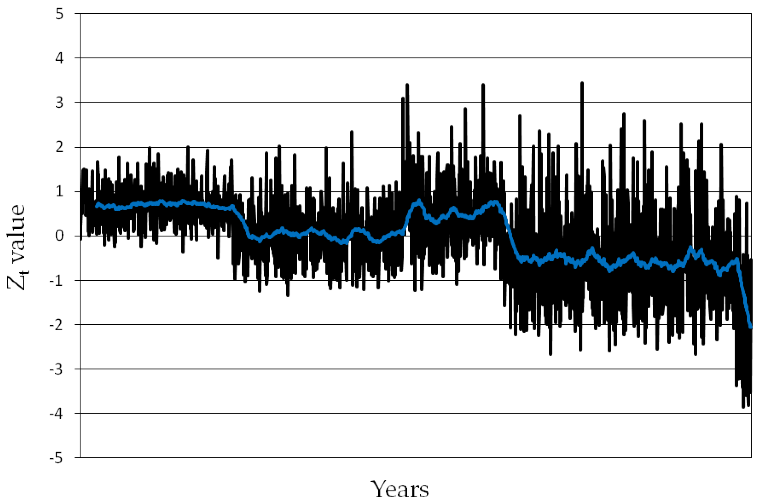
Figure 2.
Annual Zt values (black bars) calculated from observed Po River mean annual discharge from the 1918 to 2025 CE. The blue thick black line indicates the 10-year moving average. The horizontal lines at Z= -1, Z = -2 and Z= -3 denotes the threshold for moderate, severe and extreme deficits, respectively.
Figure 2.
Annual Zt values (black bars) calculated from observed Po River mean annual discharge from the 1918 to 2025 CE. The blue thick black line indicates the 10-year moving average. The horizontal lines at Z= -1, Z = -2 and Z= -3 denotes the threshold for moderate, severe and extreme deficits, respectively.
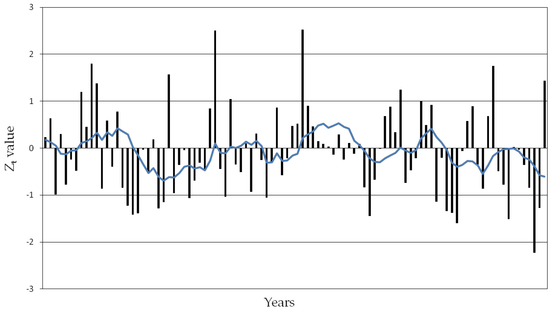

Table 1.
– Selected parameters (μi - mean flow rates for each period; σi - standard deviation of flow rates) for the six macro-climatic periods considered in this study along with corresponding references from which aforementioned parameters were derived. Coefficient of Variation (CV= σi /μi) for each climate period is also reported.
Table 1.
– Selected parameters (μi - mean flow rates for each period; σi - standard deviation of flow rates) for the six macro-climatic periods considered in this study along with corresponding references from which aforementioned parameters were derived. Coefficient of Variation (CV= σi /μi) for each climate period is also reported.
| Climate period | Years CE | Length (years) | μi | σi | Cv | Main characteristics | References | |
|---|---|---|---|---|---|---|---|---|
| Roman Period | 0-450 | 450 | 1.2 | 0.1 | 0.08 | warm climate with well-distributed precipitation | [12,13] | |
| Early Middle Ages | 450-950 | 500 | 1.05 | 0.15 | 0.14 | transitional dynamics with slight cooling and increased instability | [12,13] | |
| Medieval Period | 950-1250 | 300 | 1.15 | 0.18 | 0.16 | warm climate with well-distributed precipitation | [12,13] | |
| Little Ice Age | 1300-1850 | 550 | 0.90 | 0.25 | 0.28 | harsh climate with long, snowy winters, with variability linked to harsh winter cycles | [12,13] | |
| Modern Period | 1850-1980 | 130 | 0.85 | 0.20 | 0.24 | gradual return to mild temperatures and well-distributed precipitation | [14,15] | |
| Contemporary Period | 1980-2025 | 45 | 0.55 | 0.38 | 0.69 | high variability in snowfall, temperature and precipitation data | [14,15] |
Table 2.
– Spell analysis of reconstructed years with moderate deficit (Zt < -1), severe deficit (Zt < -2), extreme deficit (Zt < -3) and exceptional deficit (Zt < -4) in the Northern Apennines. The number of events with different rates of deficits were also added to the analysis along with the corresponding maximum length (in years).
Table 2.
– Spell analysis of reconstructed years with moderate deficit (Zt < -1), severe deficit (Zt < -2), extreme deficit (Zt < -3) and exceptional deficit (Zt < -4) in the Northern Apennines. The number of events with different rates of deficits were also added to the analysis along with the corresponding maximum length (in years).
| Climate period | Length (years) | Years with moderate deficit | Years with severe deficit | Years with extreme deficit | Years with exceptional deficit | N. of 2 continuous years with moderate or severe or extreme deficit | Maximum length (in years) of event with moderate or severe or extreme deficit |
|---|---|---|---|---|---|---|---|
| Roman Period | 450 | 0 | 0 | 0 | 0 | 0-0-0 | 0-0-0 |
| Early Middle Ages | 500 | 18 | 0 | 0 | 0 | 0-0-0 | 0-0-0 |
| Medieval Period | 300 | 3 | 0 | 0 | 0 | 0-0-0 | 0-0-0 |
| Little Ice Age | 550 | 195 | 26 | 0 | 0 | 47-1-0 | 5-2-0 |
| Modern Period | 130 | 52 | 3 | 0 | 0 | 13-0-0 | 9-2-0 |
| Contemporary Period | 45 | 34 | 25 | 10 | 0 | 6-5-4 | 8-3-2 |
Table 3.
– Sensitivity analysis testing the stability of moderate deficit (Zt < -1), severe deficit (Zt < -2), extreme deficit (Zt < -3) frequencies as well as spell occurrences in the Contemporary Period (1980-2025) under perturbed parameter scenarios.
Table 3.
– Sensitivity analysis testing the stability of moderate deficit (Zt < -1), severe deficit (Zt < -2), extreme deficit (Zt < -3) frequencies as well as spell occurrences in the Contemporary Period (1980-2025) under perturbed parameter scenarios.
| Scenario | Perturbation applied to the Contemporary Period | Years with moderate deficit | Years with severe deficit | Years with extreme deficit | N. of 2 continuous years with moderate or severe or extreme deficit | Maximum length (in years) with moderate or severe ore extreme deficit |
|---|---|---|---|---|---|---|
| Baseline | none | 34 | 25 | 10 | 6-5-4 | 8-3-2 |
| Convergence (conservative) | μ = + 5% σ = - 10% | 25 | 17 | 6 | 5-4-2 | 4-2-0 |
| Divergence (pessimistic) | μ = - 5% σ = + 10% | 37 | 28 | 13 | 8-6-4 | 8-5-3 |
Table 4.
– Spell analysis of the observed annual discharge data from the Po River (Pontelagoscuro gauge). The analysis compares the occurrence of moderate (Zt < -1) and severe (Zt < -2) deficits across the historical baseline and the contemporary period.
Table 4.
– Spell analysis of the observed annual discharge data from the Po River (Pontelagoscuro gauge). The analysis compares the occurrence of moderate (Zt < -1) and severe (Zt < -2) deficits across the historical baseline and the contemporary period.
| Period | Length (years) | Years with moderate deficit | Years with severe deficit | N. of 2 continuous years with moderate deficit | Maximum length (in years) with moderate deficit | Specific year with moderate deficit | Specific year with severe deficit |
|---|---|---|---|---|---|---|---|
| Historical Baseline | 62 | 9 | 0 | 2 | 3 | 1943-1945; 1949-1950; 1955; 1962; 1970 | - |
| Contemporary Period | 45 | 8 | 1 | 2 | 3 | 1990; 2003; 2005-2007; 2017; 2022-2023 | 2022 |
Disclaimer/Publisher’s Note: The statements, opinions and data contained in all publications are solely those of the individual author(s) and contributor(s) and not of MDPI and/or the editor(s). MDPI and/or the editor(s) disclaim responsibility for any injury to people or property resulting from any ideas, methods, instructions or products referred to in the content. |
© 2026 by the authors. Licensee MDPI, Basel, Switzerland. This article is an open access article distributed under the terms and conditions of the Creative Commons Attribution (CC BY) license (http://creativecommons.org/licenses/by/4.0/).
Copyright: This open access article is published under a Creative Commons CC BY 4.0 license, which permit the free download, distribution, and reuse, provided that the author and preprint are cited in any reuse.


