

Submitted:
30 June 2026
Posted:
01 July 2026
You are already at the latest version
Abstract
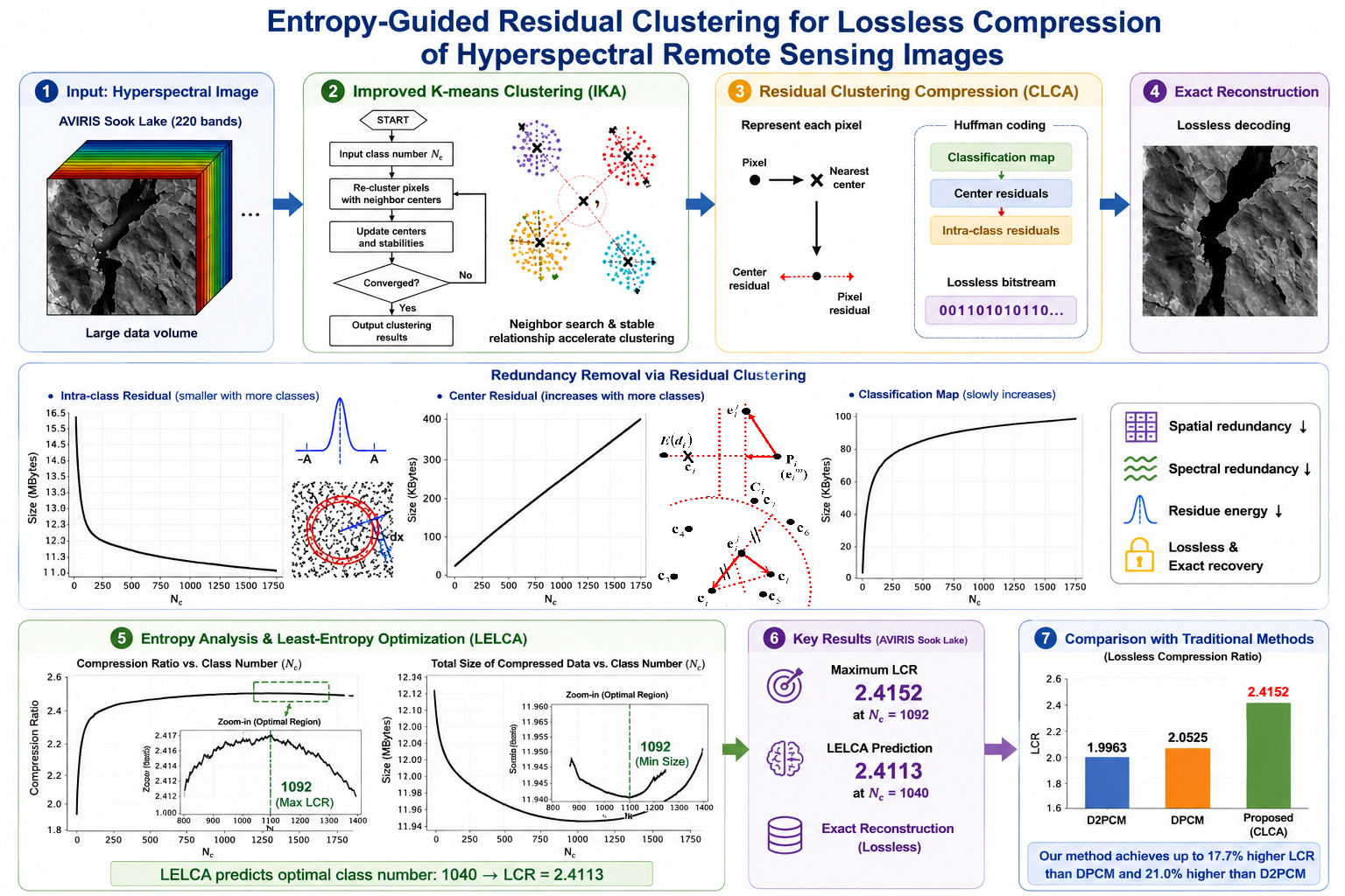
Hyperspectral remote sensing images contain abundant spectral information but generate extremely large datasets, creating significant challenges for storage and transmission. Lossless compression is essential in scientific remote sensing because it preserves the complete spectral information required for subsequent analysis. This study proposes a residual clustering-based lossless compression framework for remotely sensed images. An improved K-means algorithm (IKA) is developed to accelerate clustering by exploiting historical clustering results, preserving stable inter-class relationships, and restricting distance calculations to neighboring cluster centers. Based on the fast clustering mechanism, a clustering lossless compression algorithm (CLCA) is constructed to enhance intra-class redundancy and to encode class maps, clustering-center residuals, and pixel residuals using Huffman coding. Probability distribution models are further developed to analyze the entropy characteristics of the compression components, leading to a least-entropy lossless compression algorithm (LELCA) to predict the optimal number of clusters. Experiments were conducted using the 220-band AVIRIS Sook Lake hyperspectral dataset. The proposed CLCA achieved a maximum lossless compression ratio of 2.4152 with 1092 classes. LELCA predicted an optimal class number of 1040 with a compression ratio of 2.4113, demonstrating good agreement with exhaustive search results. Compared with conventional differential pulse-code modulation (DPCM) and second-order DPCM (D2PCM), which obtained compression ratios of 2.0525 and 1.9963, respectively, the proposed approach provided substantially higher compression efficiency. The results indicate that entropy-guided clustering effectively removes spatial and spectral redundancy while maintaining exact reconstruction. The proposed framework offers an efficient, theoretically grounded solution for lossless compression of hyperspectral remote sensing images. It provides a practical approach to determining the optimal clustering configuration without exhaustive parameter searches.
Keywords:
hyperspectral image
; lossless compression
; improved K-means clustering
; entropy analysis
; residual coding
; Huffman coding
; remote sensing
; AVIRIS
1. Introduction
Hyperspectral remote sensing has become an essential technology for observing, measuring, and interpreting complex physical, chemical, and biological phenomena on the Earth’s surface. Unlike conventional RGB imaging, which records only three broad visible channels, hyperspectral sensors acquire hundreds or even thousands of narrow and contiguous spectral bands, typically spanning wavelengths from approximately 400 nm to 2500 nm. This rich spectral representation enables the identification of subtle material properties that are difficult or impossible to distinguish in standard images. As a result, hyperspectral imagery has been widely used in surveillance [1], mineral exploration [2], industrial inspection [3], precision agriculture [4], and environmental monitoring [5]. However, the same spectral richness that makes hyperspectral data valuable also produces extremely large data volumes. Efficient compression is therefore necessary to reduce storage requirements, accelerate transmission, and support practical deployment in airborne, satellite, and field-based remote sensing systems.
Compression methods for hyperspectral imagery are generally classified into lossy, near-lossless, and lossless approaches. Lossy compression can achieve high compression ratios by discarding information deemed visually or statistically less important, but it is irreversible. Although lossy methods may suppress sensor noise, they may also remove weak but scientifically meaningful spectral features or introduce compression artifacts. Such distortions can reduce the reliability of subsequent analysis, especially when the data are used for classification, target detection, anomaly identification, or quantitative retrieval. Near-lossless methods seek a balance between compression efficiency and bounded reconstruction error and have been investigated through techniques such as the Karhunen–Loève transform [6], principal component analysis, vector quantization, and JPEG2000-based coding [7]. These methods can improve rate–distortion performance and computational efficiency, but they still do not guarantee exact recovery of the original data.
Lossless compression, by contrast, preserves the original image without any numerical alteration. Every pixel value and every spectral band can be reconstructed exactly after decompression. This property is particularly important for scientific remote sensing, where raw observations may need to be reanalyzed using future algorithms, validated against field measurements, or archived as reference data. Lossless preservation is also critical in domains such as medical hyperspectral imaging [8] and material characterization [9], where small spectral variations may carry diagnostic or structural significance. Although lossless compression usually yields lower compression ratios than lossy alternatives, its ability to maintain complete data integrity makes it indispensable for applications where information loss is unacceptable.
Traditional lossless image compression is built on several major principles: entropy coding, dictionary-based coding, predictive coding, and transform-based decorrelation. Classical methods such as run-length encoding, Huffman coding, arithmetic coding, Lempel–Ziv family algorithms, and prediction by partial matching have strongly influenced many widely used compression standards and file formats [10]. Dictionary-based approaches, including LZ77, LZ78, and LZW, have been adopted in practical systems such as ZIP, PNG, and GZIP because of their simplicity and efficiency [11]. Entropy coding methods remain important because they assign shorter codewords to frequently occurring symbols, thereby reducing the average number of bits required for representation. However, hyperspectral images introduce additional challenges because redundancy exists not only within spatial neighborhoods but also across adjacent spectral bands.
In remote sensing, several lossless compression algorithms have been developed specifically for multispectral and hyperspectral imagery, including clustering vector quantization, predictive trees [12], differential pulse-code modulation methods [13], and other spatial–spectral prediction schemes [14]. Arnavut et al. [15] proposed a method in which one band is compressed using lossless JPEG. In contrast, subsequent bands are reordered based on the sorting permutation of previous bands and then encoded using move-to-front coding to reduce entropy. The CCSDS 123.0-B standard [16] is among the most widely recognized real-time lossless hyperspectral compression standards. It operates by first generating predictions of incoming samples and then encoding the differences between predicted and actual values. This approach has been reported to achieve compression ratios of approximately 50–60%. Álvarez-Cortés et al. [17,18] combined Regression Wavelet Analysis with the CCSDS-123.0-B-1 predictor and a lightweight contextual arithmetic coder, achieving notable coding gains over RWA combined with JPEG2000 [19]. Other studies have shown that integral wavelet transforms [20] and clustering-based methods can effectively reduce both spatial and structural redundancies, thereby improving the compression of multispectral images [21].
Predictive coding has become one of the most influential strategies for lossless hyperspectral image compression. In this approach, a pixel or spectral sample is estimated from previously encoded neighboring samples, and only the prediction residual is encoded. Since residuals usually have lower entropy than the original data, they can be represented more compactly. Context-dependent predictors further improve this process by adapting the prediction model to local image characteristics. Ulacha and Łazoryszczak [22] proposed a context-dependent linear prediction method based on mean absolute error minimization and reported better compression performance than conventional predictors. Rajput et al. [23] introduced content-aware prediction mechanisms that dynamically adjust to image characteristics, making predictive compression more suitable for efficient data sharing and distributed storage environments.
More recently, machine learning has opened new directions for lossless compression. Instead of relying solely on manually designed predictors or fixed statistical models, neural-network-based methods can learn complex dependencies directly from training data. Rhee et al. [24] proposed a duplex neural network architecture that predicts both pixel values and contextual information for lossless image compression, achieving performance improvements over traditional methods. Sun et al. [25,26] further surveyed and benchmarked neural universal compressors, showing that deep learning models are increasingly competitive for compressing diverse data sources. These approaches suggest a broader transition from conventional statistical compression toward adaptive and intelligent compression systems.
For hyperspectral and multispectral remote sensing data, compression performance depends heavily on how effectively spatial, spectral, and structural redundancies are removed. Recent studies have therefore focused on spectral decorrelation, predictive modeling, transform coding, and hybrid compression frameworks. Altamimi and Ben Youssef [27] reviewed lossless and near-lossless hyperspectral compression techniques and emphasized the importance of maintaining spectral fidelity. Nagendran et al. [28] proposed a lossless framework that combines spectral decorrelation with transform coding to reduce inter-band redundancy. These studies demonstrate that exploiting the strong correlation among neighboring spectral bands is essential for improving compression efficiency without sacrificing reconstruction accuracy.
The entropy-based lossless compression algorithms are based on the improved K-means algorithm (IKA), which efficiently improves the K-means clustering algorithm [21] by accounting for the spatial geometric relationships among remotely sensed pixels. The best class number can be predicted from entropy analysis of the probability distribution models for the clustering lossless compression algorithm (CLCA). The predicted best class number closely matches the experimental results, where the class number sweeps from 1 to a large value to locate the class number that has the highest lossless compression ratio (LCR).
This article is a revised and expanded version of a paper entitled “Entropy Analysis for Clustering Based Lossless Compression of Remotely Sensed Images” [29], which was presented virtually at 2021 IEEE Big Data Conference on Dec. 18, 2021.
2. Methods
2.1. Improve K-Means Algorithm (IKA)
In the K-means algorithm [21], every pixel calculates the Euclidean distance with all clustering centers to determine its assignment, so clustering a large number of classes is a relatively time-consuming task. Actually, classes far from the pixel do not need to be analyzed, and stable classes do not need re-clustering. To create one more class, the class with the most irregular spatial distribution or the largest standard deviation can be divided according to its spreading direction. These strategies can help the clustering converge faster.
In the improved K-means algorithm (IKA) (shown in Figure 1), it is supposed that Ns is the total number of pixels attending clustering; b is the number of bands; nc is the number of classes; Ci is the set of pixels in the class i; N(Ci) is the number of pixels in class i; ci is the center of class i; cil is the value of lth band for ci; cilastl is the lth band value of ci in the previous iteration; eijis the jth pixel in class i (eij∈Ci); eijl is the value of lth band for pixel eij; Cij is the set of classes that need to make re-clustering judgment with pixel eij; dij is the distance between pixel eij∈Ci and clustering center ci; dij is the distance from class i to class j; dijk is the distance from the pixel eijto the center of class k; array Pd[i] =max({dij|eij∈Ci}) (i∈[0,nc]) is a collection of the maximum deviate distances for the nc classes, and Pi={eim |dim=max({dij|eij∈Ci})) corresponds to the pixel eim with the maximum of dij in the class i; E(di) is the mean of {dij|eij∈Ci}; lastsign[i], used to judge inter-class stability, is the modification mark of class i in the previous iteration; sign[i], used to judge clustering convergence, is the modification mark of class i in the current iteration; εc is the maximal iterative error of clustering centers.
- 1
- Nc initial clustering centers ci (i∈[0, Nc-1]) are created according to the initial spatial division.
- (a)
- If the previous clustering record with the class number Nc′ exists, the previous clustering environment, including class centers, pixel status, and other important information, is rebuilt, setting nc=Nc′. Otherwise, all pixels are grouped into a single class C0, with nc=1, meaning the one-class space has Ns pixels. The clustering center c0 is calculated as (1) with i=0, and the initial clustering status, lastsign, is assigned with lastsign [0]=1. The distances d0j(j∈[0, Ns-1]) (from (2) with i=0) between the intra-class pixels e0jand their center c0 are sorted in descending order, and the maximal value of d0j(j∈[0, Ns-1]) is saved to Pd [0] corresponding to the farthest pixel P0 to the center c0.
- (b)
- The pixel eim in the class Ci that is the farthest from the center ci is noted as Pi, and this maximal distance for class i is recorded in Pd[i] (i∈ [ 0, nc-1]). Along the direction = ci -eim in (3), this class is divided according to the vertical plane passing through the middle point between the farthest pixel eim and the point that has a distance of E(di) with ci along the inverse direction of , creating two new classes Cnc and Ci′ as (4) (see Figure 2a). Ci′ will take the place of Ci, letting Ci=Ci′. Their sizes are N(Cnc) and N(Ci), respectively. The two new classes are updated, including the following values: for an instance of the new class Ci, the class center ci (1), the distance dij between the intra-class pixel eij ∈ Ci and its center (2), E(di), Pd[i], and Pi.
Let lastsign[i]=lastsign[nc]=1 and nc=nc+1. When the number of classes is reached, i.e., nc==Nc, terminate the class division stage and proceed to step 2; otherwise, proceed to step 1b and continue the division process.
- 2.
- The clustering centers before division or in the previous iteration are recorded in cilast, letting cilast =ci (i∈[0, Nc - 1]), and the class modification mark in the current iteration, sign, is set as sign[i]=0 (i∈[0, Nc-1]).
- 3.
- The distance matrix D={dij, i,j∈[0, Nc - 1]} is created by calculating the Euclidean distance as (5) between any two class centers.
- 4.
- For each pixel eij∈Ciin class i∈[0, Nc - 1], dij(j≠i, j∈[0, Nc - 1]) are sorted in ascending sequence to create one array Cij (for k∈Cij, exists k≠i, k∈[0, Nc - 1], dij>0.5dik), defining the search order for pixel eij, where the class with smaller distance to the class i is in the preceding position (see Figure 2b). The class centers with a distance to the class center ci larger than 2dij are not under consideration.
- 5.
- For each neighbor class k in Cij, if lastsign[i]==0 and lastsign[k]==0 (k∈Cij), meaning the relationship between classes j and k is stable, k is removed from Cij because it is not necessary to make Euclidean analysis between them. Otherwise, the pixel eij must be re-clustered: the distance dijk between eij and the center ck is calculated. For the class l≠i with the minimal value {l|dijl=min{{dijk|k∈Cij},dij}} (6), pixel eij is combined with the class l whose center is nearest to it, modifying class sets: Ci=Ci-{eij}, Cl=Cl+{eij}, and setting the class modification marks as sign[i]=1 and sign[l]=1.
- 6.
- For each class i∈[0, Nc-1] whose sign[i]==1, ci and dij (eij∈Ci) are updated according to (5) and (6). If |clilast-cli|< εc (l∈[1, b]), class i is assumed stable, setting sign[i]=0.
- 7.
- If none of the classes are changed, sign[i]==0 (i∈[0, Nc-1]), or the iteration number reaches the limit, the clustering process ends and proceeds to step 8; otherwise, it proceeds to step 2.
- 8.
- The previous clustering status lastsign is updated to lastsign=sign to record class stability in the current iteration.
- 9.
- Current clustering results are saved, including the class structure and all the variables.
Initial clustering continues working on the previous clustering results and divides the class with the maximum deviation value in P[]. This way not only saves initial clustering time but also preserves the stable relationships between classes formed by the clustering process.
In this algorithm, only classes whose correlations show changes will be re-clustered; intra-class pixels merely compute distances to neighboring class centers. So, during the iterative process, the statuses of more classes are stable, leading to higher clustering velocity.
2.2. Process of Clustering Lossless Compression Algorithm
Based on the fast IKA clustering for high class numbers, the clustering lossless compression algorithm (CLCA) could ultimately reduce intra-class redundancy. However, statistical Huffman coding could utilize this redundancy to improve the lossless compression ratio (LCA). Since the relationship between neighboring bands is strongest, clustering centers could eliminate spectral redundancy between them.
Supposed that m, n, b are respectively the length, width, and band number of remotely sensed images, Xj, ki is the kth band data of the jth sample in the ith class, Iki is the kth band data of the ith class center, N(i) is pixel number of the ith class, sij is the class serial number of pixel (i, j) (spatial coordinates). Then the detailed process of CLCA is provided as follows:
- 1
- For remotely sensed images, apply IKA clustering, creating Nc class centers Ii, i∈[0, Nc-1] (choose the intra-class pixel nearest to the original computed clustering center as the center of this class, this has less error compared with directly being rounded to integer), and classification map S={sij∈[0, Nc - 1],i∈[0, m-1],j∈[0, n-1]}. And apply statistical Huffman coding to S at the same time.
- 2
- Code clustering centers:
- (a)
- Compute spectral residue of each center:
- (b)
- Compute the residue of the first band data between all classes:
- (c)
- Apply Huffman statistical coding to the residue data , and is saved separately.
- 3.
- Code intra-class pixels:
- (a)
- Compute residue between each intra-class pixel and its center:
- (b)
- Apply statistical Huffman coding to the residue
The preceding two steps of this algorithm, 1) and 2), could realize VQ compression, whose compression ratio (CR) could reach hundreds of times. Using the preceding clustering results, we could quickly determine CR for different class numbers to identify the best class number.
2.3. Probability Model Analysis of CLCA
Assuming that the number of pixels is Ns and the number of classes is Nc, the probability distribution model of the residue data for CLCA is analyzed as follows.
- Intra-class residue:
When the number of classes reaches a pre-defined value Nc, the intra-class residue is a set X={0, ±1, ±2, …}, the element of which is a variable x∈X approximately taking on a Gaussian distribution . Maximum entropy with a limited mean and variance is provided in (10) [6].
Then, the total number of bits for the intra-class residue is given by (11).
- 2.
- Class center residue:
Supposed that A=(fmax - fmin) (fmax and fmin respectively represent the maximal and minimal values of all bands for all class centers), if the number of bands is high enough, the class center residue data x∈[-A, A] approximately take on a Gauss distribution (Figure 3a), whose maximum entropy with a limited mean and deviance is (12).
Then the total number of bits for the class center residue is (13).
- 3.
- Classification map:
The classification map data X={0, 1, 2, …, Nc} take on a uniform distribution with probability density function p3(x)=1/Nc, whose entropy is H3=log2Nc, so the total number of coded bits is
B3=NsH3=Nslog2Nc
- 4.
- The total number of bits in CLCA is given by (14).
B3 has a logarithmic relationship with the number of classes Nc, so the change of Nc has little influence on B3. When the class number Nc is small, σ1 changes noticeably, decreasing as Nc increases. So, B depends on B1 and decreases as Nc increases. When the class number Nc is high enough, B increases linearly with the increase in Nc.
2.4. Least Entropy Lossless Compression Algorithm
The Least Entropy Lossless Compression Algorithm (LELCA) calculates the class number with the fewest compression bits for CLCA. Suppose that if Nc increases m times, (Nc, σ1) turns into (Nc′, σ1′) described in equations (16), where k and x are to be determined.
From (16), the class number Nc and the intra-class pixel standard deviation σ1 are related as described in Equation (17).
Equation (17) can also be expressed as Equation (18).
Nc can be derived as Equation (19).
There are three unknown parameters, x, k, and k2, which can be calculated using three initial conditions, as described by Equation (20).
Solving the equations (20), we have equations (21) and (22).
and,
Then we can derive Equation (23).
We can set dB/dNc = 0 to obtain the optimal class number that yields the highest compression ratio. From Equation (15),
The best number of classes can be predicted by Equation (24), where σ2 is the standard deviation of clustering centers’ residue.
The LELCA algorithm is proposed as follows based on Equation (24) to obtain the best class number and the corresponding best LCR.
- Choose initial three class numbers: n1, n2, n3.
- Cluster the space into n1 classes and use CLCA to get σ1n1, σ2n1, and Huffman coding length L1; cluster the space into n2 classes and use CLCA to get σ1n2, σ2n2, and Huffman coding length L2; cluster the space into n3 classes and use CLCA to get σ1n3, σ2n3, and Huffman coding length L3.
- According to the prediction Equation (24), assuming σ1 = σ1n3 and σ2 = σ2n3, Ncbest is calculated. If Ncbest is in the list of the initial and predicted class numbers, go to step 7 to terminate.
- Cluster the space into Ncbest classes and use CLCA to get its corresponding σ1best, σ2best, and code length Lbest.
- Update n1, n2, n3: (1) sort all the initial and predicted class numbers from low value to high value as an array; (2) search the array from left to right; the class number with the lowest code length is set as n3; (3) the previous two class numbers on the left in the array are set as n1 and n2.
- Go to step 2.
- In the list of the initial and predicted class numbers, class number n with the smallest Huffman coding length L is the best.
2.5. Conditions of Ultimate Division of Classes
When continuing dividing the intra-class pixels which shows a Gaussian distribution when class number is small, more intra-class pixels take on a spatially uniform distribution (see Figure 3b), noting that intra-class residue x∈[0, R] does not take on a uniform distribution). According to the Equation (54) in Appendix A, in b-dimensional space Vb, the probability distribution is p1(x) in (25), with entropy H1 in (26).
If R≈σ1, H1 is similar in form to the H1 in (10). When the class number reaches Nc0 (here, σ1=σ10), if σ1 is reduced m times, then σ1′=σ1/m, Nc0′=mbNc0. The class number Nc and the standard deviation of intra-class pixels have the relation of Equation (27).
The (27) can be further expressed as (28) along with an initial condition.
Then
According to initial condition, (29) can be rewritten as
Then
Then
which is a constant. Then
Here, total entropy B is determined by B2. When one class is added, B increases by (bits).
3. Results
Sook Lake 220-band AVIRIS images (256×256, 16-bit, obtained from [29], Figure 4a) were selected for algorithm analysis. The lossless compression ratio (LCR) is defined as (34).
3.1. IKA
In the IKA clustering algorithm, with εc=0.01 and Nc=100, it converges after 214 iterations; LCR is 2.3075, and the average iteration time is 8 seconds. Figure 4b is the gray balanced result of the rebuilt 60th band image using the IKA clustering results of 100 class centers, where the intra-class pixels are present uniformly using their class center. This is a near-lossless compression method.
Suppose Nc=200. Then the initial clustering further divides the space based on the clustering results of Nc=100, taking only 3s, converging after 210 iterations. Each iteration takes an average of 9s, and LCR reaches 2.3607. So, an increased class number has little influence on clustering iteration speed; however, traditional K-means needs 6 minutes (100 classes) for one iteration, and clustering time increases abruptly with the increased class number.
3.2. CLCA
The clustering a class number makes full use of historical clustering results, enabling lossless compression of each class number at high velocity. Figure 5, Figure 6, Figure 7, Figure 8 and Figure 9 shows the clustering results for class numbers from 1 to 1780, with a maximum of 20 iterations, and εc is set to 0.02. Figure 5 shows that intra-class residue B1 has an inverse tendency to the class number, because σ1 decreases with the increase of class number. The more classes in space, the smaller the occupied area of a class. Therefore, Figure 5 meets the supposition of the probability model in Equation (11).
In Figure 6, the clustering centers’ residue B2 shows an approximately linear relationship with Nc, consistent with the assumptions of the probability model in Equation (13).
In Figure 7, the classification map coding B3 has a logarithmic relationship with the number of classes, Nc, as given by the Equation (14), so when Nc is a large number, the change of Nc has little influence on B3.
When the number of classes Nc increases, σ1 and B1 decrease (Figure 5), but B2 and B3 increase (Figure 6 and Figure 7). From Figure 8, the total length of the code and codebook reaches a minimum at Nc=1092, where the LCR reaches a maximum of 2.4152 (Figure 9). When the class number is less than 1092, the reduced amount of B1 is larger than the increased amount of B2+B3, leading to an increased LCR; when the class number is higher than 1092, the reduced amount of B1 is less than the increased amount of B2+B3.
3.3. Estimation of the Best Compression of CLCA
The least-entropy lossless compression algorithm (LELCA) is used to estimate the optimal class number Nc that yields the best compression with CLCA. In Table 1, the left table shows the clustering results for different class numbers, from the input and the predicted Ncbest using (24); the right table shows the execution of LELCA, where the number of iterations for clustering a class number has no limit, and εc is set to 0.0001. The execution process for LELCA is provided below and in Table 1.
- Setting n1=200, n2=300, n3=400 as input parameters, their σ1n1=35.407818, σ1n2=33.676117, and σ1n1=32.581664. According to Equation (24), Ncbest=1023, whose σ1= 29.458689, σ2 =232.382148, Lbest=11959639 and LCR is 2.411096.
- Updating n1=300, n2=400, n3=1023, according to Equation (24), Ncbest=934, whose σ1= 29.763009, σ2 =233.284102, Lbest=11966192 and LCR is 2.409776.
- Updating n1=400, n2=934, n3=1023, according to Equation (24), Ncbest=1040, whose σ1= 29.402593, σ2 =232.143746, Lbest=11958672 and LCR is 2.411291.
- Updating n1=934, n2=1023, n3=1040, according to Equation (24), Ncbest=1064, whose σ1= 29.360868, σ2 =231.907104, Lbest=11962256 and LCR is 2.410569.
- Updating n1=934, n2=1023, n3=1040, according to Equation (24), Ncbest=1064, which has been clustered in step 4. The LELCA converges and stops the iteration.
Therefore, the predicted best class number is 1040, with an LCR of 2.411291. The predicted best class number, 1040, is different from the best class number, 1092, obtained from sweeping the range of class numbers (Figure 8 and Figure 9). The reasons include (1) the prediction only considers σ1 and σ2 for calculating Ncbest, (2) the maximal iteration number in CLCA introduces noise in the sweep analysis of the range of class numbers. More information from the code length will enhance the accuracy of LELCA.
The iteration number decreases with the increased class numbers until reaching the best class number, 1040, whose iteration number is only 35; while the iteration number for the class number 200 is 199. When the class number is higher than the best class number, 1040, the iteration number increases.
3.4. Comparison with DPCM/D2PCM Algorithms
Two lossless compression algorithms, CLCA and DPCM, have a coding discrepancy of ΔB (equation 35), where B’ is from (58) in the Appendix B and B is from (15). Under normal conditions, σ1<σ1′, i.e., ΔB>0; when the number of bands b is extremely high, likely, σ1>σ1′, but current remote sensing equipment cannot meet this requirement. So, the CLCA algorithm is more efficient than the DPCM algorithm.
When using DPCM, σ1′=177, B′=14,048,912 bytes, and the lossless compression ratio is 2.0525, so CLCA is more efficient than DPCM. However, for D2PCM, σ1′ is 190.957, and LCR is 1.9963. Therefore, spectral second-order residue cannot increase LCR. Table 2 shows that LELCA yields the best class number and highest LCR but is more time-consuming because it uses an iterative method to determine the optimal class number.
5. Discussion
The experimental results demonstrate that entropy-guided clustering provides an effective mechanism for removing both spectral and spatial redundancy in hyperspectral images while maintaining exact reconstruction. Unlike conventional predictive coding approaches, the proposed framework exploits pixel similarities via clustering and represents both class centers and intra-class deviations using residual coding. This strategy transforms highly correlated hyperspectral data into lower-entropy representations that can be efficiently encoded using Huffman coding. The results obtained from the AVIRIS Sook Lake dataset indicate that clustering-based residual representation provides a practical alternative to traditional predictive lossless compression techniques.
The improved K-means algorithm (IKA) plays a crucial role in enabling efficient clustering with a large number of classes. Conventional K-means requires distance calculations between each pixel and all cluster centers, leading to rapidly increasing computational complexity as the number of clusters grows. By leveraging prior clustering results, preserving stable inter-class relationships, and restricting pixel reassignment to neighboring classes, the proposed IKA substantially reduces unnecessary computations while maintaining convergence speed, even for large class counts. The results for 100- and 200-class problems demonstrate that increasing the number of clusters does not significantly increase the iteration time, making the algorithm suitable for high-dimensional hyperspectral datasets.
The experimentally observed behavior of the compression components agrees well with the theoretical probability models derived in Section 2. As the number of classes increases, the intra-class standard deviation decreases, resulting in a reduction of the intra-class residual coding length. At the same time, the coding lengths associated with class-center residuals and classification maps increase. These opposing trends explain the existence of an optimal class number. The minimum total coding length observed near 1092 classes confirms the entropy analysis and validates the assumptions underlying the CLCA probability model. Therefore, the proposed entropy framework provides not only a compression method but also a theoretical explanation of the relationship between the number of clusters and coding efficiency.
The least-entropy lossless compression algorithm (LELCA) further demonstrates that exhaustive searches over all class numbers are unnecessary. Based on the entropy model and a limited number of initial clustering results, LELCA predicted an optimal class number of 1040 and achieved a compression ratio of 2.4113, which is very close to the maximum compression ratio of 2.4152 obtained by exhaustive analysis. The small discrepancy between the predicted and experimental optimum can be attributed to simplifying assumptions in the entropy model and the limited number of iterations used during sweeping analysis. Nevertheless, the prediction accuracy indicates that entropy-based parameter estimation provides a practical means of determining near-optimal clustering configurations with significantly reduced computational cost.
Compared with DPCM and D2PCM, the proposed clustering-based framework achieved noticeably higher compression ratios. DPCM and D2PCM primarily exploit spectral correlations between neighboring bands, whereas CLCA simultaneously utilizes spatial and spectral redundancy through clustering and residual coding. Experimental results show that DPCM achieved a lossless compression ratio of 2.0525, D2PCM obtained 1.9963, and the proposed method achieved compression ratios exceeding 2.41. These results suggest that clustering-based residual representation is more effective than first- and second-order spectral differencing for the AVIRIS dataset considered in this study. Furthermore, the degradation observed in D2PCM indicates that higher-order spectral differencing does not necessarily improve compression performance, as it may increase entropy rather than reduce it.
Although the proposed approach provides improved compression performance, several limitations should be noted. First, the entropy model assumes approximately Gaussian distributions for residual data, which may not accurately describe all remotely sensed images. Second, Huffman coding is used as the entropy coder; more sophisticated coders, such as arithmetic coding or context-adaptive coding, may provide additional coding gains. Third, the experimental evaluation was performed on a single AVIRIS dataset, and broader validation using images from different sensors and resolutions would strengthen the generality of the conclusions. In addition, the computational complexity associated with clustering large-scale hyperspectral datasets may become significant for onboard or real-time applications.
Overall, the results demonstrate that residual clustering and entropy analysis provide a unified framework for lossless hyperspectral image compression. The agreement between theoretical predictions and experimental observations confirms the validity of the proposed probability models and the effectiveness of entropy-guided cluster optimization. Future research may focus on adaptive clustering strategies, context-based entropy coding, parallel implementations, and machine-learning-assisted prediction models. Combining entropy-guided clustering with deep neural compression techniques may further improve compression efficiency and enable practical deployment in next-generation hyperspectral remote sensing systems.
6. Conclusions
Hyperspectral remote sensing images contain substantial spatial and spectral redundancy, making efficient lossless compression essential for long-term storage, transmission, and scientific analysis. This study presented a residual clustering-based lossless compression framework that combines an improved K-means clustering algorithm (IKA), a clustering-based lossless compression algorithm (CLCA), and a least-entropy lossless compression algorithm (LELCA) to determine the optimal number of clusters. By exploiting prior clustering results, preserving stable inter-class relationships, and limiting distance calculations to neighboring classes, the proposed IKA significantly accelerates convergence and enables efficient clustering for large numbers of classes.
Based on the clustering results, CLCA enhances intra-class redundancy and removes spectral correlation through residual coding and Huffman entropy coding. Probability distribution models were developed for the intra-class residuals, class-center residuals, and classification map, providing theoretical insight into the relationship between entropy and the number of clusters. Building on these models, LELCA predicts the class number that minimizes the total coding length without requiring exhaustive searches.
Experiments using the 220-band AVIRIS Sook Lake hyperspectral dataset demonstrated that the proposed approach effectively balances compression efficiency and computational complexity. The maximum lossless compression ratio obtained by CLCA was 2.4152 at 1092 classes, while LELCA predicted an optimal class number of 1040 and achieved a compression ratio of 2.4113, showing close agreement with exhaustive analysis. Compared with DPCM and D2PCM, whose compression ratios were 2.0525 and 1.9963, respectively, the proposed clustering-based method provided superior compression performance while preserving exact reconstruction of the original data.
The results indicate that entropy-guided clustering is an effective mechanism for reducing spatial and spectral redundancy in hyperspectral images. In addition to improving compression efficiency, the proposed framework provides a practical means of estimating optimal clustering parameters from entropy characteristics. Future work will investigate adaptive clustering strategies, more advanced entropy coders such as arithmetic coding and context-based coding, and deep-learning-assisted prediction models to improve compression efficiency further and extend the framework to larger hyperspectral datasets and real-time onboard remote sensing applications.
Funding
This research received funding support from the 2025 Yale University ASCEND Initiative and the 2025 NASA MPLAN.
Institutional Review Board Statement
Not applicable.
Informed Consent Statement
Not applicable.
Data Availability Statement
The original contributions presented in this study are included in the article. Further inquiries can be directed to the corresponding author.
Conflicts of Interest
The authors declare no conflicts of interest.
Appendix A
Appendix A.1. The Density Function of Equally Distributed Space
Pixel is
- 2D space
For an equally distributed two-dimensional circular space with maximal radius R at pixel density (Figure 3b), for the annulus between radius and , the pixel number is . The total number of pixels in that circular field is . Then we have one Equation (36).
Or
As dx is very small, we can assume (38).
So, the number of pixels at position x is , and the density function is given by (39).
- 2.
- 3D space
For an equally distributed sphere space with maximal radius R at pixel density (Figure 3b), for the annulus between radius and , the pixel number is . The total number of pixels in that circular field is . Then we have Equation (40).
Or,
As dx is very small, we can assume (38).
So, the number of pixels at position x is , and the density function is (43).
- 3.
- The n-dimensional Space
Following the same method, the density function in n-dimensional space is given by (44).
Assume that in n-dimensional space, there are n independent variables, x1, …, xn, described by (45) and (46).
We can get (47).
Then we can get the volume in (48).
where
For an equally distributed n-sphere space with maximal radius R and pixel density , in the annulus between radius and , the pixel number is (50).
According to (48), the total number of pixels in that circular field is . Then we have Equation (51).
Or,
As dx is very small, we can assume (53).
So, the pixel number at position x is , and the density function is (54).
Appendix A.2. Probability Distribution Model of DPCM/D2PCM Algorithms
According to [4], the detailed process of the DPCM lossless compression algorithm for hyperspectral images is as follows.
- Calculate spectral residue of each pixel according to (55).
- 2.
- Apply S+P integral wavelet transform [30] to the 1st band data, deleting spatial redundancy.
- 3.
- Apply Huffman statistical coding to residue dIk (k∈[1, b-1]) and solely save I(0,0).
D2PCM calculates the second-time residue of spectral data and makes amendments to the preceding steps: step 1 is added by , and in step 3, the residue is updated as dI1, d2Ik (k∈[2, b-1]).
The probability distribution model for DPCM/D2PCM can be derived as follows.
- 1.
- 2.
- The 1st band residue isX={0, ±1, ±2, …}; the variable x∈Xtakes on a Gaussian distribution N(0, σ2′2); then the total number of bits for the intra-class pixels’ residue is (57).
- 3.
- The total bit number of DPCM/ D2PCM algorithm is (58).
References
- Yuen, P.W.; Richardson, M. An introduction to hyperspectral imaging and its application for security, surveillance and target acquisition. Imaging Sci. J. 2010, 58, 241–253. [Google Scholar] [CrossRef]
- Fox, N.; Parbhakar-Fox, A.; Moltzen, J.; Feig, S.; Goemann, K.; Huntington, J. Applications of hyperspectral mineralogy for geoenvironmental characterization. Miner. Eng. 2017, 107, 63–77. [Google Scholar]
- Willoughby, C.T.; Folkman, M.A.; Figueroa, M.A. Application of hyperspectral-imaging spectrometer systems to industrial inspection. In Proceedings of the Three-Dimensional and Unconventional Imaging for Industrial Inspection and Metrology, Philadelphia, PA, USA, 19 January 1996; International Society for Optics and Photonics; Volume 2599, pp. 264–272. [Google Scholar]
- Park, B.; Lu, R. Hyperspectral Imaging Technology in Food and Agriculture; Springer: Berlin/Heidelberg, Germany, 2015. [Google Scholar]
- Obermeier, W.A.; Lehnert, L.W.; Pohl, M.J.; Gianonni, S.M.; Silva, B.; Seibert, R.; Bendix, J. Grassland ecosystem services in a changing environment: The potential of hyperspectral monitoring. Remote Sens. Environ. 2019, 232, 111273. [Google Scholar] [CrossRef]
- Wiegand, T.; Schwarz, H. Source coding: Part I of fundamentals of source and video coding. Found. Trends Signal Process. 2011, 4(1–2), 1–222. [Google Scholar] [CrossRef]
- Báscones, D.; González, C.; Mozos, D. Hyperspectral image compression using vector quantization, PCA and JPEG2000. Remote Sens. 2018, 10(6), 907. [Google Scholar] [CrossRef]
- Fei, B. Chapter 3.6—Hyperspectral imaging in medical applications. In Hyperspectral Imaging;Data Handling in Science and Technology; Amigo, J.M., Ed.; Elsevier: Amsterdam, The Netherlands, 2019; Volume 32, pp. 523–565. [Google Scholar]
- Selci, S. The future of hyperspectral imaging. J. Imaging 2019, 5, 84. [Google Scholar] [CrossRef] [PubMed]
- Hussain, A. J.; Al-Fayadh, A.; Radi, N. Image compression techniques: A survey in lossless and lossy algorithms. Neurocomputing 2018, vol. 300, 44–69. [Google Scholar] [CrossRef]
- Rahman, M. A.; Hamada, M. Lossless Image Compression Techniques: A State-of-the-Art Survey. Symmetry 2019, vol. 11(no. 10), 1274. [Google Scholar] [CrossRef]
- Mielikainen, J.; Toivanen, P. Clustered DPCM for the lossless compression of hyperspectral images. IEEE Trans. Geosci. Remote Sens. 2003, 41(12), 2943–2946. [Google Scholar] [CrossRef]
- Wang, J. F.; Zhang, K.; Tang, S. Spectral and spatial decorrelation of Landsat-TM data for lossless compression. IEEE Trans. Geosci. Remote Sens. 1995, 33(5), 1277–1285. [Google Scholar]
- Arnavut, Z.; Narumalani, S. Application of permutations to lossless compression of multispectral thematic mapper images. Opt. Eng. 1996, 35(12), 3442–3448. [Google Scholar] [CrossRef]
- Báscones, D.; González, C.; Mozos, D. FPGA Implementation of the CCSDS 1.2. 3 Standard for Real-Time Hyperspectral Lossless Compression. IEEE J. Sel. Top. Appl. Earth Obs. Remote Sens. 2018, 11(4), 1158–1165. [Google Scholar]
- Amrani, N.; Serra-Sagristà, J.; Laparra, V.; Marcellin, M. W.; Malo, J. Regression wavelet analysis for lossless coding of remote-sensing data. IEEE Trans. Geosci. Remote Sens. 2016, 54(9), 5616–5627. [Google Scholar] [CrossRef]
- Álvarez-Cortés, S.; Bartrina-Rapesta, J.; Serra-Sagristà, J. Multilevel split regression wavelet analysis for lossless compression of remote sensing data. IEEE Geosci. Remote Sens. Lett. 2018, 15(10), 1540–1544. [Google Scholar] [CrossRef]
- Swelends, W. The Lifting Scheme: A custom-design construction of biorthogonal wavelet. J. Appl. Comput. Harmon. Anal. 1996, 3(2), 186–220. [Google Scholar] [CrossRef]
- ISO/IEC 15444-1; Information Technology—JPEG 2000 Image Coding System—Part 1: Core Coding System. International Organization for Standardization: Geneva, Switzerland, 2000.
- Zhang, R.; Liu, Z.; Yu, N. Decorrelation of multispectral images for lossless compression. Proc. SPIE 2001, 4551, 215–219. [Google Scholar] [CrossRef]
- Theodoridis, S.; Koutroumba, K. Pattern Recognition; Academic Press: Cambridge, MA, 2008. [Google Scholar]
- Ulacha, G.; Łazoryszczak, M. Lossless Image Compression Using Context-Dependent Linear Prediction Based on Mean Absolute Error Minimization. Entropy 2024, 26(12), 1115. [Google Scholar] [CrossRef] [PubMed]
- Rajput, A.; Li, J.; Akhtar, F.; Khand, Z. H.; Hung, J. C.; Pei, Y.; Börner, A. A Content Awareness Module for Predictive Lossless Image Compression to Achieve High Throughput Data Sharing over Network Storage. Int. J. Distrib. Sens. Netw. 2022, 18(4). [Google Scholar] [CrossRef]
- Rhee, H.; Jang, Y. I.; Kim, S.; Cho, N. I. Lossless Image Compression by Joint Prediction of Pixel and Context Using Duplex Neural Networks. IEEE Access 2021, 9, 118830–118841. [Google Scholar] [CrossRef]
- Sun; Ma, H.; Ling, F.; Xie, H.; Sun, Y.; Yi, L. A survey and benchmark evaluation for neural-network-based lossless universal compressors toward multi-source data. Front. Comput. Sci. 2025, 19, 197360. [Google Scholar] [CrossRef]
- Memon, N. D.; Sayood, K.; Magliveras, S. S. Lossless compression of multispectral image data. IEEE Trans. Geosci. Remote Sens. 1994, 32(2), 282–289. [Google Scholar] [CrossRef]
- Altamimi, A.; Ben Youssef, B. Lossless and Near-Lossless Compression Algorithms for Remotely Sensed Hyperspectral Images. Entropy 2024, 26(4), 316. [Google Scholar] [CrossRef] [PubMed]
- Nagendran, R.; Ramadass, S.; Thilagavathi, K.; Ravuri, A. Lossless hyperspectral image compression by combining spectral decorrelation techniques with transform coding methods. Int. J. Remote Sens. 2024, 45(18), 6226–6248. [Google Scholar] [CrossRef]
- Wang, Z. Entropy Analysis for Clustering Based Lossless Compression of Remotely Sensed Images. 2021 IEEE Big Data Conference, virtual platform, Dec. 15-18, 2021. [Google Scholar]
- Kulkarni, A.; McCaslin, S. Knowledge discovery from multispectral satellite images. IEEE Geosci. Remote Sens. Lett. 2004, 1(4), 246–250. [Google Scholar]
- Calderbank, A. R.; Daubechies, I.; Sweldens, W.; Yeo, B. L. Wavelet transforms that map integers to integers. Appl. Comput. Harmon. Anal. 1998, vol. 5(no. 3), 332–369. [Google Scholar] [CrossRef]
Figure 1.
Flow chart of IKA algorithm.
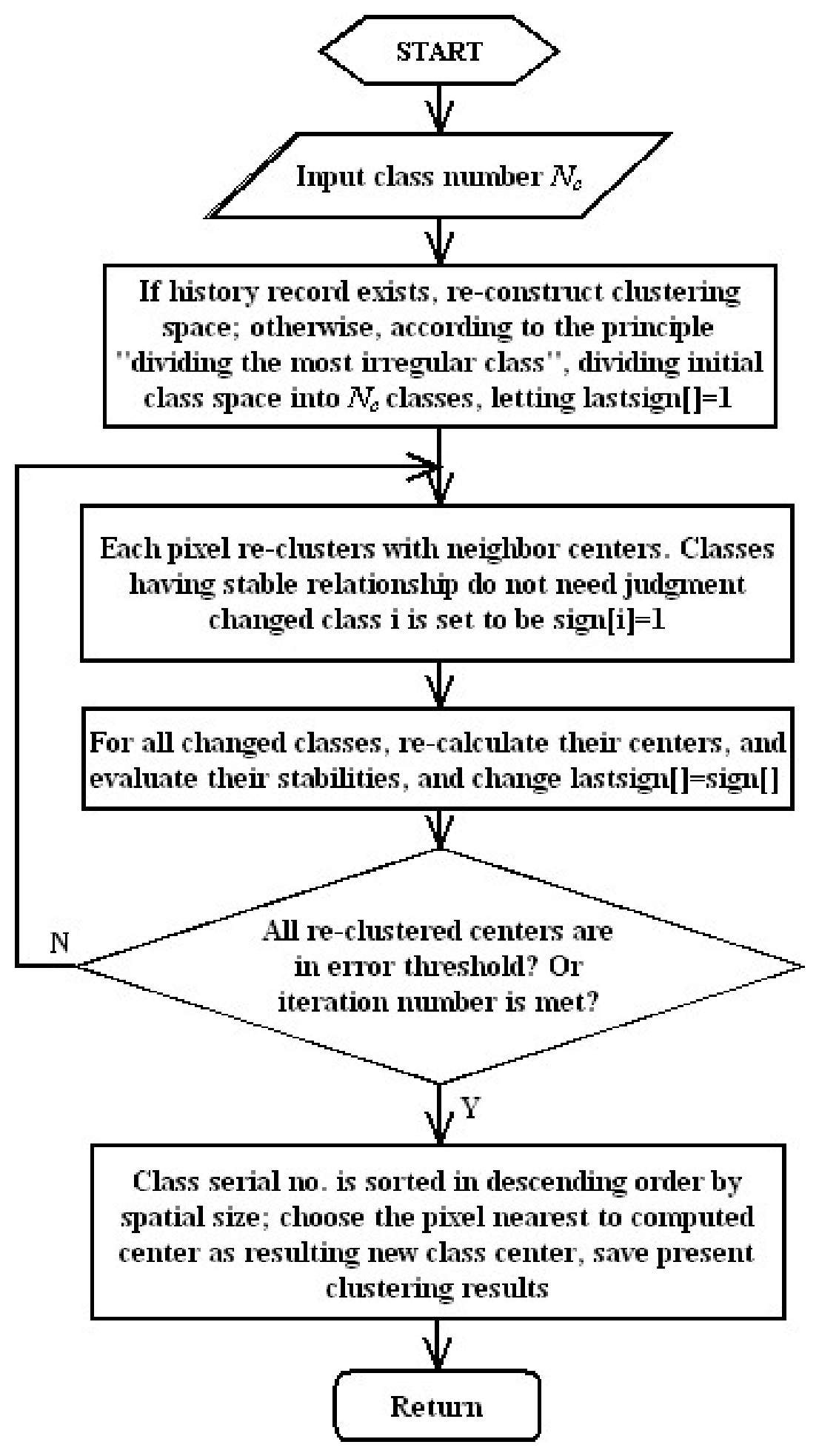
Figure 2.
Sketch map of class division and re-clustering for IKA. (a) The classCi is divided into two classes. (b) The pixel eij in class i is re-clustered by computing Euclidean distances with neighboring class centers (i and l).
Figure 2.
Sketch map of class division and re-clustering for IKA. (a) The classCi is divided into two classes. (b) The pixel eij in class i is re-clustered by computing Euclidean distances with neighboring class centers (i and l).
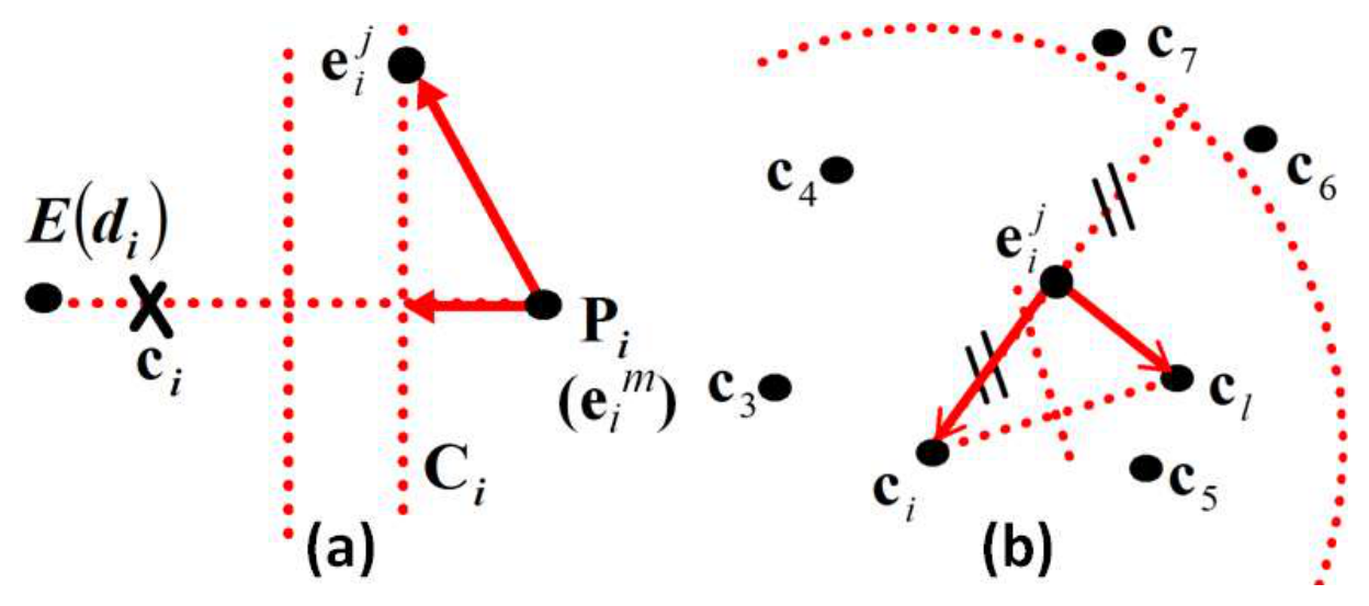
Figure 3.
(a) The sketch map of the intra-spectral residue data. (b) Space uniformity distribution of intra-class data under extreme division conditions.
Figure 3.
(a) The sketch map of the intra-spectral residue data. (b) Space uniformity distribution of intra-class data under extreme division conditions.
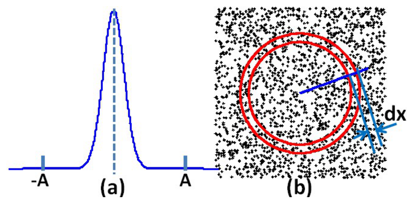
Figure 4.
Sook Lake AVIRIS hyperspectral images rebuilding results comparison: a. the 60th gray balanced band image, b. the 60th gray balanced band image rebuilt with 100 class centers created by the IKA clustering, where the intra-class pixels are present uniformly using their class center.
Figure 4.
Sook Lake AVIRIS hyperspectral images rebuilding results comparison: a. the 60th gray balanced band image, b. the 60th gray balanced band image rebuilt with 100 class centers created by the IKA clustering, where the intra-class pixels are present uniformly using their class center.
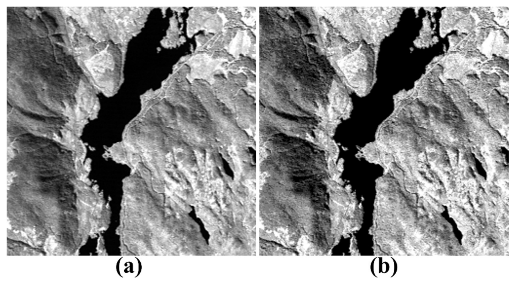
Figure 5.
Sook Lake AVIRIS images compression result: intra-class residue vs. class number (Nc). The size of intra-class residue B1 includes the sizes of the code and codebook, as determined by Huffman coding. The vertical axis represents the size of the intra-class residue, in Megabytes. The horizontal axis is the class number, ranging from 1 to 1780.
Figure 5.
Sook Lake AVIRIS images compression result: intra-class residue vs. class number (Nc). The size of intra-class residue B1 includes the sizes of the code and codebook, as determined by Huffman coding. The vertical axis represents the size of the intra-class residue, in Megabytes. The horizontal axis is the class number, ranging from 1 to 1780.
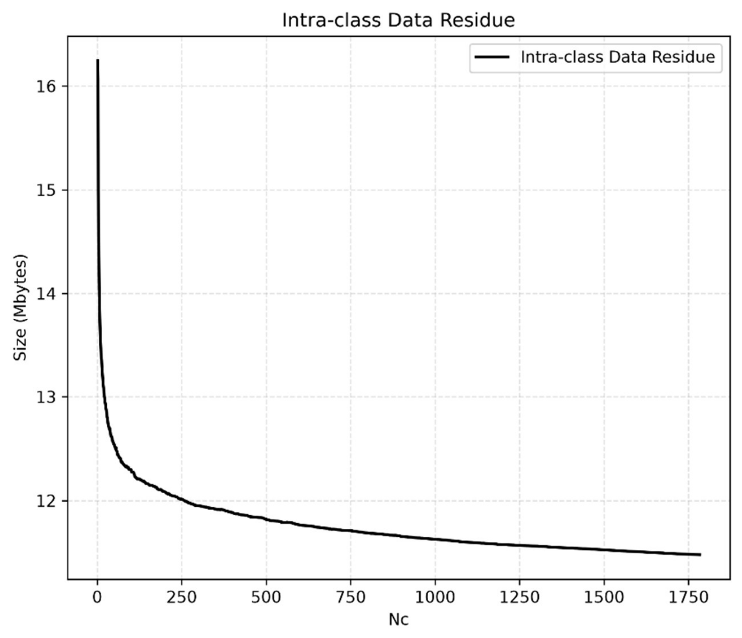
Figure 6.
Sook Lake AVIRIS images compression result: the residue of the class centers vs. class number (Nc). The size of the residue of the class centers, B2, includes the sizes of code and codebook using Huffman coding. The vertical axis is the size of the residue of the class centers, in Kilobytes. The horizontal axis is the class number, ranging from 1 to 1780.
Figure 6.
Sook Lake AVIRIS images compression result: the residue of the class centers vs. class number (Nc). The size of the residue of the class centers, B2, includes the sizes of code and codebook using Huffman coding. The vertical axis is the size of the residue of the class centers, in Kilobytes. The horizontal axis is the class number, ranging from 1 to 1780.
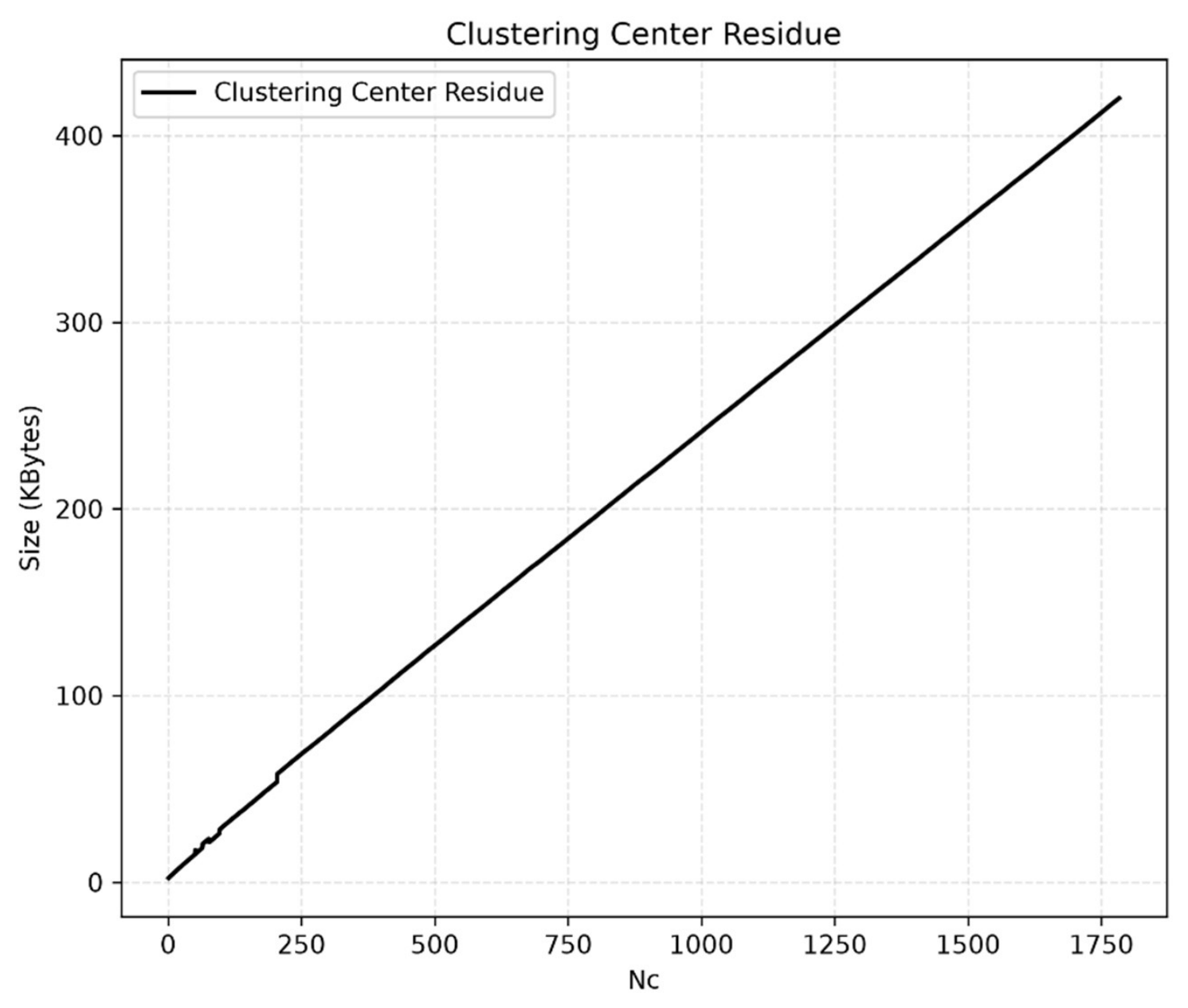
Figure 7.
Sook Lake AVIRIS images compression result: class map vs. class number (Nc). The size of class map B3 includes the sizes of code and codebook using Huffman coding. The vertical axis is the size of the class map, in Kilobytes. The horizontal axis is the class number, ranging from 1 to 1780.
Figure 7.
Sook Lake AVIRIS images compression result: class map vs. class number (Nc). The size of class map B3 includes the sizes of code and codebook using Huffman coding. The vertical axis is the size of the class map, in Kilobytes. The horizontal axis is the class number, ranging from 1 to 1780.
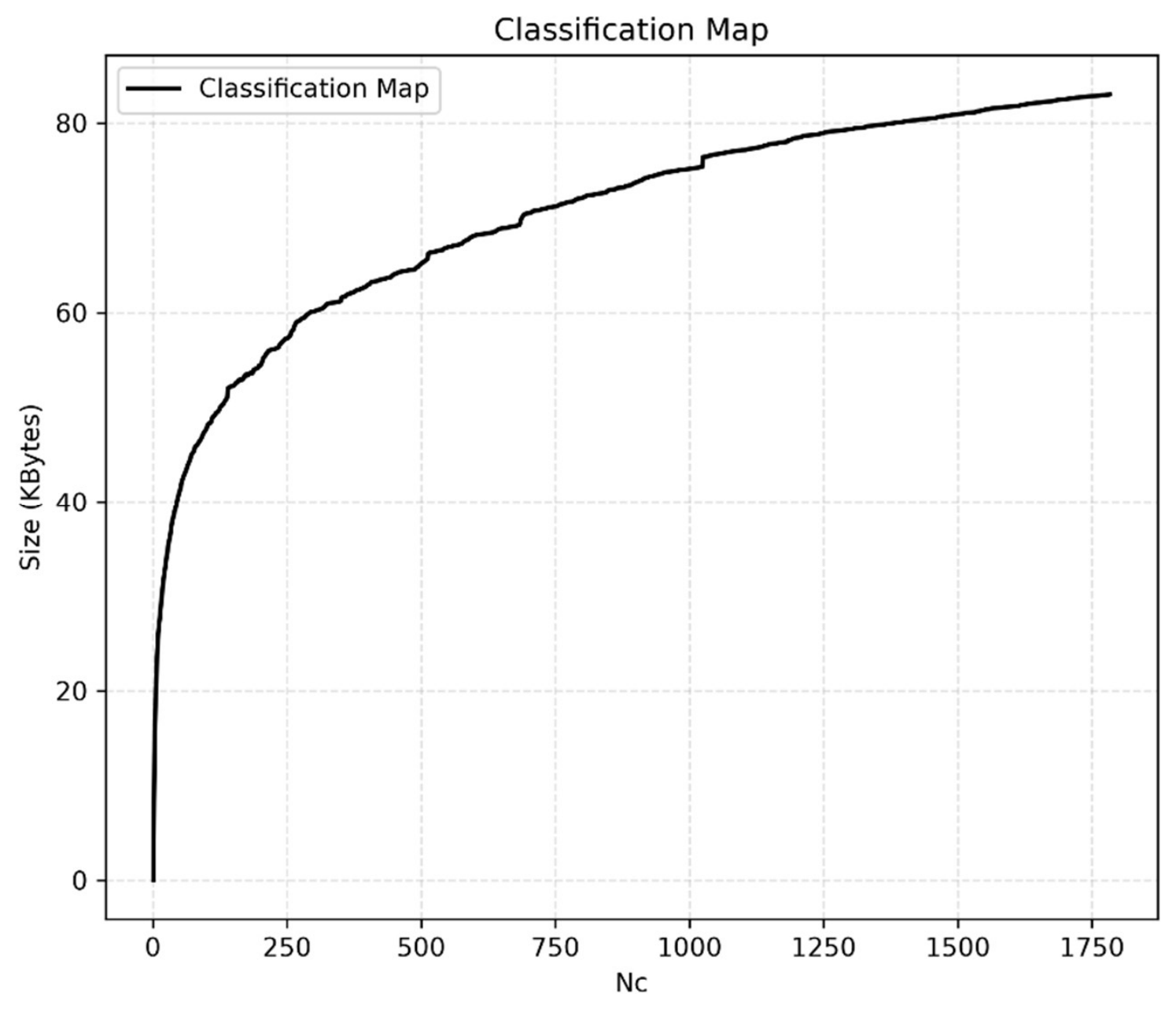
Figure 8.
Sook Lake AVIRIS images compression result: the total compressed data vs. class number (Nc). The total compressed data size includes the sizes of code and codebook for the class maps, clustering center residue, and intraclass residues, using Huffman coding. The vertical axis represents the size of the total compressed data, in Megabytes. The horizontal axis is the class number, ranging from 1 to 1780.
Figure 8.
Sook Lake AVIRIS images compression result: the total compressed data vs. class number (Nc). The total compressed data size includes the sizes of code and codebook for the class maps, clustering center residue, and intraclass residues, using Huffman coding. The vertical axis represents the size of the total compressed data, in Megabytes. The horizontal axis is the class number, ranging from 1 to 1780.
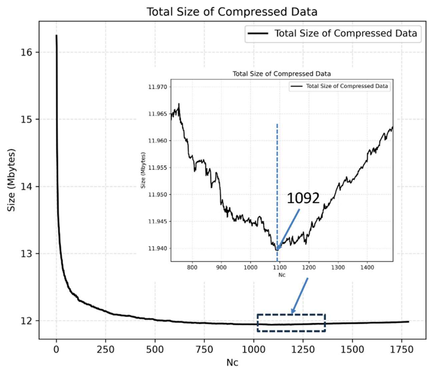
Figure 9.
Sook Lake AVIRIS images compression result: the LCR vs. class number (Nc). The vertical axis is the LCR without unit. The horizontal axis is the class number, ranging from 1 to 1780.
Figure 9.
Sook Lake AVIRIS images compression result: the LCR vs. class number (Nc). The vertical axis is the LCR without unit. The horizontal axis is the class number, ranging from 1 to 1780.
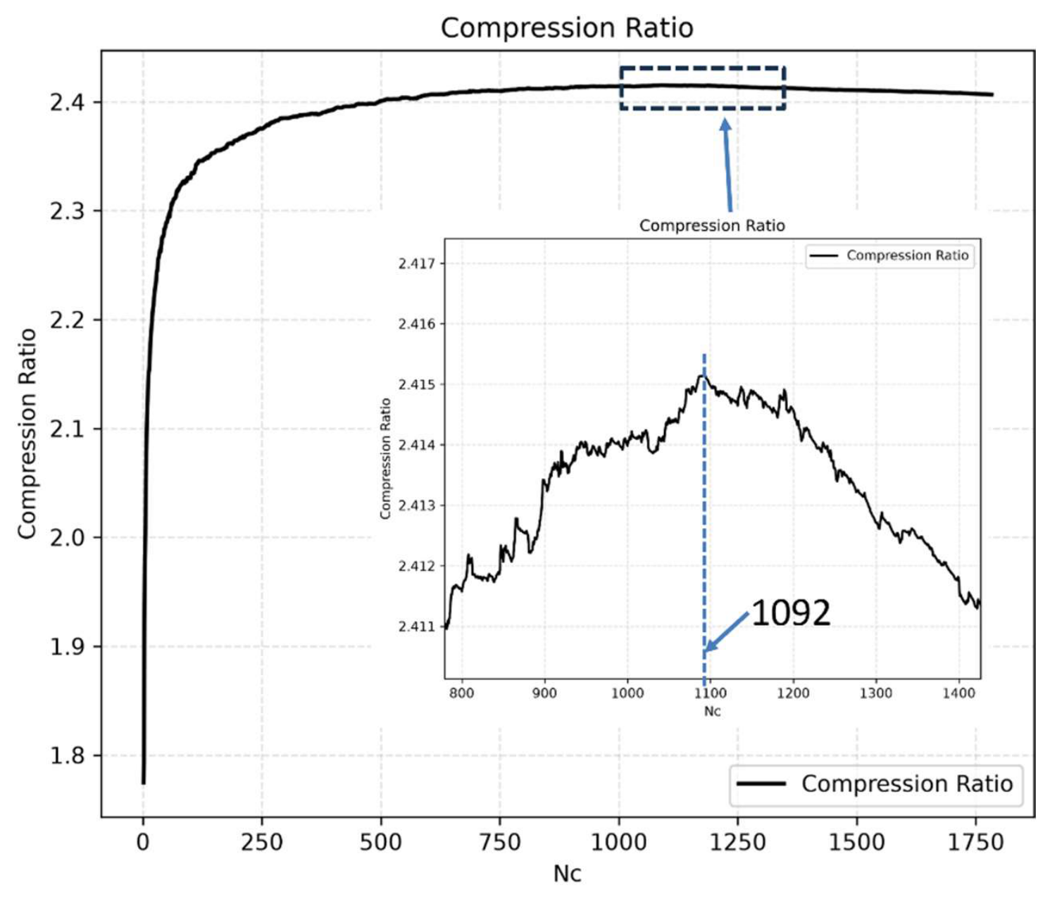

Table 1.
The execution process of LELCA, where the iteration number for clustering a class number has no limit, and the εc is set as 0.0001.
Table 1.
The execution process of LELCA, where the iteration number for clustering a class number has no limit, and the εc is set as 0.0001.
| Class no. Nc | Iteration number | Intra-class residue standard deviation σ1 | Spectral residue standard deviance σ2 | Lossless compression byte no. L | LCR | n1 | n2 | n3 | Ncbest | |
|---|---|---|---|---|---|---|---|---|---|---|
| 200 | 199 | 35.407818 | 230.068806 | 12214881 | 2.360714 | |||||
| 300 | 194 | 33.676117 | 231.546801 | 12121836 | 2.378834 | |||||
| 400 | 174 | 32.581664 | 232.651475 | 12075404 | 2.387981 | 200 | 300 | 400 | 1023 | |
| 1023 | 118 | 29.458689 | 232.382148 | 11959639 | 2.411096 | 300 | 400 | 1023 | 934 | |
| 934 | 98 | 29.763009 | 233.284102 | 11966192 | 2.409776 | 400 | 934 | 1023 | 1040 | |
| 1040 | 35 | 29.402593 | 232.143746 | 11958672 | 2.411291 | 934 | 1023 | 1040 | 1064 | |
| 1064 | 41 | 29.360868 | 231.907104 | 11962256 | 2.410569 | 934 | 1023 | 1040 | 1064 |
Table 2.
Compression results comparison.
| Algorithm | D2PCM | DPCM | CLCA/200 classes | LELCA/1040 classes |
|---|---|---|---|---|
| LCR | 1.9963 | 2.0525 | 2.3607 | 2.4113 |
Disclaimer/Publisher’s Note: The statements, opinions and data contained in all publications are solely those of the individual author(s) and contributor(s) and not of MDPI and/or the editor(s). MDPI and/or the editor(s) disclaim responsibility for any injury to people or property resulting from any ideas, methods, instructions or products referred to in the content. |
© 2026 by the authors. Licensee MDPI, Basel, Switzerland. This article is an open access article distributed under the terms and conditions of the Creative Commons Attribution (CC BY) license (http://creativecommons.org/licenses/by/4.0/).
Copyright: This open access article is published under a Creative Commons CC BY 4.0 license, which permit the free download, distribution, and reuse, provided that the author and preprint are cited in any reuse.


