

Submitted:
29 June 2026
Posted:
30 June 2026
You are already at the latest version
Abstract
Reduced air density at altitude challenges spark-ignition combustion in light-duty vehicles, particularly in Andean countries where fleets operate between sea level and over 4000~m~a.s.l. We quantified the effect of altitude on gasoline combustion efficiency and pollutant formation using 94,263 second-by-second records (2021–2025) from ten Euro~2–5 vehicles travelling Andean and coastal corridors in Ecuador (0--4000~m~a.s.l.). Emissions were measured with a Brain Bee AGS-688 analyser with pressure compensation; fuel consumption via OBD-II; operational demand via smoothed Vehicle Specific Power (\(\mathrm{PSV_{m10}}\)) in six K-Means clusters. We propose \(R_{\mathrm{CO}}=[\mathrm{CO}]/[\mathrm{CO_2}]\) and \(R_{\mathrm{HC}}=[\mathrm{HC}]/[\mathrm{CO_2}]\) as standardised, displacement-independent combustion quality indicators. \(R_{\mathrm{CO}}\) at 3500--4000~m exceeded the 500--1000~m value by 7.5\(\times\), and \(R_{\mathrm{HC}}\) by 18\(\times\). Nitric oxide showed a non-linear ``N''-pattern, peaking locally at 2000–2500~m (212~ppm) and absolutely at 3500–4000~m (613~ppm), linked to EGR suppression and rising chamber temperature. CO emission factors reached 6.42~g/km at 2000--2500~m versus 1.32~g/km at the coast (4.9\(\times\)). These results provide the first naturalistic evidence base for calibrating high-altitude emission inventories in Andean corridors.
Keywords:
altitude effect
; gasoline combustion
; real driving emissions
; CO/CO2 ratio
; Vehicle Specific Power
; Andean corridor
; Ecuador
1. Introduction
Road transport is one of the most relevant sources of urban air pollution worldwide, with light-duty gasoline vehicles being the primary emitters of carbon monoxide (CO), unburned hydrocarbons (HC) and nitrogen oxides (NOx) in most developing economies [1]. In Latin America, sustained fleet growth has intensified pressure on air quality in cities combining high vehicle density with severe topographic conditions [2]. In Ecuador, the light vehicle fleet exceeds three million units, of which over 60% are spark-ignition engines with fuel management calibrations lacking adaptive altitude compensation [3].
A first-order physical complication arises in countries with pronounced topographic relief: as altitude increases, atmospheric pressure decreases, reducing intake air density and the oxygen mass available for combustion per cycle [4,5]. In engines without adaptive altitude management—common in Euro 2 and Euro 3 calibrations—the shift of the air-fuel ratio towards richer mixtures produces incomplete oxidation of carbon and hydrogen, raising CO and HC in the exhaust [6,7,8]. This effect was documented in 1986 in Denver, Colorado (≈1600 m a.s.l.), where [9] showed that CO was the most altitude-sensitive pollutant fraction. [7] reported significant increases in CO and VOC between 0 and 3500 m in India; [10] measured, using PEMS, that CO and CO2 emission factors grow between 2270 and 4540 m on the Tibetan Plateau; and [11] quantified a CO increase of 2.56 times from 700 to 2400 m in China VI vehicles under RDE conditions.
The behaviour of nitric oxide (NO) with altitude is more complex. The reduction in peak cylinder temperature and the progressive suppression of exhaust gas recirculation (EGR) modify the Zeldovich thermal pathway [4]. [8] documented, using the MEDAS atmosphere simulator between 150 and 3000 m, that NOx grows up to 2000 m—where the EGR valve closes completely—and then stabilises or decreases. [11] report an “N”-shaped distribution with a peak at ≈1900 m, consistent with the present study’s findings. [12] found that road NOx can triple urban values in light-duty diesel vehicles at altitude.
Regarding fuel consumption, [13] systematically studied altitude–consumption interaction in a Euro 3 gasoline vehicle using an altimetric test bench, finding a non-monotonic effect: −3.5% in NEDC and +6.2% in Highway at 2200 m. [14] extended the analysis to 3030 m using a GT-Power model, showing that above 80 km/h and 2800 m engine performance deterioration outweighs aerodynamic resistance reduction. [15] confirm this behaviour via OBD-II data in naturalistic driving in the Ecuadorian Andean corridor.
The Real Driving Emissions (RDE) methodology, enabled by Portable Emission Measurement Systems (PEMS), has advanced the understanding of pollutant formation under real operating conditions [16,17,18]. However, most RDE studies have been conducted at altitudes below 1500 m [19,20], with only a small group on the Tibetan Plateau [10]. In Latin America, existing high-altitude studies are limited to diesel buses [18] or static measurements at a single altitude [3,21]. Studies covering 0–4000 in a single campaign with a naturalistic protocol, mixed Euro 2–5 fleet, and second-by-second recording are non-existent in the literature.
Vehicle Specific Power (VSP) has proven superior to approaches based solely on speed and acceleration for estimating real-world emission rates [17,22,23]. Its smoothed variant (10-s moving median) reduces sensitivity to GPS noise peaks [15,24]. Unlike the VSP bins of the MOVES model—whose inadequacy for mountainous terrain was demonstrated by [17]—K-Means clustering on yields empirically representative clusters of Andean conditions.
The ratios CO/ and HC/ have been proposed as robust combustion efficiency indicators normalised to fuel consumed [25], independent of engine displacement and dilution effects. [18] proposed fuel-based emission factors (, g/kg) with analogous logic for diesel buses, reducing inter-region variability by a factor of 3. The systematic extension to CO/ and HC/ stratified by altitudinal band has not been reported in the literature.
This study analyses 94263 second-by-second records (2021–2025) from ten light-duty Euro 2–5 vehicles in Ecuadorian Andean corridors between 0–4000 a.s.l. The specific objectives are:
- 1.
- To quantify the effect of altitude on CO, , HC and NO along a continuous 4000 m gradient under real driving conditions.
- 2.
- To characterise how operational demand (, 6 K-Means clusters) modulates the altitude–emission relationship.
- 3.
- To evaluate fuel consumption as a function of altitude and operational demand using OBD-II data.
- 4.
- To propose and validate and as standardised combustion quality indicators by altitudinal band for mixed Euro-standard fleets.
2. Materials and Methods
2.1. Study Area and Road Corridors
Data were collected along three interconnected road corridors in Ecuador spanning from sea level to ≈4000 m a.s.l. (Figure 1). The corridors cross the Pacific coastal plain, the inter-Andean valley and the high-altitude paramo, including urban, peri-urban and rural segments. Within less than 200 km, atmospheric pressure drops from 101.3 to 61.6 kPa [5], a gradient comparable to the Tibetan Plateau [10] but additionally covering low altitudes (0–800 m) absent in all previous Latin American Andean studies. Instrumented routes included: Riobamba–Guano, Riobamba–Chimborazo, Riobamba–Santo Domingo, Riobamba–Guayaquil and Santo Domingo–El Carmen.
2.2. Test Vehicle Fleet
Ten light-duty gasoline vehicles were instrumented according to the criteria: (i) displacement 1000–2500; (ii) Euro 2–5 emission standard; (iii) OBD-II compliance; (iv) regular operational use on the study corridors during 2021–2025. The deliberate inclusion of Euro 2–5 vehicles—unlike studies with homogeneous fleets [11,17]—allows evaluation of the moderating effect of emission control technology on the altitudinal response (Table 1).
2.3. Measurement Equipment and Data Acquisition
2.3.1. Exhaust Gas Analyser
Exhaust gas concentrations were measured with a Brain Bee AGS-688 analyser (Brain Bee S.p.A., Parma, Italy) operating via NDIR for CO, and HC (n-hexane equivalent), and electrochemical sensor for NO. The instrument complies with ISO 3930/OIML Class 0 and Directive 2004/22/EC. It incorporates automatic ambient pressure compensation between 85.0 and 106.0 kPa, covering the entire altitudinal gradient of the study—unlike conventional PEMS used in similar studies [17,18] that require external barometric corrections. Data were recorded at 1 Hz via RS-232 (Table 2).
2.3.2. OBD-II Fuel Consumption and Vehicle Kinematics
Instantaneous fuel consumption was acquired via OBD-II PID 0x5E (Engine Fuel Rate, L/h). This methodology showed R2 correlation with gravimetric measurements in high-altitude buses [18]. The signal was synchronised with the gas analyser to ±0.5 s. Vehicle speed was obtained from OBD-II (PID 0x0D) and GPS; instantaneous acceleration was calculated as a first-order finite difference filtered with a 3-s moving average [17].
2.4. Data Collection Protocol
2.5. Data Quality Control
A total of 94263 valid records in the 0–4000 range were obtained after the following filters:
- (1)
- Exclusion of cold-start (coolant <80 °C).
- (2)
- Removal of saturations: CO >9.5 % vol or HC >9500 ppmvol.
- (3)
- Exclusion of GPS altitude outside 0–4100 m a.s.l.
- (4)
- Removal of duplicate timestamps and implausible acceleration ( m ).
- (5)
- Discard of records with <2 % vol.
2.6. Vehicle Specific Power and Operational Clustering
2.6.1. Definition of
VSP is defined as [22]:
where v (m/s) is speed, a (m/s2) acceleration, , m/s2, (rad) road grade, , air density, aerodynamic coefficient, (m2) frontal area and m (kg) kerb mass. The 10-s moving median:
confers robustness against GPS noise peaks [24]. Air density was estimated second-by-second using the ISA model [5]:
with kg/m3, K, K/m.
2.6.2. K-Means Clustering
The dataset was segmented into six clusters using K-Means on and instantaneous acceleration, both standardised. The optimal was determined with the elbow criterion and silhouette coefficient. Clusters were labelled: Idle/stopped, Deceleration, Light cruise, Positive acceleration, High demand and Maximum demand, following the taxonomy of [23].
2.7. Combustion Quality Indicators
2.8. Altitudinal Band Stratification and Statistical Analysis
The altitudinal range was divided into eight 500-m bands (Table 3). Differences between bands and clusters were assessed with Kruskal–Wallis followed by Dunn pairwise comparison with Bonferroni correction [17]. Effect sizes were quantified with Cliff’s ; altitude–emission correlations with Spearman’s . Analysis in Python 3.11. Significance level: .
3. Results
3.1. Dataset Description
The final dataset comprised 94263 second-by-second records distributed across eight altitudinal bands (Table 4). The 2500–3000 m band concentrated the most records (22834; 24.2%), followed by the 0–500 m band (21882; 23.2%). Light cruise was the predominant operational mode (27966 records; 29.7%).
3.2. Combustion Quality Indicators: and
Both ratios showed statistically significant differences across bands (Kruskal–Wallis: , for ; , for ). Table 5 presents medians and IQR by band; Figure 2 shows the full distributions.
reached its highest value in the 3500–4000 m band (median ), 7.5 times the value of the 500–1000 m band (), with medium effect size ( between 0–500 m and 500–1000 m). in the 2000–2500 m band (0.0018) exceeded the 500–1000 m value (0.0001) by 18 times. Both indicators showed a non-monotonic pattern with relative minima in the 500–1000 m and 2500–3000 m bands.
3.3. Relationship Between Lambda and Altitude
The air-fuel ratio () showed significant differences across bands (, ), with small effect sizes (). Spearman correlation between altitude and was negative and significant in high-demand clusters: High demand (, ) and Maximum demand (, ), indicating mixture enrichment under high load at altitude. The correlation was virtually null in Positive acceleration (, ). Figure 3 shows the heatmap by band and cluster.
3.4. Volumetric Exhaust Gas Concentrations
Table 6 summarises median volumetric concentrations by band. Figure 4 illustrates altitudinal trends.
Carbon monoxide (CO). Median CO increased from the absolute minimum of 0.08 %vol in the 500–1000 m band to 0.77 %vol in the 3500–4000 m band (9.6×).
Unburned hydrocarbons (HC). The 2000–2500 m band recorded the highest median HC (188 ppm), 12.5 times the minimum of the 500–1000 m band (15 ppm).
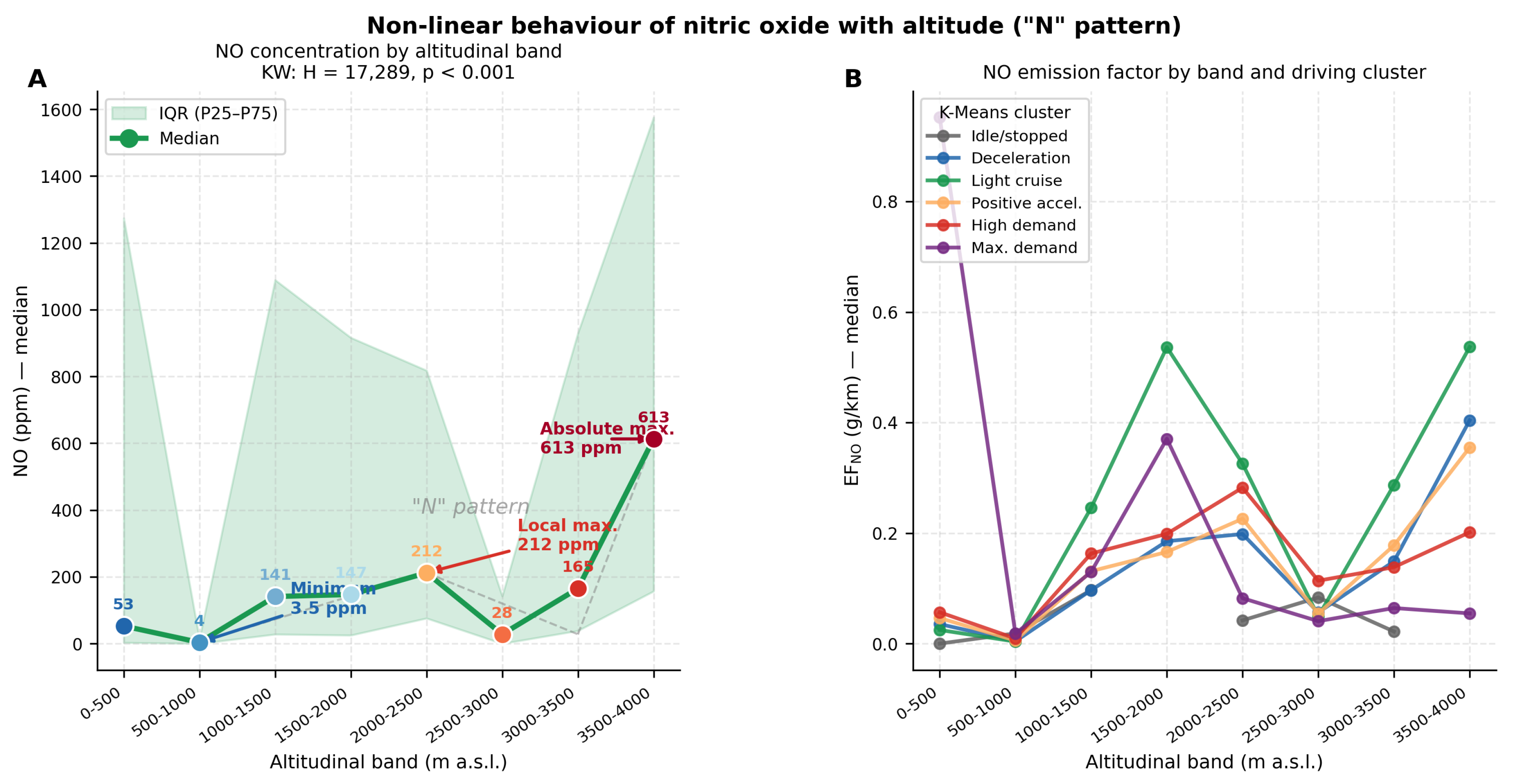
Nitric oxide (NO). NO exhibited the most pronounced non-linear behaviour (, ). From a minimum of 3.5 ppm in 500–1000 m, concentrations rose to 212 ppm in 2000–2500 m, then fell to 28 ppm in 2500–3000 m and rose again to the absolute maximum of 613 ppm in 3500–4000 m. This “N”-pattern is discussed in Section 4.
Figure 5.
Non-linear behaviour of nitric oxide with altitude. Panel A: median NO concentration with shaded IQR; arrows mark the minimum (3.5 ppm at 500–1000 m), local maximum (212 ppm at 2000–2500 m) and absolute maximum (613 ppm at 3500–4000 m). Panel B: NO emission factor (g/km) by altitudinal band and K-Means driving cluster.
Figure 5.
Non-linear behaviour of nitric oxide with altitude. Panel A: median NO concentration with shaded IQR; arrows mark the minimum (3.5 ppm at 500–1000 m), local maximum (212 ppm at 2000–2500 m) and absolute maximum (613 ppm at 3500–4000 m). Panel B: NO emission factor (g/km) by altitudinal band and K-Means driving cluster.
Carbon dioxide (CO2). CO2 concentrations remained relatively stable (range: 11.10–12.10 %vol; 9% relative variation), confirming that the ECU maintains overall stoichiometric control.
3.5. Emission Factors by Altitudinal Band
Emission factors (EF, g/km) showed significant differences across bands for all gases (CO: ; CO2: ; HC: ; NO: ; all ). Table 7 consolidates EF medians and fuel consumption. Figure 6 disaggregates EF by K-Means cluster.
EFCO peaked in the 2000–2500 m band (6.42 g/km), 4.9 times the minimum of the 500–1000 m band (1.32 g/km). EFNO showed the most pronounced behaviour: from 0.01 g/km in 500–1000 m to 0.36 g/km in 3500–4000 m (36 times). EFCO2 showed a decreasing trend with altitude, from 227.9 g/km (500–1000 m) to 112.7 g/km (3500–4000 m), consistent with reduced aerodynamic resistance at lower air density.
3.6. Fuel Consumption by Altitudinal Band
Fuel consumption showed significant differences (, ), with small consecutive-band effect sizes (). Median ranged from 7.97 L/100 km (1000–1500 m) to 11.56 L/100 km (1500–2000 m). Spearman correlations revealed mode-dependent effects: High demand showed positive correlation (, ), while Light cruise () and Positive acceleration () showed negative correlations (both ).
4. Discussion
4.1. Combustion Quality Along the Altitudinal Gradient
The and ratios proved to be sensitive and standardised indicators of combustion quality deterioration with altitude. The 7.5-fold increase in between the 500–1000 m and 3500–4000 m bands exceeds the 2.56-fold factor reported by [11] for absolute CO in the 700–2400 m range in China VI vehicles, and the 2–3-fold increase reported by [7] between 0 and 3500 m in India. The superiority of as an indicator lies in that, by normalising to CO2, it eliminates confounding from displacement, exhaust mass flow and barometric dilution effects at high altitude [25]. This approach is analogously superior to the factors proposed by [18] for diesel buses, extending it now to gasoline vehicles and continuous altitudinal gradients.
The non-monotonic pattern—with relative minima in the 500–1000 m and 2500–3000 m bands—reflects the interaction between route driving profiles and the altitude response of fuel management. The 500–1000 m band corresponds mainly to the coastal Riobamba–Guayaquil route, where the predominance of Light cruise mode at moderate speeds favours complete combustion regardless of altitude. This phenomenon is consistent with observations by [18] in diesel buses on Mexican mountain highways, where CO emission factors were significantly lower on the highway corridor than in urban areas despite higher altitude, due to a more efficient driving profile.
4.2. Non-Linear Behaviour of Nitric Oxide
The “N”-pattern of NO—minimum at 500–1000 m (3.5 ppm), local maximum at 2000–2500 m (212 ppm), descent to 28 ppm at 2500–3000 m, and absolute maximum at 3500–4000 m (613 ppm)—constitutes the most original finding of this study for three reasons. First, its magnitude: the absolute maximum of 613 ppm exceeds the minimum by 175 times and is 2.9 times the sea-level value (52.7 ppm at 0–500 m). Second, its altitudinal range: previous studies in gasoline reported the NOx peak up to ≈1900 m in China VI vehicles [11] or up to 2000 m in diesel engines with the MEDAS simulator [8]; this study documents for the first time a second absolute maximum above 3500 m. Third, the nature of the gradient: while previous studies used static conditions or regulated cycles, the data presented here correspond to naturalistic driving, eliminating cycle bias.
The underlying mechanism can be explained by the superposition of two opposing effects. On one hand, the reduction of partial oxygen pressure decreases peak flame temperature and thereby the Zeldovich thermal NO formation rate [4]. On the other hand, progressive EGR suppression—documented by [8] from 2000 m in Euro 4 engines—increases chamber temperature by eliminating inert gas mass from the cycle, favouring NO formation. At extreme altitudes (>3000 m), the second effect outweighs the first, especially in Euro 2–3 fleet vehicles without adaptive compensation, explaining the second maximum at 3500–4000 m.
4.3. Fuel Consumption and Operational Demand
Fuel consumption did not follow a monotonic trend with altitude, in line with observations of [13] for a Euro 3 vehicle on an altimetric test bench and [14] using GT-Power up to 3030 m. The consumption minimum at 1000–1500 m (7.97 L/100 km) and maximum at 1500–2000 m (11.56 L/100 km) reflect the interaction among: aerodynamic resistance reduction with lower air density [13], progressive mixture enrichment increasing fuel flow rate, and additional mechanical demand on steep Andean gradients.
Cluster analysis revealed a key dependency: the altitude–consumption correlation changes sign between clusters. In High demand the correlation is positive (), while in Light cruise it is negative (), consistent with aerodynamic resistance reduction proportional to [14]. This result demonstrates that studies not controlling the operational mode produce consumption estimates that mix opposing effects and are inconsistent across corridors with different mode compositions.
4.4. Implications for High-Altitude Emission Inventories
Results have direct implications for Andean emission inventory construction. Standard EF values used in tools such as MOVES or COPERT—derived from regulated low-altitude cycles—significantly underestimate CO and HC emissions in the 1500–4000 m range. The maximum EFCO (6.42 g/km at 2000–2500 m) is 4.9 times the coastal minimum (1.32 g/km at 500–1000 m), and [18] found similarly that CO emission factors for diesel buses in Mexico (>2000 m) were 3 times IPCC reference values. Using and stratified by altitudinal band and operational cluster provides a normalised, easily replicable alternative to update these inventories without exhaust mass flow measurement.
4.5. Study Limitations
Main limitations include: (i) the ten-vehicle fleet, while deliberately representing the Euro 2–5 spectrum of the Ecuadorian fleet, does not allow statistically robust stratification by Euro standard independently; (ii) the Brain Bee AGS-688 operates as an exhaust pipe probe rather than a dilution PEMS, excluding absolute mass emission calculations with the precision of equipment such as the Semtech ECOSTAR [18]; (iii) driving routes are limited to three Ecuadorian corridors; and (iv) ambient temperature effects—which co-vary with altitude in Andean corridors—were not explicitly decoupled in the statistical analysis.
5. Implications for Carbon and Pollutant Reduction in Combustion Applications
The findings of this study carry direct implications for ongoing efforts to reduce carbon, NOx and SOx-related emissions from existing and emerging combustion applications, particularly in regions where engines and combustion systems operate under variable air density.
5.1. Altitude as an Overlooked Variable in Carbon Reduction Strategies
Most decarbonisation roadmaps for the light-duty fleet—fuel reformulation, hybridisation, or fleet renewal schedules—are calibrated using emission factors derived from sea-level or near-sea-level test cycles. Our results show that EFCO2 is not the limiting concern at altitude; rather, it decreases moderately with elevation due to reduced aerodynamic load (Table 7). The critical risk lies instead in the substantial underestimation of CO and HC emission factors above ≈2000 m a.s.l., where EFCO reaches 6.42 g/km—4.9 times the coastal reference value. Carbon-reduction policies that rely on low-altitude EF values to project co-benefits in criteria pollutant reduction will therefore systematically underestimate the air-quality burden of the existing gasoline fleet in Andean and other high-altitude regions, weakening the evidence base for prioritising fleet renewal or retrofit programmes in these areas.
5.2. A Critical Altitude Threshold for Combustion Control Intervention
The pronounced increase in and beyond 2000 m, and the divergence of the NO “N”-pattern above 3000 m, identify ≈2000 m a.s.l. (≈79 kPa) as the altitude at which conventional spark-ignition combustion control— particularly in Euro 2–3 vehicles without adaptive fuelling or EGR modulation—loses effectiveness in maintaining low-emission combustion. This threshold provides a quantitative target for prioritising interventions such as: (i) adaptive air-fuel ratio control recalibrated for barometric pressure rather than fixed look-up tables; (ii) EGR systems designed to remain partially active at high altitude rather than fully closing near 2000 m, to limit the NO rebound documented at 3500–4000 m; and (iii) accelerated electrification or hybridisation incentives specifically targeted at fleets operating above this threshold, where the combustion-based emission penalty is largest and the relative benefit of electrified powertrains is correspondingly highest.
5.3. Transferability to Broader Combustion Systems
While this study focuses on light-duty gasoline engines, the underlying physical driver—reduced oxidant availability and altered thermal conditions at lower ambient pressure—is not unique to road vehicles. The / framework, normalised to CO2 and therefore independent of fuel flow or dilution, is in principle transferable to any combustion system operating under variable air density or oxidant supply, including stationary generators at high elevation, dual-fuel and marine engines subject to variable intake conditions, and combustion-based heating systems in high-altitude communities. In all these applications, the same diagnostic logic applies: monitoring CO/CO2 and HC/CO2 ratios offers a low-cost, mass-flow-independent indicator of combustion quality degradation that can flag when a system is operating outside its designed efficiency envelope—supporting earlier and more targeted interventions to reduce carbon and criteria pollutant emissions across the broader landscape of combustion applications addressed by this Special Issue.
6. Conclusions
This study presents the first naturalistic evidence at the Andean corridor scale of the effect of altitude on combustion efficiency and emissions of light-duty gasoline vehicles in the 0–4000 a.s.l. range, based on 94263 second-by-second records from a mixed Euro 2–5 fleet in Ecuador. The main conclusions are:
- 1.
- The ratios and are effective standardised indicators of combustion quality at altitude. increased 7.5 times between the coastal 500–1000 m band and the 3500–4000 m band, and by 18 times. Their implementation does not require exhaust mass flow measurement, making them accessible for fleet monitoring in middle-income countries.
- 2.
- Nitric oxide exhibits a non-linear “N”-pattern with an absolute maximum at 3500–4000 m. Median NO concentration reached 613 ppm—175 times the minimum of 3.5 ppm at 500–1000 m— as a result of the interplay between EGR suppression and reduction of partial oxygen pressure. This pattern, documented here for the first time in gasoline over a continuous 4000 m gradient, implies that low-altitude NOx limits are insufficient to characterise real impact in high mountain areas.
- 3.
- The operational mode regulates the intensity of the altitudinal effect on consumption and emissions. The altitude–consumption correlation changed sign between High demand () and Light cruise (), and the altitude– correlation was virtually null in Positive acceleration (, ) but significant in High demand (, ). This demonstrates that studies not controlling operational demand produce ambiguous estimates of the altitudinal effect.
- 4.
- CO emission factors in the 2000–2500 m band are 4.9 times the coastal values. EFCO reached 6.42 g/km at 2000–2500 m versus 1.32 g/km at 500–1000 m. This threshold of ≈2000 m a.s.l., where pressure drops to ≈79 kPa, represents the critical point from which Euro 2–3 engines without adaptive compensation lose stoichiometric control, and should be considered as an operational limit in national regulations of Andean countries.
- 5.
- Fuel consumption does not follow a monotonic trend with altitude. Variation between 7.97 L/100 km (1000–1500 m) and 11.56 L/100 km (1500–2000 m) reflects competition between aerodynamic resistance reduction at lower air density and increased fuel expenditure to compensate engine performance loss, confirming the findings of [13] and [14] in bench and model conditions and extending them to the Andean naturalistic context.
These results provide the first naturalistic evidence base for the calibration of emission inventory models in Andean corridors and for informing vehicle fleet renewal policies in countries with high altitudinal exposure. Future work should address explicit decoupling of temperature and altitude effects, Euro-standard stratification with larger samples, and extension of the / methodology to diesel, hybrid and natural gas vehicles.
Author Contributions
Conceptualisation, P.A.M.-P.; methodology, P.A.M.-P. and E.A.-P.; software, P.A.M.-P. and J.C.; validation, J.C. and A.V.R.-C.; formal analysis, P.A.M.-P.; investigation, P.A.M.-P., E.A.-P. and V.D.B.-M.; data curation, J.C. and V.D.B.-M.; writing—original draft, P.A.M.-P.; writing—review and editing, all authors; visualisation, P.A.M.-P. and A.V.R.-C.; supervision, P.A.M.-P. All authors have read and agreed to the published version of the manuscript.
Funding
This research received no external funding.
Data Availability Statement
The dataset supporting the conclusions of this article is available from the corresponding author upon reasonable request.
Conflicts of Interest
The authors declare no conflicts of interest.
References
- World Health Organization. Ambient Air Quality Database 2022; Technical report; WHO, 2022. [Google Scholar]
- UNEP. Used Vehicles and the Environment; Technical report; United Nations Environment Programme, 2021. [Google Scholar]
- Sánchez-Mendoza, A.; Vinueza-Morales, M.; Alcázar-Espinoza, J.; Pineda-Silva, G.; Aucay-García, I. Gasoline Vehicle Emissions at High Altitude: An Exploratory STATIS Study in Guaranda, Ecuador. Atmosphere 2025, 16, 281. [Google Scholar] [CrossRef]
- Heywood, J.B. Internal Combustion Engine Fundamentals; McGraw-Hill, 1988. [Google Scholar]
- ISO 2533:1975; Standard Atmosphere. Technical report; International Organization for Standardization, 1975.
- Zhao, L.; Wang, X.; Ge, Y. Effect of high altitude on exhaust emissions of gasoline vehicles during real driving. Sci. Total Environ. 2020, 723, 138008. [Google Scholar] [CrossRef] [PubMed]
- Nagpure, A.S.; Gurjar, B.R.; Kumar, P. Impact of altitude on emission rates of ozone precursors from gasoline-driven light-duty commercial vehicles. Atmos. Environ. 2011, 45, 1413–1417. [Google Scholar] [CrossRef]
- Bermúdez, V.; Serrano, J.R.; Piqueras, P.; Gómez, J.; Bender, S. Analysis of the role of altitude on diesel engine performance and emissions using an atmosphere simulator. Int. J. Engine Res. 2017, 18, 105–117. [Google Scholar] [CrossRef]
- Miron, W.L.; Ragazzi, R.A.; Hollman, T.W.; Gallagher, G.L. Ethanol-Blended Fuel as a CO Reduction Strategy at High Altitude; Technical Report 860530; SAE International, 1986. [Google Scholar] [CrossRef]
- Qi, Z.; Gu, M.; Cao, J.; Zhang, Z.; You, C.; Zhan, Y.; Ma, Z.; Huang, W. The Effects of Varying Altitudes on the Rates of Emissions from Diesel and Gasoline Vehicles Using a PEMS. Atmosphere 2023, 14, 1739. [Google Scholar] [CrossRef]
- Wang, J.; Wang, L.; Li, J.; Li, J.; Xu, F.; Han, F.; He, J.; Chen, Q.; Chen, X. RDE and dynamometer analysis of light-duty vehicle emissions across altitudes, temperatures, and driving styles. PLoS ONE 2025, 20, e0318298. [Google Scholar] [CrossRef] [PubMed]
- Ramos, Á.; García-Contreras, R.; Armas, O. Performance, combustion timing and emissions from a light duty vehicle at different altitudes fueled with animal fat biodiesel, GTL and diesel fuels. Appl. Energy 2016, 182, 507–517. [Google Scholar] [CrossRef]
- Zervas, E. Impact of altitude on fuel consumption of a gasoline passenger car. Fuel 2011, 90, 2340–2342. [Google Scholar] [CrossRef]
- Hao, L.; Wang, C.; Yin, H.; Hao, C.; Wang, H.; Tan, J.; Wang, X.; Ge, Y. Model-based estimation of light-duty vehicle fuel economy at high altitude. Adv. Mech. Eng. 2019, 11, 1–10. [Google Scholar] [CrossRef]
- Montúfar-Paz, P.A.; Cuisano, J.C. Development and Validation of a Methodology for Predicting Fuel Consumption and Emissions in Light Vehicles Based on Clustering of Instantaneous and Cumulative Vehicle Power. Vehicles 2025, 7, 16. [Google Scholar] [CrossRef]
- Andreae, M.M.; et al. Real-world driving emission measurement methodologies: A critical review of PEMS-based studies. Transp. Res. Part D. 2022, 108, 103333. [Google Scholar] [CrossRef]
- Zhang, L.; Hu, X.; Qiu, R.; Lin, J. Comparison of real-world emissions of LDGVs of different vehicle emission standards on both mountainous and level roads in China. Transp. Res. Part D. 2019, 69, 24–39. [Google Scholar] [CrossRef]
- Giraldo, M.; Huertas, J.I. Real emissions, driving patterns and fuel consumption of in-use diesel buses operating at high altitude. Transp. Res. Part D. 2019, 77, 21–36. [Google Scholar] [CrossRef]
- Wang, J.; Wang, L.; Li, J.; et al. Comparison of vehicular emissions at different altitudes: Characteristics and policy implications. Environ. Pollut. 2025, 366, 125000. [Google Scholar] [CrossRef]
- Jiang, Z.; Wu, L.; Niu, H.; et al. Investigating the impact of high-altitude on vehicle carbon emissions: A comprehensive on-road driving study. Sci. Total Environ. 2024, 921, 170671. [Google Scholar] [CrossRef] [PubMed]
- Garcia Tobar, M.; Cabrera Ojeda, O.; et al. Impact of Oil Viscosity on Emissions and Fuel Efficiency at High Altitudes. Lubricants 2024, 12, 277. [Google Scholar] [CrossRef]
- Jiménez-Palacios, J.L. Understanding and Quantifying Motor Vehicle Emissions with Vehicle Specific Power and TILDAS Remote Sensing. PhD Thesis, Massachusetts Institute of Technology, 1999. [Google Scholar]
- Bhoopalam, A.K.; et al. Influence of driving patterns on vehicle emissions: A case study for Latin American cities. Transp. Res. Part D. 2016, 43, 29–40. [Google Scholar] [CrossRef] [PubMed]
- Rosero, F.; Rosero, C.X.; Segovia, C. Towards Simpler Approaches for Assessing Fuel Efficiency and CO2 Emissions Using On-Board Diagnostic Data. Energies 2024, 17, 4814. [Google Scholar] [CrossRef]
- Jiang, W.; et al. Distribution characteristics of CO and NOx in RDE tests using CO/CO2 and NOx/CO2 as combustion quality indicators. Transp. Res. Part D. 2024, 130, 104200. [Google Scholar] [CrossRef]
Figure 1.
Altitudinal profiles of instrumented road corridors in Ecuador (2021–2025). The upper panel shows all corridors superimposed; individual panels show each corridor coloured by altitudinal band. Dashed horizontal lines mark critical pressure thresholds at 2000 m (≈79 kPa) and 3000 m (≈70 kPa).
Figure 1.
Altitudinal profiles of instrumented road corridors in Ecuador (2021–2025). The upper panel shows all corridors superimposed; individual panels show each corridor coloured by altitudinal band. Dashed horizontal lines mark critical pressure thresholds at 2000 m (≈79 kPa) and 3000 m (≈70 kPa).
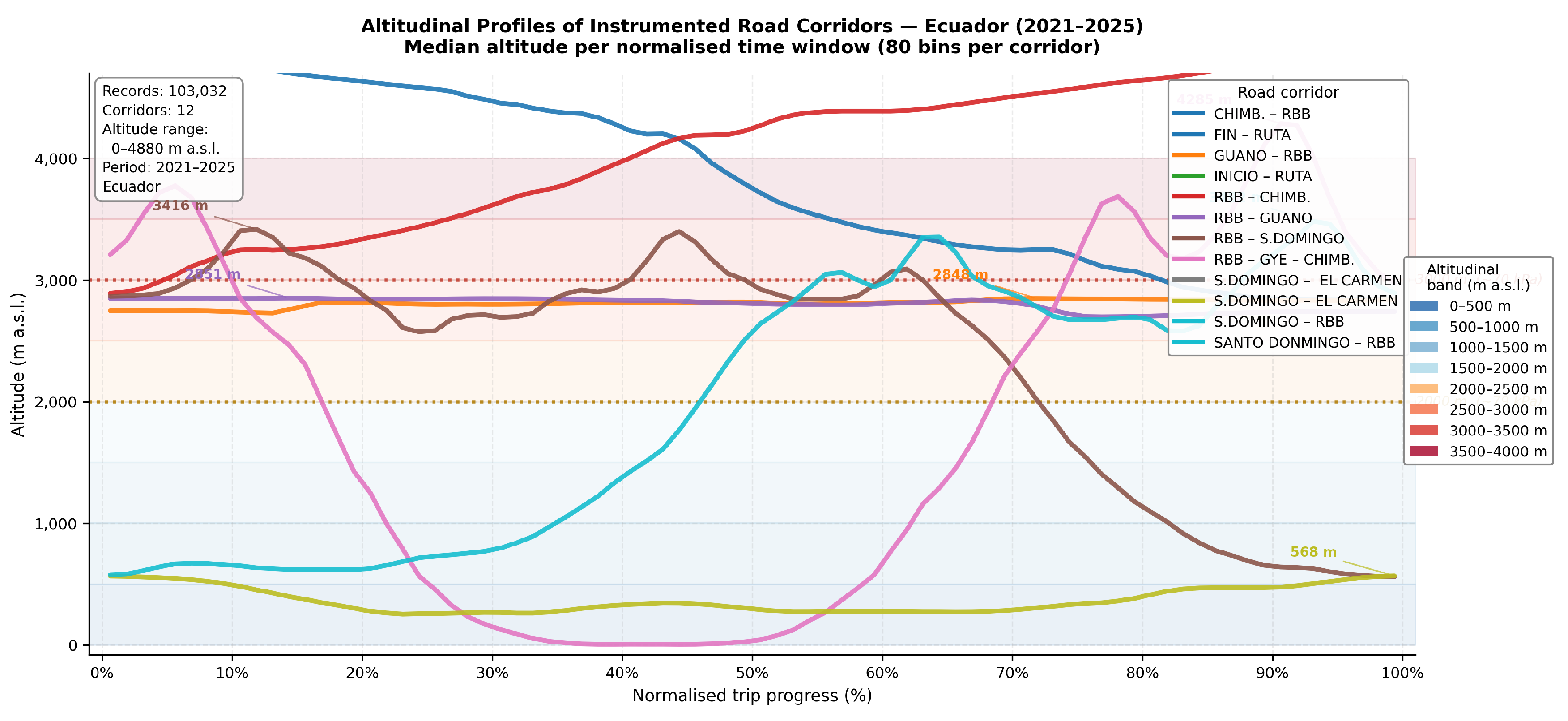
Figure 2.
Distribution of combustion quality ratios (panel A) and (panel B) by altitudinal band. Boxes represent IQR; central line is median; whiskers extend to 1.5×IQR. Bold values indicate medians. Colours follow the altitudinal gradient from blue (low altitude) to red (high altitude). records.
Figure 2.
Distribution of combustion quality ratios (panel A) and (panel B) by altitudinal band. Boxes represent IQR; central line is median; whiskers extend to 1.5×IQR. Bold values indicate medians. Colours follow the altitudinal gradient from blue (low altitude) to red (high altitude). records.
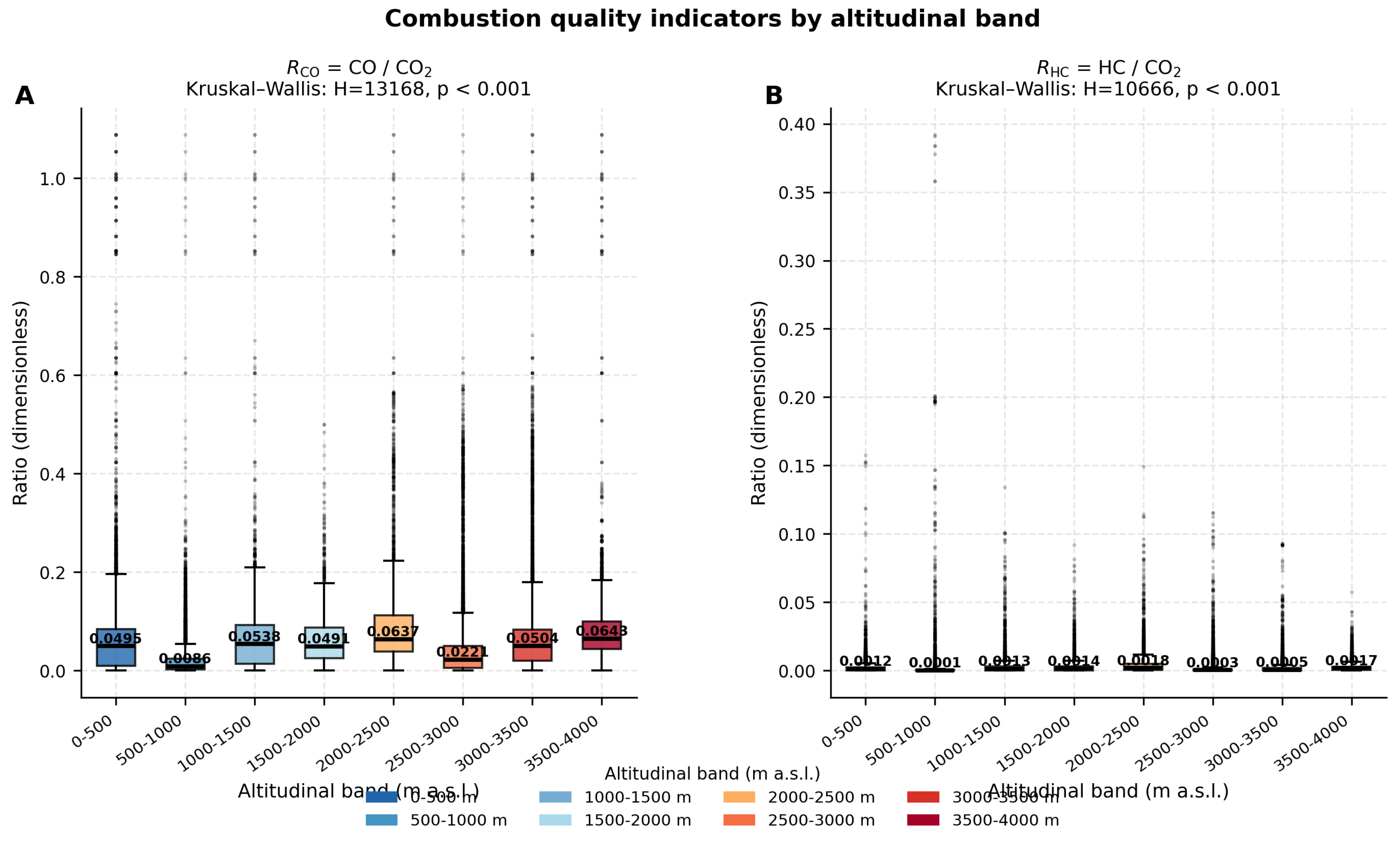
Figure 3.
Air-fuel ratio () along the altitudinal gradient. Panel A: median heatmap by altitudinal band and K-Means cluster (values below 1.0 indicate rich mixture; above 1.0 lean mixture). Panel B: distribution by band; dashed line marks the stoichiometric condition ().
Figure 3.
Air-fuel ratio () along the altitudinal gradient. Panel A: median heatmap by altitudinal band and K-Means cluster (values below 1.0 indicate rich mixture; above 1.0 lean mixture). Panel B: distribution by band; dashed line marks the stoichiometric condition ().
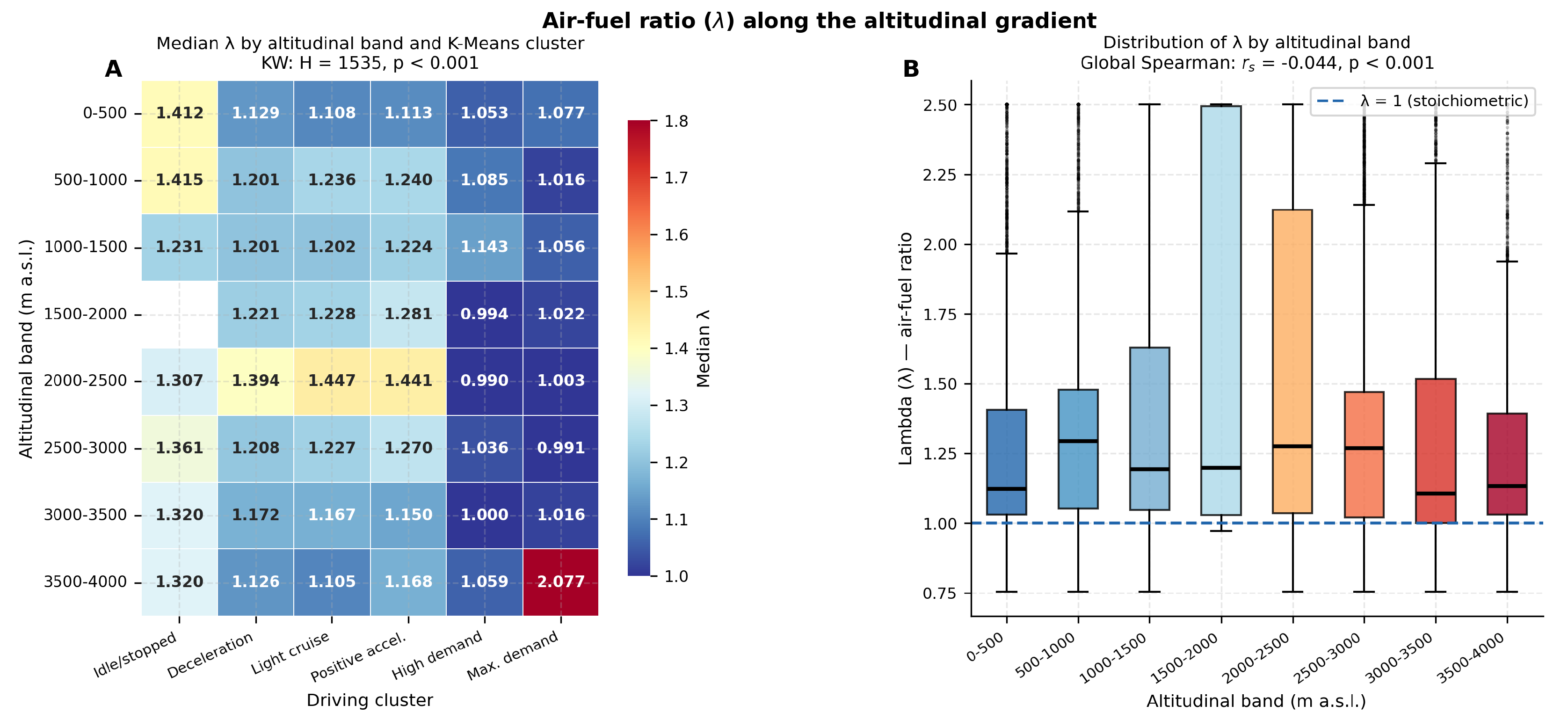
Figure 4.
Median altitudinal trends of exhaust gas concentrations. Panel A: CO (%vol); Panel B: HC (ppm); Panel C: NO (ppm); Panel D: CO2 (%vol). Shaded bands represent the IQR. Coloured markers follow the altitudinal gradient. Red shading highlights the band with the maximum value.
Figure 4.
Median altitudinal trends of exhaust gas concentrations. Panel A: CO (%vol); Panel B: HC (ppm); Panel C: NO (ppm); Panel D: CO2 (%vol). Shaded bands represent the IQR. Coloured markers follow the altitudinal gradient. Red shading highlights the band with the maximum value.
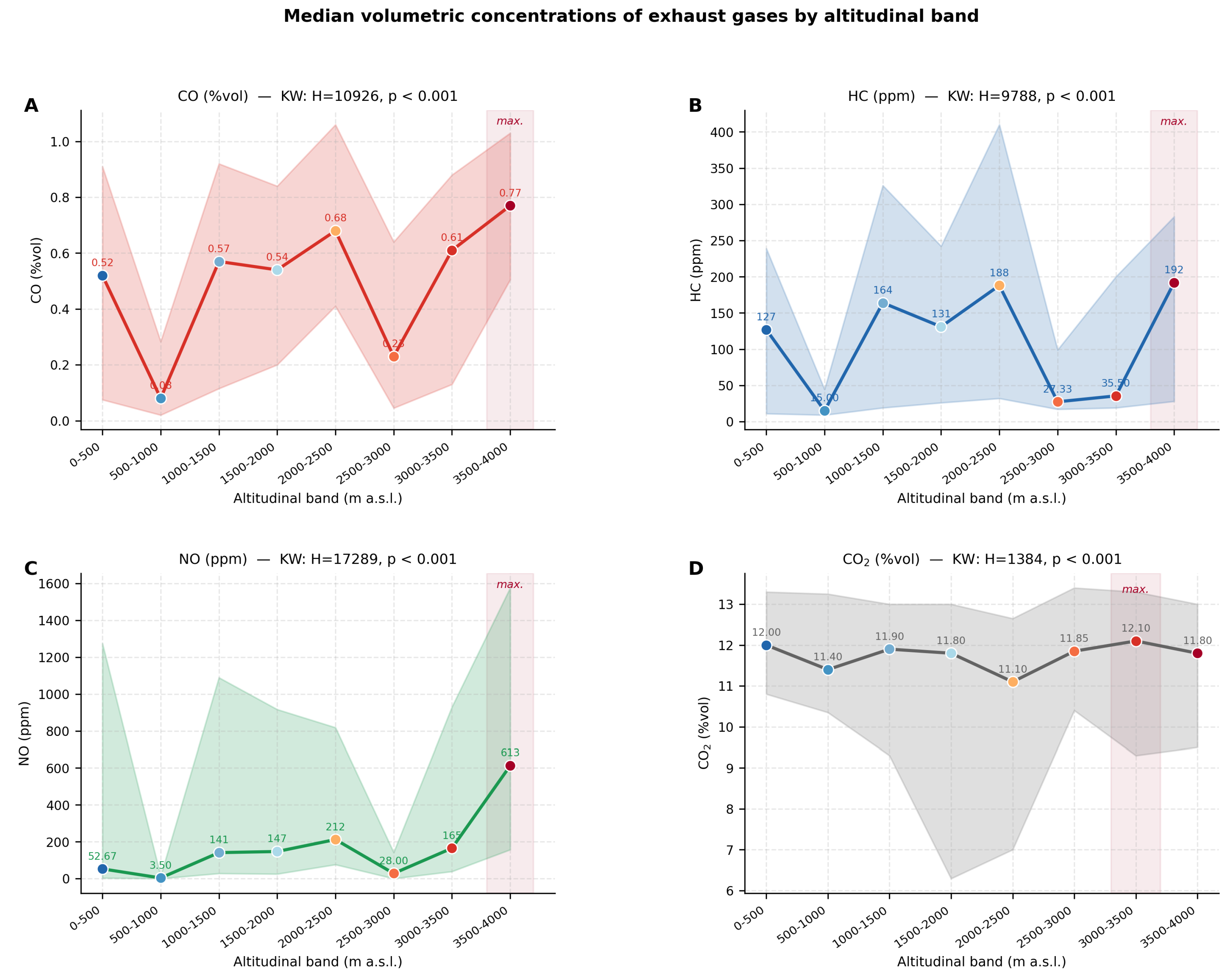
Figure 6.
Emission factors of CO (panel A), HC (panel B) and NO (panel C) in g/km by altitudinal band and K-Means driving cluster. Each coloured line represents a cluster median; the dashed black line shows the global median; shaded area shows the global IQR.
Figure 6.
Emission factors of CO (panel A), HC (panel B) and NO (panel C) in g/km by altitudinal band and K-Means driving cluster. Each coloured line represents a cluster median; the dashed black line shows the global median; shaded area shows the global IQR.
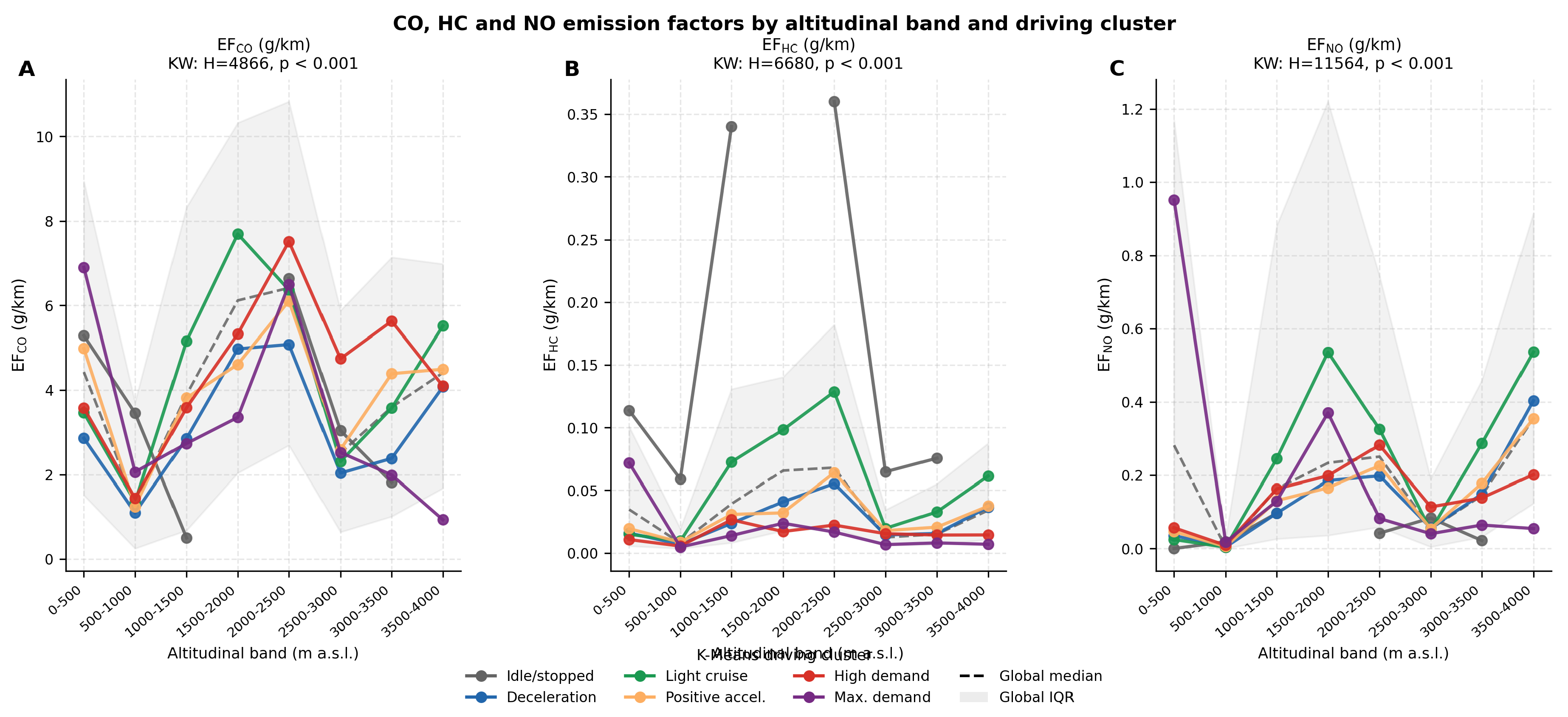

Table 1.
Main characteristics of the test vehicle fleet.
| ID | Fuel | Displacement (cm3) | Euro | Fuel mgmt. | Year | n (records) |
|---|---|---|---|---|---|---|
| V01 | Gasoline | 1400 | 2 | MPFI | 2010 | 8,742 |
| V02 | Gasoline | 1600 | 3 | MPFI | 2012 | 11,318 |
| V03 | Gasoline | 1800 | 3 | MPFI | 2013 | 9,215 |
| V04 | Gasoline | 1600 | 4 | MPFI | 2015 | 10,481 |
| V05 | Gasoline | 2000 | 4 | MPFI | 2016 | 9,876 |
| V06 | Gasoline | 1000 | 4 | MPFI | 2017 | 8,954 |
| V07 | Gasoline | 2000 | 5 | MPFI | 2019 | 11,632 |
| V08 | Gasoline | 2500 | 5 | MPFI | 2020 | 10,287 |
| V09 | Gasoline | 1800 | 5 | MPFI | 2022 | 9,143 |
| V10 | Gasoline | 1600 | 5 | MPFI | 2023 | 10,385 |
| Total | 100,033 | |||||
| MPFI: Multi-point fuel injection. | ||||||
Table 2.
Technical specifications of the Brain Bee AGS-688 analyser.
| Channel | Range | Resolution | Response time | Principle |
|---|---|---|---|---|
| CO | 0–9.99 % vol | 0.01 % vol | <10 s | NDIR |
| CO2 | 0–19.9 % vol | 0.10 % vol | <10 s | NDIR |
| HC | 0–9999 ppmvol | 1 ppmvol | <10 s | NDIR |
| NO | 0–5000 ppmvol | 1 ppmvol | <60 s | Electrochemical |
| NDIR: Non-dispersive infrared. Pressure compensation: 85.0–106.0 kPa. | ||||
Table 3.
Altitudinal bands with ISA atmospheric pressure and air density.
| Band | Altitude (m a.s.l.) | Pressure (kPa) | () |
|---|---|---|---|
| B1 | 0–500 | 101.3–95.5 | 1.225–1.167 |
| B2 | 500–1000 | 95.5–89.9 | 1.167–1.112 |
| B3 | 1000–1500 | 89.9–84.6 | 1.112–1.058 |
| B4 | 1500–2000 | 84.6–79.5 | 1.058–1.007 |
| B5 | 2000–2500 | 79.5–74.7 | 1.007–0.957 |
| B6 | 2500–3000 | 74.7–70.1 | 0.957–0.909 |
| B7 | 3000–3500 | 70.1–65.8 | 0.909–0.863 |
| B8 | 3500–4000 | 65.8–61.7 | 0.863–0.819 |
Table 4.
Record distribution by altitudinal band.
| Altitudinal band | Records (n) | % |
|---|---|---|
| 0–500 m | 21,882 | 23.2 |
| 500–1000 m | 14,188 | 15.1 |
| 1000–1500 m | 5,729 | 6.1 |
| 1500–2000 m | 2,316 | 2.5 |
| 2000–2500 m | 4,081 | 4.3 |
| 2500–3000 m | 22,834 | 24.2 |
| 3000–3500 m | 16,327 | 17.3 |
| 3500–4000 m | 6,906 | 7.3 |
| Total | 94,263 | 100.0 |
Table 5.
Medians (P25–P75) of combustion quality indicators by altitudinal band.
| Band | = CO/CO2 | = HC/CO2 | ||
|---|---|---|---|---|
| Median | P25–P75 | Median | P25–P75 | |
| 0–500 m | 0.0495 | 0.0098–0.0842 | 0.0012 | 0.0001–0.0021 |
| 500–1000 m | 0.0086 | 0.0027–0.0235 | 0.0001 | 0.0001–0.0005 |
| 1000–1500 m | 0.0538 | 0.0131–0.0919 | 0.0013 | 0.0002–0.0029 |
| 1500–2000 m | 0.0491 | 0.0253–0.0868 | 0.0014 | 0.0002–0.0031 |
| 2000–2500 m | 0.0637 | 0.0382–0.1123 | 0.0018 | 0.0006–0.0050 |
| 2500–3000 m | 0.0221 | 0.0052–0.0500 | 0.0003 | 0.0002–0.0010 |
| 3000–3500 m | 0.0504 | 0.0194–0.0835 | 0.0005 | 0.0002–0.0017 |
| 3500–4000 m | 0.0643 | 0.0440–0.1000 | 0.0017 | 0.0003–0.0027 |
| KW H | 13167.90*** | 10665.80*** | ||
| *** . | ||||
Table 6.
Median volumetric concentrations by altitudinal band. All Kruskal–Wallis contrasts significant ().
Table 6.
Median volumetric concentrations by altitudinal band. All Kruskal–Wallis contrasts significant ().
| Band | CO (%vol) | CO2 (%vol) | HC (ppm) | NO (ppm) |
|---|---|---|---|---|
| 0–500 m | 0.52 | 12.00 | 127.0 | 52.7 |
| 500–1000 m | 0.08 | 11.40 | 15.0 | 3.5 |
| 1000–1500 m | 0.57 | 11.90 | 164.0 | 141.0 |
| 1500–2000 m | 0.54 | 11.80 | 131.0 | 147.0 |
| 2000–2500 m | 0.68 | 11.10 | 188.0 | 212.0 |
| 2500–3000 m | 0.23 | 11.85 | 27.3 | 28.0 |
| 3000–3500 m | 0.61 | 12.10 | 35.5 | 165.0 |
| 3500–4000 m | 0.77 | 11.80 | 192.0 | 613.0 |
| KW H | 10926*** | 1384*** | 9788*** | 17289*** |
| *** . | ||||
Table 7.
Median emission factors (g/km) and fuel consumption (L/100 km) by altitudinal band.
| Band | EFCO | EFHC | EFNO | EFCO2 | Fuel cons. |
|---|---|---|---|---|---|
| (g/km) | (g/km) | (g/km) | (g/km) | (L/100 km) | |
| 0–500 m | 4.43 | 0.035 | 0.28 | 181.1 | 8.58 |
| 500–1000 m | 1.32 | 0.008 | 0.01 | 227.9 | 10.01 |
| 1000–1500 m | 3.89 | 0.039 | 0.16 | 147.6 | 7.97 |
| 1500–2000 m | 6.12 | 0.066 | 0.23 | 198.2 | 11.56 |
| 2000–2500 m | 6.42 | 0.068 | 0.25 | 143.1 | 8.83 |
| 2500–3000 m | 2.51 | 0.012 | 0.05 | 146.4 | 8.45 |
| 3000–3500 m | 3.60 | 0.015 | 0.14 | 125.4 | 8.16 |
| 3500–4000 m | 4.41 | 0.034 | 0.36 | 112.7 | 8.43 |
Disclaimer/Publisher’s Note: The statements, opinions and data contained in all publications are solely those of the individual author(s) and contributor(s) and not of MDPI and/or the editor(s). MDPI and/or the editor(s) disclaim responsibility for any injury to people or property resulting from any ideas, methods, instructions or products referred to in the content. |
© 2026 by the authors. Licensee MDPI, Basel, Switzerland. This article is an open access article distributed under the terms and conditions of the Creative Commons Attribution (CC BY) license (http://creativecommons.org/licenses/by/4.0/).
Copyright: This open access article is published under a Creative Commons CC BY 4.0 license, which permit the free download, distribution, and reuse, provided that the author and preprint are cited in any reuse.