

Submitted:
29 June 2026
Posted:
30 June 2026
You are already at the latest version
Abstract
An exchangeable pair-indexed Hawkes model for the collision statistics of a dilute hard-sphere gas is introduced. The event types are given by unordered particle pairs. It is proved that the integrated kernel belongs to the Johnson association scheme and that it has exactly three symmetry modes: a global mode, a tagged-particle mode and a cycle mode. The scalar aggregation of the total collision count is obtained, and the clock scaling induced by the kinetic collision frequency is identified. A cumulant obstruction is then proved: for every stationary positive multitype Hawkes process with a Poisson-cluster representation, each projected count has third long-time cumulant at least as large as its second long-time cumulant. The Sonine benchmark of Visco, van Wijland and Trizac for tagged hard-sphere collisions in dimension three has second-to-first cumulant ratio 363/320 and third-to-first cumulant ratio 1129729/1024000, so the third cumulant rate is smaller than the second. This comparison indicates that the positive Hawkes model yields a reference model, whereas the hard-sphere collision statistics require inhibition or latent kinetic states.
Keywords:
Hawkes process
; hard-sphere gas
; collision statistics
; Boltzmann–Grad limit
; Poisson cluster process
; inhibition
1. Introduction
Hawkes [1] introduced self-exciting point processes in order to describe event sequences for which previous events facilitate the occurrence of future events. Hawkes and Oakes [2] showed that the classical positive linear Hawkes process may be represented as a Poisson cluster process. This cluster representation is one of the reasons why Hawkes processes admit a detailed asymptotic theory, including limit theorems for multivariate processes [3] and large deviations for Poisson cluster processes [4]. Related renewal versions and cluster constructions have been studied in [5,6].
In this paper, the Hawkes framework is used to examine collision statistics in a gas of hard spheres. Since a collision record is a point process, this is a natural formulation. Nevertheless, the physical model is not an arbitrary sequence of events. Let , let , and consider identical hard spheres of diameter in a periodic box. Between collision times, the positions satisfy , while at a binary contact , with , the velocities are transformed by
This rule preserves total momentum and kinetic energy. If denotes the number of collisions between particles i and j before time t, then the natural event space is not the physical coordinate set , but rather
The total collision count is
The dilute hard-sphere gas is also a kinetic object. In dimension three, if denotes the collision cross-section, V denotes the volume, m denotes the mass, T denotes the temperature and denotes Boltzmann’s constant, then two independent Maxwellian particles have mean relative speed
It follows that one fixed unordered pair has dilute collision rate
and a tagged particle has collision frequency approximately
In the Boltzmann–Grad regime [7,8,9], the diameter tends to zero while the mean collision frequency remains of order one. Hence temperature and density determine the dimensional clock, while dimensionless correlation parameters have to be inferred from normalized collision statistics.
The purpose of this paper is to establish what is obtained from the positive Hawkes description and where this description ceases to match hard-sphere statistics. First, the exchangeable pair-Hawkes process is constructed and it is proved that its integrated kernel has three modes. The global mode gives the scalar Hawkes model for the total collision count. The tagged-particle mode controls fluctuations of . The cycle mode controls contrasts which are not visible from a scalar count. Then a cumulant obstruction for positive Hawkes models is proved: every projected count of such a process has at the level of long-time cumulant rates. This is incompatible with the three-dimensional hard-sphere Sonine benchmark of Visco, van Wijland and Trizac [10], for which
The discrepancy is not caused by using too few Hawkes dimensions. It is a consequence of the independent nonnegative branching mechanism itself.
2. The Physical and Point-Process Models
The basic objects used throughout the paper are now introduced.
Definition 1.
The hard-sphere collision process is the family
where denotes the number of binary elastic collisions of the pair e up to time t. The total and tagged counts are respectively
If impulses or velocities are retained, this becomes a marked point process. In the sequel, the Hawkes model is applied only to the unmarked collision times and pair labels.
Definition 2.
Let be locally integrable kernels and let . The exchangeable pair-Hawkes process is defined as the multivariate point process whose conditional intensities are given by
When the kernels are nonnegative, this gives a positive linear Hawkes process. When signed kernels are allowed, the expression in the right hand side is only a pre-intensity unless a nonnegative link function is imposed.
The three kernels have the following interpretation. The term corresponds to same-pair recollision effects, corresponds to propagation through one outgoing particle, and corresponds to collective effects between disjoint pairs. For a dilute gas, these effects need not all be positive. In particular, immediately after a collision the same two particles are separating, and a short-time same-pair effect is expected to be inhibitory. This observation is not used in the positive Hawkes theorems below; it only indicates the physical limitation of the positive model.
Let
The integrated kernel matrix is
3. The Three Symmetry Modes
Let , and identify with functions on . Let B be the unoriented incidence matrix,
Define
Theorem 1
(Three-mode decomposition). For ,
with
The matrix K in acts on these subspaces by the eigenvalues
and
Proof.
The dimensions are obtained from the incidence matrix. If , then for all , and since , this implies . Thus , and . Moreover, the map is injective on , so . The displayed dimensions add to M, and the three subspaces have trivial intersections; hence they form a direct sum.
For , each edge has one same edge, edges sharing one endpoint, and disjoint edges. This proves .
Let with . For , . The sum of over all f sharing one endpoint with e is
The sum over all f disjoint from e is
Therefore , which proves the asserted particle eigenvalue.
Finally let . Then the sum of over all edges incident to a fixed vertex is zero. For , the sum over edges sharing one endpoint with e is . Since , the sum over edges disjoint from e is . Hence , which is . This proves the theorem. □
The global subspace corresponds to total activity. The particle subspace corresponds to tagged-particle imbalances. The cycle subspace corresponds to partner-exchange contrasts such as
Corollary 1.
If the kernels in are nonnegative, the stationarity condition for the pair-Hawkes process is .
4. Scalar Aggregation and Kinetic Clock Scaling
The total collision count is the global projection of the pair process.
Proposition 1
(Scalar aggregation). For the pair-Hawkes process , the total conditional intensity satisfies
where
Then is a scalar Hawkes process whenever is a positive linear Hawkes process.
Proof.
Fix a previous event on . In the sum over all current edges e, this event contributes once through the same-edge kernel, times through the shared-edge kernel, and times through the disjoint-edge kernel. Summing over all previous events gives and , as required. □
Proposition 2
(Kinetic clock scaling). Suppose that a hard-sphere gas at temperature T is transformed to by multiplying all velocities by , while the geometry is unchanged. If the collision count admits a Hawkes representation with baseline and kernel , then the time-rescaled process at temperature has parameters
Then
Proof.
Under the velocity scaling , free-flight times are divided by c, while the sequence of collision labels is unchanged. Therefore the new count satisfies . The conditional intensity of a time-rescaled point process is multiplied by c: . Substitution of the Hawkes form gives , and the change of variables gives . □
Thus temperature changes the dimensional clock but not the integrated gains. For a fixed pair in dimension three,
and for a positive pair-Hawkes model in stationarity,
The baseline rate is therefore read as the exogenous kinetic clock
5. Macroscopic Hawkes Limits
Let denote the orthogonal projections onto . For the stationary positive pair-Hawkes process, the multivariate Hawkes functional central limit theorem [3] gives a Gaussian limit whose covariance rate is
This formula is obtained by diagonalizing the standard covariance matrix in the three eigenspaces of K.
Proposition 3
(Mode variances). Assume the hypotheses of the multivariate Hawkes central limit theorem and let r be the common stationary rate of each edge. Then the total count has the long-window Fano factor
For a tagged particle,
For four distinct particles,
satisfies
Proof.
The vector corresponding to is , which belongs to . Since , gives
and follows because .
The tagged count corresponds to the i-th row of the incidence matrix. Its projection on has squared norm
The remaining component lies in , and its squared norm is
Substitution in and division by gives .
The vector of has coefficients on the four displayed edges and zero elsewhere. Its incidence sums vanish at every vertex. Hence it belongs to , and its squared norm is 4. Formula follows from , which completes the proof. □
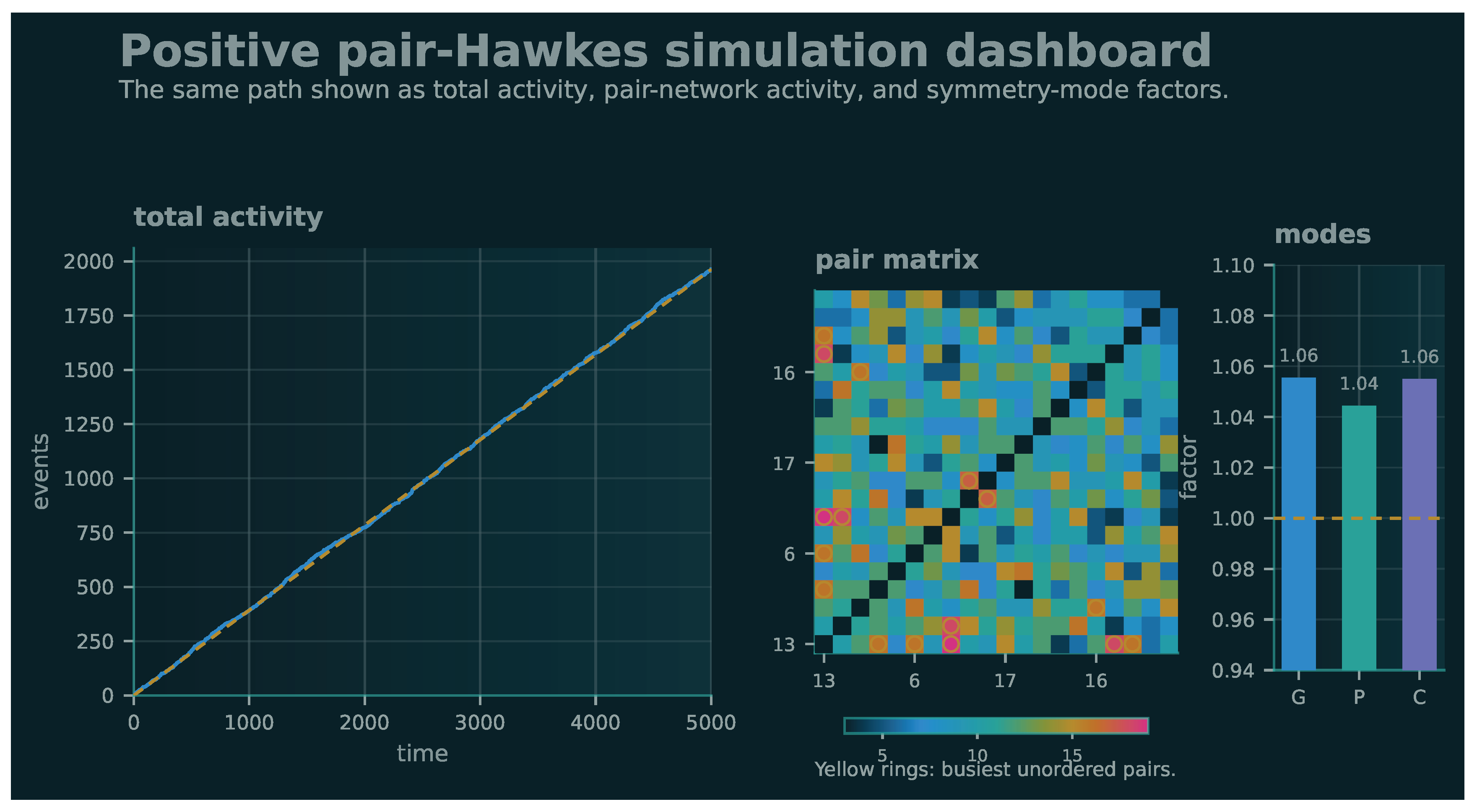
The preceding mode formulas and the pair-indexed structure are illustrated in Figure 1 by a positive pair-Hawkes simulation generated from the accompanying Python script. The left panel is the cumulative total count , and therefore displays the global projection . The middle panel is the matrix of unordered pair counts after particles have been ranked by their tagged totals . It shows that the basic event types are collision pairs, rather than particles, and that the particle mode is visible through heterogeneity of the row and column sums. The right panel reports the finite-window variance factors obtained by projecting the simulated binned counts on the global, particle and cycle subspaces . The simulation is only a positive Hawkes reference model; no hard-sphere conclusion is drawn from it.
Figure 1.
A simulated positive pair-Hawkes trajectory. Left: the cumulative total collision count , with a dashed line showing the empirical mean rate. Middle: unordered pair counts , displayed after ordering particles by tagged activity; yellow rings mark the busiest pairs. Right: finite-window variance factors for the global G, particle P and cycle C symmetry modes. The simulation uses , , bin width , and fixed seed 7.
Figure 1.
A simulated positive pair-Hawkes trajectory. Left: the cumulative total collision count , with a dashed line showing the empirical mean rate. Middle: unordered pair counts , displayed after ordering particles by tagged activity; yellow rings mark the busiest pairs. Right: finite-window variance factors for the global G, particle P and cycle C symmetry modes. The simulation uses , , bin width , and fixed seed 7.
The Hawkes limit gives event-count means and Gaussian activity fluctuations. It does not give Maxwellian velocities, momentum conservation, energy conservation, the Boltzmann collision operator, or pressure. For pressure one needs impulse marks. If denotes the normal impulse of the k-th collision, a virial pressure observable has the form
whereas an unmarked Hawkes model only describes the activity clock.
6. A Positive-Hawkes Cumulant Obstruction
For a count , write
whenever the limit exists.
Theorem 2
(Projected-count cumulant obstruction). Let N be a stationary multitype linear Hawkes process with nonnegative kernels. Assume that its integrated kernel has spectral radius less than one and that the kernels have finite first time moments. Let A be a subset of event types and set
If the third cluster moment of is finite, then the long-time cumulant rates satisfy
More generally, for every for which the corresponding cluster moments are finite.
Proof.
By the nonnegative-kernel assumptions and the spectral-radius condition, the process has the Hawkes–Oakes Poisson-cluster representation. Immigrants of type f arrive as independent Poisson processes with rates . Let be the number of points in the projection A generated by one cluster rooted at type f. The finite first time moment implies that boundary clusters contribute to cumulants on . Therefore the long-time cumulant rate of order n is the compound-Poisson cluster moment
Since is a nonnegative integer,
for every . Multiplying by , summing over f, and using gives the assertion. □
This theorem applies to scalar Hawkes processes, to the pair-Hawkes process above, and to every projection of every positive multitype Hawkes process. It is therefore a structural property of nonnegative branching, not a consequence of a low-dimensional parametrization.
7. Comparison with Hard-Sphere Cumulants
Visco, van Wijland and Trizac [10] studied the number of collisions of a tagged particle in a dilute equilibrium hard-sphere gas. Their tilted linear-Boltzmann analysis gives, in the Sonine approximation,
and
For , these formulas give
and
Hence , which contradicts .
The comparison is conditional in the following precise sense. The Hawkes obstruction theorem is exact. The hard-sphere input in – is the cited Sonine benchmark, supported in [10] by molecular dynamics, DSMC and population dynamics computations. Therefore the rigorous conclusion is that no positive Hawkes or positive Poisson-cluster model can have those benchmark cumulant rates as an exact projected-count limit.

Table 1.
Cumulant comparison from the generated output values.
| Quantity | Value | Consequence |
|---|---|---|
| Hard-sphere | overdispersed | |
| Hard-sphere | below | |
| Scalar Hawkes matching | fitted by variance | |
| Scalar Hawkes predicted | too large |
Figure 2.
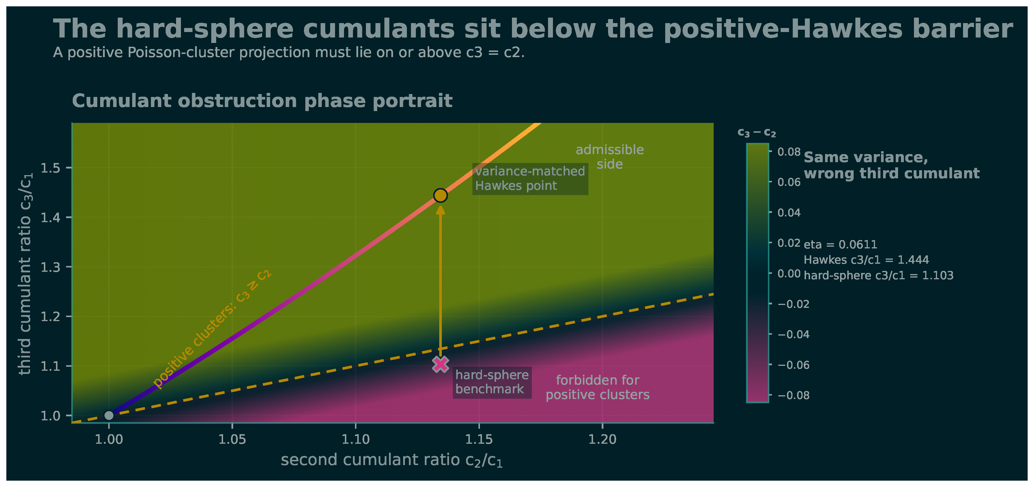
Cumulant obstruction map. The positive Poisson-cluster inequality defines the admissible side of the diagonal, while the three-dimensional hard-sphere Sonine benchmark lies below it. Matching the second cumulant ratio with a scalar positive Hawkes process moves vertically to a much larger third cumulant.
Figure 2.
Cumulant obstruction map. The positive Poisson-cluster inequality defines the admissible side of the diagonal, while the three-dimensional hard-sphere Sonine benchmark lies below it. Matching the second cumulant ratio with a scalar positive Hawkes process moves vertically to a much larger third cumulant.
For a scalar positive Hawkes process with branching ratio ,
Matching gives
The scalar Hawkes third cumulant is then
whereas the hard-sphere benchmark gives . The multitype positive pair-Hawkes model cannot remove this discrepancy for any projected count, since Theorem 6.1 applies before any symmetry reduction is made.
8. Inhibition and Latent Kinetic States
The preceding obstruction indicates the missing mechanisms. A tagged particle with velocity v has a collision hazard , and at a collision time velocities are sampled with the biased density
This gives apparent self-excitation, since a recent collision reveals that the tagged particle is likely to have a high collision rate. However, this memory is not additive branching memory. The next hazard is determined by the current kinetic state after the collision. A kinetic reduced generator for the tagged count has the tilted form
where is the velocity transition rate density of the linear Boltzmann description. The scaled cumulant generating function is the principal eigenvalue of this tilted kinetic operator.
A Hawkes-type extension may still be used if inhibition is allowed. For example, a clipped signed pair process is defined by
The expected signs are , a possibly biphasic , and a small in the dilute limit. Such a model lies outside the positive cluster class. This is consistent with the inhibitory Hawkes literature, where the classical cluster representation no longer applies and renewal or likelihood arguments have to be modified [12,13,14].
9. Conclusions
An exchangeable pair-Hawkes construction for collision activity has been obtained. Its integrated kernel has three symmetry modes, its total count is a scalar Hawkes process, and its clock scaling is compatible with the kinetic collision frequency. On the other hand, every positive Hawkes projection satisfies the cumulant inequality . The three-dimensional hard-sphere benchmark of Visco et al. [10] contradicts this inequality. Hence positive branching is not an exact model of hard-sphere collision statistics at the tagged-particle level.
Thus positive Hawkes processes give a mathematically controlled reference model whose obstruction indicates the missing physical structure: inhibition, conservation-law constraints, partner competition, recollision geometry and latent velocity states. A natural continuation is to estimate the three Hawkes modes from event-driven hard-sphere data and then to test, through cumulants and time-reversal diagnostics, which signed or latent-state extension remains compatible with kinetic theory.
Supplementary Materials
The following supporting information can be downloaded at the website of this paper posted on Preprints.org. The Python scripts and CSV files used to generate the numerical figure files and summary values are provided as Supplementary Materials.
Author Contributions
Conceptualization, L.I.H.R.; methodology, L.I.H.R.; software, L.I.H.R.; validation, L.I.H.R.; formal analysis, L.I.H.R.; investigation, L.I.H.R.; writing—original draft preparation, L.I.H.R.; writing—review and editing, L.I.H.R.; visualization, L.I.H.R.
Funding
This research received no external funding.
Institutional Review Board Statement
Not applicable.
Informed Consent Statement
Not applicable.
Data Availability Statement
The numerical values and figures in this manuscript were generated using the Python scripts provided as Supplementary Materials.
Acknowledgments
The author thanks the developers and maintainers of the open-source scientific Python and LATEX tools used to prepare the numerical figures and manuscript.
Conflicts of Interest
The author declares no conflicts of interest.
References
- Hawkes, A.G. Spectra of Some Self-Exciting and Mutually Exciting Point Processes. Biometrika 1971, 58, 83–90. [Google Scholar] [CrossRef]
- Hawkes, A.G.; Oakes, D. A Cluster Process Representation of a Self-Exciting Process. J. Appl. Probab. 1974, 11, 493–503. [Google Scholar] [CrossRef]
- Bacry, E.; Delattre, S.; Hoffmann, M.; Muzy, J.F. Some Limit Theorems for Hawkes Processes and Application to Financial Statistics. Stoch. Process. Their Appl. 2013, 123, 2475–2499. [Google Scholar] [CrossRef]
- Bordenave, C.; Torrisi, G.L. Large Deviations of Poisson Cluster Processes. Stoch. Model. 2007, 23, 593–625. [Google Scholar] [CrossRef]
- Hernandez Ruiz, L.I. Law of Large Numbers and Central Limit Theorem for Renewal Hawkes Processes. Stochastics 2025. [Google Scholar] [CrossRef]
- Hernandez Ruiz, L.I.; Yano, K. A Cluster Representation of the Renewal Hawkes Process. ALEA Lat. Am. J. Probab. Math. Stat. 2025, 22, 1347–1368. [Google Scholar] [CrossRef]
- Grad, H. Principles of the Kinetic Theory of Gases. In Handbuch der Physik; Springer, 1958; Vol. 12, pp. 205–294. [Google Scholar]
- Lanford, O.E. Time Evolution of Large Classical Systems. In Dynamical Systems, Theory and Applications; Springer, 1975; Vol. 38, Lecture Notes in Physics, pp. 1–111.
- Saffirio, C. Derivation of the Boltzmann Equation: Hard Spheres, Short-Range Potentials and Beyond. arXiv 2016, arXiv:1602.05355. [Google Scholar]
- Visco, P.; van Wijland, F.; Trizac, E. Collisional Statistics of the Hard-Sphere Gas. Phys. Rev. E 2008, 77, 041117. [Google Scholar] [CrossRef] [PubMed]
- Daley, D.J.; Vere-Jones, D. An Introduction to the Theory of Point Processes. Volume I, 2 ed.; Springer: New York, 2003. [Google Scholar]
- Bremaud, P.; Massoulie, L. Stability of Nonlinear Hawkes Processes. Ann. Probab. 1996, 24, 1563–1588. [Google Scholar] [CrossRef]
- Costa, M.; Graham, C.; Marsalle, L.; Tran, V.C. Renewal in Hawkes Processes with Self-Excitation and Inhibition. Adv. Appl. Probab. 2020, 52, 879–915. [Google Scholar] [CrossRef]
- Bonnet, A.; Martinez Herrera, M.; Sangnier, M. Maximum Likelihood Estimation for Hawkes Processes with Self-Excitation or Inhibition. arXiv 2021, arXiv:2103.05299. [Google Scholar]
Disclaimer/Publisher’s Note: The statements, opinions and data contained in all publications are solely those of the individual author(s) and contributor(s) and not of MDPI and/or the editor(s). MDPI and/or the editor(s) disclaim responsibility for any injury to people or property resulting from any ideas, methods, instructions or products referred to in the content. |
© 2026 by the authors. Licensee MDPI, Basel, Switzerland. This article is an open access article distributed under the terms and conditions of the Creative Commons Attribution (CC BY) license (http://creativecommons.org/licenses/by/4.0/).
Copyright: This open access article is published under a Creative Commons CC BY 4.0 license, which permit the free download, distribution, and reuse, provided that the author and preprint are cited in any reuse.


