

Submitted:
29 June 2026
Posted:
01 July 2026
You are already at the latest version
Abstract
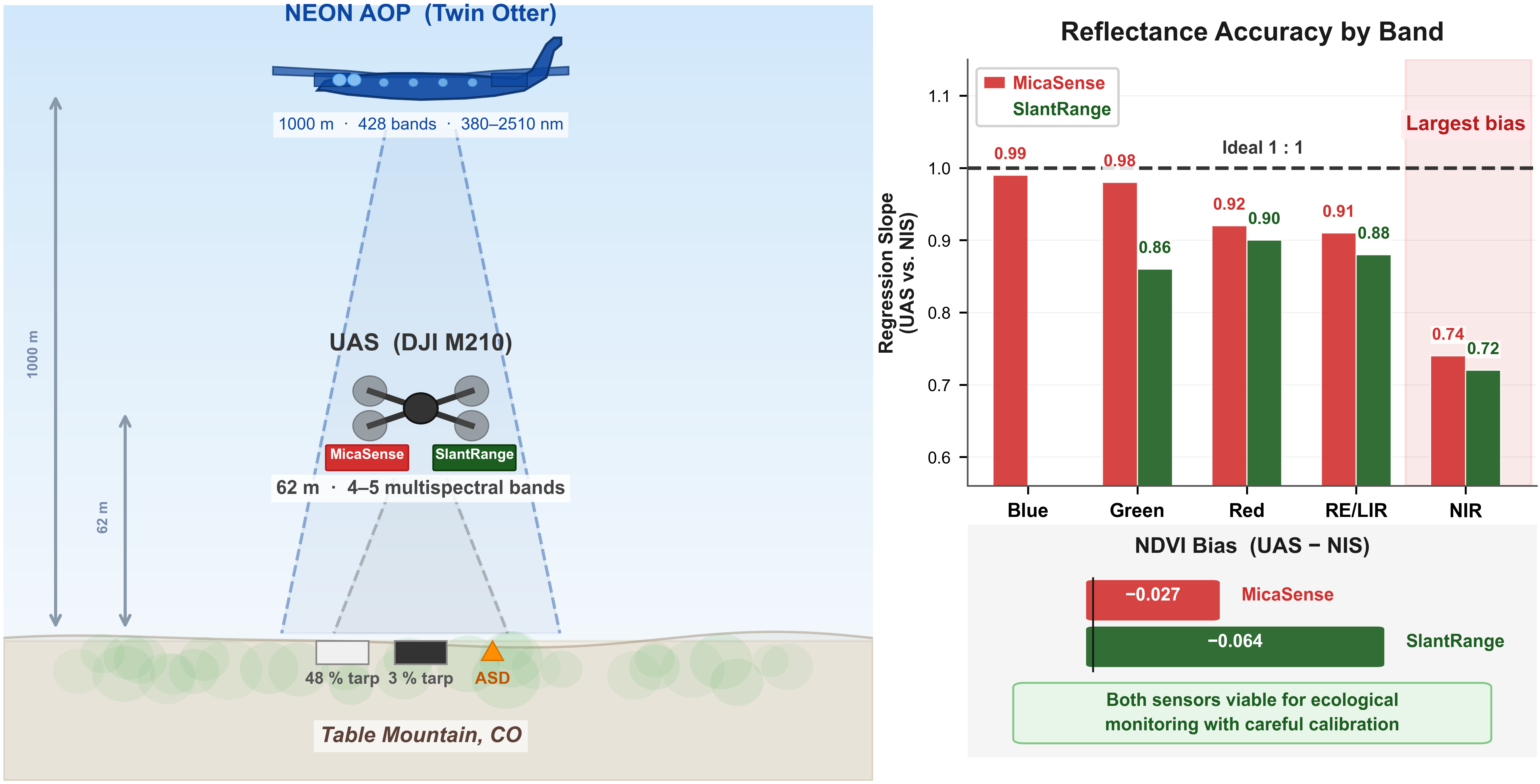
This study evaluates the accuracy and usability of two low-cost unmanned aerial system (UAS) multispectral sensors—MicaSense RedEdge and SlantRange 3p—by comparing their reflectance measurements and NDVI to those of the NEON Imaging Spectrometer (NIS), a well-calibrated airborne hyperspectral sensor. Field validation was conducted using calibrated reflectance tarps, and spectrally resampled NIS data served as a reference standard. Reflectance comparisons showed both sensors performed well across most land cover types but exhibited systematic biases that prevented statistical equivalence in most bands. The MicaSense sensor generally overestimated reflectance, while the SlantRange sensor underestimated it, particularly in the Green and NIR bands. These biases propa-gated into NDVI calculations, where both UAS sensors reported lower NDVI values than the NIS, with SlantRange showing a larger negative bias. Despite the lower NDVI values and artifacts, including BRDF effects at image edges and background noise over dark sur-faces, the results support the viability of UAS-based multispectral sensing for ecological applications requiring moderate to high accuracy. The study also highlights the critical importance of radiometric calibration and sensor-specific limitations in reflectance range. This comparison framework provides a foundation for broader cross-platform validation efforts and helps inform best practices for ecological remote sensing using low-cost UAS systems.
Keywords:
UAS
; multispectral
; hyperspectral
; NEON Imaging Spectrometer (NIS)
; radiometric calibration
; NDVI
1. Introduction
Lightweight imaging sensors paired with Uncrewed Aerial Vehicles (UAVs) have become ubiquitous research tools for earth observation over the last 20 years [1]. Coupling UAVs with lightweight remote sensing instruments–collectively termed Uncrewed Aerial Systems (UASs)–provides a low-cost and effective solution to collect imagery of landscapes that would otherwise be cost prohibitive with satellite or crewed aircraft platforms [2]. Due to the compact size and portability of low cost UAS, surveys benefit from flexibility in mission timing and location. However, UASs suffer from constraints on flight altitude and payload endurance. Within the United States, modern UASs are required to operate with a low altitude acquisition height (< 400 feet above ground level) due to FAA constraints. UAV platforms also typically have limited payload endurance, which is dependent on the type of platform, power source and payload capacity. The height and endurance limitations constrain surveys to a small geographic extent (~1 km2 per flight), and result in images with high spatial resolution. UASs have normalized the capture of EO (Earth Observing) images at extremely high spatial resolutions, often achieving sub-decimeter, or centimeter ground sample distances (GSD).
The high spatial and temporal resolution provide landscape characteristics, such as plant health and crop characteristics, at previously unavailable observational scales. Fine-scale spatial patterns that may have been previously indiscernible by the lower resolution imaging typical of sensors mounted on crewed aircraft and satellite platforms [3] are often revealed. In this capacity, UASs offer landscape ecologists a timely, cost-effective means of monitoring environmental phenomena at ecologically meaningful spatiotemporal resolutions, providing a powerful tool for ecological scaling studies [4]. UASs equipped with multispectral sensors have supported a multitude of agricultural applications, including mitigation of disease spread in rice fields [5], yield monitoring of fertilized peas and oats [6], high-resolution assessment of vine health in viticulture [7], and monitoring of nitrogen status in wheat to optimize fertilization practices [8,9]. However, ecological applications are increasingly being addressed as well, such as identifying sensitivities to environmental change in Antarctic moss beds [10] and precise and frequent mapping of rangeland characteristics [3]. Collectively, these studies and others underscore the value of UASs and offer a promising path forward for fine-scale localized environmental monitoring efforts. Large scale ecological networks, such as the National Ecological Observatory Network (NEON), may be particularly well suited to incorporate UASs due to the need for making repeated measurements across numerous large and dispersed research sites.
Imaging sensors typically mounted on UAS are lightweight and low cost. The already limited endurance of UAVs necessitates lightweight imaging payloads, as payload weight will further reduce platform endurance and introduce inefficiency to collection time. In addition, UAV platforms can be prone to erratic flight behavior in turbulent conditions or component failure that lead to accidents and damage to imaging sensors. Researchers are often hesitant to mount high grade / high-cost sensors on UAV platforms due to risk of accidents that render sensors unusable. Therefore, sensors typically used in UASs can suffer from design trade-offs that reduce accuracy to maintain weight and cost constraints. To understand the application space for low-cost UAS platforms, a rigorous analysis of typical sensor accuracy is required. While many studies have provided valuable insights into the implementation of lightweight and low-cost UAS sensors in agriculture and ecological research [2,3,4,5,6,7,8,9,10,11], quantitative assessments of the spectral accuracy of UAS sensors are limited. Matese et al. [11] compared Normalized Difference Vegetation Index (NDVI) data of an ASPIS (Advanced Spectroscopic Imaging System, a remote sensing system) sensor mounted on a crewed aircraft, and a Tetracam ADC Lite (Tetracam Inc., Chatsworth, CA, USA) sensor mounted on a UAS platform in two Italian vineyards. To our knowledge, the study by Matese et al. [11] study represents one of the few efforts to quantify the in situ spectral accuracy of a small lightweight imaging sensor over a broad geographic extent. Breni et al. [12] also covered a broad geographic extent with a rigorously calibrated sensor traceable to reference standards, however, did not provide independent in-situ validation measurements. Shrestha et al. [13] performed an in-situ accuracy assessment of radiometric calibration and reflectance retrieval of two UAS mounted sensors, a Headwall Nano-Hyperspec and MicaSense RedEdge-MX Dual Camera Imaging System. This study provided accuracy assessments over a variety of in-situ targets, each with limited spatial extent. Shrestha et al. [13] intended to also provide an accuracy assessment over a broader spatial extent through comparisons of temporally coincident satellite imagery; however, poor weather precluded this analysis. Despite these challenges, the target comparisons in Shrestha et al. [13] provide valuable insight into the accuracy of UAS mounted sensors at specific targets. To date, literature remains sparse on in-situ absolute spectral accuracy of UASs relative to traceable reference standards.
The objective of this study is to assess the spectral accuracy of two commercial low-cost and lightweight multispectral cameras mounted on a small UAV by conducting an in situ vicarious comparison with known reflectance targets coupled with high spectral accuracy measurements obtained via an imaging spectrometer mounted in the NEON Airborne Observation Platform (AOP). As demonstrated by Shrestha et al. [13], validation tarps allow a high-fidelity absolute validation at a unique point within the survey area. While the AOP allows for accuracy analysis across the entire extent and variety of targets of the UAS survey. This is an important first step in building a validation framework for potential synergistic UAS remote sensing campaigns to assess the suitability for different application areas and exploring interoperability with alternative data sources. We fully investigate the performance of each individual band collected by the multispectral cameras and also perform comparisons with NDVI data –a common vegetation index used to quantify plant health and vegetation density. Although we cannot definitively provide recommendations on whether UASs meet the needs of particular application areas, readers can assess our results to determine whether a UAS based platform meets their accuracy needs.
2. Materials and Methods
2.1. Study Site
Data collections were conducted at Table Mountain, north of Boulder, CO, USA (Figure 1). Table Mountain is used for annual NEON AOP calibration flights and the UAS data collection was conducted coincidentally with an annual operational NEON AOP calibration flight. In addition to its proximity to NEON Headquarters (Boulder, CO, USA), Table Mountain offers three advantages as a study site for conducting the proposed comparison between the UAS mounted sensors and the NEON AOP: 1) the vegetated portion of the landscape is homogeneous, which minimizes the uncertainty in comparisons due to slight spatial mismatches between the UAS and AOP data; 2) it is relatively flat, which reduces uncertainty in reflectance retrievals due to topographic variation; 3) it houses a permanently mounted aerosol monitoring sensor (part of AERONET, https://aeronet.gsfc.nasa.gov/), which allows for accurate characterization of aerosol optical depth at the time of data acquisition, improving reflectance retrieval accuracy of the imaging spectrometer. The Table Mountain data collection area included two intersecting gravel roads, vegetation, and deployed reference tarps.
2.2. Data Collection
2.2.1. Reference Tarps with Field Spectral Measurements
Two reference tarps, manufactured by Group 8 Technologies (https://www.group8tech.com/), were placed within the flight area observed by the NEON AOP and the UAS. The tarps are 10 m by 10 m in size and are coated with a specialized material with well-known spectral response in the visible through short-wave infrared (SWIR) portion of the electromagnetic spectrum. The two reference tarps represent end-member reflectance targets with one tarp reflecting ~48% of incoming energy and the other reflecting ~3% across all wavelengths of interest. The tarps are hereafter referred to as the ‘bright’ and ‘dark’ reference tarps, respectively.
Although the tarps are designed to have specific reflectance values across all wavelengths, the reflectance can vary slightly from the design value. Given the intention to assess the absolute spectral accuracy of the UAS mounted sensors, the tarps were also observed with an Analytical Spectral Device (ASD) field spectrometer during the airborne acquisitions to ensure spectral accuracy. The ASD provides highly accurate measurements of spectral reflectance at 1 nm intervals which serves a basis for comparing the UAS mounted sensors to a known reflectance target, as well as verifying the spectral accuracy of the imaging spectrometer to ensure its suitability as a validation source. Directly before and after ASD measurements were acquired over each reference tarp, the ASD also observed a calibrated Spectralon panel, which is used as a white reference to calibrate the ASD measurements.
2.2.2. National Ecological Observatory Network Airborne Observation Platform
The NEON imaging spectrometer (NIS) was developed at the Jet Propulsion Laboratory (JPL) and is a next-generation AVIRIS (Airborne Visible / Infrared Imaging Spectrometer) instrument. The NIS collects data in 428 spectral bands covering 380 to 2510 nm. Band centers are separated by ~5 nm [14] and the spectral response for individual bands is up to ~6 nm. The NIS operates in a push-broom configuration with a cross-track field of view (FOV) of ~36° and an instantaneous field-of-view (IFOV) of 1 mRad. The NIS undergoes an annual rigorous calibration process to ensure spectral and radiometric fidelity of the instrument.
The NEON AOP Table Mountain flight plan included three flight lines, which were flown in a south-north, east-west and north-south orientation, all at an altitude of 1000 m. The flight line placement captured the calibration tarps and the area observed by the UAS at the center of each NIS flightline. At a 1000 m altitude, the total flightline width is 628 m and with an IFOV of 1 mRAD the individual sensing elements of the spectrometer focal plane array will observe an area of ~1 m2. The NIS observes lines at 100 Hz and the aircraft travelled at ~50 m/s, which allows for an over-sampling of the terrain, as a single line of observations was collected approximately every 0.5 m. The NEON AOP includes a positioning and orientation system that includes a high accuracy GPS and inertial measurement unit allowing for high accuracy in aircraft position throughout the survey. Annual calibration flights determine the boresight angles of the imaging spectrometer, and coupled with the high accuracy positioning, can achieve a spatial accuracy of less than 1 m at the normal flying altitude of 1000 m.
2.2.3. Uncrewed Aerial System
The UAS mission captured images using two multispectral sensors: the MicaSense RedEdge M (MicaSense Inc., Seattle, WA) and the SlantRange 3p (SlantRange Inc., San Diego, CA), temporally coincident with an acquisition by the NEON AOP. The multispectral sensors capture images over the visible to near-infrared (NIR) spectral range, with the RedEdge being a 5-channel sensor and the SlantRange a 4-channel sensor (Table 1). Table 1 provides the band center wavelength and approximate width of the spectral response function for each band, however, precise spectral response functions for each multispectral band were provided by the manufacturers. Each multispectral sensor is accompanied by a downwelling light sensor (DLS) and a GPS antenna and receiver. Both the RedEdge and SlantRange use the DLS to correct reflectance for ambient light changes.
The sensors were mounted on a DJI Matrice 210 (hereafter referred to as ‘M210’ for the remainder of the manuscript; DJI Inc., Shenzhen, China). The M210 is a VTOL (vertical takeoff and landing) quadcopter powered by two 22.8 V rechargeable batteries and is equipped with two downward facing gimbals and one upward facing gimbal. Each camera was independently secured to the downward facing gimbals of the M210 at an ~8° offset from nadir (Figure 2a). Gimbals ensure camera stabilization while the UAS maneuvers in flight. The DLS and GPS units of the RedEdge sensor were secured to the upward facing gimbal of the M210, whereas the DLS and GPS of the SlantRange –a single piece of equipment– was attached to the bar of the M210’s field-of-view camera (Figure 2b). Prior to flight, all manufacturer recommended sensor-specific calibrations were performed.
Flight planning was conducted using Drone Deploy, a UAS flight planning and auto-pilot software (Drone Deploy, San Francisco, CA, USA). The flight area is depicted in Figure 3a and speed and flight altitude were set at 6 m/s and 62 m above ground level (AGL), respectively. The image overlap settings of the SlantRange 3p are provided as ‘sidelap’ (cross-track overlap) and ‘frontlap’ (along-track overlap), both set to 75%. This is the minimum recommended overlap of the RedEdge sensor [15]. The MicaSense flight planning application was used to determine the appropriate image capture rate (> 1.72 sec) for the desired overlap and flight altitude settings. The RedEdge sensor was then calibrated by positioning the UAS above the MicaSense Calibration Reflectance Panel (CRP), capturing two calibration images of the panel. This approach follows recommendations from MicaSense for flying in clear sky conditions, which notes to use the CRP for post-processing calibrations rather than relying solely on the DLS corrections [15]. The flight path of the UAS was programmed to perform a ‘lawnmower pattern’, consisting of parallel east-west lines within the flight area (Figure 3a).
Best practices dictate that flights should be conducted within ± 2 hours of local solar noon to mitigate solar angle variation [17]. Our UAS flight began at 11:56:58 (MST) and overlapped with solar noon (11:58:52 MST; see [18]). The 12-min flight ended at 12:09:10 (MST), was accompanied by light winds and sunny conditions (0% cloud cover) with visibility > 10 miles (see Figure 3b-c). The entire flight was auto-piloted by the Drone Deploy software and minimal manual flying was utilized except when realigning the UAS with the launch pad prior to landing.
2.3. Data Processing
2.3.1. National Ecological Observatory Network Imaging Spectrometer (NIS)
The NIS laboratory determined calibration parameters were used to transition raw observations to at-sensor radiance. The details of the application of calibration parameters to raw data to produce at-sensor radiance can be found in Gallery and Leisso, 2014 [19]. After determination of at-sensor radiance, each pixel is rigorously geo-referenced using a ray-tracing algorithm outlined in Kampe et al., 2016 [20] that intersects the observation vector with the high accuracy terrain model derived from an airborne lidar survey. The NEON AOP is prohibited from operating their lidar sensor over Table Mountain, so a publicly available lidar acquisition was used [22]. After ray-tracing, pixels are geo-located in a pseudo-random pattern that is dependent on flight conditions. To re-locate pixels to an even one-meter grid, a nearest neighbor resampling routine was employed.
At-sensor radiance is transitioned to surface reflectance using the ATCOR (Atmospheric and Topographic Correction) 4 commercial software package developed by ReSe Applications (https://www.rese-apps.com/). Details of the atmospheric correction algorithms can be found in Richter and Schlapfer, 2018 [23]. Although several parameters required for surface reflectance retrievals can be fine-tuned prior to executing ATCOR, experience has shown that results are primarily sensitive to the ‘Visibility’ parameter, which is related to the aerosol optical thickness (AOT). ATCOR can provide an estimate of this parameter based on information determined from dark dense vegetation in the scene (see Richter and Schlapfer, 2018 [23]). However, at the time of flight very little dark dense vegetation was available at the Table Mountain site, which would inhibit a reliable numerical estimate of the visibility parameter. A more accurate determination of the Visibility parameter can be obtained through direct measurement using a sun photometer. For the time of acquisition, sun photometer measurements from Table Mountain are available through Aeronet (https://aeronet.gsfc.nasa.gov/). ATCOR requires visibility calculated from AOT at 550 nm, however, Aeronet does not provide AOT at 550 nm. Therefore, AOT at 550 nm was calculated as:
where AC is the Angstrom coefficient (also provided by Aeronet) and 〖AOT〗_550 is the AOT at 500 nm. Following Wilson et al., 2015 [24], the visibility at 550 nm was calculated as:
Parameters supplied to ATCOR included visibility, a flag to turn on topographic correction, a flag to apply an adjacency correction, the limit of the adjacency correction (which was set to 10 m), a flag to correct for changes in the solar zenith angle, and the scene class which was set to ‘rural’. Output surface reflectance was produced at the input spectral resolution of 5 nm and the input spatial resolution of 1 m.
The spectral resolution of the multispectral UAS sensors is coarse compared to that of the NIS. To allow a direct comparison between the MicaSense and SlantRange sensors and the NIS, the NIS surface reflectance was spectrally resampled to the system spectral response curves for the respective multispectral sensors’ bands. Both the manufacturers of the SlantRange and MicaSense provided the spectral response curves for each band of the sensor, although we note that the provided curves were generalized curves associated with the sensor product line and were not specific to a unique sensor. A spectral convolution was applied to the NIS data to produce new bands that corresponded to the spectral response for each band of the MicaSense and SlantRange sensors. The resampled NIS bands, based on the spectral response of the UAS sensors, were calculated as:
where is the result of the NIS data resampled to the UAS band, is the observed value of reflectance from the NIS at band , and is the convolution operator for band j of the UAS sensor with band k of the NIS, which can be defined as:
where is the value for the spectral response function for the NIS at wavelength , and is the spectral response function for the UAS sensor. To numerically determine values of , an interval of 1 nm was used.
2.3.2. Analytical Spectral Device Field Spectrometer
Data collected with the ASD field spectrometer was transitioned from raw measurements to reflectance using in-house NEON algorithms. Comparisons of the NIS resampled data, as well as data from the SlantRange and MicaSense sensors, to the field spectrometer measurements required a spectral resampling from the 1 nm field spectrometer reflectance curves to the spectral response of each band of the SlantRange and MicaSense sensors. Since spectral response functions of the field spectrometer were not available from ASD, they were assumed to be a uniform distribution at each 1 nm band. This simplifies the spectral resampling calculations as:
where is the wavelength, is the value of the spectral response function of the UAS sensor for a particular band at a given wavelength, is the observed reflectance from the ASD at a given wavelength, and is a simulation of what the ASD would have observed for a particular band of the UAS sensor. These calculations were performed at a 1 nm interval to match the precision of the ASD observations. Since the spectral resolution of the field spectrometer was much finer (1 nm) than the MicaSense and SlantRange sensors, we do not believe that simplifying the resampling relationship by assuming a uniform distribution of spectral response functions of the ASD has a significant effect on the final reflectance values of .
2.3.3. SlantRange
Raw data files from the SlantRange sensor were pre-processed using the proprietary Slantview software (SlantRange Inc., San Diego, CA) to convert raw images to reflectance and perform image calibration and alignment. Orthomosaic images were made using the DroneDeploy software (https://www.dronedeploy.com), a cloud-based image processing software application. Because the DroneDeploy software is limited to images of three bands or less, SlantRange orthomosaics were generated over two executions of the DroneDeploy software. In the first execution, the Green, Red, and LIR (Leading Infrared) bands were processed, and the Green, Red, and NIR bands were processed in the second execution. This routine resulted in two final orthomosaics for comparison with the NIS, however the Green and Red bands were redundant and required access from only one of the orthomosaic images. Final SlantRange reflectance values were scaled between 0 and 255 to maintain the maximum amount of radiometric resolution in an 8-bit image. All SlantRange reflectance values were normalized by dividing by 255 prior to comparison with reflectance traps or the NIS.
2.3.4. MicaSense
The raw data files output by the MicaSense RedEdge multispectral sensor are in GeoTIFF format; however, the individual bands are provided as individual TIFF files. This results in 5 total TIFF files per capture. Images were processed using Agisoft Metashape Pro (Agisoft LLC, St. Petersburg, Russia). The data were processed following instructions provided by Agisoft that were specific to MicaSense RedEdge cameras. The photos were ingested to Metashape along with the two calibration images and the reflectance panel calibration coefficients. The photos were then geo-referenced and the individual band cameras optimized using an Agisoft Metashape Pro built-in functionality that identifies ‘tie points’ between images to create a model surface for aligning photos. Subsequently, the calibrated and aligned images were used to build an orthomosaic image. The resulting orthomosaic was output as a signed 16bit GeoTIFF with normalized reflectance values by dividing each band by 32,768 which is the maximum scale factor for a signed 16-bit integer.
2.3.3. Spatial Resampling
The spatial resolutions of the multispectral sensors are dependent upon the flight altitude specified during mission planning. The specified ground sampling distance (GSD) at a 62 m flight altitude is 2.48 cm for the SlantRange and 4.31 cm for the MicaSense. Comparatively, the NIS provides post-processed data at a 1 m resolution. To compare the output of these remote sensing platforms, the UAS multispectral sensor data were resampled to 1 m resolution to match the NIS data. The resampling involved defining the extent to crop out aligned areas of the UAS and NIS mosaics, ensuring that multispectral data were aggregated over the same 1 m areas sampled by the NIS. For each 1 m NIS pixel, all pixels from the higher resolution UAS acquisitions whose centers were located within the NIS pixel were included in an average. Given the pixel sizes in the UAS images were not perfectly divisible within the 1 m NIS pixel, this could result in some pixels from the UAS acquisitions with partial overlap in adjacent NIS pixels, however, this artifact is believed to have negligible influence to the final mean given the much smaller size of the UAS pixels.
A small spatial mismatch was observed between the NIS data and the UAS data. Visual inspection of the mismatch revealed it consisted of only a translational component, as rotational and scale components were negligible. An iterative approach was employed to solve the spatial mismatch by shifting the UAS mosaics in 0.05 m intervals between -1 and 1 m, in both the northing and easting component. The shift associated with the minimum mean difference between the UAS and NIS mosaic was determined and inspected visually to ensure the images were aligned. This resulted in a shift of 0.45 m west and 0.4 m south for the MicaSense mosaic comparisons, and 0.1 m east and 0.5 m west for the SlantRange comparisons.
2.3.4. Reflectance Comparison
To assess the accuracy of the UAS sensors, we compared the MicaSense and SlantRange sensor results to the ASD field spectral measurements. The comparisons to the ASD measurements provided a spatially localized and high-fidelity accuracy verification. The ASD measurements were also compared to the NIS to validate the accuracy of the NIS and provide confidence in the comparisons between the NIS and UAS sensors made across the extent of the entire UAS acquisition. Due to the spectral and spatial resampling procedures, direct comparisons were made between spatially overlapping pixels in the NIS and UAS data. Four dominant validation features, assumed to spectrally homogeneous, were identified in the acquisition for comparison: 1) the 48% reflectance (bright) tarp; 2) the 3% reflectance (dark) tarp; 3) a vegetation patch; 4) a section of gravel road. Sample areas from each feature that had minimal natural variation were identified visually and then compared through a two-tailed unpaired two-sample t-test (TSTT) with unequal variances. These t-tests have a null hypothesis (Ho) of equal mean, and an alternative hypothesis (H1) of unequal means. The t statistic was calculated at 95% confidence (alpha = 0.05). In addition to the localized comparisons of homogeneous features, the entire spatially resampled map generated by the UAS sensors was subtracted from the spectrally resampled map from the NIS. The difference maps were visually assessed for anomalies, and a large rectangular section south and west from the gravel roads was extracted to generate linear regressions between the NIS and UAS data. This area was selected to avoid the tarps, and other equipment (e.g., truck, loading boxes) stationed in the scene and because it was largely homogeneous, which would eliminate any residual spatial mismatch in the data due to the nearest neighbor resampling of the NIS data. The selected area also avoided edge effects that were apparent in the MicaSense data and will be discussed in the results section. A best fit line was determined from the plots of the UAS and NIS data, which should fall on a 1:1 line if they are perfectly correlated. The slope, intercept, R2 and standard deviation are provided for the regressions. A p-value that represents whether the regression line is statistically different from the ideal 1:1 line with intercept at zero was also calculated but not reported since no results were statistically significant.
To demonstrate the compatibility of the NIS resampled bands and the multispectral sensors in a practical context, the NDVI was also compared across the entire mapped area. NDVI was not assessed at the localized validation points, as it is a vegetation-specific index and not meaningful on non-vegetated surfaces, such as the validation tarps. NDVI was selected as an additional proxy because of its ubiquity as a tool for assessing vegetation greenness as a proxy for plant health and its usage in precision agriculture, which is a common application for drone-based multispectral sensors. Additionally, due to its incorporation of only the Red and NIR bands, it was possible to calculate NDVI using both the MicaSense and SlantRange sensors as:
where is the value for the NIR band, the fifth band on the MicaSense sensor and the fourth band on the SlantRange sensor, and is the Red band, the third band on the MicaSense sensor and the second on the SlantRange sensor.
3. Results
3.1. Comparison of UAS and NIS Images with Validation Targets
3.1.1. MicaSense
The average deviation between the ASD measurements and each NIS MicaSense resampled bands for all lines over the bright reflectance tarp was -2.62%, -0.9%, -1.0%, -0.09%, and 0.61% for the Blue (band 1), Green (band 2), Red (band 3), LIR (band 4), and NIR (band 5) bands, respectively. The NIS observations differed from the ASD measurements by as much as -3.15% for the resampled Blue band on NIS Line 1 over the bright reflectance tarp (Table 2). Results over the dark reflectance tarp showed a maximum deviation of -1.29%, which were observed in the Blue band of NIS line 3. The average deviation for all bands across the three lines over the 3% reflectance tarp was -1.1%, -0.89%, -0.8%, -0.75% and -0.70%. The Blue band for the NIS appeared to contain larger errors than other bands, with remaining bands all generally falling within 1% of the ASD measurements.
The MicaSense results performed well against the ASD measurements over the bright tarp, even demonstrating higher accuracy in the Blue band than the NIS results. However, for all remaining bands the MicaSense tended to underestimate both the ASD and the NIS. Underestimates of reflectance with results from a MicaSense are consistent with results from Shrestha et al. [13], however results presented here over the bright tarp tended to be more accurate than those observed by Shrestha et al. [13] over bright targets. The MicaSense performance achieved relatively consistent accuracies in the visible bands, while experiencing a reduction in accuracy in LIR and NIR bands. When comparing the NIS and MicaSense sensor results in the NIR band, the MicaSense sensor reflectance values were >7% lower than the NIR results observed across all NIS lines and the ASD measurement. The corresponding relative difference between the MicaSense sensor in the NIR band over the bright was ~15%. For observations of the 3% reflectance tarp, the MicaSense sensor generally resulted in reflectance values that were inaccurate due to reflectance values higher than the ASD and NIS. This indicates that the MicaSense sensor potentially suffers from a background signal that prohibits accurate representation of low-reflectance targets. Similar to the bright reflectance tarp, the NIR band was the worst offending band over the dark reflectance tarp, overestimating the ASD by 4.85%, resulting in a relative error of 178%.
The results over the vegetation and gravel targets showed minor differences across all bands. The vegetation showed a maximum difference of 1.18% for the Green band in NIS Line 3 and a minimum difference of 0.06% for the Blue band of NIS Line 1. The gravel road showed a maximum difference of 0.95% and a minimum difference of 0.01%. Due to the consistency in results over the gravel road, the results of the t-test comparisons between the NIS and MicaSense data showed that only the gravel road was statistically significant at the 95% confidence interval. The statistically significant results occurred across all the lines for the Green and Red bands, and the NIR band in NIS Line 2 and NIS Line 3. In these cases, there was insufficient separation between the mean reflectance values to conclude that the two sensors observed different results and sensors could be used interchangeably. For the validation tarps and the vegetation, there were sufficient differences in the means and variation to conclude that the sensors observed different results for reflectance, and that the two sensors cannot be used interchangeably for these targets.
3.1.2. SlantRange
The NIS data resampled to the SlantRange bands differed from the ASD measurements by as much as -1.59% (maximum deviation) for the resampled Green band of NIS Line 2 over the bright reflectance tarp (Table 3). The average deviations across all lines for each band were -1.15%, -0.64%, -0.14%, and -0.67% for the Green (band 1), Red (band 2), LIR (band 3) and NIR (band 4) bands, respectively. The maximum deviation over the dark reflectance tarp was -0.98%, which occurred in the Green band for NIS Line 3. The average deviation across all lines for the dark reflectance tarp was -0.82%, -0.69%, -0.62%, and -0.82%, respectively, for the Green, Red, LIR, and NIR bands. Similar to the NIS data resampled to MicaSense bands, the NIS data resampled to SlantRange bands slightly overestimated the ASD measurements over the dark tarp. It is expected that similar trends would be observed between the resampled bands of the MicaSense and SlantRange because the band passes for each sensor covered similar regions. The largest deviation occurred in the SlantRange Green band which was marginally better than the largest deviation in the MicaSense Blue band. We note that the SlantRange sensor does not contain a Blue band and therefore the resampled SlantRange bands did not overlap with this region of the NIS which performed poorly against ASD measurements.
Results from the SlantRange sensor over the bright validation tarp showed high deviation from both the ASD and NIS. Particularly in the visible bands, the SlantRange results over the bright tarp were consistently inaccurate and low, with the Green band showing an underestimate by nearly 27%, and a relative error of 53%. The SlantRange results improved in the NIR band over the bright tarp, with an underestimate of 8%, and a relative error of 16%. Similar to the MicaSense results, the SlantRange consistently over predicted reflectance on the dark tarp, indicating there is excessive background signal in the sensor that prevents accurate reflectance retrievals over dark targets. Despite the overestimation of results over the dark tarp, the Green band of the SlantRange did show high consistency with the NIS results over the dark validation tarp. The SlantRange performed better over the vegetation and gravel targets than the validation tarps. The maximum deviation over the vegetation was 4.7% which occurred in the NIR band as compared to the NIR band in NIS Line 1, representing a relative error of ~25%. The minimum deviation was only 0.07%, occurring when comparing to the Green band of NIS Line 2. The gravel target showed a maximum deviation of 3.7% for the NIR band on NIS Line 1, resulting in a relative error of 18%. The minimum deviation was 0.01%, which occurred when comparing to the Red band of NIS Line 2. Results of the t-test showed that the SlantRange Green band was statistically significant over the dark validation tarp for the Green band of NIS Lines 1 and 2. All other targets were not statistically significant, indicating the two sensors could not be used interchangeably for those bands / targets.
3.2. Comparison of UAS and NIS Across Entire Flight Area
3.2.1. MicaSense
When assessing the entire flight area captured by the MicaSense sensor against the NIS data, noticeable artifacts in the reflectance difference can be seen along the edges of the acquisition area (Figure 4). These artifacts are evident in all bands are particularly noticeable on the northern and western edges of the flight area. These edge effects are discussed in more detail below.
The linear regressions between the MicaSense data and resampled NIS data showed consistent results between the sensors across all NIS lines (Table S1, Figure 5). We note that Figure 5 shows results for only NIS Line 1, but results were consistent across all lines (Table S1). Although none of the regressions showed statistical significance, the slope and intercept were nearest to one and zero, respectively, for the Green and Blue bands. Visual inspection of the scatter plots indicates a high degree of correlation between the two sets of observations and the R2 values, which were above 0.9 for all lines except one, demonstrate the high correlation. The worst performing band was the NIR band, with a slope averaging 0.74 and an average intercept of 5.1. This indicates that the NIR band of the MicaSense increasingly underestimates the true reflectance as reflectance increases. This is consistent with the results observed on validation targets. We note that for the NIR band, the 1:1 line intersects the regression line at a reflectance of 19.7%. It is at this reflectance that the NIS data and MicaSense data for NIR observations appear to be equivalent. This is in the vicinity of observed reflectance observed for both the vegetation (20.66%) and gravel (20.03%), which showed high agreement, even showing statistical significance in two of the NIS lines over gravel. This demonstrates the importance of characterizing the relationship at a variety of target reflectance, as analyzing only the vegetation and gravel targets would indicate a better compatibility between the NIS and MicaSense NIR data than truly exists across the observational space.
3.2.2. SlantRange
The SlantRange data compared to the NIS resampled data across the whole acquisition area had less noticeable edge artifacts than the MicaSense (Figure 6), which could be due to there wider field of view camera design. However, a noticeable bias is observed in the NIR band, especially in vegetated area (Figure 6d). The linear regressions between the SlantRange data and resampled NIS data showed consistent results between the sensors across all NIS lines (Table S2, Figure 7). Although none of the regressions showed statistical significance, the slope and intercept were nearest to one and zero, respectively, for the Red and LIR bands. Similar to the MicaSense, the SlantRange NIR band performed the worst when compared to the resampled NIS data with an average slope of 0.725. Moreover, the Green and NIR bands showed a systematic bias compared to the NIS data, consistently underestimating the true reflectance values across the whole observed range and increasingly underestimating higher reflectance values.
3.2.3. NDVI Differences
NDVI is calculated as a function of reflected red and near-infrared radiation [NIR] [25]. Red NDVI is calculated for this study to assess the impact of the band bias on an important vegetative index used to monitor plant and crop health, as it relates to plant water retention [26]. The calculated NDVI from both multispectral sensors (MicaSense and SlantRange) were lower than the NIS calculated NDVI, with median differences of -0.0274 and -0.064, respectively. Figure 8 portrays the histograms of the NDVI differences between the NIS and the UAS multispectral sensors (MicaSense and SlantRange) aggregated across the entire orthomosaic. It is observed that the calculated differences in NDVI from both multispectral sensors display a normal distribution with SlantRange being slightly more negatively biased. The SlantRange NDVI differences spanned a larger range with a larger positive (maximum) and negative (minimum) difference compared to the MicaSense NDVI differences, which contributed to a slightly larger standard deviation and a greater interquartile range.
4. Discussion
This method of data analysis and sensor intercomparison provides a novel framework to evaluate UAS multispectral sensor ability to accurately capture surface reflectance. The use of calibration tarps, the ASD, and the NIS provided multiple methods of cross-referencing and calibration during the UAS flight campaign. The tarps and ASD served to ‘ground truth’ the reflectance data captured by the NIS, the SlantRange sensor, and the MicaSense sensor, allowing for calibration at the ‘point scale’. The NIS served as the reference standard for assessing accuracy of the SlantRange and MicaSense sensors across the entire flight area. The high spectral resolution, number of narrow bands, and robust calibration regiment provide high confidence in the NIS data to compare and evaluate measurements of the UAS multispectral sensors. The general agreement between the UAS multispectral sensors and the NIS across most sampled bands is a positive sign for the use of UAS multispectral sensors in ecological applications, even though most bands were not found to be statistically significant. Moreover, the individual band bias can compound errors in derived data products, such as vegetative indices, especially if biases are in opposite directions.
This field-scale intercomparison allows us to evaluate the accuracy of the UAS multispectral sensors across varying surface properties among all applicable spectral bands. Large outliers in the multispectral sensor reflectance values relative to the NIS were observed at the edges of the tarps, where the multispectral sensors were likely averaging pixels with very different reflectance values, or the NIS resampling procedure relocated a pixel from within the tarp boundary partially outside the tarp boundary; however, these discrepancies were minimized by maximizing the cross correlation. Some of the reflectance artifacts observed in the MicaSense data around the edges of the acquisition area are due to the high incidence angle that the sensor creates with the terrain at photo edges resulting in an artifact introduced by observations obtained with high incidence angle. This type of artifact can often be corrected with modelling a bidirectional reflectance distribution function (BRDF) correction. Artifacts are notable on the edge, because in the mosaic procedure, pixels closer to nadir will be selected in high overlap areas. With little overlap on acquisition edges, pixels with high incidence angles will have to be utilized and will suffer more severely from the errors introduced by incidence angle. In contrast, nadir pixels tend to suffer minimally from BRDF effects because the observation is orthogonal to the surface normal creating a low incidence angle. The BRDF effects are particularly noticeable in the MicaSense sensor because the short focal length causes a wider FOV that introduces observations at high incidence angles at image edges. Therefore, users of the MicaSense sensor should plan their flight acquisitions to cover a slightly larger region than required and remove edges in post-processing to avoid the increased uncertainty on the acquisition boundary.
Since the UAS sensors are advertised for applications such as precision agricultural (SlantRange Inc, 2020), the results in the Green and LIR bands over a high reflectance target will likely not be an issue for its primary advertised use-cases. However, the NIR and Red bands used in NDVI and other vegetation indices calculation are critical in the associated analysis of vegetation health. The subpar performance in the NIR band over photosynthetically active vegetation is likely to result in misrepresentation of vegetation conditions due to low NDVI estimates. A NIR value that is underestimated, combined with a Red band that is accurate or too high, will result in a decrease of the true NDVI value and will falsely indicate lower photosynthetic activity. This is evident in the NDVI difference images where it is observed that NDVI values are generally lower in results from both multispectral sensors versus those produced by the NIS. The results indicate that the MicaSense sensor reflectance data for this campaign were generally less variable and appreciably less biased in the RE and NIR bands relative to those of the SlantRange sensor.
These results highlight the importance of adhering to manufacturer recommendations that images of the CRP should be captured by the MicaSense sensor prior to and following each flight campaign to account for ambient light changes that may have occurred. It should be noted that although we captured two calibration images of the CRP immediately prior to the flight, we did not capture any calibration images after the flight campaign. However, the duration of the UAS campaign was only 12 minutes and changes in ambient lighting were trivial to nonexistent. As such, we assume that the lack of capturing an image of the CRP post flight had minimal impact on our study. The SlantRange sensor, per the manufacturer, does not require radiometric calibration photos, instead leveraging a proprietary algorithm to correct measurements based on solar irradiance measured during the flight. The SlantRange sensor still performed relatively well, particularly in the Green and Red bands; however, our results are consistent with those of Assman et al. [17], indicating radiometric calibration is important for collecting highly accurate multispectral data. We attribute this, in part, to the use of radiometric calibration photos taken prior to the flight and applied during post-processing.
Differences in vegetation are particularly important because vegetation analysis is one of the primary applications of low-cost drone sensors, particularly for precision agriculture. Additionally, the NDVI is calculated based on bands that respond to the photosynthetic activity of vegetation (Red and NIR), and errors in these bands will propagate into NDVI estimates. Although the t-test did not show multispectral bands as statistically the same as the NIS in the vegetation class, the low differences in reflectance indicated that vegetation reflectance is well-characterized. This relates to the NDVI findings, where differences in NDVI were all within the range of -0.1 to 0.1, which is 10% of the total NDVI range of -1 to1. However, it should be noted that at the time of acquisition, the vegetation at Table Mountain had not yet reached the leaf-out or canopy growth stages of the phenological cycle. In combination with the underlying soil signal, an atypical vegetation reflectance curve resulted in higher than expected values in the visible region and lower than expected reflectance in the LIR and NIR regions (Figure 9). The Red band resulted in a particularly high reflectance, which was greater than the Green band. This pattern is not typical of actively photosynthesizing vegetation. Due to these complications, it is not possible to ascertain how the sensor would perform over vigorously growing and photosynthetically active vegetation. Results from the 48% reflectance tarp may be a better proxy for reflectance characteristics of photosynthetically active vegetation, which can reach reflectance values of 48% or greater in the NIR bands. Therefore, the results obtained here for vegetation and NDVI may be optimistic given the superior performance of the vegetation class over the 48% reflectance tarp. Additionally, the gravel road showed the best results of all the classes, which indicates open soil could also perform well. In this instance, the underlying soil signal that is mixed with the vegetation signal may substantially improve the accuracy of the vegetation results.
5. Conclusions
This study presents a rigorous field-scale comparison of UAS multispectral sensors (MicaSense and SlantRange) against a well-calibrated hyperspectral reference (NIS), ASD spectroradiometer, and standardized reflectance targets. Both sensors showed good overall agreement with the NIS in the visible bands, supporting their use in ecological applications where accurate reflectance data are required. However, performance varied by band and surface type, with the NIR band consistently exhibiting the greatest discrepancies—particularly in high-reflectance targets—leading to systematic underestimation of reflectance and subsequent NDVI bias.
The MicaSense sensor demonstrated lower bias and variability than the SlantRange, especially in the NIR and LIR bands, though reflectance values from either sensor were statistically equivalent to the NIS across most targets. NDVI values derived from both sensors were negatively biased relative to NIS, with median differences of -0.027 (MicaSense) and -0.064 (SlantRange). These differences stem from compounded band-level errors, particularly the underestimation of NIR reflectance, which can distort vegetation condition assessments in applications such as precision agriculture. Artifacts near image edges highlight the need to mitigate BRDF effects through appropriate flight planning and image overlap or applied algorithmic corrections.
This study provides an reproducible framework for comparing UAS multispectral data to airborne hyperspectral data. We envision that this analysis could be expanded across multiple ecosystem types to perform sensitivity analyses of varying surface properties, such as canopy structure, greenness, and topography. The results of a broader intercomparison study could provide insight to potential calibration factors for UAS multispectral data and identify locations where UAS multispectral data quality is questionable. Additionally, these results are for spatially aggregated UAS data and may not extend directly to the native resolution of the sensors. With the capabilities of UAS rapidly developing and becoming more cost efficient, ecological monitoring networks could leverage these tools to better understand ecosystem processes spanning large spatiotemporal scales or those in remote regions of the Earth that are understudied or difficult to assess.
Supplementary Materials
The following supporting information can be downloaded at the website of this paper posted on Preprints.org. The non-proprietary code utilized for performing this analysis can be found on Github: https://github.com/NEONScience/NEON-UAS. A supplement file is also provided with Tables S1 and S2 providing detailed regression statistics summarizing the relationship between reflectance values derived from UAS-mounted multispectral sensors and spectrally resampled reflectance from the NEON Imaging Spectrometer (NIS).
Author Contributions
Conceptualization, D.D.; methodology, D.D., J.R. and T.G.; software, D.D. and T.G.; validation, D.D., T.G. and J.R.; formal analysis, D.D. and T.G.; investigation, D.D. and T.G.; resources, D.D.; data curation, D.D. and T.G.; writing—original draft preparation, D.D. and J.R.; writing—review and editing, D.D., T.G., M.S., C.H., M.W., J.A., and J.R.; visualization, D.D., T.G. and J.R.; supervision, D.D. and M.S.; project administration, D.D. and C.H.; funding acquisition, D.D., J.R., C.H., and M.S.. All authors have read and agreed to the published version of the manuscript.
Funding
This research received no external funding, it was funded by Battelle Memorial, Inc. research and development funding.
Data Availability Statement
The datasets utilized and generated during this study are openly accessible on Zenodo at https://doi.org/10.5281/zenodo.20721271.
Acknowledgments
This material is based in part upon work supported by the National Ecological Observatory Network (NEON), a program sponsored by the U.S. National Science Foundation (NSF) and operated under cooperative agreement by Battelle. GenAI (ChatGPT, Claude, and CoPilot) was employed to assist in refining the wording of the manuscript and generation of the graphical abstract; the authors take full responsibility for the content.
Conflicts of Interest
The authors declare no conflicts of interest.
Abbreviations
The following abbreviations are used in this manuscript:
| UAS | Uncrewed Aerial System |
| NDVI | Normalized Difference Vegetation Index |
| NIS | NEON Imaging Spectrometer |
| BRDF | Bidirectional Reflectance Distribution Function |
| UAV | Uncrewed Aerial Vehicles |
| EO | Earth Observing |
| GSD | Ground sampling distance |
| ASPIS | Advanced Spectroscopic Imaging System |
| AOP | NEON Airborne Observation Platform |
| NEON | National Ecological Observatory Network |
| SWIR | Shortwave Infrared |
| ASD | Analytical Spectral Device |
| LIR | Leading Infrared |
| JPL | Jet Propulsion Laboratory |
| AVIRIS | Airborne Visible Infrared Imaging Spectrometer |
| FOV | Field of view |
| NIR | Near-Infrared |
| DLS | Downwelling light sensor |
| VTOL | Vertical takeoff and landing |
| GPS | Global Positioning System |
| CRP | Calibration Reflectance Panel |
| ATCOR | Atmospheric and Topographic Correction |
| AOT | Aerosol optical thickness |
| AC | Angstrom coefficient |
References
- Watts, A.C.; Ambrosia, V.G.; Hinkley, E.A. Unmanned aircraft systems in remote sensing and scientific research: Classification and considerations of use. Remote Sens. 2012, 4, 1671–1692. [Google Scholar] [CrossRef]
- Herwitz, S.R.; Johnson, L.F.; Dunagan, S.E.; Higgins, R.G.; Sullivan, D.V.; Zheng, J.; Lobitz, B.M.; Leung, J.G.; Gallmeyer, B.A.; Aoyagi, M.; Slye, R.E. Imaging from an unmanned aerial vehicle: Agricultural surveillance and decision support. Comput. Electron. Agric. 2004, 44, 49–61. [Google Scholar] [CrossRef]
- Rango, A.; Laliberte, A.; Herrick, J.E.; Winters, C.; Havstad, K.; Steele, C.; Browning, D. Unmanned aerial vehicle-based remote sensing for rangeland assessment, monitoring, and management. J. Appl. Remote Sens. 2009, 3, 033542. [Google Scholar] [CrossRef]
- Anderson, K.; Gaston, J.K. Lightweight unmanned aerial vehicles will revolutionize spatial ecology. Front. Ecol. Environ. 2013, 11, 138–146. [Google Scholar] [CrossRef]
- Zhang, D.; Zhou, X.; Zhang, J.; Lan, Y.; Xu, C.; Liang, D. Detection of rice sheath blight using an unmanned aerial system with high-resolution color and multispectral imaging. PLoS ONE 2018, 13, e0187470. [Google Scholar] [CrossRef] [PubMed]
- Jannoura, R.; Brinkmann, K.; Uteau, D.; Bruns, C.; Joergensen, R.G. Monitoring of crop biomass using true colour aerial photographs taken from a remote controlled hexacopter. Biosyst. Eng. 2015, 129, 341–351. [Google Scholar] [CrossRef]
- Di Gennaro, S.F.; Toscano, P.; Gatti, M.; Poni, S.; Berton, A.; Matese, A. Spectral Comparison of UAV-Based Hyper and Multispectral Cameras for Precision Viticulture. Remote Sens. 2022, 14, 449. [Google Scholar] [CrossRef]
- Chen, D.; Chen, Y.; Zhang, H.; Liu, J.; Cheng, Q.; Duan, F.; Kuang, X.; Fu, W.; Liu, J.; Chen, Z. Diagnosis of nitrogen nutrition in winter wheat across years based on multi-source remote sensing data from unmanned aerial vehicles. Smart Agric. Technol. 2025, 12, 101481. [Google Scholar] [CrossRef]
- Han, S.; Zhao, Y.; Cheng, J.; Zhao, F.; Yang, H.; Feng, H.; Li, Z.; Ma, X.; Zhao, C.; Yang, G. Monitoring Key Wheat Growth Variables by Integrating Phenology and UAV Multispectral Imagery Data into Random Forest Model. Remote Sens. 2022, 14, 3723. [Google Scholar] [CrossRef]
- Turner, D.; Lucieer, A.; Malenovský, Z.; King, D.; Robinson, S.A. Assessment of Antarctic moss health from multi-sensor UAS imagery with Random Forest modelling. Int. J. Appl. Earth Obs. Geoinf. 2018, 68, 168–179. [Google Scholar] [CrossRef]
- Matese, A.; Toscano, P.; Di Gennaro, S.; Genesio, L.; Vaccari, F.; Primicerio, J.; Gioli, B. Intercomparison of UAV, aircraft and satellite remote sensing platforms for precision viticulture. Remote Sens. 2015, 7, 2971–2990. [Google Scholar] [CrossRef]
- Berni, J.A.; Zarco-Tejada, P.J.; Suárez, L.; González-Dugo, V.; Fereres, E. Remote sensing of vegetation from UAV platforms using lightweight multispectral and thermal imaging sensors. Int. Arch. Photogramm. Remote Sens. Spat. Inf. Sci. 2009, 38, 6. [Google Scholar]
- Shrestha, M.; Scholl, V.; Sampath, A.; Irwin, J.; Kropuenske, T.; Adams, J.; Burgess, M.; Brady, L. Absolute Radiometric Calibration Evaluation of Uncrewed Aerial System (UAS) Headwall and MicaSense Sensors and Improving Data Quality Using the Empirical Line Method. Remote Sens. 2025, 17, 3738. [Google Scholar] [CrossRef]
- National Ecological Observatory Network (NEON). NEON.DOC.001210. NEON Imaging Spectrometer Level 1B Calibrated Radiance. 2014. Available online: https://data.neonscience.org/documents (accessed on 24 September 2025).
- MicaSense Inc. MicaSense RedEdge-M Multispectral Camera User’s Manual. 2017. Available online: https://support.MicaSense.com/hc/en-us/articles/115003537673-RedEdge-M-User-Manual-PDF- (accessed on 24 September 2025).
- SlantRange Inc. Integration Guide. 2017. Available online: https://analytics.SlantRange.com/HardwareGuide/# (accessed on 24 September 2025).
- Assmann, J.J.; Kerby, J.T.; Cunliffe, A.M.; Myers-Smith, I.H. Vegetation monitoring using multispectral sensors—Best practices and lessons learned from high latitudes. J. Unmanned Veh. Syst. 2018, 7, 54–75. [Google Scholar]
- National Oceanic and Atmospheric Administration (NOAA). Solar Calculator. 2005. Available online: https://www.esrl.noaa.gov/gmd/grad/solcalc/ (accessed on 24 September 2025).
- Gallery, W.; Leisso, N. NEON Algorithm Theoretical Basis Document: NEON Imaging Spectrometer Level 1B Calibrated Radiance–RevA. National Ecological Observatory Network, 2014.
- Kampe, T.; Gallery, W.; Goulden, T.; Leisso, N.; Krause, K. NEON Imaging Spectrometer Geolocation Processing Algorithm Theoretical Basis Document–RevC. National Ecological Observatory Network, 2016.
- National Ecological Observatory Network (NEON). NEON.DOC.001298. NEON Technical Memo 005: The NEON 2013 Airborne Campaign at Domain 17 Terrestrial and Aquatic Sites in California. 2013.
- Boulder Creek Critical Zone Observatory. August 2010 LiDAR Survey. Distributed by OpenTopography. https://doi.org/10.5069/G93R0QR0 (accessed on 1 May 2015). [CrossRef]
- Richter, R.; Schläpfer, D. ATCOR4 Manual. ReSe Applications. Available online: https://www.rese-apps.com/pdf/atcor4_manual.pdf (accessed on 1 March 2018).
- Wilson, R.T.; Milton, E.J.; Nield, J.M. Are visibility-derived AOT estimates suitable for parameterizing satellite data atmospheric correction algorithms? Int. J. Remote Sens. 2015, 36, 1675–1688. [Google Scholar] [CrossRef]
- Carlson, T.N.; Ripley, D.A. On the relation between NDVI, fractional vegetation cover, and leaf area index. Remote Sens. Environ. 1997, 62, 241–252. [Google Scholar] [CrossRef]
- Mahajan, U.; Bundel, B.R. Drones for Normalized Difference Vegetation Index (NDVI), to estimate crop health for precision agriculture: A cheaper alternative for spatial satellite sensors. In Proceedings of the International Conference on Innovative Research in Agriculture, Food Science, Forestry, Horticulture, Aquaculture, Animal Sciences, Biodiversity, Ecological Sciences and Climate Change (AFHABEC-2016), Jawaharlal Nehru University, 2017.
Figure 1.
a) location of the Table Mountain study site, b) topography of the Table Mountain study site, and c) image showing the flight area at Table Mountain. .
Figure 1.
a) location of the Table Mountain study site, b) topography of the Table Mountain study site, and c) image showing the flight area at Table Mountain. .
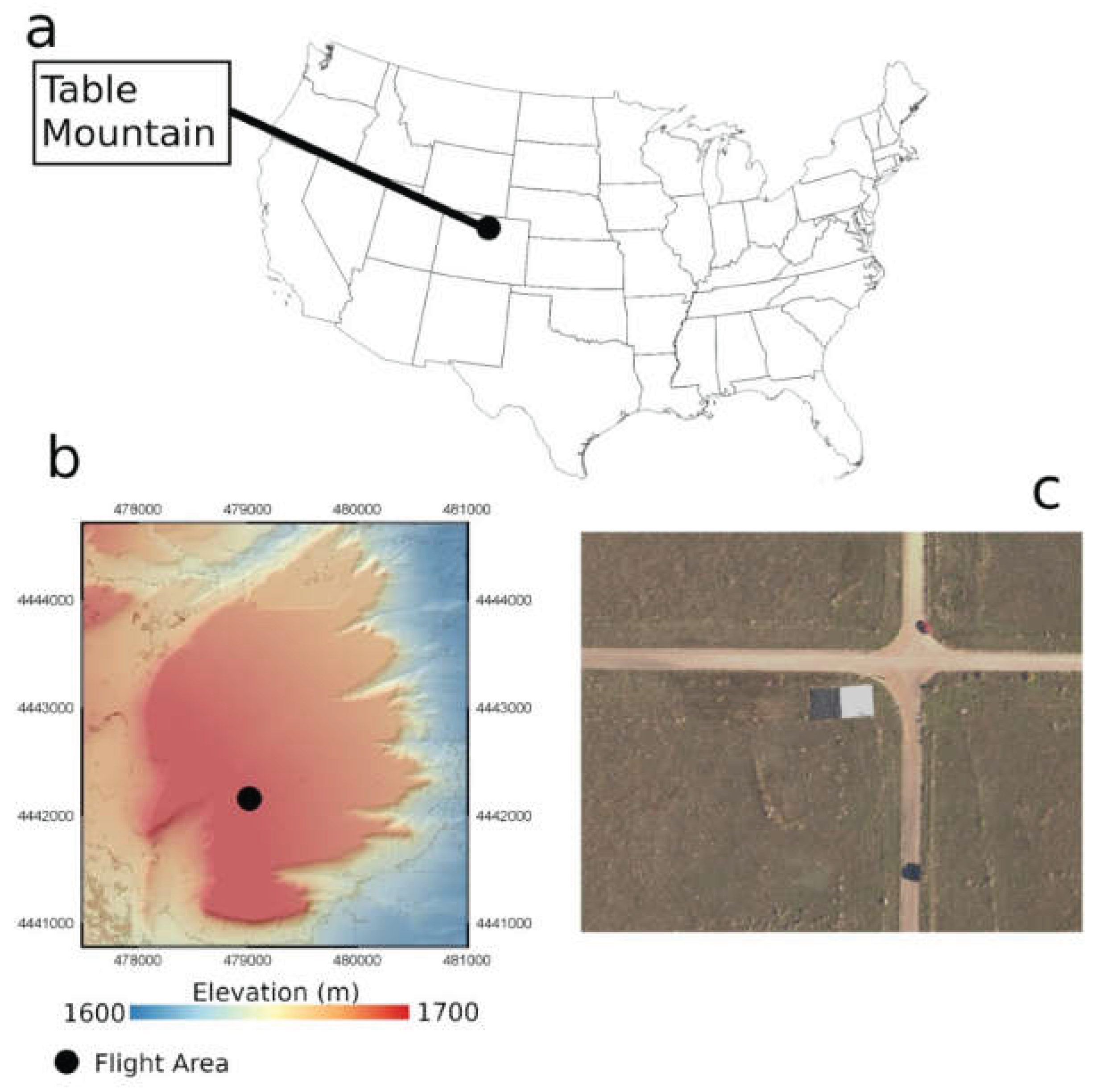
Figure 2.
a) front view of the M210 with the MicaSense RedEdge M [1] and the SlantRange 3p [2], attached to the right and left downward facing gimbals, respectively; b) birds-eye view of the M210 showing the MicaSense DLS and GPS [3] and the SlantRange‘s DLS/GPS component [4]. .
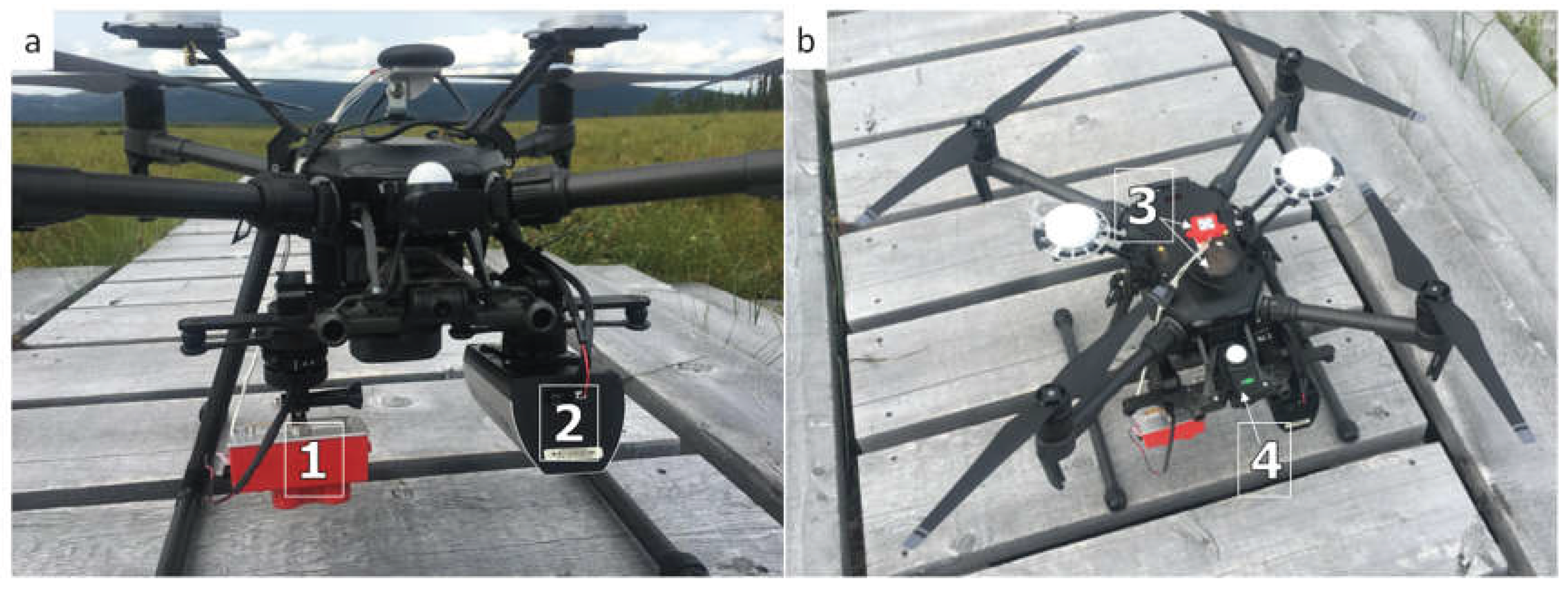
Figure 3.
a) Screenshot of the Drone Deploy software showing the UAV flight area with east-west flight pattern (the tarps are slightly visible here); b) Looking south-southwest over the flight area. Sunny conditions and good visibility persisted during the flight campaign; c) birds-eye view of the northeast quadrant of the flight area. Photo was taken by a DJI Phantom 4 (DJI Inc, DJI Inc., Shenzhen, China) prior to the flight campaign.
Figure 3.
a) Screenshot of the Drone Deploy software showing the UAV flight area with east-west flight pattern (the tarps are slightly visible here); b) Looking south-southwest over the flight area. Sunny conditions and good visibility persisted during the flight campaign; c) birds-eye view of the northeast quadrant of the flight area. Photo was taken by a DJI Phantom 4 (DJI Inc, DJI Inc., Shenzhen, China) prior to the flight campaign.
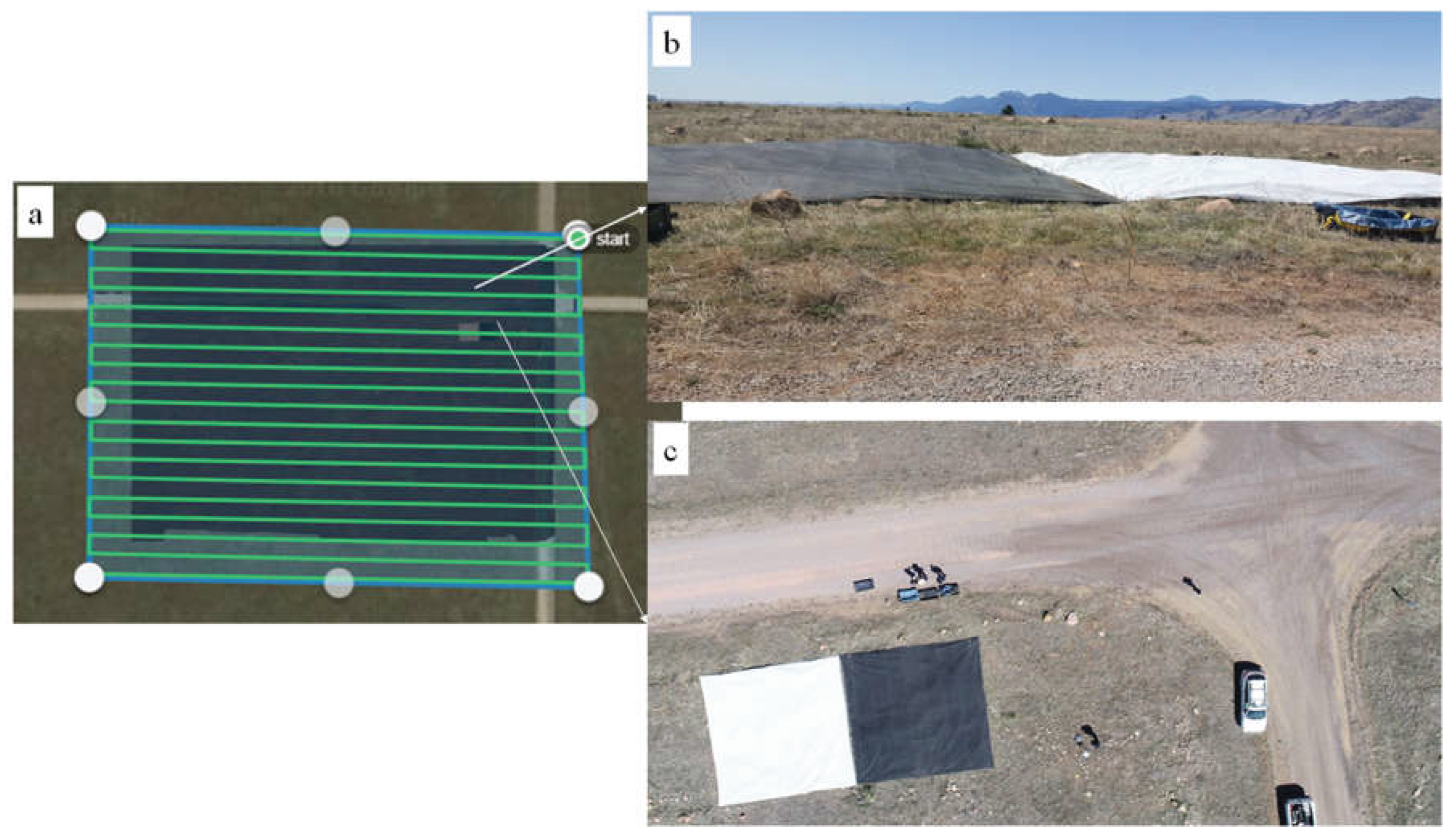
Figure 4.
Reflectance differences between MicaSense and MicaSense resampled NIS values for the 5 Micasesne measurement bands (a - band 1[blue]; b - band 2[green]; c - band 3[red]; d - band 4[LIR]; e - band 5[NIR]) and (f) difference in calculated NDVI from each instrument.
Figure 4.
Reflectance differences between MicaSense and MicaSense resampled NIS values for the 5 Micasesne measurement bands (a - band 1[blue]; b - band 2[green]; c - band 3[red]; d - band 4[LIR]; e - band 5[NIR]) and (f) difference in calculated NDVI from each instrument.
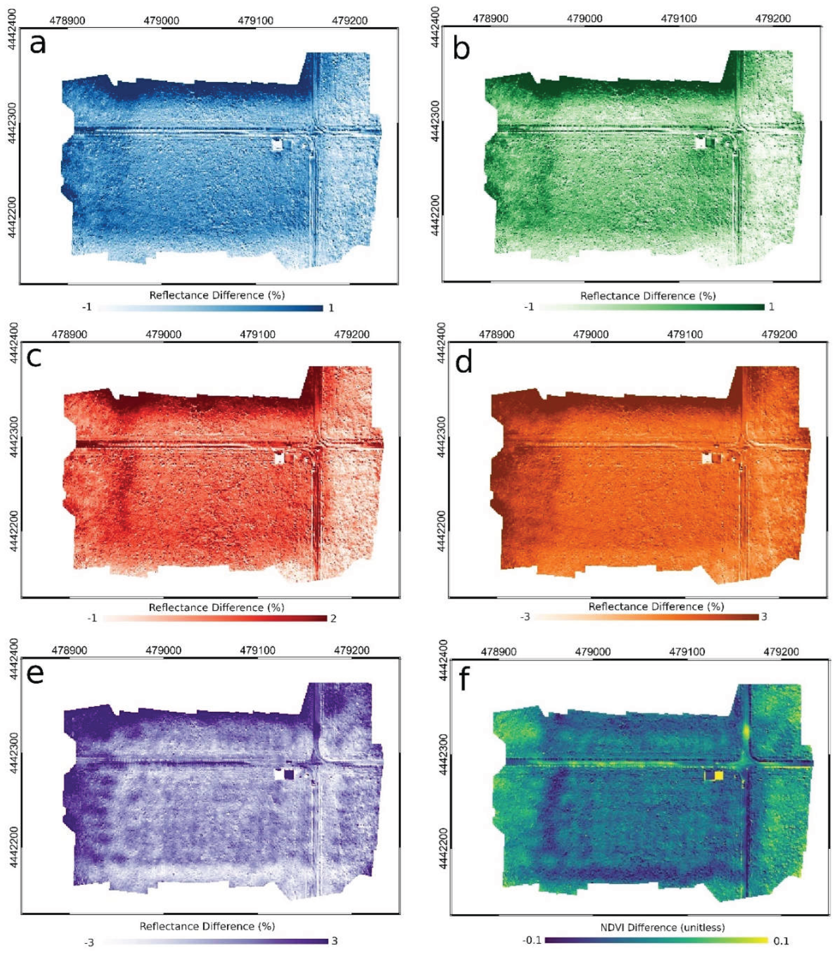
Figure 5.
Scatterplot of reflectance values from the MicaSense and the MicaSense resampled NIS values for the 5 MicaSense measurement bands: a) - band 1[blue]; b) - band 2[green]; c) - band 3[red]; d) - band 4[LIR]; e) - band 5[NIR].
Figure 5.
Scatterplot of reflectance values from the MicaSense and the MicaSense resampled NIS values for the 5 MicaSense measurement bands: a) - band 1[blue]; b) - band 2[green]; c) - band 3[red]; d) - band 4[LIR]; e) - band 5[NIR].
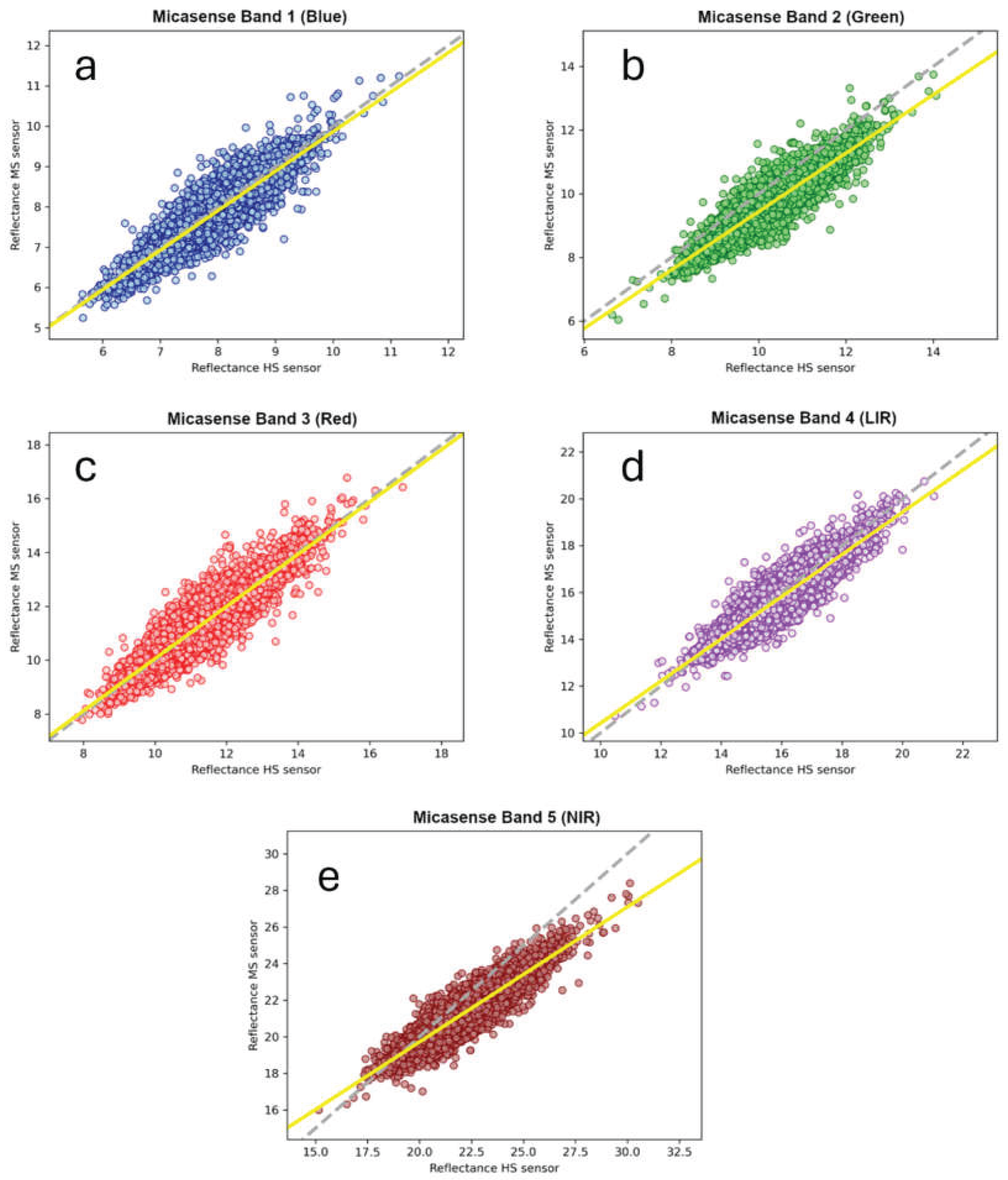
Figure 6.
Reflectance differences between SlantRange and SlantRange resampled NIS values for the 4 SlantRange measurement bands: a) - band 1[green]; b) - band 2[red]; c) - band 3[LIR]; d) - band 4[NIR]); and e) difference in calculated NDVI from each instrument.
Figure 6.
Reflectance differences between SlantRange and SlantRange resampled NIS values for the 4 SlantRange measurement bands: a) - band 1[green]; b) - band 2[red]; c) - band 3[LIR]; d) - band 4[NIR]); and e) difference in calculated NDVI from each instrument.
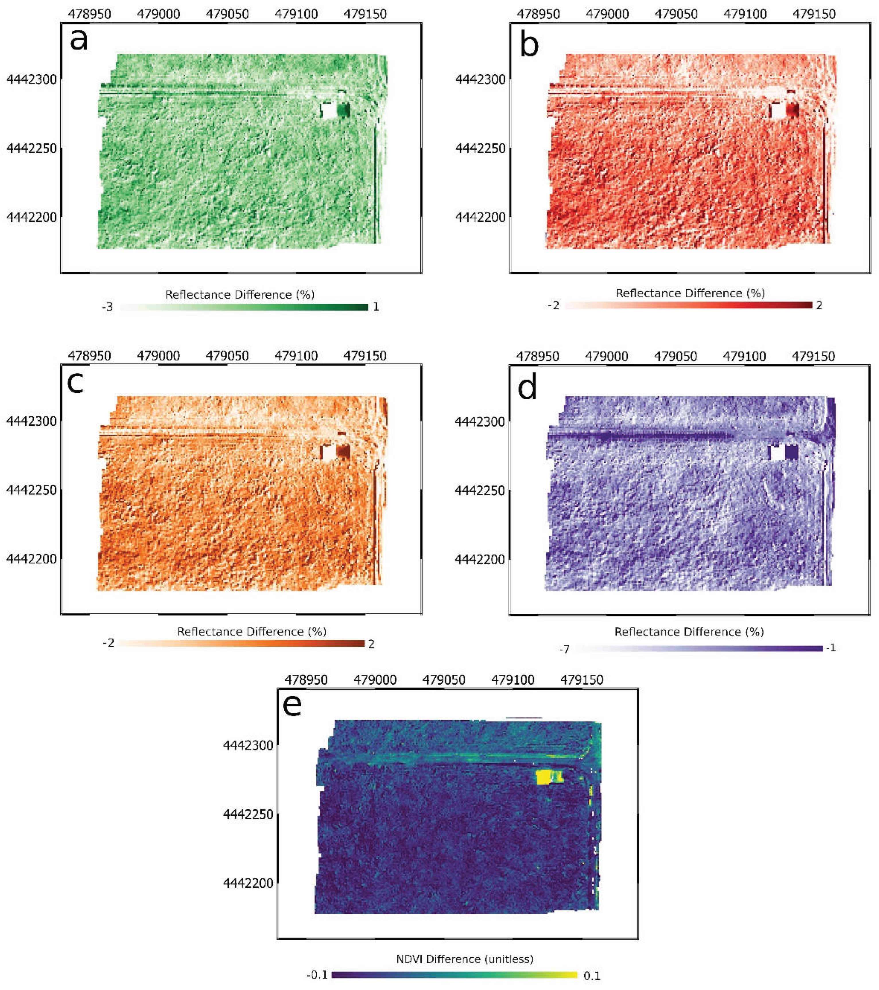
Figure 7.
Scatterplot of reflectance values from the SlantRange and the SlantRange resampled NIS values for the 4 SlantRange measurement bands: a) - band 1[green]; b) - band 2[red]; c) - band 3[LIR]; d) - band 4[NIR].
Figure 7.
Scatterplot of reflectance values from the SlantRange and the SlantRange resampled NIS values for the 4 SlantRange measurement bands: a) - band 1[green]; b) - band 2[red]; c) - band 3[LIR]; d) - band 4[NIR].
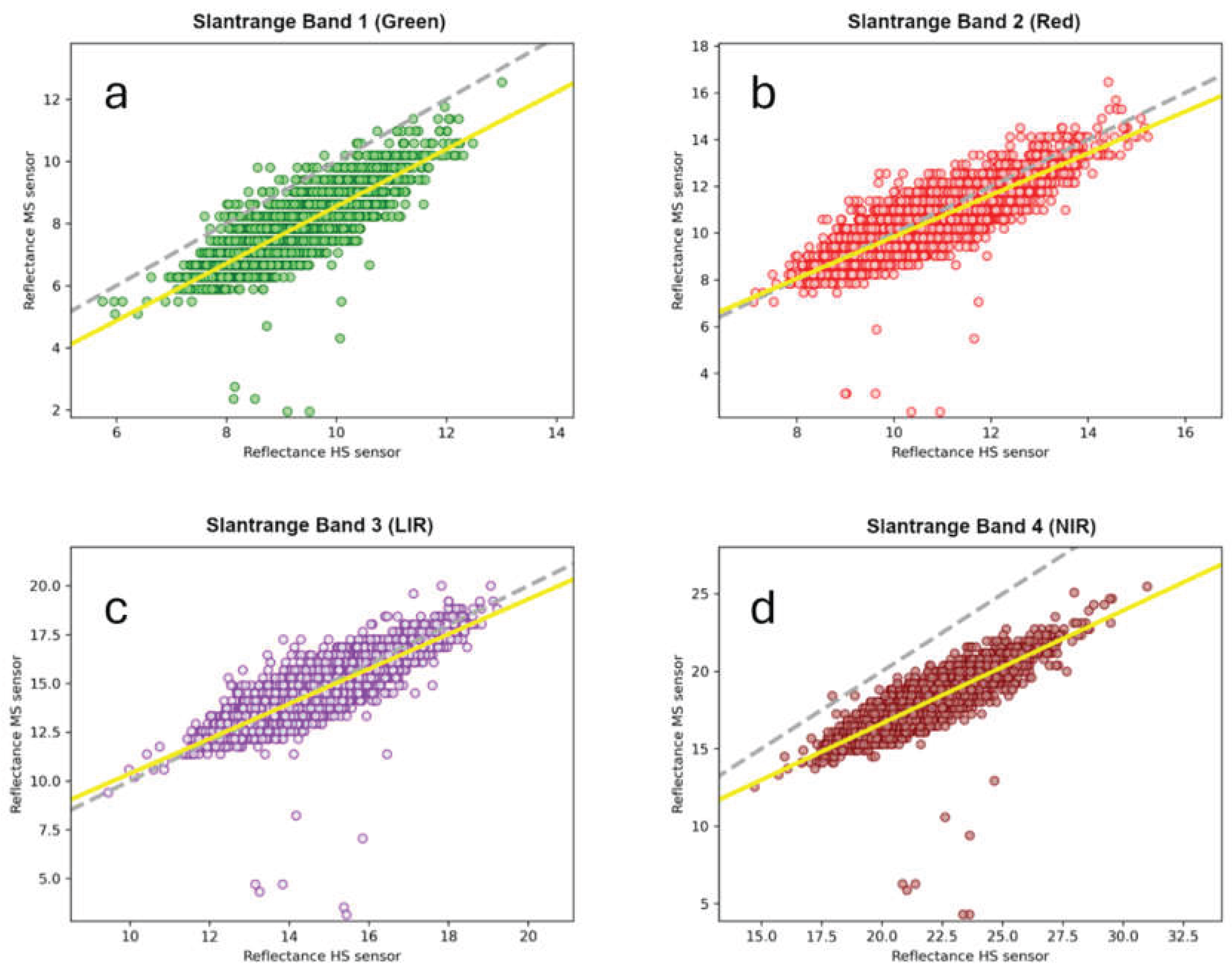
Figure 8.
Differences in calculated NDVI between the NIS and the UAS multispectral sensors, MicaSense and SlantRange.
Figure 8.
Differences in calculated NDVI between the NIS and the UAS multispectral sensors, MicaSense and SlantRange.
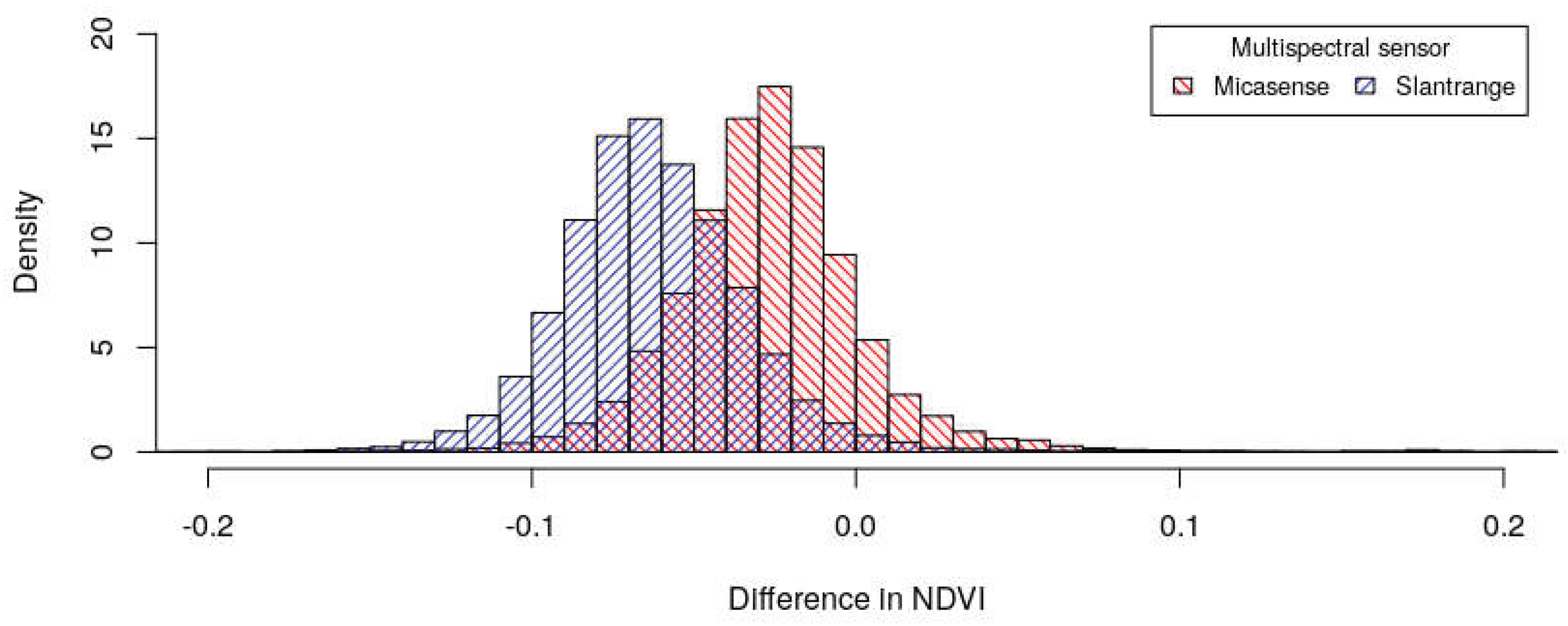
Figure 9.
a)Histogram of reflectance values for different visible wavelength bands over live vegetation. b) Reflectance values over measured wavelengths for live and senescent vegetation.
Figure 9.
a)Histogram of reflectance values for different visible wavelength bands over live vegetation. b) Reflectance values over measured wavelengths for live and senescent vegetation.
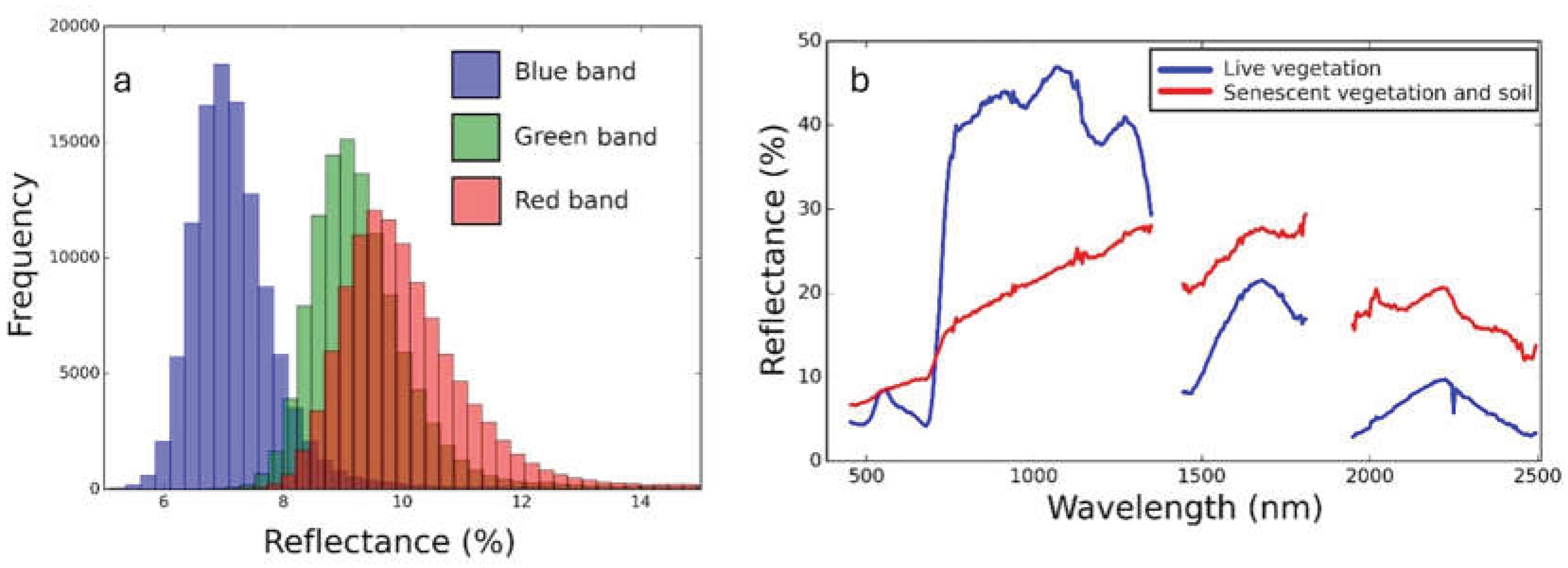

Table 1.
Multispectral sensor specification information.
| MicaSense RedEdge-Ma |
SlantRange 3pb |
|
|---|---|---|
 |
 |
|
|
Spectral Bandsc (nm) Blue Green Red LIR (Leading Infrared) Near-infrared (NIR) |
475 ± 20 560 ± 20 668 ± 10 717 ± 10 840 ± 40 |
NA 550 ± 40 650 ± 40 710 ± 20 850 ± 20 |
| Focal Length (mm) | 5.4 | 12 |
| Focal Plane (mm) | 4.8 x 3.6 | 5.76 x 4.53 |
| Resolution (pixel) | 1280 x 960 | 1280 x 1024 |
| GSD at 120m AGL2d (cm) | 8.2 | 4.8 |
| Output Formats | .TIFF | .DNG | .KML | .SHP | .GeoTIFF |
| Dimensions (mm) | 94 x 63 x 46 | 146 x 69 x 57 |
| Weight (g) | 170 | 350 |
Table 2.
Table of reflectance values for the ASD, MicaSense sensor, and the MicaSense resampled NIS sampling lines (1-3) over the reflectance calibration targets (high – Tarp 48; low - Tarp 03), vegetation, and the road.
Table 2.
Table of reflectance values for the ASD, MicaSense sensor, and the MicaSense resampled NIS sampling lines (1-3) over the reflectance calibration targets (high – Tarp 48; low - Tarp 03), vegetation, and the road.
| ASD | MicaSense | NIS Line 1 | NIS Line 2 | NIS Line 3 | |
| Band 1 | |||||
| Tarp 48 | 49.41 | 50.21±1.04 | 51.83±0.94 | 52.56±0.99 | 51.70±1.16 |
| Tarp 03 | 2.37 | 3.87±0.21 | 3.35±0.18 | 3.40±0.16 | 3.66±0.14 |
| Veg | N/A | 7.36±0.51 | 7.44±0.47 | 7.42±0.46 | 6.98±0.43 |
| Road | N/A | 11.86±0.54 | 11.87±0.50* | 11.97±0.55* | 11.99±2.42* |
| Band 2 | |||||
| Tarp 48 | 49.97 | 47.62±0.96 | 50.60±0.93 | 51.37±1.01 | 50.64±1.14 |
| Tarp 03 | 2.47 | 4.07±0.33 | 3.23±0.15 | 3.31±0.14 | 3.54±0.17 |
| Veg | N/A | 9.06±0.53 | 9.51±0.49 | 9.49±0.48 | 8.94±0.45 |
| Road | N/A | 14.51±0.54 | 14.47±0.53* | 14.64±0.59 | 14.45±2.55* |
| Band 3 | |||||
| Tarp 48 | 50.05 | 48.15±0.98 | 50.78±0.94 | 51.53±1.03 | 50.88±1.17 |
| Tarp 03 | 2.55 | 4.23±0.32 | 3.23±0.16 | 3.30±0.15 | 3.52±0.18 |
| Veg | N/A | 10.34±0.71 | 10.14±0.64 | 10.11±0.63 | 9.55±0.58 |
| Road | N/A | 17.59±0.85 | 16.64±0.79 | 16.77±0.82 | 16.39±2.86 |
| Band 4 | |||||
| Tarp 48 | 50.12 | 47.03±1.03 | 49.91±0.94 | 50.66±1.02 | 50.06±1.13 |
| Tarp 03 | 2.62 | 5.00±0.43 | 3.24±0.17 | 3.32±0.16 | 3.55±0.19 |
| Veg | N/A | 14.88±0.68 | 14.59±0.66 | 14.52±0.63 | 13.71±0.64 |
| Road | N/A | 18.55±0.75 | 17.67±0.67 | 17.85±0.67 | 17.32±3.01 |
| Band 5 | |||||
| Tarp 48 | 50.54 | 43.36±0.85 | 50.93±0.98 | 51.51±1.07 | 51.01±1.16 |
| Tarp 03 | 2.73 | 7.57±0.40 | 3.34±0.20 | 3.39±0.19 | 3.55±0.21 |
| Veg | N/A | 20.65±0.96 | 21.63±1.17 | 21.43±1.12 | 20.34±1.17 |
| Road | N/A | 20.65±0.62 | 19.92±0.61* | 20.00±0.60* | 19.19±3.30 |
*Does not show significant difference.
Table 3.
Table of reflectance values for the ASD, SlantRange sensor, and the SlantRange resampled NIS sampling lines (1-3) over the reflectance calibration targets (high – Tarp 48; low - Tarp 03), vegetation, and the road.
Table 3.
Table of reflectance values for the ASD, SlantRange sensor, and the SlantRange resampled NIS sampling lines (1-3) over the reflectance calibration targets (high – Tarp 48; low - Tarp 03), vegetation, and the road.
| ASD | SlantRange | NIS Line 1 | NIS Line 2 | NIS Line 3 | |
| Band 2 | |||||
| Tarp 48 | 50.01 | 23.27±0.54 | 51.00±0.94 | 51.60±1.02 | 50.89±1.15 |
| Tarp 03 | 2.47 | 3.26±0.34 | 3.19±0.15* | 3.23±0.14* | 3.45±0.17 |
| Veg | N/A | 7.48±0.54 | 9.18±0.51 | 9.11±0.50 | 8.57±0.46 |
| Road | N/A | 11.88±0.86 | 14.34±0.53 | 14.37±0.59 | 14.22±2.54 |
| Band 3 | |||||
| Tarp 48 | 50.30 | 29.41±0.53 | 50.74±0.94 | 51.34±1.05 | 50.75±1.17 |
| Tarp 03 | 2.58 | 4.31±0.52 | 3.18±0.17 | 3.22±0.16 | 3.41±0.19 |
| Veg | N/A | 9.77±0.70 | 10.29±0.68 | 10.21±0.67 | 9.64±0.62 |
| Road | N/A | 14.79±1.12 | 17.36±0.85 | 17.37±0.87 | 16.95±2.96 |
| Band 4 | |||||
| Tarp 48 | 50.37 | 39.14±0.63 | 50.32±0.96 | 50.88±1.06 | 50.33±1.16 |
| Tarp 03 | 2.63 | 4.93±0.61 | 3.16±0.18 | 3.19±0.18 | 3.41±0.20 |
| Veg | N/A | 13.62±0.74 | 14.35±0.66 | 14.22±0.64 | 13.43±0.64 |
| Road | N/A | 16.47±0.81 | 18.23±0.72 | 18.26±0.73 | 17.72±3.13 |
| Band 5 | |||||
| Tarp 48 | 50.58 | 42.67±0.94 | 51.05±0.98 | 51.60±1.08 | 51.11±1.16 |
| Tarp 03 | 2.63 | 5.07±0.86 | 3.37±0.19 | 3.41±0.19 | 3.57±0.21 |
| Veg | N/A | 17.45±1.00 | 22.15±1.18 | 21.94±1.13 | 20.85±1.19 |
| Road | N/A | 16.37±0.60 | 20.04±0.60 | 20.11±0.59 | 19.33±3.33 |
*Does not show significant difference.
Disclaimer/Publisher’s Note: The statements, opinions and data contained in all publications are solely those of the individual author(s) and contributor(s) and not of MDPI and/or the editor(s). MDPI and/or the editor(s) disclaim responsibility for any injury to people or property resulting from any ideas, methods, instructions or products referred to in the content. |
© 2026 by the authors. Licensee MDPI, Basel, Switzerland. This article is an open access article distributed under the terms and conditions of the Creative Commons Attribution (CC BY) license (http://creativecommons.org/licenses/by/4.0/).
Copyright: This open access article is published under a Creative Commons CC BY 4.0 license, which permit the free download, distribution, and reuse, provided that the author and preprint are cited in any reuse.


