

Submitted:
29 June 2026
Posted:
30 June 2026
You are already at the latest version
Abstract
Flood events in agricultural floodplains reflect not only the intensity of rainfall but the vulnerability of the land surface at the moment of the event. This study examines the January–February 2026 flood in Larache Province, Morocco, through an integrated remote sensing workflow combining Sentinel-1 SAR imagery, CHIRPS precipitation data, and Dynamic World land cover within Google Earth Engine, processed via the rgee R package. Flood extent was mapped using SAR backscatter change detection and validated against rainfall dynamics. Land cover conditions were assessed across four temporal windows — spring 2025, pre-event, post-event, and spring 2026 — to evaluate how the landscape entered the event and how it recovered. Results show that a significant share of normally cultivated land was in a bare soil state before the flood, increasing runoff generation and susceptibility to inundation. Post-flood analysis across 25 sample areas documents spatially uneven recovery, with cropland coverage still below seasonal norms in spring 2026. These patterns reflect structural land use conditions — wetland loss, intensive seasonal agriculture, drought-degraded soils — that amplified the impact of an already severe event. The findings have direct implications for land use management: cover cropping practices, updated flood hazard zoning, and targeted wetland restoration could meaningfully reduce vulnerability in the Loukkos floodplain and in comparable alluvial agricultural systems across the region.
Keywords:
sentinel-1 SAR
; flood mapping
; land cover vulnerability
; agricultural land use
; Loukkos floodplain
; Larache Province
; flood risk management
; Google earth engine
1. Introduction
Flooding is among the most damaging natural hazards affecting agricultural regions worldwide, causing substantial economic losses, threatening food security, and contributing to long-term soil degradation (Kassaw & Nebere, 2025; Rahman & Di, 2020). In Morocco, recurrent flood events have increasingly affected northern and northwestern territories, where heavy rainfall rapidly translates into the inundation of farmland and settlements, generating significant environmental, social, infrastructural, and agricultural impacts (Loudyi et al., 2022). Riverine and flash floods also generate major damage to crops, infrastructure, and livelihoods (Kassaw & Nebere, 2025). Northern and Western Morocco is particularly vulnerable, as shown by documented flood events in Tetouan (Lahsaini et al., 2019), the Gharb Plain, and the Loukkos River basin. The Loukkos basin is especially exposed because the river flows across a gently sloping alluvial plain that favors the lateral expansion and persistence of floodwaters.
The winter of 2025-2026 in Morocco produced severe hydrometeorological disturbances with major environmental, agricultural, and socio-economic consequences. Prolonged and intense rainfall, associated with a succession of deep cold depressions, generated widespread flooding across several low-lying plains and downstream river sectors, particularly in Gharb and Loukkos. As precipitation persisted over several weeks, soils progressively lost their infiltration capacity, promoting generalized surface runoff and the expansion of water over large areas. Seasonal wetlands such as ponds and marshy wetlands filled rapidly, while river discharge increased markedly and dam reservoirs reached critical storage levels.
The agricultural sector was among the most affected. Extensive tracts of farmland were inundated, causing major losses in cereals, sugar beet, vegetable crops, and soft fruit production. Beyond agriculture, the impacts extended to infrastructure and daily life: roads and bridges were damaged, mobility was interrupted, and access to basic services became difficult in several localities. In some cases, settlements were temporarily isolated by floodwaters, with interruptions in electricity, drinking water supply, and road connectivity, which led to evacuations and population displacement.
Accurate and timely mapping of flood extent, duration, and recession is essential to quantify impacts on crops and to support disaster risk management, policy decisions and farmer preparedness (Ghosh et al., 2024). Remote sensing and GIS technologies have proven effective for monitoring floods and assessing agricultural damage (Tavus et al., 2022).
Sentinel-1 SAR satellite data provides high temporal resolution for flood extent mapping (Haghighi, 2022). The use of Sentinel-1 (S1) radar for flood detection offers several critical advantages over traditional optical satellites and older radar missions, primarily due to its technical specifications and systematic acquisition policy (Torres et al., 2012). It has global coverage, as it consists of a constellation of two satellites that can monitor the entire Earth every 6 days, acquiring data systematically with a stable incidence. As a Synthetic Aperture Radar (SAR) mission, Sentinel-1 can monitor land in almost all-weather conditions, including through dense cloud cover and rain and during the night (Torres et al., 2012). This capability is a major advantage for flood mapping, as flooding is often caused by extreme weather events where clouds would hide or obscure the view of optical satellites (Schumann & Moller, 2015).
Sentinel-1 also strongly supports big data and time-series analysis through its systematic and frequent acquisitions, which generate extensive image archives over time. These long time series allow researchers to characterize normal backscatter conditions for each pixel under non-flooded conditions and identify anomalies caused by floods (Pulvirenti et al., 2011; Twele et al., 2016; Gorelick et al., 2017). Access to multiple reference images also helps distinguish permanent low-backscatter surfaces, such as roads or airport runways, from floodwater (Twele et al., 2016). In addition, Sentinel-1 data is openly and freely accessible through the European Space Agency (ESA), while its large data volume can be efficiently processed using cloud computing platforms such as Google Earth Engine (GEE) (Gorelick et al., 2017; Zhu et al., 2011). This cloud-based processing enables rapid management and analysis of large datasets, producing near-real-time results compared with older and more time-consuming manual methods (Zhu et al., 2011).
In Sentinel-1 SAR imagery, VH polarization is particularly sensitive to volume scattering. Although VH is generally more affected by noise (Lee & Pottier, 2017), flood detection can still be effectively implemented using anomaly-based approaches applied to VH polarization time series, where deviations from baseline backscatter conditions indicate potential inundation. To distinguish flooded from non-flooded areas, several automated thresholding techniques have been developed, among which Otsu’s method (Otsu, 1979) is one of the most widely used. Otsu’s method is an automatic image-thresholding algorithm that has demonstrated strong performance in SAR-based flood detection, particularly when combined with multi-temporal change detection approaches (Clement et al., 2018; Pulvirenti et al., 2011). Its effectiveness, combined with dense Sentinel-1 time-series data, makes it well suited for fully automated flood mapping in large-scale and complex environments (Martinis et al., 2015; Schumann & Moller, 2015; Twele et al., 2016).
The present study focuses on the February 2026 floods in Larache province, northern Morocco, aiming to quantify and map flood extent, duration, and recession using multi-temporal Sentinel-1 SAR data using an unsupervised thresholding approach based on Otsu’s method applied to VH backscatter changes, which automatically separates flooded and non-flooded pixels by minimizing intra-class variance. The results demonstrate the effectiveness of SAR-based monitoring for rapid, weather-independent flood assessment and provide critical guidance for farmers and planners in flood-prone regions.
2. Materials and Methods
2.1. Study Area
The study is conducted in the province of Larache, located in the north of Morocco, along the Atlantic coast, within the Tangier-Tetouan-Al Hoceima region. The province comprises 19 communes in total, including 2 urban communes (municipalities) and 17 rural communes.
Figure 1.
(a), (b) Geographical Location of Larache Province within the Moroccan Territory.
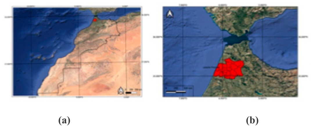
The area is renowned for its river network, variable topography, and intensive agricultural activities, which contribute significantly to national production. The province covers an area of approximately 2,000 km² and lies between 34°30′00′′ to 35°10′00′′ N latitudes and 5°45′00′′ to 6°30′00′′ W longitudes. The province has an altitude range from sea level up to 1654 m.a.s.l. (Figure 2), with slopes varying from 0 to 54° (Figure 3).
The climate is Mediterranean with strong Atlantic influences, characterized by mild, wet winters and warm, dry summers. Geologically, Larache Province is mainly composed of Cretaceous and Tertiary deposits, with alluvial plains along the Oued Loukkos. The most recent significant flooding events in the province occurred in October 2019 and November 2021 and February 2026.
The Loukkos basin is structured around a major hydraulic installation, the Oued El Makhazine Dam, one of Morocco’s most important dams (Bouaicha & Benabdelfadel, 2010). Built on the Loukkos River, the dam stores upstream flows within a reservoir and regulates downstream discharge, serving primarily irrigation and water supply functions. Downstream from the dam, the Loukkos flows toward the Atlantic through a broad marshy depression, a geomorphological setting that contributes to the hydrological sensitivity of the lower valley. Within this fluvial system, Ksar El Kbir is located upstream of Larache within the low-lying alluvial plain of the middle-lower Loukkos valley, whereas Larache occupies a relatively elevated position on the cliffed left bank of the river mouth.
Before the commissioning of the Oued El Makhazine Dam in 1979, followed by a secondary protective dam in 1981, flooding constituted a recurrent feature of the lower Loukkos system. Archaeological and historical evidence suggests that human settlements in the basin have long been shaped by hydraulic risks. Roman settlements and communication routes were strategically established on elevated ridges in order to avoid low-lying flood-prone areas. The ancient site of Lixus, for instance, was built on a rocky hill approximately 80 m above sea level, allowing it to remain protected from seasonal inundation (Ait Oumghar, 2019). During major flood events, the surrounding plain reportedly became so submerged that the hill appeared as an island when viewed from the sea.
In contrast, the settlement of Novum Oppidum, located within the alluvial plain, appears to have been more directly exposed to fluvial dynamics. Its disappearance is thought to be linked to two main factors: the renewal and expansion of Ksar El Kbir during the Almohad era, which led to the destruction and removal of the remaining structures of the ancient city, and the progressive accumulation of alluvial deposits from the Loukkos River between the 12th and 19th centuries, which gradually buried the settlement beneath successive sediment layers (Ait Oumghar, 2019). Nevertheless, the definitive interpretation of the site’s disappearance remains uncertain and would require further archaeological excavations to be fully confirmed (Ait Oumghar, 2019).
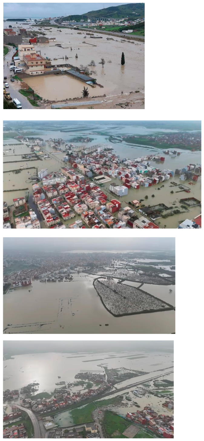
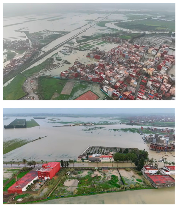
More recent archival evidence indicates that the estuarine zone was frequently inundated and that Ksar El Kbir experienced twelve flood episodes between 1936 and 1951 (Cabanás, 1951). Far from representing an isolated or recent phenomenon, flooding is therefore closely linked to the geomorphological and hydrological functioning of the Loukkos valley. Although the construction of the Oued El Makhazine Dam significantly contributed to reducing flood hazards and regulating water resources within the basin, flood risk was not entirely eliminated. Recent susceptibility assessments continue to identify the Ksar El Kbir–Larache floodplain among the most vulnerable sectors of the basin (Benchbani et al., 2022; Mekkaoui et al., 2026). In this perspective, the February 2026 flood crisis, which triggered large-scale evacuations in Ksar El Kbir, appears less as an isolated disaster than as part of a long historical continuum of recurrent flooding, territorial adaptation, and persistent vulnerability within the lower Loukkos valley.
Figure 4.
Photographs of the 2026 Flood Events in Ksar El Kbir (source : Article19.ma).
2.2. Data Sources
This study adopts an integrated multi-sensor workflow combining multi-temporal precipitation data, Synthetic Aperture Radar (SAR) observations, and satellite-derived land cover information. The analysis is based on the joint use of rainfall data from the Climate Hazards Group InfraRed Precipitation with Stations (CHIRPS) dataset, C-band SAR data acquired by the European Space Agency Sentinel-1 mission, and land cover products from Dynamic World. All datasets were accessed and processed within the Google Earth Engine environment through the rgee package in R (Aybar et al., 2020).
The Climate Hazards Group InfraRed Precipitation with Stations (CHIRPS) dataset integrates satellite-based infrared observations with in-situ rain gauge measurements to provide quasi-global precipitation estimates, particularly suited for regions with limited ground-based monitoring (Funk et al., 2015). CHIRPS is characterized by a spatial resolution of approximately 0.05° (~5 km) and a temporal resolution of one day, offering a reliable representation of rainfall dynamics at a regional scale. The variable considered in this study is daily precipitation, expressed in millimeters per day and defined as P(x,t)[mm/day], where x denotes the spatial location and t the temporal dimension. The analysis focuses on the Area of Interest (AOI) Larache-Ksar El Kebir and covers the period between January and February 2026, corresponding to the pre-event and event/post-event phases of the observed flood.
The Sentinel-1 mission provides C-band SAR data acquired in Interferometric Wide Swath (IW) mode, with a spatial resolution of approximately 10 m and a revisit time of 6-12 days depending on orbital configuration (Torres et al., 2012). SAR data are particularly suitable for flood detection due to their sensitivity to surface roughness and dielectric properties, as well as their capability to operate independently of cloud cover and illumination conditions (Schumann & Moller, 2015). In this study, Ground Range Detected (GRD) products with dual polarization (VV and VH) were used, with a specific focus on the VH channel, which has been shown to be more responsive to surface water-induced backscatter reductions (Twele et al., 2016).
To support the interpretation of flood dynamics in relation to land surface characteristics, land cover information was derived from the Dynamic World dataset. Dynamic World provides near real-time global land cover classification at 10 m spatial resolution, generated from Sentinel-2 imagery using a deep learning framework (Brown et al., 2022). The dataset includes nine land cover classes (water, trees, grass, flooded vegetation, crops, shrub and scrub, built area, bare ground, and snow/ice). In this study, categorical land cover maps were derived using the modal class over defined temporal windows representing pre-event baseline conditions (October-November 2025), event/post-event conditions (January-February 2026), and a pre-event spring growing season (March-May 2025), used to characterize seasonal land cover dynamics under non-flooded conditions. The near-real time temporal segmentation enables a consistent comparison between baseline land cover conditions, immediate flood impacts, and pre-event dynamics.
2.3. Methods
This study adopts a sequential, data-driven workflow integrating satellite-derived precipitation data, SAR observations, and land cover information to characterize flood dynamics and their interaction with surface conditions. Precipitation patterns are first analyzed to identify critical temporal windows associated with hydrological response, which are subsequently used to guide SAR-based flood detection. Daily precipitation data from the CHIRPS dataset were analyzed over the period 1 January-28 February 2026, capturing both pre-conditioning and peak rainfall phases in the Larache region. To characterize rainfall accumulation, the study period was subdivided into four consecutive 15-day intervals. For each interval t, cumulative precipitation was computed (as shown in Formula 1):
where represents daily rainfall (mm) and n=15 days. This metric captures the temporal integration of precipitation and serves as a proxy for hydrological loading, commonly used to interpret runoff generation processes (Oberstadler et al., 1998). For each interval, spatial statistics including minimum, maximum, mean, and 95th percentile were derived over the Area of Interest (AOI), with the latter used to characterize high-intensity rainfall while limiting sensitivity to outliers. A daily rainfall time series was also computed by spatially averaging precipitation over the AOI, enabling the identification of rainfall peaks and cumulative hydrological loading preceding flood occurrence.
Flood extent was derived from Sentinel-1 C-band SAR data using a multi-temporal anomaly-based approach. GRD images acquired in Interferometric Wide Swath (IW) mode and VH polarization were selected over a pre-event reference period (15-24 January 2026) and an event window (25 January-10 February 2026), defined based on rainfall dynamics. SAR-based flood detection relies on the strong contrast between open water and surrounding surfaces, where smooth water bodies induce a marked decrease in backscatter due to specular reflection (Oberstadler et al., 1998; Amitrano et al., 2021). VH polarization has been shown to enhance the detection of inundated areas and improve class separability, particularly in heterogeneous and vegetated environments (Carreño Conde and De Mata Muñoz, 2019).
Multi-temporal SAR analysis enables the detection of flood-induced changes by comparing event conditions against pre-event baseline states and has been widely applied for rapid flood mapping in complex environments (Tay et al., 2020) and in operational early warning frameworks (Sujono et al., 2026). For each period, SAR image collections were aggregated using the median to reduce scene-specific variability, and a focal median filter (60 m radius) was applied to mitigate speckle noise while preserving spatial structures.
A pre-event baseline was constructed by computing the mean and standard deviation of the VH backscatter signal (as shown in Formula 2, 3):
where N is the number of pre-event observations. The event backscatter was compared to baseline conditions to derive the anomaly (Formula 4):
and standardized using a z-score (Formula 5):
An adaptive threshold was applied to the anomaly distribution using Otsu’s method (Otsu, 1979), enabling data-driven separation between flooded and non-flooded pixels. Histogram-based thresholding approaches are adopted in SAR flood mapping due to their robustness and effectiveness (Carreño Conde and De Mata Muñoz, 2019; Amitrano et al., 2021). To ensure conservative detection, the threshold was constrained to negative values and combined with a z-score condition to isolate strong backscatter reductions associated with inundation. Flooded pixels were defined as (Formula 6):
The resulting flood mask was refined through light spatial filtering. A morphological filter was applied to reduce isolated noise, followed by connected pixel analysis retaining only clusters with at least five connected pixels. A slope-based constraint derived from the SRTM digital elevation model was then applied, retaining only areas with slope values below 6°. The robustness of the VH anomaly threshold was evaluated through a sensitivity analysis by varying histogram construction parameters, including the number of bins (64–128), minimum bucket width (0.05-0.2), and spatial aggregation scale (90-150 m).
Finally, the SAR-derived flood mask was integrated with Dynamic World land cover data. Land cover maps were generated using the modal class over three temporal windows: pre-event baseline (October-November 2025), event/post-event conditions (January-February 2026), pre-event and post-event spring growing season (March-May 2025, and March-May 2026). The use of temporally aggregated land cover products reduces classification noise and improves the stability of land surface representation under dynamic environmental conditions (Tay et al., 2020). The flood mask was applied to each land cover layer (Formula 7):
allowing the computation of class-wise flooded area and percentage and enabling a comparative assessment of flood exposure across land cover types and temporal conditions.
A site-level analysis was conducted across 25 sample areas spatially distributed throughout the SAR-derived flood footprint. Sample areas were delineated as square polygons of approximately 15 km² and selected to provide coverage of the full range of flood intensities, land cover types, and positions relative to the Loukkos River corridor documented within the study domain. For each area, Dynamic World land cover maps were extracted for the same four temporal windows used in the area-wide analysis: pre-event baseline (Oct–Nov 2025), event/post-event (Jan–Feb 2026), spring growing season 2025 (Mar–May 2025), and spring growing season 2026 (Mar–May 2026). Each area is visualised as a five-panel composite displaying the SAR-derived flood overlay on the satellite image alongside the four temporal land cover maps, enabling direct visual comparison of land surface conditions before, during, and after the flood event across spatially contrasting settings.
3. Results
The results of the workflow are presented through a multi-scale analysis integrating precipitation patterns, SAR-derived flood extent, and land cover information. Rainfall dynamics are first quantified to identify the temporal windows associated with peak hydrological forcing. These intervals are subsequently used to interpret SAR backscatter anomalies and derive flood extent. Finally, the integration with Dynamic World land cover data enables the quantification of flood exposure across different surface classes, providing insight into the spatial distribution of flood impacts.
3.1. CHIRPS Rainfall Aggregation and 15-Day Interval Statistics
The 15-day rainfall aggregation highlights a clear temporal variability in precipitation across the study period, with a strong concentration of rainfall during late January and early February 2026 (Table 1). Rainfall conditions during the first interval (01-15 January) were moderate, with a mean precipitation of 76.42 mm and limited spatial variability (P95 = 91.64 mm). A substantial increase occurred in the second interval (16-30 January), representing the peak rainfall phase, with mean values reaching 283.50 mm and maximum values exceeding 350 mm. The high P95 (321.71 mm) indicates widespread high-intensity rainfall across the AOI. The third interval (31 January-14 February) maintained elevated precipitation levels, although slightly lower than the peak phase (mean = 255.92 mm; max = 367.28 mm). The persistence of high P95 values (310.23 mm) suggests sustained hydrological pressure. In contrast, the final interval (15-28 February) shows a sharp decrease in precipitation (mean = 5.02 mm; max < 20 mm), marking the end of the rainfall event. The spatial distribution of cumulative rainfall (Figure 5) highlights the emergence of precipitation hotspots during the peak intervals, particularly in the central and eastern sectors of the AOI. The temporal progression clearly delineates the transition from moderate pre-conditioning rainfall to peak event conditions, followed by a rapid decay phase.
CHIRPS daily time series analysis and event-window identification
To identify the rainfall event window relevant for the SAR-based flood analysis, the CHIRPS daily precipitation series was analyzed using a dual-axis graph combining daily and cumulative rainfall. Daily rainfall was represented as bars, while cumulative rainfall was plotted as a continuous curve. Due to their different numerical ranges, the cumulative series was rescaled for visualization, while its original values were preserved on the secondary axis (Figure 6). Based on the observed temporal pattern, the period 25 January to 10 February 2026 was identified as the main event window, capturing the phase of sustained precipitation likely responsible for flood triggering and guiding the Sentinel-1 analysis. The combined interpretation of daily and cumulative rainfall supports the hydrometeorological characterization of the event, distinguishing between short-term rainfall peaks and cumulative surface loading.
3.2. SAR-Based Flood Detection and Backscatter Anomaly Analysis
The SAR analysis picks up from the event window identified in the CHIRPS data, covering 25 January to 10 February 2026, with the period 15–24 January serving as the pre-event baseline. Multi-temporal Sentinel-1 VH backscatter is compared against that baseline to produce anomaly and z-score maps, from which flood-affected pixels are separated. The VH anomaly map (Figure 7) shows the full range of backscatter change across the AOI, spanning −17.29 to 10.03. Most of the territory sits close to zero, displayed as uniform light blue, indicating conditions broadly consistent with the baseline. The darker patches concentrated in the central-western sector trace the areas where backscatter dropped most sharply, following the main drainage network and the low-lying ground alongside it. Applying the Otsu-derived threshold of −2.19 captures 8,603.74 ha (3.15% of the AOI) below this cut-off, identifying the spatially coherent zones of signal reduction most likely linked to inundation.
The VH z-score map (Figure 8) places anomaly values in the context of baseline temporal variability, making it possible to identify deviations that are statistically unusual rather than simply negative. Values range from −216.88 to 69.50. The darkest tones, concentrated along the central-western drainage corridor, correspond to pixels where backscatter dropped well below what the baseline record would predict. Pixels with z-scores below −1.7 cover 12,560.25 ha (4.59% of the AOI), a broader area than the anomaly estimate alone, reflecting the greater sensitivity of the z-score to relative rather than absolute signal change. Applying both thresholds together, then removing isolated clusters and steep terrain, brings the final flood extent to 6,657.57 ha (2.44% of the AOI), as shown in Figure 9. The flooded area follows the main river corridor and adjacent floodplain in the central-western sector, with smaller scattered patches in the south.
The histogram (Figure 10) and a parameter sensitivity test (Figure 11) together confirm that the threshold is well-founded. The VH anomaly distribution is strongly right-skewed: most pixels fall between 0 and 1, with peak frequencies above 40,000, which matches the predominantly stable surface visible in Figure 7. The negative tail thins out quickly below −1.8, dropping from roughly 2,000 pixels there to around 1,300 at −2.19 and below 1,000 for more negative values. The Otsu threshold lands precisely at that inflection point, where the sparse anomalous pixels separate cleanly from the main distribution. The flood class is small relative to the full pixel population, but it is statistically distinct. The sensitivity test (Figure 11) shows the threshold holding at −2.19 across all 20 histogram parameter combinations tested. A few points under the coarsest settings drift toward −2.6 to −2.7, but this does not shift the dominant solution. The near-horizontal reference line and tight clustering of observed values confirm that the threshold is stable across parameter choices.
3.3. Land Cover Flood Impact Assessment
The land cover assessment overlays the SAR flood mask on Dynamic World classifications to quantify how much of each surface class was affected, across four temporal snapshots. Because Dynamic World reflects actual conditions at the time of each acquisition, the class distributions capture what the land was doing at each moment rather than a fixed category label. Under pre-event conditions (Table 2), croplands made up 58.06% of the flooded footprint, with bare soil (15.15%) and shrub and scrub (11.97%) accounting for most of the remainder. The areas that were later inundated were largely in agricultural use or partially exposed before the event. During the flood period (Table 3), water became the dominant class at 56.80%, with bare soil (14.52%) and flooded vegetation (8.95%) following. This shift shows how cropland and other vegetated surfaces were submerged or waterlogged across much of the SAR-detected flood extent. The 2025 spring growing season (Table 4) provides a seasonal benchmark: croplands covered 70.10% of the same footprint at that time, and water accounted for only 6.33%, reinforcing how anomalous the flood-period conditions were. The 2026 spring growing season (Table 5) tells a different story. Croplands had recovered somewhat but remained lower than in 2025 (45.28% versus 70.10%), while bare soil was substantially higher (16.45% versus 3.84%) and water coverage had not fully receded (17.01% versus 6.33%). Grass also expanded compared to 2025 (9.82% versus 8.69%). These differences suggest that the flood left a detectable imprint on the land surface well into the following growing season, with some areas remaining waterlogged or unplanted several months after the event. The full class distributions across all four conditions are shown in Figure 12.
3.4. Site-Level Land Cover Analysis of Flood-Affected Areas
To complement the area-wide flood Land Use Classification mapping presented in Section 3.2, a site-level analysis was carried out across 25 sample areas distributed throughout the SAR-derived flood footprint (Figure 13). For each area, Dynamic World land cover maps were extracted for four temporal windows: spring 2025 (Mar–May 2025), pre-event (Oct–Nov 2025), post-event (Jan–Feb 2026), and spring 2026 (Mar–May 2026). Together, these comparisons provide a spatially disaggregated view of flood impact and recovery across heterogeneous land surface conditions within the affected floodplain (Figure 14, Figure 15, Figure 16, Figure 17, Figure 18, Figure 19, Figure 20, Figure 21, Figure 22, Figure 23, Figure 24, Figure 25, Figure 26, Figure 27, Figure 28, Figure 29, Figure 30, Figure 31, Figure 32, Figure 33, Figure 34, Figure 35, Figure 36, Figure 37 and Figure 38).
The 25 sample areas capture the full spectrum of flood exposure, pre-event land cover conditions, and post-event recovery trajectories across the Larache Province study domain. Along the main Loukkos floodplain corridor, inundation during Jan–Feb 2026 is near-total in several areas: Area 2 (Figure 15) and Area 3 (Figure 16) in the lower valley record combined water and flooded vegetation fractions of 55.9% and 45.0% respectively, while Area 4 (Figure 17) and Area 14 (Figure 27) in the south-central alluvial plain show similarly extensive coverage — the latter particularly striking given its pre-event crop dominance of 95.3%, which collapsed to 19.6% post-event and recovered only partially to 58.8% by spring 2026. Areas 5 (Figure 18), 8 (Figure 21), and 12 (Figure 25) in the central plain show spatially variable inundation controlled by surface drainage patterns and local topography, with flooded vegetation emerging as a dominant post-event class along drainage corridors. Across the floodplain, pre-event bare soil was consistently converted to water or flooded vegetation in the post-event window: most clearly in Area 9 (Figure 22) and Area 19 (Figure 32) — where pre-event bare fractions of 21.7% and 9.5% collapsed to 5.6% and near-zero — but equally pronounced in Area 11 (Figure 24), where 32.9% pre-event bare soil fell to 3.3%, and in Area 25 (Figure 38), where the highest bare fraction in the dataset (48.4%, reflecting exposed reservoir substrate) was almost entirely converted to water (0.4% post-event). This bare-to-water conversion reflects how pre-event soil exposure amplifies inundation extent under equivalent rainfall forcing, through reduced infiltration capacity and greater surface runoff connectivity. The reverse pattern appears in Areas 10 (Figure 23) and 19 (Figure 32), where bare soil fractions increase post-event — from 3.2% to 18.2% and from 9.5% to 19.3% respectively — pointing to localised sediment deposition or vegetation loss during flood recession. A similar post-flood bare soil increase is evident in spring 2026 in Areas 4 (Figure 17) and 5 (Figure 18), where bare fractions rise to 36.1% and 30.7%, well above pre-event levels, possibly reflecting residual sediment deposits or delayed crop failure on waterlogged soils. Area 15 (Figure 28) shows extensive post-event inundation within the river footprint, with flooded vegetation persisting at the wetland margins into the spring period. Along the riparian corridors, Areas 13, 16, and 21 (Figure 26, Figure 29 and Figure 34) show lateral floodplain inundation expanding from the Loukkos channel into adjacent agricultural parcels, with flooded vegetation forming a continuous buffer along the channel margins and the river course remaining a persistent delineating feature across all temporal windows. At the transitional and eastern margins of the floodplain, Areas 6 (Figure 19), 7 (Figure 20), 10 (Figure 23), and 11 (Figure 24) experience moderate to sparse inundation reflecting reduced hydraulic connectivity to the main corridor; Area 1 (Figure 14), at the northern agricultural fringe, shows fragmented inundation and rapid spring recovery consistent with its elevated position. In the periurban hinterland of Ksar El Kebir, Area 17 (Figure 30) records the highest flood signal in the dataset, with combined water and flooded vegetation reaching 64.4% post-event from a pre-event cropland baseline of 64.3% and water cover still at 39.3% in spring 2026; Areas 18 and 20 (Figure 31 and Figure 33) show more limited inundation, with Area 18 recovering strongly to 72.8% crop cover by spring 2026 while the persistent built-area signature in Area 20 (~27%) slows land cover normalisation. In the eastern sector, Areas 23, 24, and 25 (Figure 36, Figure 37 and Figure 38) are associated with the Oued El Makhazine reservoir system, where post-event water fractions expand well beyond pre-event boundaries — from 3.0%, 2.7%, and 18.0% to 37.8%, 19.7%, and 25.4% respectively — with elevated water cover persisting into spring 2026, reflecting increased reservoir storage rather than direct overbank flooding. Finally, Area 22 (Figure 35) at the southern coastal margin shows inundation restricted to low-lying coastal terrain, with forested rocky land cover and negligible crop cover across all windows, confirming a land surface structurally distinct from the agricultural floodplain.
Taken together, the 25-area Dynamic World comparison (Figure 39) identifies three land cover conditions that consistently differentiate flood exposure and recovery pace across the Larache Province floodplain: the pre-event distribution of bare soil, whose conversion to water or flooded vegetation marks the areas of sharpest inundation onset; the dominance of cropland, whose post-event collapse and spring 2026 recovery trajectory provide a spatially explicit measure of agricultural impact; and the degree of hydraulic connectivity to the main Loukkos corridor, which controls both flood signal intensity and the persistence of flooded vegetation at the recession stage. The interpretation of these patterns in relation to land management, hydrological conditioning, and risk reduction is developed in the Discussion paragraph.
4. Discussion
4.1. Structural Drivers of Flood Vulnerability
The flood event of February 2026 occurred within a geomorphological context that the existing literature consistently identifies as among the most susceptible to inundation in the Loukkos basin. The city of Ksar El Kebir sits in the low-lying alluvial plain of the middle-lower valley, a position that has determined its flood exposure for centuries. Historical records document at least twelve flood episodes between 1936 and 1951 alone (Cabanás, 1951), and recent susceptibility assessments continue to rank this floodplain among the most exposed sectors of the basin (Benchbani et al., 2022; Mekkaoui et al., 2026). The scale of the 2026 evacuations was not the result of an unprecedented natural event. It reflects a long-standing territorial vulnerability that has not been structurally addressed. For planners and risk managers, this distinction matters: the question is not whether flooding will recur, but whether the next event finds the territory better prepared.
The hydrological vulnerability of the lower Loukkos valley is in part a consequence of land transformation processes that began in the early twentieth century. Between the 1920s and 1950s, the lower Loukkos marshes were progressively drained to make way for agricultural land, substantially reducing the valley's natural water storage capacity (Dakki & El Agbani, 1993; Carmona & Ruiz, 2009). Wetlands absorb excess water during high-flow periods and release it gradually; their loss converted a naturally buffered floodplain into a more direct conduit for runoff. The construction of the Oued El Makhazine Dam in 1979 reduced flood frequency downstream but did not restore that buffer capacity. When the dam's storage reached critical levels during sustained January–February rainfall, the lower valley had little left to absorb. This legacy is directly relevant to current land management decisions: restoring or preserving even partial wetland function in strategic locations could meaningfully reduce peak flood exposure in Ksar El Kebir and adjacent low-lying communes. A further factor conditioning flood dynamics in the lower Loukkos is the estuarine character of the river mouth and its tidal influence on upstream drainage. Tidal forcing can propagate several kilometers inland, and when peak river discharge coincides with high tide, floodplain drainage efficiency is substantially reduced (Dyer, 2000). Under those conditions, water that would otherwise drain relatively quickly becomes trapped, prolonging inundation and increasing damage to crops, infrastructure, and settlements. This tidal-fluvial interaction is not captured in standard flood risk models that treat the river in isolation. Incorporating tidal dynamics into future hazard assessments for the Larache–Ksar El Kebir corridor would improve both risk mapping accuracy and the design of drainage infrastructure.
4.2. Land Cover Dynamics and Agricultural Impact
The land cover data extracted for this study provide quantitative evidence relevant to the assessment of agricultural flood risk in the affected area. Before the flood, 58% of the affected footprint was classified as cropland and 15% as bare soil — a snapshot of the land during a non-growing period. The spring 2025 comparison shows that the same area would normally carry active crops at that time of year, meaning pre-event bare soil exposure was above seasonal norms. Bare and lightly vegetated soils shed rainfall far more readily than actively growing crops; runoff from these surfaces reaches low-lying areas faster and in greater volume. The site-level analysis across the 25 sample areas corroborates this at parcel scale: in virtually every area where bare soil exceeded 10% pre-event, those surfaces converted to water or flooded vegetation in the post-event window. Where bare soil fractions increased after the flood — in areas linked to recession and sediment deposition — the Dynamic World temporal sequence captures not just inundation onset but the physical state of the land surface as waters withdrew. The succession of drought years Morocco has experienced compounds this picture: prolonged dry conditions degrade soil structure and reduce organic matter, producing compacted or surface-sealed layers that shed water rather than absorbing it. This combination of seasonal timing, drought legacy, and intensive land use left the landscape measurably more vulnerable to runoff generation at the moment the heavy rains arrived. Farmers, cooperatives, and the Ministry of Agriculture all have a stake in this finding: land management in the weeks before peak rainfall season directly shapes flood outcomes in the valley below. Analysis of the spring 2026 temporal window extends the picture beyond the immediate post-event period, revealing the persistence of flood-induced land cover disruption into the following growing season. Cropland coverage in the flooded footprint was still 25 percentage points below the 2025 seasonal baseline by March–May 2026, and bare soil and water remained elevated. Recovery was spatially uneven: some areas returned to near-normal crop cover within the spring window, while others — where waterlogging or sediment deposition was heaviest, or where built-area signatures constrained recovery — had not normalised by the start of the following growing season. For agricultural planners, this represents a production loss with a spatial address. The SAR-derived flood mask combined with the Dynamic World site-level analysis identifies which parcels were affected and for how long, providing the kind of evidence that could underpin damage compensation assessments, targeted recovery support, and prioritisation of soil rehabilitation in the most affected areas.
4.3. Management Implications
These results have operational implications at multiple levels of the land and water management decision hierarchy. At the level of national and regional authorities, the most actionable near-term step is updating flood hazard zoning for the Ksar El Kebir floodplain to reflect current land cover conditions and the documented contribution of bare soil to runoff amplification. Existing zoning was developed before the scale of wetland loss was fully understood and does not account for the tidal-fluvial dynamics described above. At the level of the agricultural sector, the evidence supports a targeted shift toward cover cropping and reduced-tillage practices in flood-prone parcels. Maintaining ground cover through the November-to-February window when heavy rainfall is most likely would reduce bare soil exposure at precisely the most critical period; cover crop seed programs, adjusted subsidy structures, and agronomic extension services in flood-exposed communes could achieve this without large capital investments. For international development partners working on food security and climate adaptation in Morocco, this study demonstrates a replicable, low-cost monitoring framework that runs entirely on open data (Sentinel-1, CHIRPS, Dynamic World) within Google Earth Engine, requires no field infrastructure, and can be transferred to any comparable agricultural basin in the region. Updated seasonally, such a framework would flag anomalous bare soil exposure before peak rainfall, enabling pre-emptive rather than reactive responses.
None of these measures resolves the underlying geomorphological exposure of the lower Loukkos valley. Heavy rainfall events of the January–February 2026 magnitude will recur. What can change is how much of the landscape amplifies that forcing versus absorbs it. The combination of wetland loss, intensive agriculture, drought-degraded soils, and constrained tidal drainage has progressively narrowed the margin between a manageable flood and a damaging one. Reversing even part of that trajectory — through targeted land management, restored retention capacity, and spatially informed zoning — would reduce future flood severity without requiring major hydraulic infrastructure. The data to prioritise and monitor those interventions now exists, at 10-metre resolution, updated every few days, and freely accessible. The remaining gap is institutional: translating this evidence into coordinated action across the agencies, ministries, and agricultural communities that share responsibility for the Loukkos floodplain.
5. Conclusion
The January–February 2026 flood event in Larache Province is documented here through a multi-sensor framework combining CHIRPS precipitation time series, Sentinel-1 SAR backscatter analysis, and Dynamic World land cover classification within a Google Earth Engine environment. The framework demonstrates that SAR-derived inundation mapping under persistent cloud cover, contextualised against antecedent rainfall dynamics and multi-temporal land cover data, can characterise both the immediate extent and the downstream land surface consequences of a flood event at a spatial and temporal resolution that field surveys during active inundation rarely achieve.
The CHIRPS analysis identified the critical accumulation periods responsible for triggering rapid hydrological responses in the Loukkos lowlands, providing the temporal context required for targeted SAR image selection and interpretation. The multi-temporal Sentinel-1 analysis resolved the progression of inundation across the January–February 2026 period and confirmed that radar backscatter change detection remains operationally effective under the overcast and rainfall-active conditions that typically preclude optical monitoring during active flood events — conditions that characterised much of the episode analysed here.
The integration of SAR flood extent with Dynamic World land cover data across four temporal windows — spring 2025, pre-event, post-event, and spring 2026 — revealed that agricultural land accounted for the majority of the affected footprint and that the landscape entered the event with above-normal bare soil exposure relative to spring seasonal norms. The site-level analysis across 25 sample areas showed that pre-event bare soil fractions were systematically converted to water or flooded vegetation during the event, consistent with a runoff-amplifying mechanism operating at parcel scale. Spring 2026 cropland coverage remained substantially below 2025 baseline levels across the flooded footprint, indicating that flood-induced land cover disruption extended into the following growing season in the most affected areas.
The spatial distribution and persistence of the 2026 inundation reflect the cumulative effect of historically reduced wetland buffer capacity, intensive seasonal agriculture on susceptible alluvial soils, drought-conditioned surface sealing, and tidal-fluvial drainage constraints at the estuarine margin. No single factor fully accounts for the flood's severity; their interaction characterises the structural vulnerability of this landscape and distinguishes it from scenarios where extreme rainfall alone would be an adequate explanatory frame. The analytical workflow presented here operates entirely on freely available data sources and requires no field infrastructure, making it transferable to comparable alluvial and coastal agricultural basins across the MENA region where in-situ monitoring networks remain sparse. Its relevance extends beyond post-event assessment: seasonal bare soil mapping derived from Dynamic World could provide early indication of elevated runoff susceptibility before peak rainfall periods, supporting pre-emptive land management decisions rather than reactive damage quantification. Realising that potential will require not only the technical operationalisation of such frameworks but their integration into the institutional and agricultural governance structures that manage the territories most exposed to flood risk.
Abbreviations
The following abbreviations are used in this manuscript:
| AOI | Area of Interest |
| CHIRPS | Climate Hazards Group InfraRed Precipitation with Stations |
| DEM | Digital Elevation Model |
| ESA | European Space Agency |
| GEE | Google Earth Engine |
| GIS | Geographic Information System |
| GRD | Ground Range Detected |
| IW | Interferometric Wide Swath |
| SAR | Synthetic Aperture Radar |
| S1 | Sentinel-1 |
| SRTM | Shuttle Radar Topography Mission |
| VH | Vertical transmit- Horizontal receive polarization |
| VV | Vertical transmit-Vertical receive polarization |
| P95 | 95th Percentile of precipitation |
| mm/day | Millimeters per day |
| m a.s.l. | Meters above sea level |
References
- Ait Oumghar, A. Cities and methods of combating the risk of flooding in North Africa during the Roman period. Hespéris-Tamuda 2019, 54(1), 65–95. [Google Scholar]
- Amitrano, D.; Di Martino, G.; Di Simone, A.; Imperatore, P. Flood detection with SAR: A review of techniques and datasets. Remote Sens. 2021, 13(7), 1230. [Google Scholar] [CrossRef]
- 3. Article19.ma Vidéo-Tragédie à Ksar El Kébir: montée du niveau des eaux enregistrée ce vendredi matin. 6 February 2026. Available online: https://article19.ma/accueil/archives/188381.
- Aybar, C.; Wu, Q.; Bautista, L.; Yali, R.; Barja, A. rgee: An R package for interacting with Google Earth Engine. J. Open Source Softw. 2020, 5(51), 2272. [Google Scholar] [CrossRef]
- Benchbani, I.; Sebari, K.; Zemzami, M. Integrated water resources management in the Loukkos basin (Morocco): An approach to improve resilience under climate change impact. E3S Web Conf. 2022, 346, 03024. [Google Scholar] [CrossRef]
- Bouaicha, R.; Benabdelfadel, A. Variabilité et gestion des eaux de surface au Maroc. Sécheresse 2010, 6 21(1e), 1–5. [Google Scholar]
- Brown, C. F.; Brumby, S. P.; Guzder-Williams, B.; Birch, T.; Hyde, S. B.; Mazzariello, J.; Czerwinski, W.; Pasquarella, V. J.; Haertel, R.; Ilyushchenko, S.; Schwehr, K.; Weisse, M. Dynamic World, near real-time global 10 m land use land cover mapping. Sci. Data 2022, 9, 251. [Google Scholar] [CrossRef]
- Cabanás, R. Notas para el conocimiento de la geografía física y urbana de Alcazarquivir; Consejo Superior de Insvestigaciones Científicas, Instituto de Estudios Africanos: Madrid, Spain, 1951. [Google Scholar]
- Carmona, P.; Ruiz, J. Geomorphological Evolution of the River Loukkos Estuary Around the Phoenician City of Lixus on the Atlantic Littoral of Morocco. Geoarchaeology 2009, 24, 821–845. [Google Scholar] [CrossRef]
- Carreño Conde, F.; De Mata Muñoz, M. Flood monitoring based on the study of Sentinel-1 SAR images: The Ebro River case study. Water 2019, 11(12), 2454. [Google Scholar] [CrossRef]
- Clement, M. a.; Kilsby, C. g.; Moore, P. Multi-temporal synthetic aperture radar flood mapping using change detection. J. Flood Risk Manag. 2018, 11(2), 152–168. [Google Scholar] [CrossRef]
- Dakki, M.; El Agbani, M. A. E. Recensement hivernal d’oiseaux d’eau au Maroc: Janvier 1993; 1993. [Google Scholar]
- Drusch, M.; Del Bello, U.; Carlier, S.; Colin, O.; Fernandez, V.; Gascon, F.; Hoersch, B.; Isola, C.; Laberinti, P.; Martimort, P.; Meygret, A.; Spoto, F.; Sy, O.; Marchese, F.; Bargellini, P. Sentinel-2: ESA’s Optical High-Resolution Mission for GMES Operational Services. Remote Sens. Environ. Sentin. Mission.-New Oppor. Sci. 2012, 120, 25–36. [Google Scholar] [CrossRef]
- Dyer, K.R. Estuaries A physical Introduction. 2nd Edition, John Wiley & Sons, Chichester, 195. - References—Scientific Research Publishing. 2000. Available online: https://www.scirp.org/reference/referencespapers?referenceid=2429058.
- Funk, C.; Peterson, P.; Landsfeld, M.; Pedreros, D.; Verdin, J.; Shukla, S.; Husak, G.; Rowland, J.; Harrison, L.; Hoell, A.; Michaelsen, J. The climate hazards infrared precipitation with stations (CHIRPS). Sci. Data 2015, 2, 150066. [Google Scholar] [CrossRef] [PubMed]
- Ghosh, B.; Garg, S.; Motagh, M.; Martinis, S. Automatic Flood Detection from Sentinel-1 Data Using a Nested UNet Model and a NASA Benchmark Dataset. PFG – J. Photogramm. Remote Sens. Geoinf. Sci. 2024, 92(1), 1–18. [Google Scholar] [CrossRef]
- Gorelick, N.; Hancher, M.; Dixon, M.; Ilyushchenko, S.; Thau, D.; Moore, R. Google Earth Engine: Planetary-scale geospatial analysis for everyone. Remote Sensing of Environment, Big Remotely Sensed Data: Tools, Applications and Experiences 2017, 202, 18–27. [Google Scholar] [CrossRef]
- Haghighi, M. H. LARGE-SCALE MAPPING OF FLOOD USING SENTINEL-1 RADAR REMOTE SENSING. The International Archives of the Photogrammetry, Remote Sensing and Spatial Information Sciences, XLIII-B3-2022, 1097–1102. XXIV ISPRS Congress “Imaging today, foreseeing tomorrow”, Commission III - 2022 edition, 6–11 June 2022, Nice, France. [CrossRef]
- Kassaw, D.; Nebere, A. Flood monitoring and damage assessment in agricultural field using Sentinel-1 SAR data in Gumara river catchment, Blue Nile basin. Environ. Syst. Res. 2025, 14(1), 32. [Google Scholar] [CrossRef]
- Lahsaini, M.; Tabyaoui, H.; El Hammichi, F. BIG DATA PROCESSING AND ANALYSIS USING MULTI-TEMPORAL SENTINEL 1 DATA TO MANAGE FLOODS IN NORTH OF MOROCCO. The International Archives of the Photogrammetry, Remote Sensing and Spatial Information Sciences ISPRS WG IV/I6th International Conference on Geomatics and Geospatial Technology (GGT 2019) (Volume XLII-4/W16) - 1&ndash, Kuala Lumpur, Malaysia, 3 October 2019; 2019; XLII-4-W16, pp. 359–363. [Google Scholar] [CrossRef]
- Lee, J.-S.; Pottier, E. Polarimetric Radar Imaging: From Basics to Applications; CRC Press, 2017. [Google Scholar] [CrossRef]
- Loudyi, D.; Hasnaoui, M. D.; Fekri, A. Flood Risk Management Practices in Morocco: Facts and Challenges. In Wadi Flash Floods: Challenges and Advanced Approaches for Disaster Risk Reduction; Sumi, T., Kantoush, S. A., Saber, M., Eds.; Springer, 2022; pp. 35–94. [Google Scholar] [CrossRef]
- Martinis, S.; Kersten, J.; Twele, A. A fully automated TerraSAR-X based flood service. ISPRS J. Photogramm. Remote Sens. 2015, 104, 203–212. [Google Scholar] [CrossRef]
- Mekkaoui, O.; Morarech, M.; Bouramtane, T.; Akka, H. Applied Machine Learning for Flood Susceptibility Mapping in the Loukkos Basin (Northern Morocco): Validation Using the February 2026 Ksar El Kebir Flood Event. EGUsphere 2026, 1–25. [Google Scholar] [CrossRef]
- Oberstadler, R.; Hönsch, H.; Huth, D. Assessment of the mapping capabilities of ERS-1 SAR data for flood mapping: A case study in Germany. Hydrol. Process. 1998, 11(10), 1415–1425. [Google Scholar]
- Otsu, N. A threshold selection method from gray-level histograms. IEEE Trans. Syst. Man. Cybern. 1979, 9(1), 62–66. [Google Scholar] [CrossRef]
- Pulvirenti, L.; Chini, M.; Pierdicca, N.; Guerriero, L.; Ferrazzoli, P. Flood monitoring using multi-temporal COSMO-SkyMed data: Image segmentation and signature interpretation. Remote Sens. Environ. 2011, 115(4), 990–1002. [Google Scholar] [CrossRef]
- Rahman, M. S.; Di, L. A Systematic Review on Case Studies of Remote-Sensing-Based Flood Crop Loss Assessment. Agriculture 2020, 10(4), 131. [Google Scholar] [CrossRef]
- Schumann, G. J.-P.; Moller, D. K. Microwave remote sensing of flood inundation. Physics and Chemistry of the Earth, Parts A/B/C, Emerging Science and Applications with Microwave Remote Sensing Data 2015, 83–84, 84–95. [Google Scholar] [CrossRef]
- Sujono, I.; Kurniawan, R.; Gio, P. U.; Caraka, R. E.; Wongsonadi, S. K. Remote sensing-based early warning for agricultural flood damage mitigation in recurrent flood-prone areas. Nat. Hazards 2026, 122, 329. [Google Scholar] [CrossRef]
- Tavus, B.; Can, R.; Kocaman, S. A CNN-BASED FLOOD MAPPING APPROACH USING SENTINEL-1 DATA. ISPRS Annals of the Photogrammetry, Remote Sensing and Spatial Information Sciences, V-3–2022, 549–556. XXIV ISPRS Congress “Imaging today, foreseeing tomorrow”, Commission III - 2022 edition, 6–11 June 2022, Nice, France. [CrossRef]
- Tay, C. W. J.; Yun, S.-H.; Chin, S. T.; Bhardwaj, A.; Jung, J.; Hill, E. M. Rapid flood and damage mapping using synthetic aperture radar in response to Typhoon Hagibis, Japan. Sci. Data 2020, 7, 100. [Google Scholar] [CrossRef] [PubMed]
- Torres, R.; Snoeij, P.; Geudtner, D.; Bibby, D.; Davidson, M.; Attema, E.; Potin, P.; Rommen, B.; Floury, N.; Brown, M.; Traver, I. N.; Deghaye, P.; Duesmann, B.; Rosich, B.; Miranda, N.; Bruno, C.; L’Abbate, M.; Croci, R.; Pietropaolo, A.; Rostan, F. GMES Sentinel-1 mission. Remote Sens. Environ. 2012, 120, 9–24. [Google Scholar] [CrossRef]
- Twele, A.; Cao, W.; Plank, S.; Martinis, S. Sentinel-1-based flood mapping: A fully automated processing chain. Int. J. Remote Sens. 2016, 37, 2990–3004. [Google Scholar] [CrossRef]
- Zhu, Z.; Woodcock, C.; Rogan, J.; Kellndorfer, J. Assessment of spectral, polarimetric, temporal, and spatial dimensions for urban and peri-urban land cover classification using Landsat and SAR data. Remote Sens. Environ. 2011, 117, 72–82. [Google Scholar] [CrossRef]
Figure 2.
Digital Elevation Model (DEM) of Larache Province (derived from SRTM DEM: NASA Shuttle Radar Topography Mission, processed and visualized in QGIS)
Figure 2.
Digital Elevation Model (DEM) of Larache Province (derived from SRTM DEM: NASA Shuttle Radar Topography Mission, processed and visualized in QGIS)
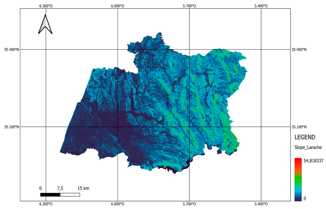
Figure 3.
Slope Derived from DEM of Larache Province (derived from SRTM DEM: NASA Shuttle Radar Topography Mission, processed and visualized in QGIS)
Figure 3.
Slope Derived from DEM of Larache Province (derived from SRTM DEM: NASA Shuttle Radar Topography Mission, processed and visualized in QGIS)
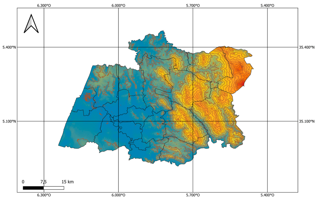
Figure 5.
Spatial distribution of cumulative rainfall (mm per 15-day interval) derived from CHIRPS for four consecutive periods (01-15 January, 16-30 January, 31 January-14 February, and 15-28 February 2026).
Figure 5.
Spatial distribution of cumulative rainfall (mm per 15-day interval) derived from CHIRPS for four consecutive periods (01-15 January, 16-30 January, 31 January-14 February, and 15-28 February 2026).
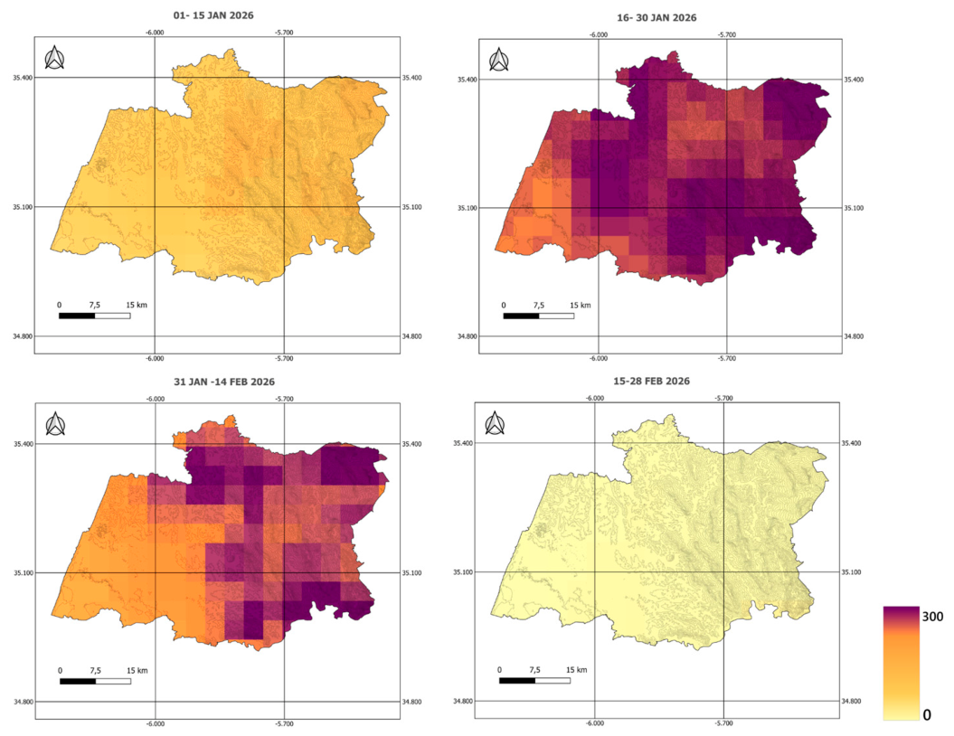
Figure 6.
CHIRPS daily rainfall time series and cumulative precipitation dynamics for the study period. The shaded area highlights the main rainfall event window (25 January-10 February 2026).
Figure 6.
CHIRPS daily rainfall time series and cumulative precipitation dynamics for the study period. The shaded area highlights the main rainfall event window (25 January-10 February 2026).
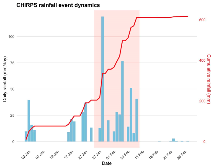
Figure 7.
Spatial distribution of VH backscatter anomaly. The map is dominated by near-zero values (light blue); slightly darker tones in the central-western sector indicate localized backscatter reduction potentially associated with surface water presence.
Figure 7.
Spatial distribution of VH backscatter anomaly. The map is dominated by near-zero values (light blue); slightly darker tones in the central-western sector indicate localized backscatter reduction potentially associated with surface water presence.
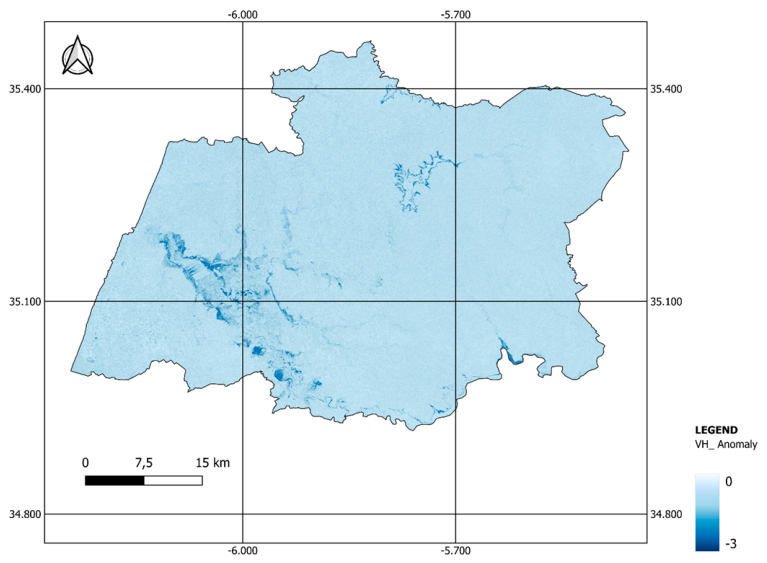
Figure 8.
VH z-score map. The predominantly light blue surface confirms general stability across the AOI; darker values concentrated along the central-western drainage corridor indicate statistically significant backscatter reductions associated with flood-affected areas.
Figure 8.
VH z-score map. The predominantly light blue surface confirms general stability across the AOI; darker values concentrated along the central-western drainage corridor indicate statistically significant backscatter reductions associated with flood-affected areas.
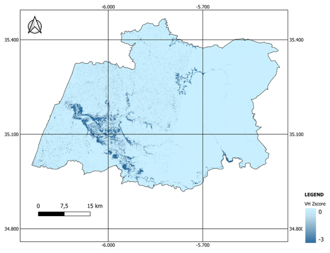
Figure 9.
Final SAR-derived flood extent based on VH anomaly and z-score thresholds, with spatial filtering and terrain masking applied. Flooded areas are delineated in blue.
Figure 9.
Final SAR-derived flood extent based on VH anomaly and z-score thresholds, with spatial filtering and terrain masking applied. Flooded areas are delineated in blue.
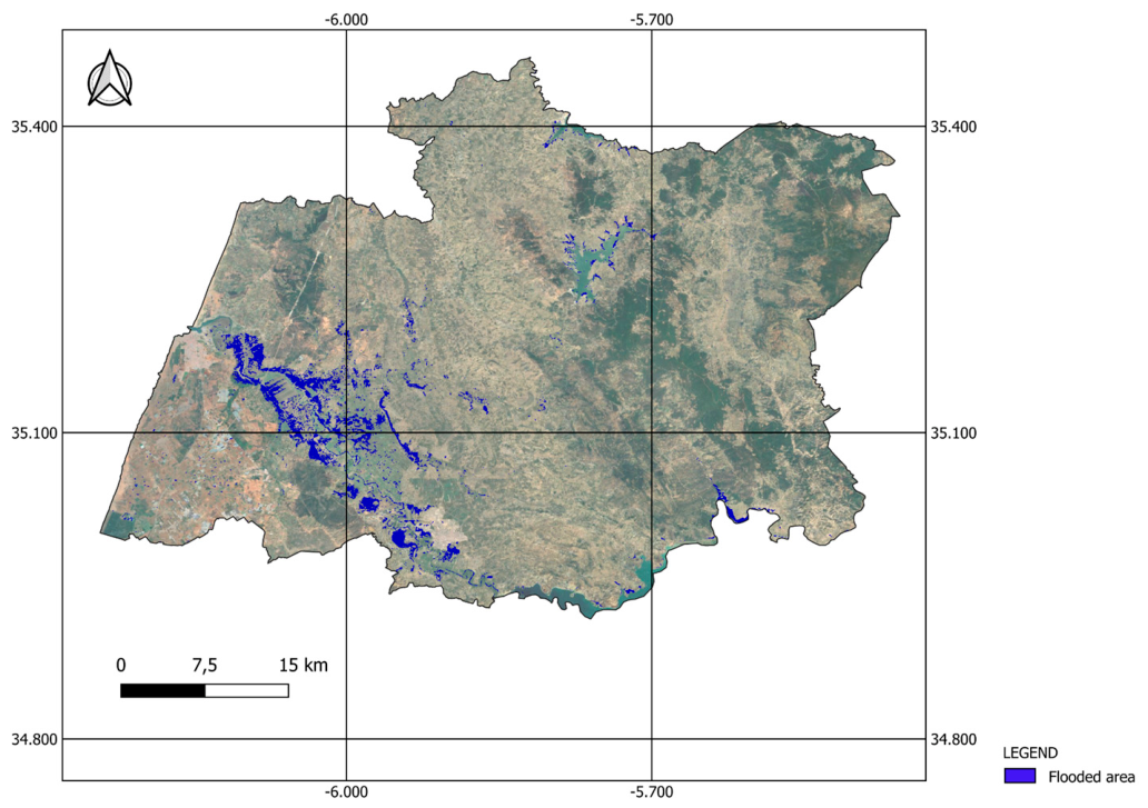
Figure 10.
Histogram of VH backscatter anomaly values with Otsu-derived threshold (red line). The distribution is strongly right-skewed; the sparse negative tail to the left of the threshold (−2.19) corresponds to flood-affected pixels characterized by significant backscatter reduction.
Figure 10.
Histogram of VH backscatter anomaly values with Otsu-derived threshold (red line). The distribution is strongly right-skewed; the sparse negative tail to the left of the threshold (−2.19) corresponds to flood-affected pixels characterized by significant backscatter reduction.
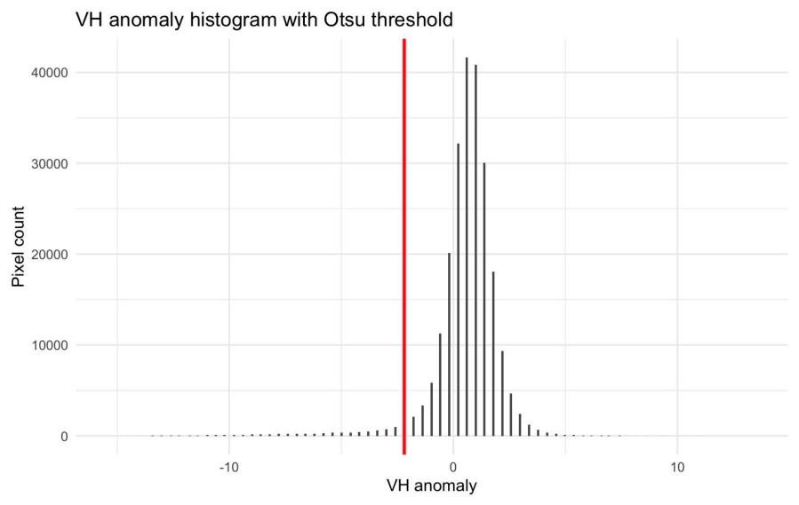
Figure 11.
Stability of the VH anomaly Otsu threshold under varying histogram parameter configurations (number of bins, minimum bucket width, and spatial scale).
Figure 11.
Stability of the VH anomaly Otsu threshold under varying histogram parameter configurations (number of bins, minimum bucket width, and spatial scale).
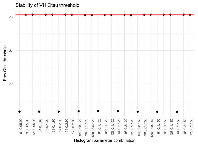
Figure 12.
Dynamic World land cover distribution within the SAR-derived flood mask across pre-event, post-event, spring 2025, and spring 2026 conditions, illustrating the temporal variability of surface classes and their response to flood dynamics.
Figure 12.
Dynamic World land cover distribution within the SAR-derived flood mask across pre-event, post-event, spring 2025, and spring 2026 conditions, illustrating the temporal variability of surface classes and their response to flood dynamics.
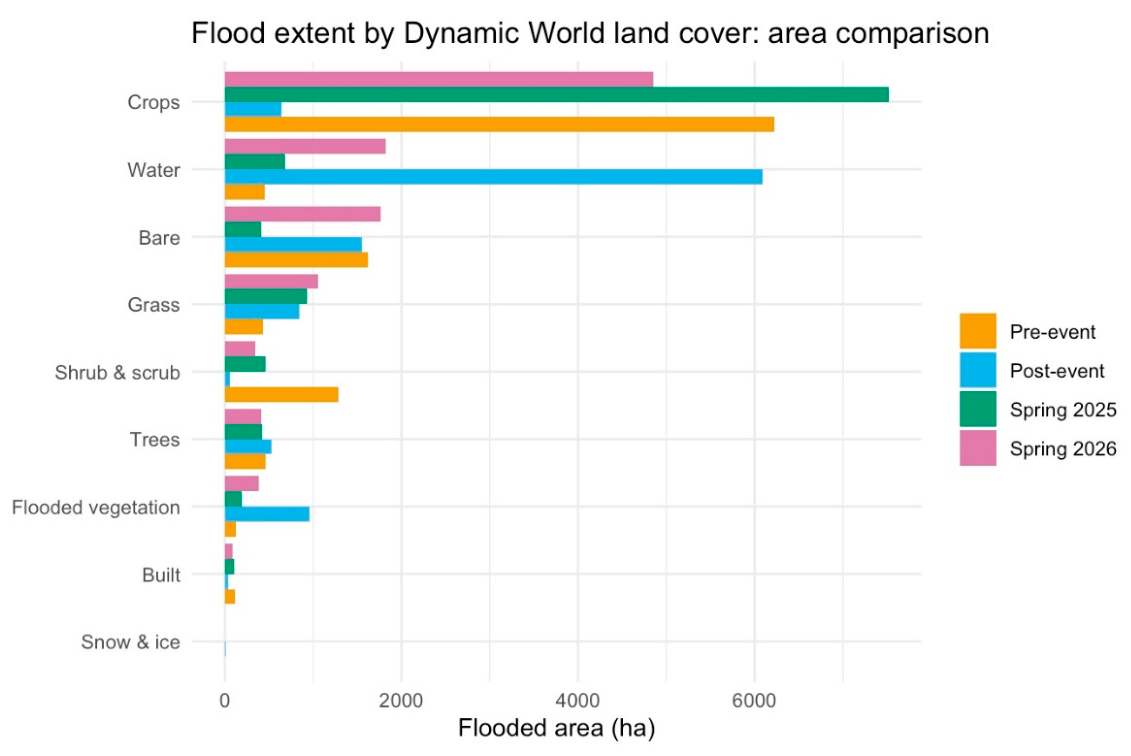
Figure 13.
Spatial distribution of the SAR-derived flood extent (blue) over the study area, with the 25 sample areas (Areas 1–25) delineated by red boxes for site-level land cover analysis.
Figure 13.
Spatial distribution of the SAR-derived flood extent (blue) over the study area, with the 25 sample areas (Areas 1–25) delineated by red boxes for site-level land cover analysis.
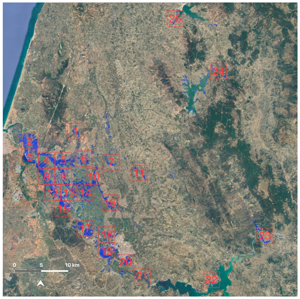
Figure 14.
(a) Land cover comparison across pre-event (Oct–Nov 2025), post-event (Jan–Feb 2026), spring 2025 (Mar–May 2025), and spring 2026 (Mar–May 2026) for sample Area 1 (centroid: 35.20°N, 6.00°W); (b) Dynamic Word Land Cover Classes Legend.
Figure 14.
(a) Land cover comparison across pre-event (Oct–Nov 2025), post-event (Jan–Feb 2026), spring 2025 (Mar–May 2025), and spring 2026 (Mar–May 2026) for sample Area 1 (centroid: 35.20°N, 6.00°W); (b) Dynamic Word Land Cover Classes Legend.
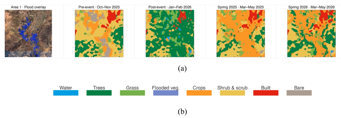
Figure 15.
Land cover comparison across pre-event (Oct–Nov 2025), post-event (Jan–Feb 2026), spring 2025 (Mar–May 2025), and spring 2026 (Mar–May 2026) for sample Area 2 (centroid: 35.18°N, 6.10°W).
Figure 15.
Land cover comparison across pre-event (Oct–Nov 2025), post-event (Jan–Feb 2026), spring 2025 (Mar–May 2025), and spring 2026 (Mar–May 2026) for sample Area 2 (centroid: 35.18°N, 6.10°W).

Figure 16.
Land cover comparison across pre-event (Oct–Nov 2025), post-event (Jan–Feb 2026), spring 2025 (Mar–May 2025), and spring 2026 (Mar–May 2026) for sample Area 3 (centroid: 35.16°N, 6.10°W).
Figure 16.
Land cover comparison across pre-event (Oct–Nov 2025), post-event (Jan–Feb 2026), spring 2025 (Mar–May 2025), and spring 2026 (Mar–May 2026) for sample Area 3 (centroid: 35.16°N, 6.10°W).

Figure 17.
Land cover comparison across pre-event (Oct–Nov 2025), post-event (Jan–Feb 2026), spring 2025 (Mar–May 2025), and spring 2026 (Mar–May 2026) for sample Area 4 (centroid: 35.15°N, 6.06°W).
Figure 17.
Land cover comparison across pre-event (Oct–Nov 2025), post-event (Jan–Feb 2026), spring 2025 (Mar–May 2025), and spring 2026 (Mar–May 2026) for sample Area 4 (centroid: 35.15°N, 6.06°W).

Figure 18.
Land cover comparison across pre-event (Oct–Nov 2025), post-event (Jan–Feb 2026), spring 2025 (Mar–May 2025), and spring 2026 (Mar–May 2026) for sample Area 5 (centroid: 35.15°N, 6.03°W).
Figure 18.
Land cover comparison across pre-event (Oct–Nov 2025), post-event (Jan–Feb 2026), spring 2025 (Mar–May 2025), and spring 2026 (Mar–May 2026) for sample Area 5 (centroid: 35.15°N, 6.03°W).

Figure 19.
Land cover comparison across pre-event (Oct–Nov 2025), post-event (Jan–Feb 2026), spring 2025 (Mar–May 2025), and spring 2026 (Mar–May 2026) for sample Area 6 (centroid: 35.15°N, 5.99°W).
Figure 19.
Land cover comparison across pre-event (Oct–Nov 2025), post-event (Jan–Feb 2026), spring 2025 (Mar–May 2025), and spring 2026 (Mar–May 2026) for sample Area 6 (centroid: 35.15°N, 5.99°W).

Figure 20.
Land cover comparison across pre-event (Oct–Nov 2025), post-event (Jan–Feb 2026), spring 2025 (Mar–May 2025), and spring 2026 (Mar–May 2026) for sample Area 7 (centroid: 35.15°N, 5.93°W).
Figure 20.
Land cover comparison across pre-event (Oct–Nov 2025), post-event (Jan–Feb 2026), spring 2025 (Mar–May 2025), and spring 2026 (Mar–May 2026) for sample Area 7 (centroid: 35.15°N, 5.93°W).

Figure 21.
Land cover comparison across pre-event (Oct–Nov 2025), post-event (Jan–Feb 2026), spring 2025 (Mar–May 2025), and spring 2026 (Mar–May 2026) for sample Area 8 (centroid: 35.12°N, 6.06°W).
Figure 21.
Land cover comparison across pre-event (Oct–Nov 2025), post-event (Jan–Feb 2026), spring 2025 (Mar–May 2025), and spring 2026 (Mar–May 2026) for sample Area 8 (centroid: 35.12°N, 6.06°W).

Figure 22.
Land cover comparison across pre-event (Oct–Nov 2025), post-event (Jan–Feb 2026), spring 2025 (Mar–May 2025), and spring 2026 (Mar–May 2026) for sample Area 9 (centroid: 35.12°N, 6.03°W).
Figure 22.
Land cover comparison across pre-event (Oct–Nov 2025), post-event (Jan–Feb 2026), spring 2025 (Mar–May 2025), and spring 2026 (Mar–May 2026) for sample Area 9 (centroid: 35.12°N, 6.03°W).

Figure 23.
Land cover comparison across pre-event (Oct–Nov 2025), post-event (Jan–Feb 2026), spring 2025 (Mar–May 2025), and spring 2026 (Mar–May 2026) for sample Area 10 (centroid: 35.12°N, 5.97°W).
Figure 23.
Land cover comparison across pre-event (Oct–Nov 2025), post-event (Jan–Feb 2026), spring 2025 (Mar–May 2025), and spring 2026 (Mar–May 2026) for sample Area 10 (centroid: 35.12°N, 5.97°W).

Figure 24.
Land cover comparison across pre-event (Oct–Nov 2025), post-event (Jan–Feb 2026), spring 2025 (Mar–May 2025), and spring 2026 (Mar–May 2026) for sample Area 11 (centroid: 35.13°N, 5.87°W).
Figure 24.
Land cover comparison across pre-event (Oct–Nov 2025), post-event (Jan–Feb 2026), spring 2025 (Mar–May 2025), and spring 2026 (Mar–May 2026) for sample Area 11 (centroid: 35.13°N, 5.87°W).

Figure 25.
Land cover comparison across pre-event (Oct–Nov 2025), post-event (Jan–Feb 2026), spring 2025 (Mar–May 2025), and spring 2026 (Mar–May 2026) for sample Area 12 (centroid: 35.10°N, 6.05°W).
Figure 25.
Land cover comparison across pre-event (Oct–Nov 2025), post-event (Jan–Feb 2026), spring 2025 (Mar–May 2025), and spring 2026 (Mar–May 2026) for sample Area 12 (centroid: 35.10°N, 6.05°W).

Figure 26.
Land cover comparison across pre-event (Oct–Nov 2025), post-event (Jan–Feb 2026), spring 2025 (Mar–May 2025), and spring 2026 (Mar–May 2026) for sample Area 13 (centroid: 35.10°N, 6.02°W).
Figure 26.
Land cover comparison across pre-event (Oct–Nov 2025), post-event (Jan–Feb 2026), spring 2025 (Mar–May 2025), and spring 2026 (Mar–May 2026) for sample Area 13 (centroid: 35.10°N, 6.02°W).

Figure 27.
Land cover comparison across pre-event (Oct–Nov 2025), post-event (Jan–Feb 2026), spring 2025 (Mar–May 2025), and spring 2026 (Mar–May 2026) for sample Area 14 (centroid: 35.10°N, 5.98°W).
Figure 27.
Land cover comparison across pre-event (Oct–Nov 2025), post-event (Jan–Feb 2026), spring 2025 (Mar–May 2025), and spring 2026 (Mar–May 2026) for sample Area 14 (centroid: 35.10°N, 5.98°W).

Figure 28.
Land cover comparison across pre-event (Oct–Nov 2025), post-event (Jan–Feb 2026), spring 2025 (Mar–May 2025), and spring 2026 (Mar–May 2026) for sample Area 15 (centroid: 35.07°N, 6.03°W).
Figure 28.
Land cover comparison across pre-event (Oct–Nov 2025), post-event (Jan–Feb 2026), spring 2025 (Mar–May 2025), and spring 2026 (Mar–May 2026) for sample Area 15 (centroid: 35.07°N, 6.03°W).

Figure 29.
Land cover comparison across pre-event (Oct–Nov 2025), post-event (Jan–Feb 2026), spring 2025 (Mar–May 2025), and spring 2026 (Mar–May 2026) for sample Area 16 (centroid: 35.08°N, 5.93°W).
Figure 29.
Land cover comparison across pre-event (Oct–Nov 2025), post-event (Jan–Feb 2026), spring 2025 (Mar–May 2025), and spring 2026 (Mar–May 2026) for sample Area 16 (centroid: 35.08°N, 5.93°W).

Figure 30.
Land cover comparison across pre-event (Oct–Nov 2025), post-event (Jan–Feb 2026), spring 2025 (Mar–May 2025), and spring 2026 (Mar–May 2026) for sample Area 17 (centroid: 35.04°N, 5.98°W).
Figure 30.
Land cover comparison across pre-event (Oct–Nov 2025), post-event (Jan–Feb 2026), spring 2025 (Mar–May 2025), and spring 2026 (Mar–May 2026) for sample Area 17 (centroid: 35.04°N, 5.98°W).

Figure 31.
Land cover comparison across pre-event (Oct–Nov 2025), post-event (Jan–Feb 2026), spring 2025 (Mar–May 2025), and spring 2026 (Mar–May 2026) for sample Area 18 (centroid: 35.03°N, 5.94°W).
Figure 31.
Land cover comparison across pre-event (Oct–Nov 2025), post-event (Jan–Feb 2026), spring 2025 (Mar–May 2025), and spring 2026 (Mar–May 2026) for sample Area 18 (centroid: 35.03°N, 5.94°W).

Figure 32.
Land cover comparison across pre-event (Oct–Nov 2025), post-event (Jan–Feb 2026), spring 2025 (Mar–May 2025), and spring 2026 (Mar–May 2026) for sample Area 19 (centroid: 35.00°N, 5.94°W).
Figure 32.
Land cover comparison across pre-event (Oct–Nov 2025), post-event (Jan–Feb 2026), spring 2025 (Mar–May 2025), and spring 2026 (Mar–May 2026) for sample Area 19 (centroid: 35.00°N, 5.94°W).

Figure 33.
Land cover comparison across pre-event (Oct–Nov 2025), post-event (Jan–Feb 2026), spring 2025 (Mar–May 2025), and spring 2026 (Mar–May 2026) for sample Area 20 (centroid: 34.98°N, 5.90°W).
Figure 33.
Land cover comparison across pre-event (Oct–Nov 2025), post-event (Jan–Feb 2026), spring 2025 (Mar–May 2025), and spring 2026 (Mar–May 2026) for sample Area 20 (centroid: 34.98°N, 5.90°W).

Figure 34.
Land cover comparison across pre-event (Oct–Nov 2025), post-event (Jan–Feb 2026), spring 2025 (Mar–May 2025), and spring 2026 (Mar–May 2026) for sample Area 21 (centroid: 34.96°N, 5.87°W).
Figure 34.
Land cover comparison across pre-event (Oct–Nov 2025), post-event (Jan–Feb 2026), spring 2025 (Mar–May 2025), and spring 2026 (Mar–May 2026) for sample Area 21 (centroid: 34.96°N, 5.87°W).

Figure 35.
Land cover comparison across pre-event (Oct–Nov 2025), post-event (Jan–Feb 2026), spring 2025 (Mar–May 2025), and spring 2026 (Mar–May 2026) for sample Area 22 (centroid: 34.95°N, 5.73°W).
Figure 35.
Land cover comparison across pre-event (Oct–Nov 2025), post-event (Jan–Feb 2026), spring 2025 (Mar–May 2025), and spring 2026 (Mar–May 2026) for sample Area 22 (centroid: 34.95°N, 5.73°W).

Figure 36.
Land cover comparison across pre-event (Oct–Nov 2025), post-event (Jan–Feb 2026), spring 2025 (Mar–May 2025), and spring 2026 (Mar–May 2026) for sample Area 23 (centroid: 35.02°N, 5.62°W).
Figure 36.
Land cover comparison across pre-event (Oct–Nov 2025), post-event (Jan–Feb 2026), spring 2025 (Mar–May 2025), and spring 2026 (Mar–May 2026) for sample Area 23 (centroid: 35.02°N, 5.62°W).

Figure 37.
Land cover comparison across pre-event (Oct–Nov 2025), post-event (Jan–Feb 2026), spring 2025 (Mar–May 2025), and spring 2026 (Mar–May 2026) for sample Area 24 (centroid: 35.30°N, 5.71°W).
Figure 37.
Land cover comparison across pre-event (Oct–Nov 2025), post-event (Jan–Feb 2026), spring 2025 (Mar–May 2025), and spring 2026 (Mar–May 2026) for sample Area 24 (centroid: 35.30°N, 5.71°W).

Figure 38.
Land cover comparison across pre-event (Oct–Nov 2025), post-event (Jan–Feb 2026), spring 2025 (Mar–May 2025), and spring 2026 (Mar–May 2026) for sample Area 25 (centroid: 35.39°N, 5.80°W).
Figure 38.
Land cover comparison across pre-event (Oct–Nov 2025), post-event (Jan–Feb 2026), spring 2025 (Mar–May 2025), and spring 2026 (Mar–May 2026) for sample Area 25 (centroid: 35.39°N, 5.80°W).

Figure 39.
Multi-temporal Dynamic World land cover fractions (%) across 25 sample areas for four temporal windows: spring 2025 (Mar–May 2025), pre-event (Oct–Nov 2025), post-event (Jan–Feb 2026), and spring 2026 (Mar–May 2026). Panel (a) shows the combined water and flooded vegetation fraction as a proxy for flood signal intensity (colour scale 0–70%); panel (b) shows crop cover (0–100%); panel (c) shows bare soil fraction (0–50%). Cell values represent mode-aggregated land cover percentages derived from the Dynamic World V1 dataset at 10 m resolution. Area numbers correspond to the sample locations shown in Figure 13.
Figure 39.
Multi-temporal Dynamic World land cover fractions (%) across 25 sample areas for four temporal windows: spring 2025 (Mar–May 2025), pre-event (Oct–Nov 2025), post-event (Jan–Feb 2026), and spring 2026 (Mar–May 2026). Panel (a) shows the combined water and flooded vegetation fraction as a proxy for flood signal intensity (colour scale 0–70%); panel (b) shows crop cover (0–100%); panel (c) shows bare soil fraction (0–50%). Cell values represent mode-aggregated land cover percentages derived from the Dynamic World V1 dataset at 10 m resolution. Area numbers correspond to the sample locations shown in Figure 13.
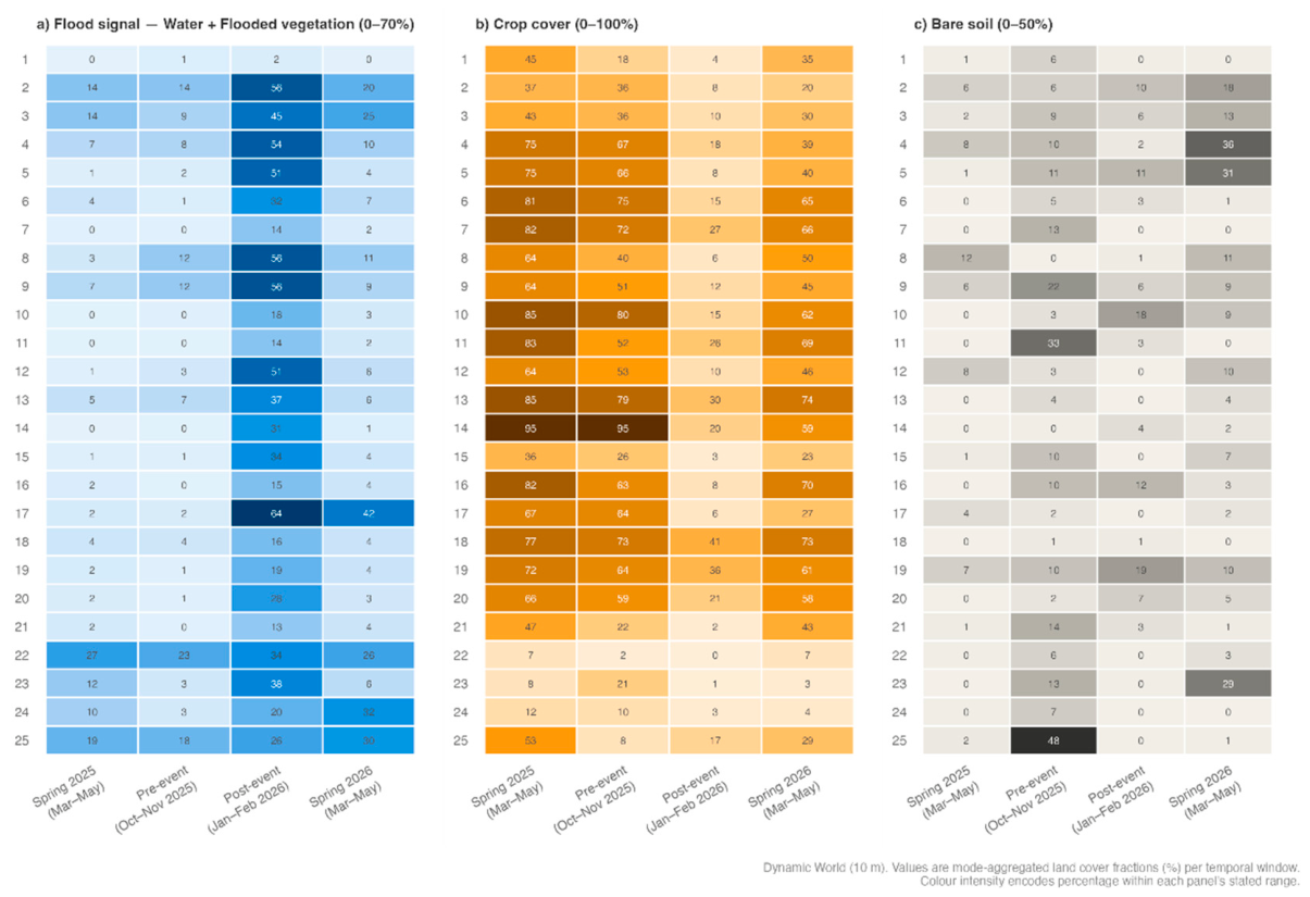

Table 1.
Rainfall statistics for 15-day intervals derived from CHIRPS over the study area. Minimum (Min), maximum (Max), mean (Mean), and 95th percentile (P95) precipitation values are reported for each period (mm per 15-day interval).
Table 1.
Rainfall statistics for 15-day intervals derived from CHIRPS over the study area. Minimum (Min), maximum (Max), mean (Mean), and 95th percentile (P95) precipitation values are reported for each period (mm per 15-day interval).
| Period | Min (mm) | Max (mm) | Mean (mm) | P95 (mm) |
|---|---|---|---|---|
| 01-15 Jan 2026 | 54.84 | 97.77 | 76.42 | 91.64 |
| 16-30 Jan 2026 | 234.94 | 352.76 | 283.50 | 321.71 |
| 31 Jan-14 Feb 2026 | 145.83 | 367.28 | 255.92 | 310.23 |
| 15-28 Feb 2026 | 2.73 | 18.95 | 5.02 | 7.17 |
Table 2.
Dynamic World land cover distribution within the SAR-derived flood mask under pre-event conditions. Percentages are computed relative to the flooded area.
Table 2.
Dynamic World land cover distribution within the SAR-derived flood mask under pre-event conditions. Percentages are computed relative to the flooded area.
| Pre-event Land cover class | Area (ha) | Percentage (%) |
|---|---|---|
| Crops | 6224.1208 | 58.06 |
| Bare | 1624.1234 | 15.15 |
| Shrub & scrub | 1284.0742 | 11.97 |
| Trees | 463.0624 | 4.32 |
| Water | 453.9467 | 4.23 |
| Grass | 428.2804 | 3.99 |
| Flooded vegetation | 126.2800 | 1.17 |
| Built | 115.1500 | 1.07 |
Table 3.
Dynamic World land cover distribution within the SAR-derived flood mask during post-event conditions, highlighting the increase in water and flooded vegetation classes.
Table 3.
Dynamic World land cover distribution within the SAR-derived flood mask during post-event conditions, highlighting the increase in water and flooded vegetation classes.
| Post-event Land cover class | Area (ha) | Percentage (%) |
|---|---|---|
| Water | 6088.8329 | 56.80 |
| Bare | 1557.0869 | 14.52 |
| 959.5018 | 8.95 | |
| Grass | 839.1193 | 7.82 |
| Crops | 645.1473 | 6.01 |
| Trees | 524.6238 | 4.89 |
| Shrub & scrub | 58.8047 | 0.54 |
| Built | 41.0011 | 0.38 |
| Snow & ice | 4.9200 | 0.04 |
Table 4.
Dynamic World land cover distribution within the SAR-derived flood mask for the 2025 spring growing season, representing typical seasonal land cover conditions.
Table 4.
Dynamic World land cover distribution within the SAR-derived flood mask for the 2025 spring growing season, representing typical seasonal land cover conditions.
| Spring growing season (2025) Land cover class | Area (ha) | Percentage (%) |
|---|---|---|
| Crops | 7514.6675 | 70.10 |
| Grass | 932.2757 | 8.69 |
| Water | 678.7754 | 6.33 |
| Shrub & scrub | 458.5092 | 4.27 |
| Trees | 424.6456 | 3.96 |
| Bare | 412.0344 | 3.84 |
| Flooded vegetation | 195.0700 | 1.81 |
| Built | 103.0600 | 0.96 |
Table 5.
Dynamic World land cover distribution within the SAR-derived flood mask for the 2026 spring growing season. Comparison with Table 4 reflects post-flood land cover recovery and persistent surface changes relative to the 2025 seasonal baseline.
Table 5.
Dynamic World land cover distribution within the SAR-derived flood mask for the 2026 spring growing season. Comparison with Table 4 reflects post-flood land cover recovery and persistent surface changes relative to the 2025 seasonal baseline.
| Spring growing season (2026) Land cover class | Area (ha) | Percentage (%) |
|---|---|---|
| Crops | 4854.0 | 45.28 |
| Grass | 1052.1 | 9.82 |
| Water | 1823.4 | 17.01 |
| Shrub & scrub | 341.8 | 3.19 |
| Trees | 408.3 | 3.81 |
| Bare | 1763.1 | 16.45 |
| Flooded vegetation | 387.9 | 3.62 |
| Built | 88.5 | 0.83 |
Disclaimer/Publisher’s Note: The statements, opinions and data contained in all publications are solely those of the individual author(s) and contributor(s) and not of MDPI and/or the editor(s). MDPI and/or the editor(s) disclaim responsibility for any injury to people or property resulting from any ideas, methods, instructions or products referred to in the content. |
© 2026 by the authors. Licensee MDPI, Basel, Switzerland. This article is an open access article distributed under the terms and conditions of the Creative Commons Attribution (CC BY) license (http://creativecommons.org/licenses/by/4.0/).
Copyright: This open access article is published under a Creative Commons CC BY 4.0 license, which permit the free download, distribution, and reuse, provided that the author and preprint are cited in any reuse.