

Submitted:
29 June 2026
Posted:
30 June 2026
You are already at the latest version
Abstract
Obesity is a major problem worldwide, particularly in Latin countries such as Mexico, Peru and Colombia. This study aims to evaluate five models (XGBoost, Random Forest, Multinomial Logistic Regression, Linear Discriminant Analysis (LDA) and Support Vector Machines (SVM)) from the statistical and machine learning fields to determine which of them is the most effective in classification of obesity levels in a multivariate classification model. The research uses a dataset of 2111 records consisting of 17 physiological and behavioral attributes which had to be preprocessed, such as one-hot encoding and multicollinearity filtering, and a powerful 10-fold cross validation methodology. It is shown that the results of ensemble methods are much better than those of the traditional parametric ones. XGBoost achieved the highest classification accuracy (97.54%), and an F_1-score of 0.9747, while Random Forest achieved the 2nd highest classification accuracy (95.64%). For all comparisons, McNemar's pairwise significance tests validated the superiority of XGBoost (with p<0.0001). Feature importance analysis was used to determine the most significant features as follows: weight, height, age and number of vegetables consumed per week (FCVC). While the study showcases the power of gradient boosting for capturing non-linear interactions in health data, the exclusive use of synthetic data (77% from SMOTE) poses drawbacks as it may overestimate performance and limit generalizability. The proposed ensemble architectures should be further evaluated on larger, all-nonsynthetic datasets to be clinically generalizable in the future.
Keywords:
obesity classification
; statistical learning
; ensemble methods
; machine learning
; XGBoost (eXtreme gradient boosting)
; random forest
; SMOTE (Synthetic Minority Over-sampling Technique)
; multivariate health data
; cross validation
1. Introduction
Obesity is a major health problem in the world and is strongly associated with chronic diseases like type 2 diabetes, cardiovascular diseases and various forms of cancer. Over the past decades, there has been a significant increase in obesity rates in some Latin American countries, including Mexico, Peru and Colombia, which is due to the changes in their dietary habits and increased sedentary lifestyle.
The primary research question in this study is to determine the best statistical learning model for accurately and robustly classify obesity level and efficiency of modern ensemble methods compared to the traditional statistical methods.
This study employs a dataset that was collected and published by [6] and made publicly available by the UCI Machine Learning Repository (UCIMLR) [9]. It has 2111 records, and 17 attributes. The variable to be classified is the categorization NObeyesdad with 7 categories: Insufficient Weight, Obesity Type I, Obesity Type II, Obesity Type III. The 23% medical data is collected directly from users via a web platform in Mexico, Peru and Colombia, as data of this scale and balance is not easy to obtain, the remaining 77% was synthetically generated using the Weka SMOTE (Synthetic Minority Over-sampling Technique) filter to balance the classes.
2. Related Works
Machine learning methods have increasingly been found useful in recent years in healthcare, particularly for predictive modeling and risk classification. It has been shown previously that algorithms like Random Forests and Support Vector Machines (SVM) have generally better performance in classification problems with complex, non-linear relationships than traditional statistical methods [1,2]. Random Forest can be used to deal with variance and overfitting by performing bootstrap aggregating, whereas SVM can be used to optimize classification by finding hyperplanes in high dimensional spaces. In some cases multi-class health data is noisy and highly imbalanced and SVMs may not work on such data.
Concerning obesity prediction, [5] found that the ensemble models had the highest accuracy of 89.68%, as they were able to capture the complicated relationships between different types of lifestyle factors. Similarly, [3] showed that structured tabular data generally performs well with gradient boosting models like XGBoost, which improve iteratively by decreasing the error of classification, compared to single-model methods, while also showing higher accuracy and robustness.
A solution to the issue of class imbalance still needs to be developed for these medical datasets. One such technique that has been widely adopted is the Synthetic Minority Over-sampling Technique (SMOTE) [4] which has been widely used to improve the classification accuracy by generating synthetic observations in the minority classes.
There is, however, limited of literature available which studies these predictive models independently or critically investigates the interaction between class imbalance techniques and model selection. To address this, the study will compare five models systematically in the same stringent cross validation setting, which are parametric and non-parametric models, and select the best model architecture for the multivariate obesity classification.
3. Methods
3.1. Data and Preprocessing
There are 17 attributes, and 2111 participants in the data. The population is highly balanced by gender, consisting of 1,043 females (49.4%) and 1,068 males (50.6%). The attributes are continuous variables such as the Age, Height, Weight, and categorical variables, which are related to lifestyle choices, for example, the Frequency of Consumption of Vegetables [FCVC], Number of main Meals [NCP] or the Physical activity Frequency [FAF].
There were several pre-processing steps preceeding the training of the models. One-hot encoding with no reference category dropped and with the option fullRank = TRUE in the dummyVars function from the caret package, was used to encode categorical predictor variables, with no intention of dropping any variables to prevent multicollinearity. Second, the predictors showing a negligible variance were identified and dropped from the dataset with the function nearZeroVar which identifies predictors with insufficient discriminatory information. Third, the features that were highly collinear (i.e. with correlation between the two features greater than 0.95) were removed using a Pearson correlation filter. The last feature matrix was filtered and then standardized within the folds, without leakage data into the folds by only using the statistics for the training fold in each fold.
3.2. Statistical and Machine Learning Methods
Five machine learning algorithms were developed to classify obesity level. Each model was chosen to give a range of comparative baseline models from the rigid parametric assumption through to the very flexible non-linear mapping. Suppose that is the standardized feature vector for a particular observation and that is the number of classes of obesity.
XGBoost (eXtreme Gradient Boosting)
XGBoost trains a collection of T regression trees to minimize the following cost function: a differentiable loss function over all N training data points, added to a regularization term on the complexity of all the trees [3]:
where is the multiclass log-loss (mlogloss), is the number of leaves in tree t, is the vector of leaf weights, and , are regularization constants. The ensemble prediction is the sum of all tree outputs:
Class membership is recovered via the multi:softmax objective. Hyperparameters: max_depth = 6, eta = 0.1, nrounds = 100.
Assumptions: The observations are independent of each other. There are no distributional assumptions for the predictors. Features can have arbitrary non-linear relationships with the outcome. The following trees are scaled to the negative gradient The (pseudo-residuals) of the loss with respect to the current ensemble prediction.
Random Forest
Random Forest is a combination of B classification trees, where each tree is built on a random subset of the training data (bootstrap sample) [1]. The final class prediction is the one with the largest number of votes:
where is the class predicted by the b-th tree. At each node split, only a random subset of features is considered, reducing tree correlation. Node purity is measured by the Gini impurity:
where is the proportion of class-k observations at the node. Hyperparameters: ntree = 500, mtry = .
Assumptions: Observations are independent. No distributional assumptions are placed on the predictors. Enough trees are provided if there are enough trees for the shelter they require. is obliged to bring the variability of the vote to a standstill; by the law of large numbers, it is guaranteed that convergence of the ensemble error as .
Multinomial Logistic Regression
Multinomial logistic regression models the conditional probability of class k as a softmax function of linear combination of the predictors:
where is the coefficient vector for class k. Parameters are estimated by maximizing the penalized log-likelihood with weight decay regularization ():
Assumptions: (1) Independence of irrelevant alternatives (IIA): The log-odds for any two classes are independent of the other classes. (2) Linear in the log-odds: The log-odds are a Function that is linear in . (3) Observations are independent. (4) No perfect multicollinearity among predictors. These assumptions are frequently not met by High dimensional, non-normally distributed health data.
Linear Discriminant Analysis (LDA)
LDA uses linear combinations of the features to maximally separate the K classes. Using the class conditional densities that are Gaussian, with a common covariance matrix , Bayes’ theorem yields the linear discriminant function:
where is the class-k mean vector, is the class prior, and is the pooled within-class covariance matrix, estimated as:
An observation is assigned to the class .
Assumptions: (1) Multivariate normality: the predictors Class data are assumed to be normally distributed (multivariate Gaussian distribution) within each class. (2) Homoscedasticity: the covariance matrix is the same for each of the K classes, . (3) Observations are independent. Violations of assumptions (1) and (2) - both expected in real-world health data - directly inflate classification error.
Support Vector Machine (SVM) with RBF Kernel
The SVM looks for the hyperplane with the largest margin in the feature space induced by the kernel. It is a solution to the following equation in the soft-margin formulation:
where is the mapping of the inputs to a higher-dimensional Hilbert space, while C is the regularization parameter, where cost = 1 and is a slack variable for soft-margin constraints. The inner product in feature space is implicit in the radial basis function (RBF) kernel:
where controls the width of the Gaussian kernel. Multi-class classification using one-vs-one (OVO) decomposition, fitting binary classifiers and assigning each observation to the class with the most votes.
Assumptions: (1) No parametric distributional form is assumed for the predictors. (2) The margin-maximization principle requires that the classes be separable, if not in a soft-margin sense, in the space induced by the kernel. (3) Observations are independent. (4) The RBF kernel assumes implicitly smooth class boundaries and locally Euclidean class structures, which may be problematic when classes are very overlapping in the original feature space.
3.3. Model Evaluation
All models were tested in 10-fold cross validation framework for out-of-sample reliability and to prevent over fitting. The dataset was split into stratified folds, with each fold k used for test set and the rest used for train set. The mean and standard deviation were used as standardization parameters only in the training folds, and not in the held out fold, thus avoiding data leakage.
The performance was quantitatively measured using four macro-averaged metrics calculated by averaging across the obesity classes. Assume that there are k classes and that the true positive rates, false positive rates and false negative rates are denoted by respectively.
McNemar’s test [7] was used to determine the statistical significance of any pair-wise differences in performances. If b is the number of cases that are classified as disagreements between the best model and the alternative model and c is the number of cases that are classified as disagreements between the alternative model and the best model, then the test statistic with continuity correction is:
which is distributed as a with one degree of freedom under the null hypothesis of equal error rates. The significance level used was set as .
4. Results
4.1. Descriptive Summaries and Feature Analysis
The distribution of the data is very uniform within each of the seven obesity groups. As seen in Figure 1, the populations were split into five classifications, ranging from 12.9% to 16.6% of the total population.
Table 1 provides a descriptive summary of the primary physical attributes stratified by gender. While the mean age is similar between females (, ) and males (, ), males in the dataset present with higher average height and weight. Notably, the weight variance for females () is substantially higher than for males (), indicating a wider spread of extreme weight values in the female cohort.
The feature importance analysis based on Gini impurity (see Figure 2) shows that Weight and Height have the highest Gini scores of 560.8 and 166.7, respectively, suggesting that they are the most prominent features in the classification process. There are also high predictive importance for certain other variables, such as Age (150.3) and FCVC (vegetable consumption, 142.7). The strong signal of lifestyle factors (FCVC) proves that obesity classification is not solely based on the anthropometric values.
The separability of obesity classes in a reduced dimensional space was evaluated by a principal component analysis (PCA) on the standardized feature matrix (Figure 3). Together, the first two principal components explain 31.7% of the total variance, with the first principal component accounting for 19.0%, and the second for 12.7%. The resulting biplot shows largely separate clusters for the seven obesity categories, and the separation between Insufficient Weight and the higher levels of Obesity are clearly seen, which is consistent with the feature importance results displayed in Figure 2 showing that Weight is the most dominant feature.
4.2. Model Performance
The results of 10-fold cross validation are summarized in Table 2. XGBoost achieved the highest performance across all metrics, with an accuracy of 97.54% and an F1-Score of 0.9747. Random Forest was very close behind with an accuracy of 95.64%. The results in Figure 4 show that XGBoost was consistent across all 10 folds.
The confusion matrix for Figure 4 is shown in Table 3. They obtained a highly accurate classification with the XGBoost model, achieving an overall accuracy of 97.54%. The most common misclassifications are between the neighboring weight categories (e.g. Normal Weight and Overweight Level I), which is physiologically predictable because the boundaries between weight categories are continuous. The pairwise significance tests using McNemar’s method showed that XGBoost’s superiority is statistically significant when compared to all other models being analysed (;Table 4).
Interpretation: These two models, XGBoost and Random Forest, have shown to be more effective compared to other models, highlighting that obesity indicators are very non-linear. The complex real-world interactions between the physical and lifestyle variables made the classic models, such as LDA, which have strict parametric assumptions (that is, equal covariance matrices for the seven obesity classes) inadequate. The iterative corrections made by the previous trees in XGBoost helped the algorithm be better able to capture these complex interactions between features than SVM or Logistic Regression.
5. Discussion
The results show that ensemble learning methods such as XGBoost gave a very accurate prediction of obesity level. Both of these predictors (Weight and Height) are important in defining body mass, confirming the central role of these measures in any good obesity classification system, and the contribution of the six other lifestyle variables (such as Frequency of consumption of vegetables (FCVC)) reinforces the need to include the behavioral context in any sound obesity classification system.
The results obtained from this methodological approach indicate that classical statistical models may not be suitable for high-dimensional health data, given its non-normal distribution. It is better to go with ensemble approaches as they can be more flexible in their structure and don’t require any distributional assumptions.
Limitations and Bias: The accuracy of the study is very high (97.54%), but the disadvantage is the high percentage of synthetic data used in this work. The machine learning models have the potential to have learned fake distribution structures instead of real-world variance in the dataset, since 77% of the dataset was created using SMOTE before the evaluation stage. Due to their tightly clustered and unnatural patterns, synthetic oversampled data can be exploited by models such as XGBoost. As a result, these very good performance ratings are likely to be over-optimistic and have serious external validity issues. It is likely to be much less accurate in the real world, using a non-synthetic patient population. In addition, the sample size is limited to three Latin American countries (Mexico, Peru, Colombia) and results may not be applicable to other countries and communities in Latin American countries regarding dietary patterns and healthcare systems.
Implications and Future Work: Although there are limitations on the synthetic data, the results are applicable to public health. Basic physical features can be used together with behavioural survey data in a gradient boosting model, which have the potential to accurately predict the obesity stage and to prevent clinical interventions at higher risk of obesity stages. Future studies could use the following directions: (1) expanding the authentic, non-synthetic component of the data set by using ongoing data collection via web platforms, to validate the effectiveness of the ensemble models in predicting real populations; (2) using post-hoc interpretability methods such as SHAP (SHapley Additive exPlanations) values to generate clinically-actionable feature-level explanations of individual predictions; (3) testing model performance in external, geographically-distributed validation cohorts, to assess cross-cultural generalizability; and (4) investigating other ensemble methods such as stacking or voting classifiers, and determining their performance and whether further accuracy gains are achievable beyond XGBoost.
AI Tools Disclosure: This manuscript was not prepared with the aid of AI writing or language tools. The authors shall be solely responsible for any errors of fact or omissions in or resulting from the use of this information.
Author Contributions
All authors contributed equally to the Introduction, Preliminaries, Main results, and drafting of this work. All authors have read and agreed to the published version of the manuscript.
Data Availability Statement
The data for this paper are publicly available at https://archive.ics.uci.edu/dataset/544/estimation+of+obesity+levels+based+on+eating+habits+and+physical+condition under an open-source license.
Conflicts of Interest
The authors declare no conflicts of interest.
References
- Breiman, L. Random forests. Mach. Learn. 2001, 45(1), 5–32. [Google Scholar] [CrossRef]
- Cortes, C.; Vapnik, V. Support-vector networks. Mach. Learn. 1995, 20(3), 273–297. [Google Scholar] [CrossRef]
- Chen, T.; Guestrin, C. XGBoost: A scalable tree boosting system. In Proceedings of the 22nd ACM SIGKDD International Conference on Knowledge Discovery and Data Mining, 2016; pp. 785–794. [Google Scholar]
- Chawla, N. V.; Bowyer, K. W.; Hall, L. O.; Kegelmeyer, W. P. SMOTE: Synthetic minority over-sampling technique. J. Artif. Intell. Res. 2002, 16, 321–357. [Google Scholar] [CrossRef]
- indal, K.; Baliyan, N.; Rana, P. S. Obesity prediction using ensemble machine learning approaches. In Recent Findings in Intelligent Computing Techniques: Proceedings of the 5th ICACNI 2017; Springer Singapore.: Singapore, 2018; Volume 2, pp. 355–362. [Google Scholar]
- Mendoza Palechor, F.; De la Hoz Manotas, A. Dataset for estimation of obesity levels based on eating habits and physical condition in individuals from Colombia, Peru and Mexico. Data Brief. 2019, 25, 104344. [Google Scholar] [CrossRef]
- McNemar, Q. Note on the sampling error of the difference between correlated proportions or percentages. Psychometrika 1947, 12(2), 153–157. [Google Scholar] [CrossRef] [PubMed]
- Shaban, W. M.; El-Din Moustafa, H.; El-Seddek, M. M. Machine learning framework for predicting susceptibility to obesity. Sci. Rep. 2025, 15(1), 35040. [Google Scholar] [CrossRef] [PubMed]
- UCI Machine Learning Repository. Estimation of obesity levels based on eating habits and physical condition; Dataset, 2019. [Google Scholar] [CrossRef]
Figure 1.
Distribution of obesity levels across the dataset. Each of the seven categories represents between 12.9% and 16.6% of the total sample, indicating a well-balanced class distribution.
Figure 1.
Distribution of obesity levels across the dataset. Each of the seven categories represents between 12.9% and 16.6% of the total sample, indicating a well-balanced class distribution.
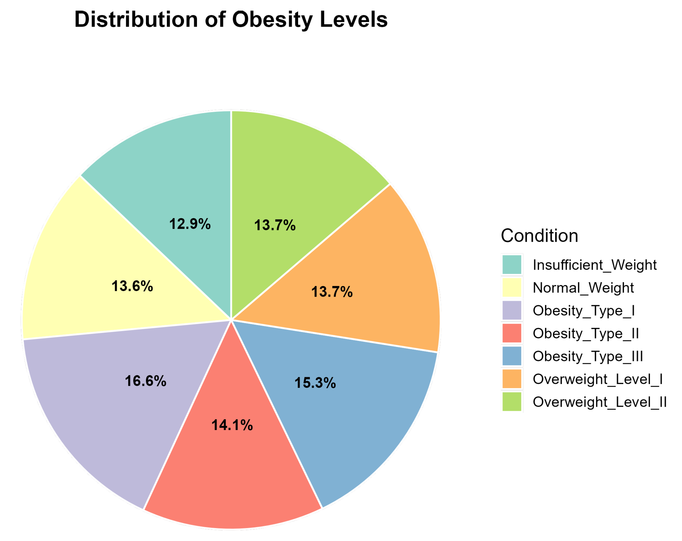
Figure 2.
Top 15 predictors of obesity classification ranked by mean decrease in Gini impurity across the 10 cross-validation folds (Random Forest). Weight (560.8) and Height (166.7) are the dominant features, followed by Age (150.3) and vegetable consumption frequency FCVC (142.7).
Figure 2.
Top 15 predictors of obesity classification ranked by mean decrease in Gini impurity across the 10 cross-validation folds (Random Forest). Weight (560.8) and Height (166.7) are the dominant features, followed by Age (150.3) and vegetable consumption frequency FCVC (142.7).
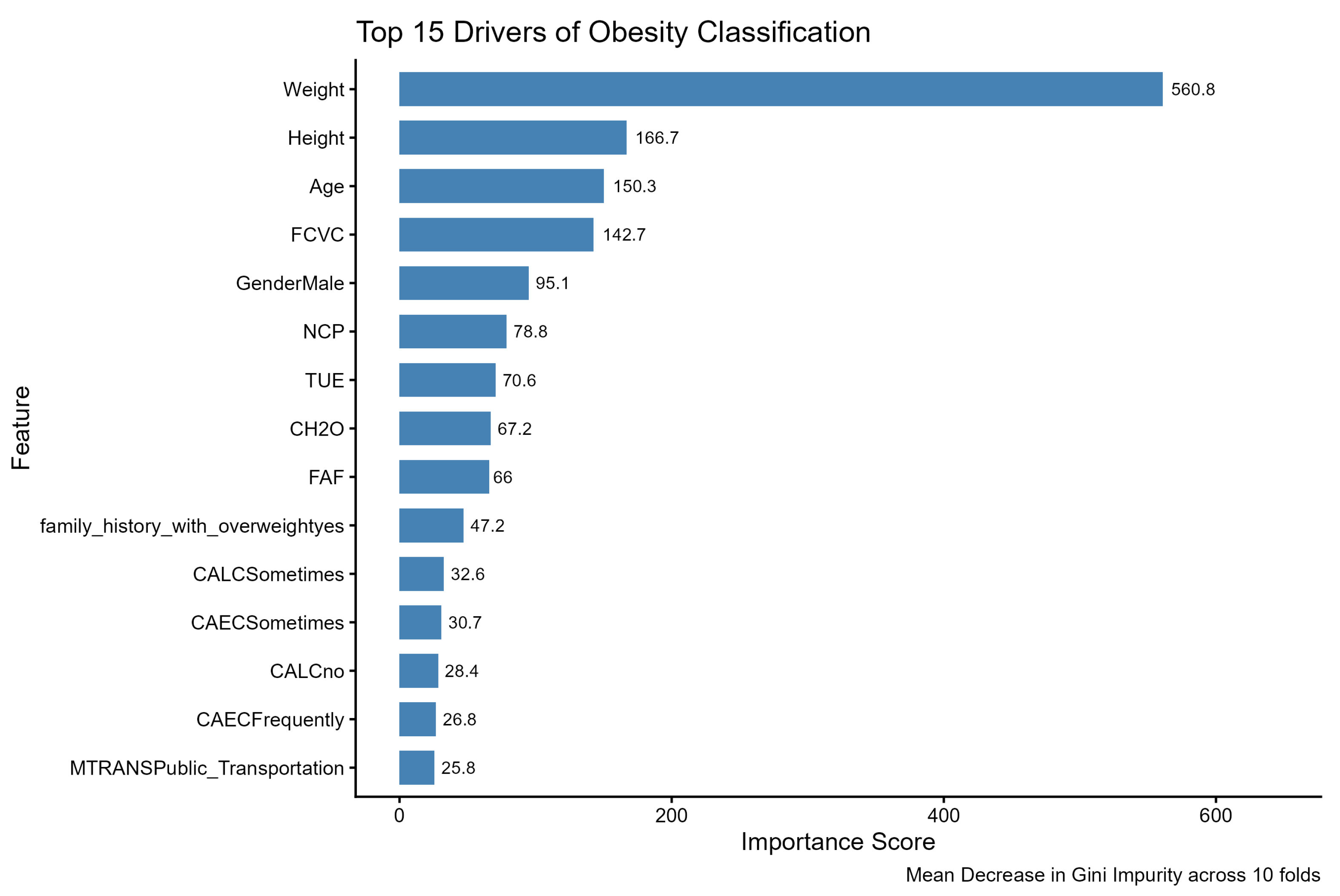
Figure 3.
PCA biplot of the standardized feature matrix, with 95% normal-theory confidence ellipses overlaid for each obesity class. The first principal component (PC 1) explains 19.0% of the total variance and the second (PC 2) explains 12.7%, together accounting for 31.7% of cumulative explained variance. The two components reveal largely distinct clustering across obesity categories, with the clearest separation between Insufficient Weight and higher obesity types.
Figure 3.
PCA biplot of the standardized feature matrix, with 95% normal-theory confidence ellipses overlaid for each obesity class. The first principal component (PC 1) explains 19.0% of the total variance and the second (PC 2) explains 12.7%, together accounting for 31.7% of cumulative explained variance. The two components reveal largely distinct clustering across obesity categories, with the clearest separation between Insufficient Weight and higher obesity types.
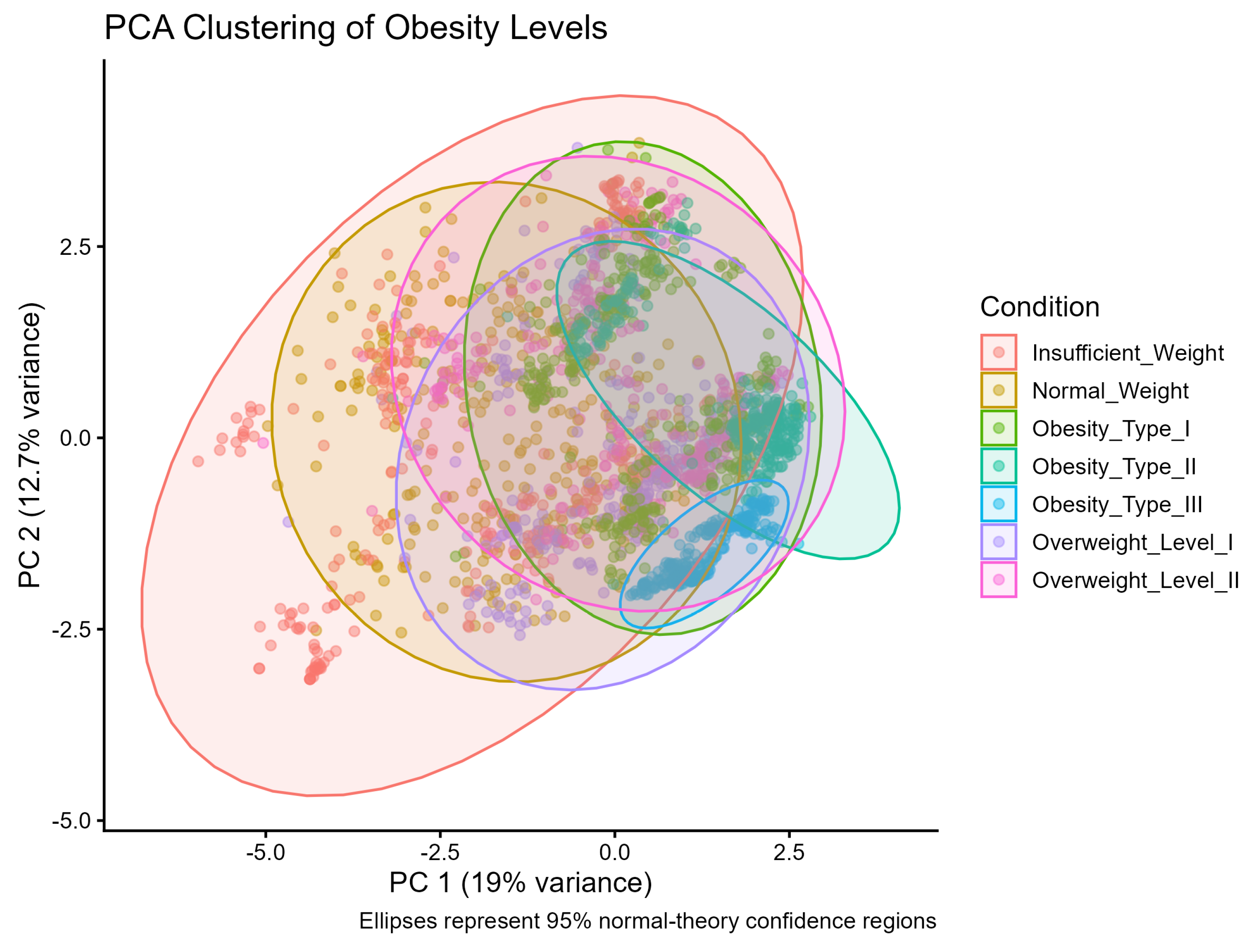
Figure 4.
Per-fold accuracy heatmap across the 10 cross-validation folds for all five models. XGBoost (rightmost column) is consistently the highest performer, with fold-level accuracy ranging from 95% to 99%, demonstrating stable generalization across all partitions.
Figure 4.
Per-fold accuracy heatmap across the 10 cross-validation folds for all five models. XGBoost (rightmost column) is consistently the highest performer, with fold-level accuracy ranging from 95% to 99%, demonstrating stable generalization across all partitions.
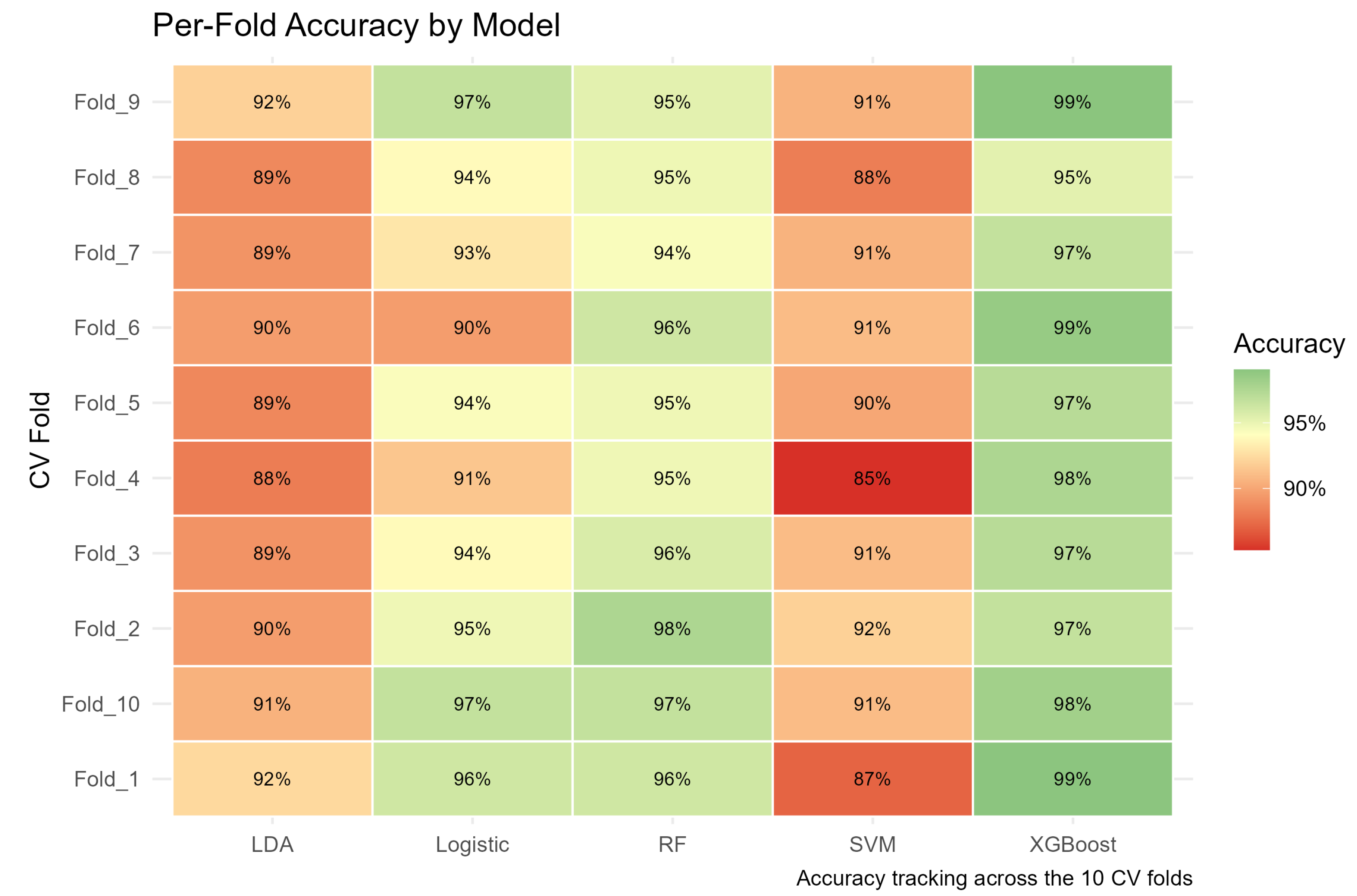

Table 1.
Descriptive Statistics of Key Physical Attributes by Gender.
| Female (n = 1,043) | Male (n = 1,068) | |||||
|---|---|---|---|---|---|---|
| Variable | Mean | SD | Range | Mean | SD | Range |
| Age (years) | 24.00 | 6.41 | 15.0–61.0 | 24.62 | 6.27 | 14.0–56.0 |
| Height (m) | 1.64 | 0.07 | 1.45–1.84 | 1.76 | 0.07 | 1.56–1.98 |
| Weight (kg) | 82.30 | 29.72 | 39.0–165.1 | 90.77 | 21.41 | 45.0–173.0 |
| Vegetables (FCVC) | 2.57 | 0.55 | 1.0–3.0 | 2.27 | 0.48 | 1.0–3.0 |
Table 2.
Model Performance Comparison (Macro-Averaged Metrics - 10-Fold CV).
| Model | Accuracy | Precision | Recall | F1 Score |
|---|---|---|---|---|
| XGBoost | 0.9754 | 0.9747 | 0.9748 | 0.9747 |
| Random Forest | 0.9564 | 0.9573 | 0.9551 | 0.9555 |
| Multinomial Logistic | 0.9403 | 0.9390 | 0.9388 | 0.9382 |
| Linear Discriminant Analysis | 0.8977 | 0.8969 | 0.8955 | 0.8935 |
| Support Vector Machine | 0.8967 | 0.8956 | 0.8939 | 0.8944 |
Table 3.
Confusion Matrix - XGBoost (10-Fold CV).
| Predicted ∖ Actual | Insuff. | Normal | Obesity I | Obesity II | Obesity III | Overwt I | Overwt II |
|---|---|---|---|---|---|---|---|
| Insufficient Weight | 267 | 6 | 0 | 0 | 0 | 0 | 0 |
| Normal Weight | 5 | 272 | 0 | 0 | 0 | 9 | 0 |
| Obesity Type I | 0 | 0 | 344 | 2 | 0 | 0 | 4 |
| Obesity Type II | 0 | 0 | 2 | 295 | 1 | 0 | 0 |
| Obesity Type III | 0 | 0 | 0 | 0 | 323 | 0 | 0 |
| Overweight Level I | 0 | 9 | 1 | 0 | 0 | 276 | 4 |
| Overweight Level II | 0 | 0 | 4 | 0 | 0 | 5 | 282 |
Table 4.
McNemar Pairwise Significance Tests (XGBoost vs. Alternative Models). All comparisons are statistically significant at .
Table 4.
McNemar Pairwise Significance Tests (XGBoost vs. Alternative Models). All comparisons are statistically significant at .
| Best Model | Alternative Model | p-value |
|---|---|---|
| XGBoost | Random Forest | (*) |
| XGBoost | Multinomial Logistic | (*) |
| XGBoost | Linear Discriminant Analysis | (*) |
| XGBoost | Support Vector Machine | (*) |
(*) Statistically significant at .
Disclaimer/Publisher’s Note: The statements, opinions and data contained in all publications are solely those of the individual author(s) and contributor(s) and not of MDPI and/or the editor(s). MDPI and/or the editor(s) disclaim responsibility for any injury to people or property resulting from any ideas, methods, instructions or products referred to in the content. |
© 2026 by the authors. Licensee MDPI, Basel, Switzerland. This article is an open access article distributed under the terms and conditions of the Creative Commons Attribution (CC BY) license (http://creativecommons.org/licenses/by/4.0/).
Copyright: This open access article is published under a Creative Commons CC BY 4.0 license, which permit the free download, distribution, and reuse, provided that the author and preprint are cited in any reuse.


