Kinks in the Discrete Systems in the Next to Leading Order Approximation: Josephson Transmission Line and Non-Linear Klein-Gordon Chains

1. Introduction

Interesting and potentially important examples of nonlinear transmission lines are circuits containing Josephson junctions [1] (JJ) - Josephson transmission lines (JTL) [2,3,4,5]. The weak kinks propagating in JTL were considered previously in the leading order (continuum). approximation [6,7]. The small parameter in the perturbation theory turns out to be the ratio of the JTL period to the kink width. In this paper we consider the kinks in the JTL in the next to leading order (quasi-continuum) approximation [7,8].

It turns out that the problem of the kinks in JTL has many similarities with the problem of kinks in the non-linear Klein-Gordon chains. The perturbation theory parameter also turns out to be the ratio of the chain period to the kink width. So we simultaneously consider the kinks in the ${\varphi }^4$ and sine-Gordon chains in the next to leading order approximation.

2. The Discrete Josephson Transmission Line

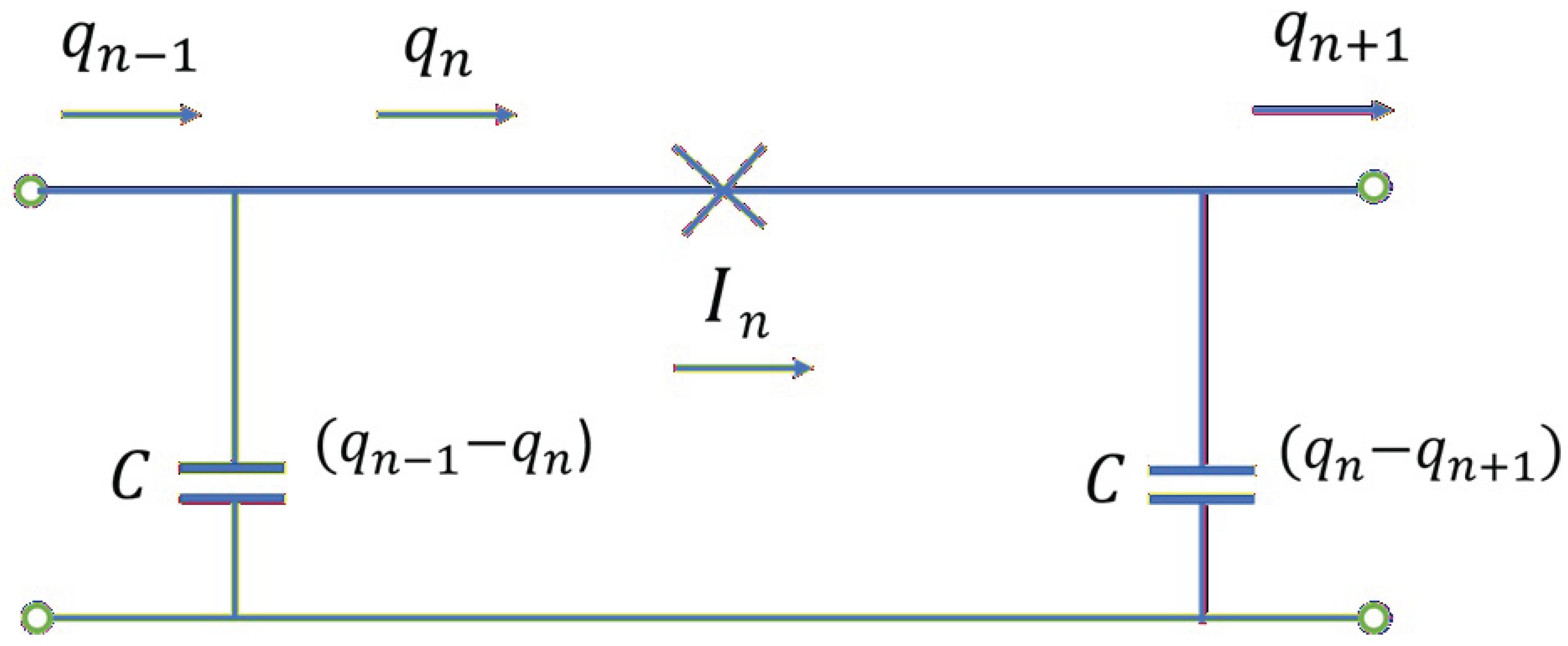
Consider the model of JTL constructed from identical JJ and capacitors, which is shown on Figure 1.

We take as dynamical variables the currents $I_n$ through the JJ and the charges $q_n$ which have passed through the JJ. The circuit equations are

$$\begin{array}{cc}\hfill {\displaystyle \frac{\hslash }{2e}}{\displaystyle \frac{d{\phi }_n}{d\tau }}& ={\displaystyle \frac{1}{C}}\left(q_{n+1}-2q_n+q_{n-1}\right),\hfill \end{array}$$

(1a)

$$\begin{array}{cc}\hfill {\displaystyle \frac{d{q}_n}{d\tau }}& =I_n,\hfill \end{array}$$

(1b)

where C is the capacitance.

Let us measure time in units of $\sqrt{L_{J}C}$, where $L_J=\hslash /\left(2e{I}_c\right)$, current through the JJ in units of the critical current of the JJ$I_c$, and charge in units of $I_c\sqrt{L_{J}C}$. Note that in this communication we read the Josephson law from right to left and consider the phase across the JJ as the function of the current [6,7,8,9]

$$\begin{array}{c}\hfill \phi ={sin}^{-1}I.\end{array}$$

(2)

The dimensionless form of Eq. (1) is

$$\begin{array}{cc}\hfill {\displaystyle \frac{d{\phi }_n}{d\tau }}& =D_2\left(q_n\right),\hfill \end{array}$$

(3a)

$$\begin{array}{cc}\hfill {\displaystyle \frac{d{q}_n}{d\tau }}& =I_n,\hfill \end{array}$$

(3b)

where $D_2$ is the discrete second derivative

$$\begin{array}{c}\hfill D_2\left(q_n\right)\equiv q_{n+1}-2q_n+q_{n-1}.\end{array}$$

(4)

To go from the difference to differential equations we introduce instead of the index n a continuous variables z and approximate the discrete second derivative by the infinite Taylor series

$$\begin{array}{c}\hfill D_2^{qc}={\displaystyle \frac{{\partial }^2}{\partial z^2}}+{\displaystyle \frac{1}{12}}{\displaystyle \frac{{\partial }^4}{\partial z^4}}+{\displaystyle \frac{1}{360}}{\displaystyle \frac{{\partial }^6}{\partial z^6}}+\dots \end{array}$$

(5)

(we measure z in the units of the transmission line period $\Lambda$). In the result Eq. (3) becomes

$$\begin{array}{cc}\hfill {\displaystyle \frac{\partial \phi }{\partial \tau }}& =D_2^{qc}\left(q\right)\hfill \end{array}$$

(6a)

$$\begin{array}{cc}\hfill {\displaystyle \frac{\partial q}{\partial \tau }}& =I\hfill \end{array}$$

(6b)

Note that Eq. (3) can be presented as

$$\begin{array}{c}\hfill {\displaystyle \frac{d^2{sin}^{-1}{I}_n}{d{\tau }^2}}=D_2\left(I_n\right),\end{array}$$

(7)

hence the speed of small and long wavelength oscillations on the constant background ${\phi }_1$ is given by the equation [7]

$$\begin{array}{c}\hfill u^2\left({\phi }_1\right)=cos{\phi }_1.\end{array}$$

(8)

We will see later that the expansion in (5) in our case is with respect to the powers of the kink amplitude, which we will consider as small. The forth order derivative in the r.h.s. of (5) is necessary to introduce the dispersion of the waves, thus allowing the existence of the kinks. Taking into account also the sixth order derivative gives the approximation we are after in this communication. Taking this term into account has additional advantage - the resulting Eq. (6) becomes non-singular at small wavelengths [7,8]. We’ll ignore all the higher order derivatives.

We are interested in the travelling wave solutions of the form

$$\begin{array}{c}\hfill I(z,\tau )=I\left(x\right),q(z,\tau )=q\left(x\right),\end{array}$$

(9)

where $x=U\tau -z$, and U is the wave speed. For these waves, partial derivative with respect to z in (5) becomes the ordinary derivative with respect to x, and Eq. (6) can be reduced to the ordinary differential equation for the current

$$\begin{array}{c}\hfill U^2{\displaystyle \frac{d\phi }{dx}}={\displaystyle \frac{dI}{dx}}+{\displaystyle \frac{1}{12}}{\displaystyle \frac{d^{3}I}{d{x}^3}}+{\displaystyle \frac{1}{360}}{\displaystyle \frac{d^{5}I}{d{x}^5}}.\end{array}$$

(10)

Integrating (10) with respect to x we obtain

$$\begin{array}{c}\hfill {\displaystyle \frac{1}{12}}{\displaystyle \frac{d^{2}I}{d{x}^2}}+{\displaystyle \frac{1}{360}}{\displaystyle \frac{d^{4}I}{d{x}^4}}=U^2\phi -I+F,\end{array}$$

(11)

where F is the constant of integration. Multiplying both sides by $dI/dx$ we may integrate (11) to obtain

$$\begin{array}{c}\hfill {\displaystyle \frac{1}{2}}{\left({\displaystyle \frac{dI}{dx}}\right)}^2+{\displaystyle \frac{1}{30}}\left[{\displaystyle \frac{dI}{dx}}{\displaystyle \frac{d^{3}I}{d{x}^3}}-{\displaystyle \frac{1}{2}}{\left({\displaystyle \frac{d^{2}I}{d{x}^2}}\right)}^2\right]=\Pi \left(I\right),\end{array}$$

(12)

where

$$\begin{array}{c}\hfill \Pi \left(I\right)=12\int \left(U^2{sin}^{-1}I-I+F\right)dI\end{array}$$

(13)

We are interested in the waves defined by the boundary conditions

$$\begin{array}{c}\hfill \underset{x\to -\infty }{lim}I\left(x\right)=I_2,\underset{x\to +\infty }{lim}I\left(x\right)=I_1.\end{array}$$

(14)

From Eq. (12) follows [7,8] that there exist two types of solutions: the kinks for which $I_2=-I_1$ and the solitons for which $I_2=I_1$. In both cases $\Pi \left(I\right)$ should be understood as $\Pi \left(I\right)-\Pi \left(I_1\right)$.

2.1. Weak Kinks

For the kinks the constants entering into (12) are

$$\begin{array}{cc}\hfill F& =0\hfill \end{array}$$

(15a)

$$\begin{array}{cc}\hfill U^2& ={\displaystyle \frac{I_1}{{sin}^{-1}{I}_1}},\hfill \end{array}$$

(15b)

hence (13) takes the form

$$\begin{array}{c}\hfill \Pi \left(I\right)={\displaystyle \frac{12I_1}{{sin}^{-1}{I}_1}}{\int }_{I_1}^I\left({\displaystyle \frac{{sin}^{-1}I}{I}}-{\displaystyle \frac{{sin}^{-1}{I}_1}{I_1}}\right)IdI.\end{array}$$

(16)

We’ll consider $I_1$ as a small parameter. Looking at Eqs. (11) and (16) we realize that the forth derivative carries additional multiplier $I_1^2$ with respect to the second one. Now we understand why we were able to ignore the eighth and the higher order derivatives in the Taylor expansion in the r.h.s. of (5) – they give the corrections beyond the order we are looking for.

In the leading order we can discard the second term in the l.h.s. of (12) and keep in (16) only the first two terms in the Taylor expansion of ${sin}^{-1}I/I$

$$\begin{array}{c}\hfill {\displaystyle \frac{{sin}^{-1}I}{I}}=1+{\displaystyle \frac{1}{2}}{\displaystyle \frac{I^2}{3}}+{\displaystyle \frac{1·3}{2·4}}{\displaystyle \frac{I^4}{5}}+\dots .\end{array}$$

(17)

Thus we can present Eq. (12) in the leading order as

$$\begin{array}{c}\hfill {\left({\displaystyle \frac{dI}{dx}}\right)}^2={\left(I^2-I_1^2\right)}^2.\end{array}$$

(18)

In the next to leading order approximation we should keep additionally the third term in the expansion of ${sin}^{-1}(I/I)$ in (16). After simple algebra we obtain

$$\begin{array}{c}\hfill \Pi \left(I\right)={\displaystyle \frac{1}{2}}\left(1+{\displaystyle \frac{3}{10}}{I}^2+{\displaystyle \frac{13}{30}}{I}_1^2\right){\left(I^2-I_1^2\right)}^2.\end{array}$$

(19)

In this approximation we also should take into account the second term in the l.h.s. of (12), but we can substitute into it the leading order solution of (18), which satisfies the relation

$$\begin{array}{c}\hfill {\displaystyle \frac{dI}{dx}}={\displaystyle \frac{I_1^2}{{cosh}^{2}y}},y\equiv I_{1}x;\end{array}$$

(20)

hence we can use the approximation (A3). So we obtain Eq. (12) in the next to leading order approximation

$$\begin{array}{c}\hfill \left[1+{\displaystyle \frac{2}{15}}{I}_1^2\left(2{tanh}^{2}y-1\right)\right]I_1^2{\left({\displaystyle \frac{dI}{dy}}\right)}^2\\ \hfill =\left\{1+{\displaystyle \frac{1}{30}}{I}_1^2\left[9{tanh}^{2}y+13\right]\right\}{\left(I^2-I_1^2\right)}^2.\end{array}$$

(21)

The solution of (21) with the accepted precision is

$$\begin{array}{c}\hfill I\left(x\right)=I_{1}tanh\tilde{y},\end{array}$$

(22)

where

$$\begin{array}{ccc}\hfill \tilde{y}& =& \int \left[1+{\displaystyle \frac{1}{60}}{I}_1^2\left({tanh}^{2}y+17\right)\right]dy\hfill \\ & =& \left(1+{\displaystyle \frac{3}{10}}{I}_1^2\right)y-{\displaystyle \frac{1}{60}}{I}_1^{2}tanhy.\hfill \end{array}$$

(23)

2.2. Weak Solitons

Though the paper studies kinks in the next to leading order approximation, just for fun let us present here study of weak solitons in the leading order approximation. By weak we’ll mean the solitons for which $I\approx I_1$. We’ll expand $\Pi \left(I\right)$ given by Eq. (13) with respect to the powers of $I-I_1$ and truncate the series after the third term, thus obtaining

$$\begin{array}{c}\hfill \Pi \left(I\right)=12{\int }_{I_1}^I\left\{U^2{sin}^{-1}{I}_1-I_1+F\right.\\ \hfill \left.+{\displaystyle \frac{\beta }{3}}\left(I-I_1\right)+{\displaystyle \frac{\gamma }{2}}{\left(I-I_1\right)}^2\right\}dI,\end{array}$$

(24)

where

$$\begin{array}{cc}\hfill \beta & =3\left({\displaystyle \frac{U^2}{cos{\phi }_1}}-1\right)\hfill \end{array}$$

(25a)

$$\begin{array}{cc}\hfill \gamma & ={\displaystyle \frac{U^2{I}_1}{{cos}^3{\phi }_1}}.\hfill \end{array}$$

(25b)

From the boundary conditions (14) follows that the term with the zero power of $\left(I-I_1\right)$ in the integrand in (24) should be equal to zero (which defines the integration constant F). Calculating the integral we obtain Eq. (12) in the leading approximation

$$\begin{array}{c}\hfill {\displaystyle \frac{1}{2}}{\left({\displaystyle \frac{dI}{dx}}\right)}^2=2\beta {\left(I-I_1\right)}^2+2\gamma {\left(I-I_1\right)}^3.\end{array}$$

(26)

Now we understand that the expansion parameter in series (24) is the difference between $U^2$ and $u^2\left({\phi }_1\right)=cos{\phi }_1$ (see Eq. (8)), which we here assume to be small (and positive). The solution of (26) is dark soliton

$$\begin{array}{c}\hfill I=I_1-{\displaystyle \frac{\beta }{\gamma {cosh}^2\sqrt{\beta }x}}.\end{array}$$

(27)

3. Kinks in Non-Linear Klein-Gordon Chains

Let us apply the method presented above to non-linear Klein-Gordon chains, described by the equation

$$\begin{array}{c}\hfill {\displaystyle \frac{d^2{\varphi }_n}{d{\tau }^2}}=D_2\left({\varphi }_n\right)+h^{2}F\left({\varphi }_n\right),\end{array}$$

(28)

where $F\left(\varphi \right)$ is some non-linear function and h (proportional to the chain period) will be treated as a small parameter. We again go from the discrete equation to a continuous one. This time in the next to leading order approximation it is enough to take into account only the first two terms in the series (5). Thus we obtain

$$\begin{array}{c}\hfill {\displaystyle \frac{{\partial }^2\varphi }{\partial {\tau }^2}}={\displaystyle \frac{{\partial }^2\varphi }{\partial z^2}}+{\displaystyle \frac{1}{12}}{\displaystyle \frac{{\partial }^4\varphi }{\partial z^4}}+h^{2}F\left(\varphi \right),\end{array}$$

(29)

where we’ll consider h as small parameter. We are interested in the travelling wave solutions of the form

$$\begin{array}{c}\hfill \varphi (z,\tau )=\varphi \left(x\right),\end{array}$$

(30)

where $x=U\tau -z$, and U is the wave speed. Thus we obtain the ordinary differential equation

$$\begin{array}{c}\hfill {\displaystyle \frac{d^2\varphi }{d{v}^2}}+{\alpha }^2{\displaystyle \frac{d^4\varphi }{d{v}^4}}=-F\left(\varphi \right).\end{array}$$

(31)

where

$$\begin{array}{cc}\hfill {\alpha }^2& \equiv {\displaystyle \frac{h^2}{12(1-U^2)}}\hfill \end{array}$$

(32a)

$$\begin{array}{cc}\hfill v& \equiv {\displaystyle \frac{hx}{\sqrt{1-U^2}}}.\hfill \end{array}$$

(32b)

Multiplying both sides of (31) by $d\varphi /dv$ we may integrate the equation to obtain

$$\begin{array}{c}\hfill {\displaystyle \frac{1}{2}}{\left({\displaystyle \frac{d\varphi }{dv}}\right)}^2+{\alpha }^2\left[{\displaystyle \frac{d\varphi }{dv}}{\displaystyle \frac{d^3\varphi }{d{v}^3}}-{\displaystyle \frac{1}{2}}{\left({\displaystyle \frac{d^2\varphi }{d{v}^2}}\right)}^2\right]=\Pi \left(\varphi \right),\end{array}$$

(33)

where

$$\begin{array}{c}\hfill \Pi \left(\varphi \right)=-\int F\left(\varphi \right)d\varphi .\end{array}$$

(34)

In the leading order with respect to $\alpha$ Eq. (33) takes the form

$$\begin{array}{c}\hfill {\displaystyle \frac{1}{2}}{\left({\displaystyle \frac{d\varphi }{dv}}\right)}^2=\Pi \left(\varphi \right).\end{array}$$

(35)

In the next to leading order we should take into account the second term in the l.h.s. of Eq. (33), but we can substitute into it the solution of (35).

We will be interested in the kinks defined by the boundary conditions

$$\begin{array}{c}\hfill \underset{x\to -\infty }{lim}\varphi \left(x\right)={\varphi }_2,\underset{x\to +\infty }{lim}\varphi \left(x\right)={\varphi }_1.\end{array}$$

(36)

where ${\varphi }_1$ and ${\varphi }_2$ are two zeros of $F\left(\varphi \right)$

$$\begin{array}{c}\hfill F\left({\varphi }_1\right)=F\left({\varphi }_2\right)=0,\end{array}$$

(37)

Below we consider the kinks in two important particular cases of the chains.

3.1. ${\varphi }^4$ Chain

For the ${\varphi }^4$ chain [10]

$$\begin{array}{c}\hfill F\left(\varphi \right)=\varphi \left(1-{\varphi }^2\right).\end{array}$$

(38)

Hence

$$\begin{array}{c}\hfill \Pi \left(\varphi \right)={\displaystyle \frac{1}{2}}{\left(1-{\varphi }^2\right)}^2\end{array}$$

(39)

and for the solution of (35) we obtain

$$\begin{array}{c}\hfill {\displaystyle \frac{d\varphi }{dv}}={\displaystyle \frac{1}{{cosh}^{2}v}}\end{array}$$

(40)

(we have chosen ${\varphi }_1=-{\varphi }_2=1$). Using (A3) and (A4) we obtain Eq. (33) in the next to leading order approximation as

$$\begin{array}{c}\hfill {\left({\displaystyle \frac{d\varphi }{d\tilde{v}}}\right)}^2={\left(1-{\varphi }^2\right)}^2,\end{array}$$

(41)

where

$$\begin{array}{c}\hfill \tilde{v}=\left(1-2{\alpha }^2\right)v+4{\alpha }^{2}tanhv.\end{array}$$

(42)

The solution of (41) is

$$\begin{array}{c}\hfill \varphi \left(x\right)=tanh\tilde{v}.\end{array}$$

(43)

3.2. Sine-Gordon Chain

For the sine-Gordon chain [11]

$$\begin{array}{c}\hfill F\left(\varphi \right)=-sin\varphi .\end{array}$$

(44)

Hence

$$\begin{array}{c}\hfill \Pi \left(\varphi \right)=1-cos\varphi \end{array}$$

(45)

and for the solution of (35) we obtain

$$\begin{array}{c}\hfill {\displaystyle \frac{d\varphi }{dv}}={\displaystyle \frac{2}{coshv}}\end{array}$$

(46)

(we have chosen ${\varphi }_2=0$, ${\varphi }_1=2\pi$). Using (A3) and (A4) we obtain Eq. (33) in the next to leading order approximation as

$$\begin{array}{c}\hfill {\left({\displaystyle \frac{d\varphi }{d\overline{v}}}\right)}^2=4{sin}^2(\varphi /2),\end{array}$$

(47)

where

$$\begin{array}{c}\hfill \overline{v}=\left(1-{\displaystyle \frac{{\alpha }^2}{2}}\right)v+{\displaystyle \frac{3{\alpha }^2}{2}}tanhv.\end{array}$$

(48)

The solution of (47) is

$$\begin{array}{c}\hfill \varphi =4{tan}^{-1}\left(exp\overline{v}\right),\end{array}$$

(49)

4. Discussion

We have calculated the kinks in several non-linear discrete equations in the next to the leading order approximation. The well known results for the kinks in the leading order approximation are obtained by putting $\tilde{y}=y$ in Eq. (22), $\tilde{v}=v$ in Eq. (43) and $\overline{v}=v$ in Eq. (49).

For the Klein-Gordon chains the perturbation theory expansion parameter was the ratio of the chain period to the kink width. For the JTL the perturbation theory expansion parameter formally was the kink amplitude. However, looking at Eq. (20) we realize that the expansion parameter in Section 2.1 is identical to that in Section 3.

Note that that for the discrete JTL, the leading order approximation corresponds to keeping the first two terms in series (5). The next to leading order approximation corresponds to taking into account the first three terms in the series (the quasi-continuum approximation). For the non-linear Kine-Gordon chains, continuum approximation corresponds to keeping only the first term in series (5). The next to leading order approximation corresponds to taking into account the first two terms.

In al the cases we considered, the next to leading order approximation changes the shape of the kink calculated previously in the leading order approximation. The change depends upon the ratio of the chain period to the kink width. From Eq. (23) follows that the higher order terms compress the kink in the discrete JTL. From Eqs. (42) and (48) follows that the higher order terms compress the central part of the kinks in the considered Klein-Gordon chains but make their wings broader.

References

- Josephson, B. D. Possible new effects in superconductive tunneling. Phys. Rev. Lett. 1962, 1, 251. [Google Scholar] [CrossRef]
- Barone, A.; Paterno, G. Physics and Applications of the Josephson Effect; John Wiley & Sons, Inc, New York, 1982. [Google Scholar]
- Pedersen, N. F. Solitons in Josephson Transmission lines, in Solitons; North-Holland Physics Publishing: Amsterda, 1986. [Google Scholar]
- Giovanella, C.; Tinkham, M. Macroscopic Quantum Phenomena and Coherence in Superconducting Networks; World Scientific: Frascati, 1995. [Google Scholar]
- Kadin, A. M. Introduction to Superconducting Circuits; Wiley and Sons: New York, 1999. [Google Scholar]
- Katayama, H.; Hatakenaka, N.; Fujii, T. Analogue Hawking radiation from black hole solitons in quantum Josephson transmission lines. Phys. Rev. D. 2020, 102, 086018. [Google Scholar] [CrossRef]
- Kogan, E. The kinks, the solitons and the shocks in series connected discrete Josephson transmission lines. Phys. Stat. Sol. (b) 2022, 259, 2200160. [Google Scholar] [CrossRef]
- Kogan, E. Josephson transmission line revisited. Phys. Stat. Sol. (b) 2023, 260, 2200475. [Google Scholar]
- Mohebbi, H. R.; Majedi, A. H. Shock Wave Generation and Cut off Condition in Nonlinear Series Connected Discrete Josephson Transmission Line. IEEE Trans. Appl. Supercond. 2009, 19, 891. [Google Scholar] [CrossRef]
- Roy, I.; Dmitriev, S.V.; Kevrekidis, P.G.; Saxena, A. Comparative study of different discretizations of the ϕ4 model. Phys. Rev. E 2007, 76, 026601. [Google Scholar]
- Peyrard, M.; Kruskal, M. D. Kink dynamics in the highly discrete sine-gordon system. Phys. 14D 1984, 88. [Google Scholar]
Disclaimer/Publisher’s Note: The statements, opinions and data contained in all publications are solely those of the individual author(s) and contributor(s) and not of MDPI and/or the editor(s). MDPI and/or the editor(s) disclaim responsibility for any injury to people or property resulting from any ideas, methods, instructions or products referred to in the content. |
© 2026 by the authors. Licensee MDPI, Basel, Switzerland. This article is an open access article distributed under the terms and conditions of the Creative Commons Attribution (CC BY) license (http://creativecommons.org/licenses/by/4.0/).
Copyright: This open access article is published under a Creative Commons CC BY 4.0 license, which permit the free download, distribution, and reuse, provided that the author and preprint are cited in any reuse.