

Submitted:
15 June 2026
Posted:
29 June 2026
You are already at the latest version
Abstract
A novel axiomatic foundation of entropy has recently been proposed overcoming the limitations of classical and information-theoretic entropy foundations and eventually unifying probabilistic and physical entropy. A new set of postulates leads to a rigorous, uncertainty-based definition of entropy consistent with the principle of maximum entropy. Entropy is thus a purely stochastic concept quantifying uncertainty, thereby completing Kolmogorov’s probability system. Applied to gas thermodynamics, the new framework reproduces classical results and derives, rather than assumes, the laws of thermodynamics. In atmospheric applications, entropy maximization yields an isothermal state as the molecular equilibrium. Gravitation does not alter the isothermal state but distinguishes it from the isentropic one of macroscopic air parcels, whose motion drives the atmosphere away from equilibrium. Radiatively active gases, through interactions with shortwave and longwave radiation, sustain non-equilibrium vertical profiles of the atmospheric variables. Combined with the Stefan-Boltzmann law, these mechanisms provide a simple, parsimonious and coherent explanation of observed atmospheric behaviours and the climatic system. The framework highlights thermodynamics as emergent from stochastics, offering new insights into molecular uncertainty, emergence of macroscopic structures and radiation in shaping Earth’s climate. It also suggests a broader stochastic view of nature and atmospheric processes.
Keywords:
stochastic thermodynamics
; maximum entropy
; atmospheric equilibrium
; gravitation
; radiative cooling
«Πολλὰ ἀπιστία δέδρακεν ἀγαθὰ ‹καὶ› πίστις κακά. ὅ τε Ἐπίχαρμος "μέμνασο ἀπιστεῖν" φησίν· "ἄρθρα ταῦτα τῶν φρενῶν." αὐτίκα τὸ μὲν ἀπιστεῖν τῇ ἀληθείᾳ θάνατον φέρει ὡς τὸ πιστεύειν ζωήν, ἔμπαλιν δὲ τὸ πιστεύειν τῷ ψεύδει, ἀπιστεῖν δὲ τῇ ἀληθείᾳ εἰς ἀπώλειαν ὑποσύρει.» ("Incredulity has brought about many good things, and trust evil things. And Epicharmus says, ‘Don't forget to exercise incredulity; for it is the sinews of the mind.’ Now, just as believing in the truth brings life, so does disbelieving in it bring death; but on the other hand, believing in lies, while disbelieving in the truth, leads to ruin. Clement of Alexandria [1]
1. Introduction
The basic premise of this work, which has been presented in detail in recent books by Koutsoyiannis (2025 [2], 2026 [3]), is that entropy is uncertainty quantified and is associated with change. As further clarified elsewhere [4,5], uncertainty is not ambiguity, confusion, fuzziness, disorder or a “monster”. Rather, uncertainty (or randomness, which is the same) is a fundamental governing principle of nature. Uncertainty makes the world interesting, life liveable, and humanity capable of freedom.
However, uncertainty needs to be described with clarity and accuracy—or, in Aristotle’s language, with saphenia [2,3]. The language to this aim is offered by stochastics—a collective name for probability theory, statistics and stochastic processes. Uncertainty and its quantified version, entropy, are not just a modelling convenience; they are the actual physics driving the reality we observe.
This reality is continuously changing, while the very notion of time would be meaningless without change. The nature of change has been a central philosophical issue from ancient times, as testified by quotations such as:
Deterministic laws are essentially conservation laws (for mass, momentum, energy, etc.). Conservation does not cause change. There should be a quantity that is not conserved—and this is entropy. This is the driving force of change as it tends to take its maximum allowed value. This tendency is mathematically expressed by the principle of maximum entropy for which the following formulation is proposed:
Uncertainty will not be lower than its maximum possible value without a reason.
Such a reason, if it exists, would be expressed mathematically as a constraint, as we will see below. It is stressed that, as is typical of first principles, the principle of maximum entropy, with its above formulation, is posited axiomatically and not derived or proved. Hence, its validity is not subject to proof, but is confirmed (or refuted) by the richness, reliability and consistency of the results it yields. Furthermore, contrary to the usual epistemological interpretation, the principle is here advanced as an ontological—hence physical—principle.
Even the colloquial meaning of the name entropy is related to change; it is etymologized from the Greek word εντροπία, a synthesis of εν (= in) and τροπή (= change; cf. troposphere). As a scientific term, entropy was introduced by Rudolf Clausius in 1865 [8], who understood the connection of entropy with change and its tendency to increase until it reaches a maximum. However, his classical thermodynamic definition is circular. He defined entropy, , for a reversible processes by , where is heat and temperature, and where a reversible process is one in which this equality holds—otherwise . Furthermore, he did not connect entropy with probability or uncertainty.
Ludwig Boltzmann (1872 [9], 1877 [10]) gave entropy its probabilistic content as he linked it to probabilities of thermodynamical system states. He thus explained the Second Law of thermodynamics as the tendency of a system to run toward more probable states, which have higher entropy. Boltzmann was followed by Gibbs (1902 [11]) and Planck (1906-1914 [12,13]), who regarded entropy as a probabilistic concept but without formal mathematical completeness. Note that Kolmogorov’s probability system had not been proposed at the time. It is interesting that Planck arrived at the same entropic formula in thermodynamics as the one that later Shannon (1948 [14]) did for information content. Shannon also called the quantity he arrived at entropy at von Neumann’s suggestion. According to his definition, entropy is a probabilistic concept, a measure (as Shannon incorrectly calls it) of information or, equivalently, of uncertainty.
Wiener (1948 [15]) also used the same definition for information, albeit with the opposite sign. Von Neumann (1956 [16]) obtained virtually the same definition of entropy as Shannon, though in a slightly different way. As von Neumann was a mathematician, physicist, computer scientist and engineer, he clearly understood the connection of the information-based entropy definition with its pre-existing physical content. He cited Szilard (1929 [17]), who had implied the same definition of entropy in a thermodynamic system. (Perhaps he was not aware of the earlier contributions by Planck).
Jaynes (1957 [18]) introduced the principle of maximum entropy, albeit not as a physical (ontological) principle, but one for logical inference (epistemological), with a formulation different from that given above. Specifically, his formulations was:
“in making inferences on the basis of partial information we must use that probability distribution which has maximum entropy subject to whatever is known.”
Interestingly, Jaynes (2003 [19]) insisted that probabilistic and thermodynamic entropies are different.
Given the above substantial contributions of famous scientists, one would expect that the existing foundation of entropy is fully satisfactory. However, it may be argued that it is not. Specifically, Shannon [14] derived the entropy formula by positing three “properties”, which are mathematically problematic—particularly the last one based on an example, rather than a mathematically rigorous statement [2]. Khinchin (1957) tried to give a proper mathematical foundation to Shannon’s theory using a different variant of Shannon’s postulates and demonstrating a “Uniqueness Theorem”, but he used the notion of conditional entropy before defining entropy [2].
Jaynes [19] (p. 347) reformulated Shannon’s postulates in a more general wording, which however did not satisfy even himself, as he noted:
Although the above demonstration appears satisfactory mathematically, it is not yet in completely satisfactory form conceptually. The functional equation (11.7) [the problematic Shannon’s example reformulated by Jaynes] does not seem quite so intuitively compelling as our previous ones did. In this case, the trouble is probably that we have not yet learned how to verbalize the argument leading to (11.7) in a fully convincing manner. Perhaps this will inspire others to try their hand at improving the verbiage that we used just before writing (11.7).
Papoulis (1991 [20], p. 533) claimed that he used Shannon’s postulates, whom he cited, after rephrasing them in a better mathematical language, but what he wrote was inaccurate (as demonstrated by counterexamples by Koutsoyiannis, [2]).
The above limitations and shortcomings give room to introduce a new foundation serving the need for mathematical rigor, consistency with maximum entropy as an ontological principle, and seamless connection to stochastic processes. In this new foundation, rather than follow Jaynes suggestion for “improving the verbiage” it was preferred to abandon these problematic postulates altogether and replace them with more satisfactory ones.
Hopefully this is done below in section 2. Applied to gas thermodynamics, the new framework reproduces classical results and derives, rather than assumes, the laws of thermodynamics in general and their application in the atmosphere simply by entropy maximization (section 3). Radiation laws, namely the Planck’s Radiation Law and the Stefan-Boltzmann Law, are also produced by entropy maximization (section 4) thus completing the simple, parsimonious and coherent explanation of observed atmospheric behaviours and the climatic system. Overall the framework (further discussed in section 5 and summarized in section 6) highlights thermodynamics as emergent from stochastics, offering new insights into molecular uncertainty, emergence of macroscopic structures and radiation in shaping Earth’s climate. It also suggests a broader stochastic view of nature and atmospheric processes.
Due to the wide range of the topics covered, on the one hand, and the requirement for brevity, on the other hand, the full set of derivations and their proofs is not contained in the paper, but can be found in [3], which serves as supplementary material for the paper.
2. Proposed Stochastic Foundation of Entropy
2.1. Preliminaries: Partitions, Probability, and Uncertainty
Probability, as defined by Kolmogorov (1933), is a normalized measure. Practically speaking, (excluding non-measurable sets), probability is a function that assigns numbers to events, where events are represented as sets. Events are subsets of a ground set, , whose elements are called outcomes. Any subset of which includes any number of outcomes is also an event. The ground set is also an event, the certain event, and has probability 1. All other events are uncertain. In typical problems there is an infinite number of outcomes (possibilities) and an even greater number of events. Given two events we can tell which is more uncertain by comparing their probability.
Entropy is a quantification of a set of events, which are disjoint and their union is the entire ground set. This set of events is called a partition. While probability assigns one number to each event, entropy assigns a single number to the entire set of events (partition or distribution). In this respect, it is not a measure. Figure 1 provides a schematic that helps intuition about the concepts involved.
It is useful to list here a few of the fundamental properties of partitions:
- The coarsest partition has one element,
- The finest partition is composed of elementary events, .
- A partition with two elements, is called a bipartition.
- A refinement of a partition is a partition such that each element of is a subset of some element of .
- A common refinement of two partitions is a refinement of both.
- Given two ground sets and partitions thereof , their product partition, denoted as , is a partition of the cartesian product , consisting of all events for all . Since the occurrence of the event is equivalent to the occurrence of both and , we can simplify the notation by omitting ‘’ and writing .
2.2 Postulates and the Derivation of the Entropic Formula
We need to define the entropic function (the green layer in Figure 1 ) in such a way that it incorporates the principle of maximum entropy. Namely, we should specify states associated with maximum uncertainty and make our definition such as to give a function that becomes maximum at these states. The following postulates assure this.
Postulate 1, Continuity
: Given a partition
of the ground set
, its entropy is a twice continuously differentiable function of the probabilities of the events that form the partition. Namely, , i.e.,.
This is a general postulate, specifying the form of entropy as a function of probabilities.
Postulate 2,Zero at certainty: The entropy of the coarsest partition is zero,
This is an obvious postulate, saying that a certain event has zero uncertainty.
Postulate 3, Non-interaction: There is no interaction between any two elements of a partition:
.
This is posited for consistency with the principle of maximum entropy: Had this second derivative been nonzero, the knowledge of would provide some information on and therefore would decrease uncertainty—without a reason.
Postulate 4, Maximization at independence: If are two identical ground sets, and are partitions thereof, then the entropy of the product partition is maximized when any paired events are independent, i.e., .
This is also posited for consistency with the principle of maximum entropy: Independence between two events results in maximum uncertainty as the occurrence of does not contain any information about the occurrence of .
Based on the four postulates we specify the form of, completing the entropy definition, through the following two theorems:
Theorem 1: There exists a univariate function such that
Theorem 2: The function in equation (1) is uniquely determined as
where
is a constant.
Based on these, we derive the entropic formula (also depicted in Figure 1) as
and we readily observe that, as is a dimensionless quantity, so will also be the entropy . The following corollaries, whose proofs are direct, express useful properties of entropy:
Corollary 1: Entropy is determined by equation (3) uniquely up to a constant multiplier.
Corollary 2: (with when or ).
Corollary 3: is a concave function of .
Corollary 4: For independent , the entropy of the product partition is
Corollary 5: For any ground sets and partitions thereof
with equality holding when are independent.
Corollary 4 is called the additivity property (or additivity principle) and verbally expressed as “the total entropy of two or more independent systems is equal to the sum of their individual entropies”. According to corollary 5, that sum is the maximum that a product partition can reach. Additional theorems and corollaries that give important properties of entropy can be found in [3].
Entropy can also be expressed in terms of expectations of functions of stochastic variables, considering the finest partition. Specifically, it is readily seen that for a discrete stochastic variable taking integer values (where could be infinite) with the entropy (of the finest partition) is:
For a continuous stochastic variable taking real values ) the definition of the entropy of is possible by means of the relative entropy. This is defined in terms of a background measure , either normalized (so that ) or not. If not, the most typical (but not exclusive) case for continuous variables is the Lebesgue measure, which for an interval (or ) equals the length . For any background measure, the relative entropy is defined as:
It is noted that other names (e.g. Kullback–Leibler divergence or cross-entropy) have also been in use for the same concept. To define the entropy of a continuous stochastic variable, first we take the finest partition for intervals of size , form the relative entropy for measure , and make the partition with elements ,
where is the distribution function. Then we take the limit of and set , so that . Hence:
It is important to note that for discrete variables entropy is a nonnegative number (any number between 0 and ∞) but for continuous variables the (relative) entropy can take any real value (between –∞ and ∞).
The importance of entropy stems from the very fact that it quantifies uncertainty in a rigorous manner. The associated principle of maximum entropy formally expresses the fact that uncertainty rules in nature. By maximizing entropy we determine the distribution of uncertain quantities, formally expressed as stochastic variables. This determination is made in a precise manner and within an inference framework that is deductive (αποδεικτικό/ apodeictic according to Aristotle), i.e. the strongest possible. Maximization is a very strong mathematical operation, which can determine any number of unknown quantities. In typical problems we have to determine an infinite number of unknowns, such as the probabilities of an infinite number of possibilities, but a single maximization suffices to determine them all. With entropy maximization we do not get the exact values of the variables involved (this would eliminate uncertainty and contradict the very principle of maximum entropy) but the probabilities thereof.
3. Applications to Atmospheric Thermodynamics
3.1. Premises
To find the state of the atmosphere we maximize entropy at the lowest level: the uncertainty of molecules in motion. For each molecule the uncertainty comprises several components:
- Location: Three location coordinates,
- Velocity: Three coordinates, , each bearing kinetic energy proportional to ; the number of degrees of freedom is thus .
- Angular momentum (transformed into velocity units, expressing additional, i.e. rotational, degrees of freedom): (a) for monoatomic molecules (e.g., Ar): no angular momentum and hence no additional degrees of freedom (); (b) for diatomic molecules (e.g., N₂, O₂) and triatomic molecules with linear structure (e.g., CO₂): two rotational degrees of freedom, corresponding to two axes of rotation (); (c) for triatomic molecules with nonlinear structure (e.g., H₂O) or polyatomic molecules: three additional degrees of freedom, corresponding to three axes of rotation ().
Following the principle of maximum entropy, the uncertainty is maximum at the microscopic (molecular) level. Because of the large number of molecules (of the order of the Avogadro’s number, , representing the number of particles per mole of substance) the uncertainty is practically eliminated at the macroscopic level (. This should not mislead us to think that thermodynamic laws are deterministic.
3.2 Entropy of Gas Molecules
First we consider a monatomic molecule of mass , moving rapidly in a motionless cube with edge (volume )[21], whose exact position and velocity are unknown. Its state is described by 6 variables, 3 indicating its position and 3 indicating its velocity with all represented as stochastic variables, forming the vector . The constraints for the particle’s position are . We use a non-relativistic framework and therefore we do not constrain velocity. The feasible space, , is thus (0, a) for each and () for each ().
The conservation of energy demands that: where is the energy per particle (known as internal or thermal energy) and . Hence, the energy constraint is .
We form the entropy of as in equation (9), recognizing that the background density in should have units [z–1] = [x–3] [u–3] = [L–6 T3]. To form this, we utilize a universal constant, i.e., the Planck constant = 6.626 × 10⁻³⁴ J·s, whose dimensions are [L2 M T–1]. If we combine it with a reference mass (such as the particle’s or the proton’s mass), we observe that the quantity has the required dimensions [L–6 T3], thereby giving the entropy as
Application of the principle of maximum entropy with constraints for conservation of mass (i.e., total probability equal to 1), momentum and energy gives the distribution of as:
as it is shown that it satisfies all constraints. This is the multivariate normal distribution for velocity and the uniform for location.
Combining equations (10) and (11), and performing the integration over we find the final expression of entropy:
where e is the base of natural logarithms and are constants with units of energy and volume, respectively, satisfying
so that the middle term of the equation equals the rightmost one. Note that one of is a freely chosen parameter. Equation (12) reflects the fact that the entropy is a dimensionless quantity, as it should according to its definition in section 2, and its rightmost part is the sum of two dimensionless quantities representing energy and space available to motion.
An extended version of equation (12) (for many particles; see below), but with some differences (see section 3.3), is known as the Sackur-Tetrode equation (after Sackur [22] and Tetrode [23], who developed it independently at about the same time in early 1910s).
Generalizing for a molecule with degrees of freedom moving in the same cube we again find a multivariate normal distribution for velocity and uniform for location, i.e.:
where , is the energy associated with the ith degree of freedom with being equal to the mass for and related to the rotational inertia for the other coordinates, and is the geometric mean of , i.e., .
The maximized entropy of the molecule is
where is a physical constant incorporating the Planck’s constant, the proton mass and a reference moment of inertia, and are constants appropriately chosen to match the rightmost with the middle term.
If, instead of 1, we have identical molecules moving in the same cube of volume , and with average energy per molecule , each with degrees of freedom, then the unknown quantity is the vector with 3N location coordinates and βN motion coordinates. With mass, momentum and energy constraints expressed in terms of expectations of the related stochastic variables, the entropy maximizing distribution is found to be the product of the distribution functions of the individual molecules:
This clearly suggests: (a) independence of the motion of different molecules, (b) uniform distribution for their location and (c) multivariate normal distribution for their velocity. The entropy for N molecules is the sum of the entropies of the individual molecules (additivity property):
3.3 Standardized (Intensive and Extensive) Entropies
The entropies determined above for one or molecules do not precisely correspond to those in standard use in physics, because they are not intensive and extensive respectively. To restore full correspondence, we take the entropies conditional on a partition 𝔹, in which only the molecule location, discretized into bins, matters. The entropy of this partition for 1 and molecules are, respectively and .
We denote the total energy and the total volume, with being the average volume per molecule. The non-standardized (original) and standardized (conditional on ) entropies for 1 molecule are, respectively:
The non-standardized (original) and standardized (conditional on ) entropies for molecules are respectively:
The standardized entropies and are intensive and extensive, respectively, while the original ones, and do not have these properties. However, the descriptions by either the original or the standardized entropies are precisely equivalent, once the probability calculus for each case is correct. The original quantities are more effective, and hence preferable, in explaining behaviours regarded as paradoxical (e.g., the Gibbs paradox [24]).
3.4 Definition of Temperature and Relation to Classical Thermodynamics.
In classical thermodynamics, temperature is regarded as a foundational concept. In our stochastic framework, the foundational concepts are the energy and the entropy , with the temperature being a derivative:
In a gas with molecules in motion with average energy per particle degrees of freedom, the temperature is obtained as:
Here the temperature has energy units and differs from the classical temperature in physics, , measured in kelvins. The unit of kelvin was an arbitrary choice (a historical accident) which in our framework is rendered an energy unit: 1 K = 13.80649 yJ. Yet the two quantifications are equivalent: The temperature in our framework is proportional to the classical temperature , as is the entropy in our framework with respect to the classical entropy . The proportionality relationships are given through Boltzmann’s constant = 1.38 × 10⁻²³ J K−1:
3.5 Ideal Gas Law
To find the pressure, p, at the box shown in Figure 2 we calculate which molecules hit the base of the cube at a time interval and with which velocity. Namely, the molecules in question are those satisfying .
Knowing the distribution function of , we integrate and find the expectation of the momentum of those molecules. Using Newton’s Second Law, we calculate the expectation of the force exerted on the face, and dividing by the area we calculate the pressure. The result is (in natural units of temperature and for denoting the volume per molecule):
Converting to SI and using the universal gas constant or the specific gas constant , where is the molar mass, we find the classical form of the ideal gas law:
where n is the number of moles in the volume and is the density.
3.6 Specific Heats and Comparison with Observations
The specific heat in thermodynamics reflects just the degrees of freedom. For a gas with degrees of freedom and gas constant , the specific heat under constant volume (isochoric), , and under constant pressure (isobaric), , are:
Table 1 shows the gases appearing in Earth’s atmosphere in proportions > 0.05%, and their characteristics as derived by our stochastic framework. Experimental values for are also given and compared with theoretical values. The deviations are smaller than 1% except for the most complex case of water vapour, in which it is 2%.
3.7 Interactions of Bodies
Our framework of entropy maximization can infer by deduction the final states of systems brought into contact, without using the principles of thermodynamics, both in equilibrium cases, but also in non-equilibrium cases. We summarize the most interesting results here, the derivation of which can be found in [3].
In equilibrium cases we maximize the entropy under the typical constraints as above and assume that the entropy attains its maximum value allowed by the constraints after their interaction. Specifically:
- In a closed interaction, two systems A and B that are brought into contact, so that they can exchange energy but not mass, will have equal temperatures: .
- In an open interaction, in which the two systems can exchange both energy and mass, in the final state all intensive quantities will be equal: temperature, volume per particle, density, pressure and standardized entropy per particle. This expresses the macroscopic ultimate simplicity of a microscopically complex system.
- In an open interaction of two systems under gravitation, in which the one system is at an elevation higher than the other, the temperature in the two systems will be the same but all other intensive properties will differ.
For non-equilibrium cases, we just put an additional constraint expressing the reason why the systems are not allowed to reach equilibrium and we apply the same maximization framework. Specifically:
- In two systems in contact, a stable temperature difference could be sustained if there is a constant heat transfer. In this case, all quantities are determined from the temperature difference and there is no room for entropy maximization.
- In two systems far apart under gravitation, in which the one system is at an elevation higher than the other, a stable temperature difference can again be sustained if there is a constant heat transfer.
- In this case with isothermality excluded, entropy maximization results in an isentropic state: The standardized entropy per particle is the same in the two systems.
3.8 Equilibrium and Non-Equilibrium States of An Air Column
The state of an air column is generally affected by gravitation. However, gravitation does not alter the equilibrium state: It remains isothermal, the same as if gravitation were absent—a result verified by simulating molecule collisions under gravitation [25]. What gravitation does is to distinguish the isentropic state from the isothermal.
In reality, the Earth is not in equilibrium and hence the atmosphere is not isothermal. The non-equilibrium state is caused by changes occurring on all scales due to diverse mechanisms affecting radiation processes, both shortwave and longwave: day and night, cloud formation and disappearance, summer and winter, albedo’s spatial and temporal variation (also affected by biosphere changes), Sun’s dynamics and astronomical processes, orbital variations (Milanković cycles), tectonic and volcanic activity, and numerous other irregular changes by internal processes and external forces [26].
In absence of equilibrium, there is heat transfer. While in solids heat is transferred by conduction, in fluids (atmosphere and oceans) heat transfer is dominated by convection, i.e. mass flow. When mass flows, conduction can be neglected as its power is orders of magnitudes smaller than in convection. This is particularly the case for air, whose thermal conductivity is 25 times smaller than in water.
Therefore when there is convection, the macroscopic motion is mostly reversible adiabatic (where adiabatic means without heat exchange), i.e., isentropic. Ergo, the atmospheric temperature profile departs from the isothermal and tends to the isentropic.
3.9 Atmospheric Temperature Profiles
A specific solution of the differential equation of vertical heat transfer is a linear temperature profile,
with constant ) known as the lapse rate. The isothermal profile corresponds to constant temperature, exponential pressure decrease, and linear entropy increase:
On the other hand, the isentropic state is characterized by constant entropy and the following equations for dry air:
These two profiles are depicted in Figure 3, in comparison with four other, also having constant lapse rates: 6.5 K/km for the standard atmosphere (see section 3.11); –3 K/km for an inversion state, i.e., one with negative lapse rate; 12 K/km for a superadiabatic profile with steep gradient; and = 34.2 K/km for the so-called homogenous profile, in which the density is constant.
Real world profiles are not identical to any of the above theoretical ones, but change in time and space. However, all above lapse rate values (except the homogenous) do appear in reality (see examples in Figure 4), with the average lapse rate in the troposphere being close to ~6.5 K/km—that of the standard atmosphere.
The main reason for the standard lapse rate being smaller than the above calculated isentropic one of 9.8 K/km is that in that calculation the air was assumed dry. As explained in section 3.10, for air containing water vapour, the calculation is more complex and the resulting lapse rate smaller.
3.10 Phase Change, Saturation Vapor Pressure and Effect on the Isentropic Profile
To find the equilibrium state between the liquid and gaseous state of water, we maximize the uncertainty of single molecule with respect to: (a) its phase (whether gaseous or liquid); (b) its location in space; and (c) its kinetic state, i.e., its velocity and other coordinates corresponding to its degrees of freedom ( 6 in gaseous phase, 18 in liquid phase), all making up its thermal energy.
The final result for the saturation vapour pressure, , as a function of the temperature, , is:
where is an anchoring point (arbitrarily chosen) and is the amount of energy per molecule to break the bonds between molecules of the liquid phase in order for the molecule to switch to the gaseous phase (evaporation). If converted to SI units Equation (29) becomes:
where the point denotes the triple point of water. The agreement of the equation with measurements is excellent, better than in standard and empirical formulae [28,29]. Maximizing microscopic uncertainty we almost eliminated the macroscopic one, for the very reason discussed in section 3.1.
The equation determining the modified isentropic profile when water is present in the atmosphere in both gaseous (vapour) and liquid (clouds) phases is somewhat complicated and needs integration across the atmospheric column. The integration between any two states 0 and 1 gives the following relationship of the moist isentropic profile:
where is the latent heat of vaporization per molecule, and are the total pressure and saturation vapour pressure, respectively, and are the numbers of molecules of dry air and water, respectively, and is the number of water molecules that are in gaseous phase. Note that during the transition from state 0 to state 1, does not remain constant because of vapour condensation.
A simplified equation is obtained if we neglect the term . We call the resulting profile the wet isentropic profile, which approximates satisfactorily the pseudoadiabatic profile, in which the condensed water vapour precipitates immediately. In a lesser degree it also approximates the moist isentropic profile, in which the condensed water vapour remains in the atmosphere (clouds). Converted to SI units, the equation of the wet isentropic profile becomes:
In the latter equation, and are the temperature and pressure at any altitude , is the saturation vapour pressure, is the saturation mixing ratio (where and are the densities of water vapour and dry air, respectively), and is the latent heat of vaporization (in SI units). The subscripts ‘0’ and ‘D’ refer to the base level () and “dry air” case, respectively.
Figure 5 illustrates some instances of the wet isentropic profile, which depends on the surface temperature. For large temperatures, its slope is significantly smaller than in dry air.
For low surface temperature, the moist isentropic profile becomes practically indistinguishable from the dry isentropic profile because the low temperature does not allow much water to evaporate (or sublimate) to enter the gaseous phase. As a consequence, in polar regions the dry and wet isentropic profiles almost coincide with a lapse rate of 9.8 K/km. However, there, the actual rate is less than even that of the standard atmosphere of 6.5 K/km. Hence, the common argument that it is the moist isentropic state that fully determines the lapse rate in the troposphere is not accurate. Additionally, most of the time the atmosphere is not saturated and therefore the moist isentropic profile is not applicable. The climatic system is most complex, and both convection (vertical flow) and advection (through meridional winds) also play important roles. In particular, in the polar regions convection is weaker and thus the atmosphere remains closer to the isothermal profile than in tropical regions (see also section 3.11).
3.11 Standard Profiles of Earth’s Atmosphere
The standard atmosphere, i.e., a profile representative of year-round, midlatitude conditions (ICAO [30]), is depicted in Figure 6. It is seen that in the mesosphere, the temperature decreases with the increase of altitude as there is removal of heat from the atmosphere (cooling) due to emission of longwave radiation (see section 4). In the stratosphere, the pattern is opposite (inversion) because of the absorption of solar radiation, caused by the ozone layer reacting with the ultraviolet radiation. In the troposphere the temperature drops as the altitude increases, driven by convection (and not by radiation as many think).
Particular local profiles for different zones of the Earth (namely five different locality profiles) are compiled and used for MODTRAN (MODerate resolution atmospheric TRANsmission model), a code that performs detailed modelling of radiation in the atmosphere [31,32,33]. Three of these profiles are shown in Figure 7, along with data from ERA5 reanalysis (with ERA5 standing for the fifth generation atmospheric reanalysis of the European Centre for Medium-Range Weather Forecasts—ECMWF; ECMWF ReAnalysis [34]). These data are publicly available for the period 1940 onwards at a spatial resolution of 0.5°. Here they were retrieved from the WRIT [35] and ClimExp [36] platforms, with the former providing the entire data set and the latter that for the period 1950 onwards. The figure shows a good agreement of data with these profiles. The local profiles clearly reflect the connection with convection: In the polar regions and midlatitude winters, the atmosphere is closer to the isothermal profile than in tropics, because of the lower level of convection, whose full absence would necessarily lead to an isothermal atmosphere.
3.12 Cells or Air Parcels, and Macroscopic Motion
As shown in sections 3.1-3.9, if there were only molecular motion, the atmospheric profile would tend to the isothermal, driven by the principle of maximum entropy. However, there are macroscopic atmospheric structures, named cells or air parcels, which move as structures (convection), while being continually transformed in shape and physical characteristics.
These structures differ and expand in a hierarchy of spatiotemporal scales, starting with a spatial scale of mm to m and a temporal scale of min, and reaching the horizontal scale of a third of a hemisphere, the vertical scale of the entire troposphere, and the seasonal time scale. The hierarchy includes Rayleigh-Bénard cells, small thermals or plumes, mesoscale convection cells, deep convective cells, mesoscale convective systems, and global circulation cells. They are typically treated via continuum fluid dynamics, rather than molecular-level thermodynamics.
The coexistence of molecular and macroscopic motion at multiple scales determines the nonzero vertical temperature gradient. The macroscopic motion cannot retain constant temperature. Rather it drives the actual vertical temperature profile away from the isothermal. Indeed, an air parcel that has been warmed at the surface will move upward so fast that no heat can be removed from it, or added to it. Hence the process is reversible and adiabatic, i.e., isentropic. The lapse rate will then tend to the isentropic lapse rate, the dry one if the atmosphere is not saturated, or the wet one if it is saturated.
4. Extension to Radiation
4.1 Entropy of Radiation Quanta
In section 3 we treated the moving molecules by their kinetic energy, while we also investigated the effect of the potential energy due to gravitation. In steady state the energy and entropy remain unchanged. However, the kinetic energy of molecules tends to decay due to their emission of photons. Thus, in order for a system to remain in steady state it must receive energy equal to the emitted, and in order to be in equilibrium its entropy must be at maximum.
We assume that a molecule has average kinetic energy and within a certain time frame it emits an average energy as electromagnetic radiation (photons). It receives the same average amount of energy from the environment (e.g. by heat or radiation) and it remains at steady state. As radiation is a stochastic process, it has its own entropy , hence the total entropy of the molecule is
where is the entropy related to the kinetic state of the molecule. Here we have assumed additivity of entropy, which presupposes independence of the kinetic and the radiative processes—an assumption that in the problem examined is plausible, even though in other systems it is not (e.g. in strongly entangled quantum systems). Assuming a perturbation of radiative energy, in expense of the kinetic energy, so that , and taking derivatives with respect to we find:
From the definition of temperature, (equation (20)), we recognize that the last term, , is . The inverse of the term is the radiation temperature and since at equilibrium , from equation (34) we conclude that the radiation temperature is identical to the kinetic temperature, .
To determine the radiation entropy we recall that a photon is a quantum that cannot be subdivided and has minimal specific energy content, , where is the Planck constant and is the frequency. Integer multiples of the minimal energy are allowed and thus radiation materializes in quanta of energy , where is regarded as a realization of the stochastic variable with allowed values . Denoting , the entropy is:
The constraints are
After entropy maximization considering the constraints, the unknown probabilities are found to follow the geometric distribution, namely:
The average energy and entropy expressions, in terms of temperature, become, respectively:
Converting the average energy to power per unit area, we obtain Planck’s Law for blackbody radiation:
where is the spectral density expressed for frequency , is the spectral density expressed for wavelength , and denotes the speed of light in vacuum. The law determines the emitted radiation intensity. Converted to SI units, and are respectively expressed as W s m–2 sr–1 and W m–3 sr–1. Figure 8 illustrates the law for the spectrum of the solar (shortwave; SW) and terrestrial (longwave; LW) radiation.
4.2 Atmospheric Radiation Effect
The atmosphere is not transparent to radiation. As shown in Figure 9, several gases absorb and emit radiation at particular wavelengths. These are called radiatively active gases (RAGs) but are more commonly referred to by the misnomer “greenhouse gases” (see section 4.4). These include water vapour (condensing) and non-condensing gases (NC-RAG). The effect of RAGs and clouds on transmitted radiation is called atmospheric radiation effect (ARE) but is more commonly referred to by the misnomer “greenhouse effect”.
The ARE applies to both solar (SW) and terrestrial (LW) radiation. For the solar spectrum, the total power (area of spectrum) is 1361 and 735 W/m2 (reduction to 54%) at the top of the atmosphere and the surface, respectively. If reduced to Earth’s area (by division by 4), these become 340 and 184 W/m2, respectively.
4.3 The Stefan-Boltzmann Law and the Earth’s Equilibrium Temperature
The integral of the spectrum over the entire range of frequencies , is
Converting this to SI units and identifying it to emitted power per unit area, after integrating the radiant exitance over the outgoing hemisphere (units W/m2) we obtain:
where is the Stefan-Boltzmann constant. This is the Stefan-Boltzmann Law which applies to a blackbody, an idealized body with maximal emission. In a real object, typically called a grey body, the total radiation is lower by a factor , known as emissivity, i.e.:
The solar radiation, which is governed by the Stefan-Boltzmann Law at Τ = 5772 Κ, when reaching the Earth it is partly reflected and absorbed. Then the Earth emits at different wavelengths, determined by its own equilibrium temperature, where the meaning of equilibrium is that on the long term energy balance is achieved.
Therefore, it is not correct to say that the Sun feeds the Earth with energy. Rather, it is correct to say that the Sun feeds the Earth with low entropy, given that solar radiation is at higher frequencies than terrestrial and, entropy is a decreasing function of frequency. Indeed, from equation (38) we find:
Based on the Stefan-Boltzmann Law and using the trigonometric and astronomic details of Earth’s geometry and motion, we obtain the equilibrium temperature of Earth. The results are shown in Table 2 for the top of the atmosphere (TOA) and for the average albedo [3].
As seen in Table 2, the equilibrium temperature is not a uniquely defined magnitude, but, depending on several factors, it can range widely. For reasons explained in [3], the most realistic value is that on the bottom-right corner of in Table 2, or somewhat higher. We finally adopt the average temperature value of 255 K. A typical question is: Why is Earth’s surface temperature 288 K (estimated by averaging measurements at Earth’s surface), much higher than the equilibrium temperature (255 K)? The typical answer is: Because of the “greenhouse effect”. Here we examine another question: Is it higher (in a comparable way)?
In calculating the equilibrium temperature of 255 K we used the irradiance and albedo at the TOA, and thus we considered the Earth as a whole. On the other hand, at any location (defined by its geographical coordinates ) we do not have a unique Earth temperature across altitudes because the atmospheric column is not isothermal.
Since calculating the equilibrium temperature we considered the Earth as a whole, it is reasonable to assume that this value represents the average temperature over the atmospheric column. As seen in Figure 7, the column average temperature equals the actual one at an altitude of 5-7 km, which roughly corresponds to the atmospheric pressure level of 500 hPa.
As seen in Figure 10, based on ERA5 reanalysis data, the global average temperature at the level of 500 hPa is 258 K, close to 255 K, at an average altitude of 5.7 km. For a lapse rate of 6.5 K/km in the troposphere, a temperature of 255 K at this altitude yields a surface temperature of 292 K, close to 288 K.
4.4 Is the Atmosphere a Greenhouse?
A greenhouse is a structure designed to regulate the temperature and humidity of the environment inside. Such constructions had their origin in Roman times [38], and initially aimed to insulate a garden during the night. When greenhouses became common at the 17th century, they were outfitted with glass. In modern times the cover and walls can be plastic, usually low-density polyethylene (LDPE).
It was thought that the glass’s opacity to LW radiation was the mechanism causing warming of the greenhouse, by letting SW radiation in and trapping LW radiation. This is not accurate, as testified by both Roman and modern technology. In particular, LDPE is transparent to LW radiation.
In fact, in a real greenhouse, the mechanism of warming is the blocking of convection, which otherwise would transfer heat from the inside farther away. This is known since more than 100 years ago, by an experiment by Wood (1909) [39], who reported that “the loss of temperature of the ground by radiation is very small in comparison to the loss by convection; in other words […] we gain very little from the circumstance that the radiation is trapped”.
In contrast, in the atmosphere, warming occurs exactly through the process of convection. Without convection, the temperature profile would be isothermal (as is in a real greenhouse). An isothermal atmosphere would lead to a surface temperature of 255 K. Due to the opposite mechanisms, what has been called “greenhouse effect” for the atmosphere, should have better been called an “anti-greenhouse effect”.
As first highlighted by Aristotele, sapheneia (clarity and accuracy) of concepts and terminology is essential in science. The adoption of the wrong term “greenhouse effect” has several misleading consequences: mechanism mismatch (convection vs. radiation and implication of a static barrier); oversimplification and non-holistic view of complex processes; and unjustified emphasis on particular gases [25]. Here, as already mentioned, the terms radiatively active gas (RAG) and atmospheric radiative effect (ARE) are used.
4.5 How are the Vertical Temperature Gradient and ARE Linked?
This question cannot be answered merely from experimental evidence as it is difficult to control the lapse rate. It is also difficult to address it by deduction based on bulk entropy maximization, as we did in other questions. Therefore, to investigate the link of vertical temperature gradient and ARE, we use a radiation transmission model, namely RRTM (standing for rapid radiative transfer model), a hybrid physical/statistical approximation of the full line-by-line models, whose results have been extensively evaluated and validated [40]. The model implementation used here simulates the radiation flux through Earth’s atmosphere at a range of altitudes, calculating both SW (incoming and reflected sunlight) and LW (emitted by the ground and the atmosphere), both upward and downward. The model version used is an online application [41] and thus any interested reader can repeat the calculations and check the results.
Here RRTM was run with different lapse rates using default values for other parameters and assuming no clouds. (For runs with clouds present the interested reader is referred to [25].) The equilibrium temperatures obtained from the RRTM runs at the surface () and the TOA () are shown in Figure 11. For we get K (expected: ~255 K). For K/km we get K (reasonably below 288 K because of not considering clouds). Importantly, the surface temperature increases with for the same atmospheric composition and tends to become constant for high .
The most characteristic index for the behaviour of the atmosphere—with emphasis on the troposphere—is provided by the net radiative flux gradient , easily calculated from RRTM and depicted in Figure 12. To investigate the results shown in this graph, we use the following simplified form of the differential equation for the mono-dimensional heat transfer in fluids, written in SI units:
where and are the total vertical radiation and heat flux, respectively (in units of power per area). The equation holds for an atmosphere without conduction and convection, but can approximate an atmosphere with convection if the variables are regarded as temporal averages for time scales long enough, so that the expectation of the gradient could be assumed constant throughout (as observational data of the troposphere suggest) and hence .
We examine two special cases, where in the fist there is no vertical heat transfer, i.e.:
and in the second there is steady state, i.e.,
Furthermore we focus on the troposphere and denote the temperature at the surface and the tropopause, respectively, where the tropopause is assumed to be at the altitude of 11 km, as in the standard atmosphere. We compare these temperatures with that of an isothermal atmosphere, , which would be in between . We also denote the radiative heat flux gradient near the surface and the tropopause, respectively.
In the case of temperature inversion, we will have
From Figure 12, in both examined cases of inversion, –3 and –1 K/km, we have
If we assume no vertical heat transfer, then:
- near the surface we have, ; hence the layer will warm, and the temperature will tend to the isothermal, ;
- near the tropopause we have, ; hence the layer will cool, and the temperature will tend to the isothermal, .
That is, in both cases, an atmosphere with temperature inversion and no vertical heat transfer is unstable and its temperature profile will tend to the isothermal, which is stable according to molecular thermodynamics (sections 3.7 and 3.8). Similar tendency to the isothermal atmosphere applies to the superadiabatic case, K/km, but now because of the very positive and the negative in the upper atmospheric layers.
If we assume steady state for the cases of temperature inversion ( –3 and –1 K/km), then:
- near the surface, , which means that less energy leaves the layer from below than entering from above; since heat can only be absorbed by the layer, this means that the heat transfer is from upper layers downward;
- near the tropopause, , which means that more energy enters the layer from below than leaving it from above or we have upward transfer of energy.
That is, in steady state, heat should be created somewhere in between the surface and the tropopause and be transmitted both downward and upward, which seems absurd.
In the case of a regular atmospheric profile, i.e., cooling with increased altitude, we will have
From Figure 12, in the examined regular cases, K/km, we have
If we assume no vertical heat transfer, then across the entire atmosphere we have ; hence any layer will cool, which seems absurd. On the contrary, if we assume steady state, then across the entire atmosphere we have, , which means that more energy enters the layer from below than leaving it from above. Some energy is absorbed in the layer and we have upward transfer of energy. This is physically consistent, because . Actually, this suggests the development of convection to restore energy balance through .
For we have implying no heat transfer and no convection. Therefore, the isothermal state is stable both with and without RAGs. This conclusion stands in contrast to the classical claim by Manabe and Strickler (1964 [42]) who argued that, in absence of convection, a “pure radiative equilibrium” would produce a very steep lapse rate. According to their claim, this would lead to a surface temperature of 332.3 K due to the “greenhouse effect”.
Such claim is inconsistent with the RRTM results for surface temperature plotted in Figure 11. Moreover, the profile with the steepest gradient in Figure 12, 12 K/km, indicates that, without convection, we will have in the troposphere and in the stratosphere, i.e. a clear tendency to the isothermal profile. Therefore, the steep gradient cannot represent any form of stable “pure equilibrium” as Manabe and Strickler maintained. Furthermore, Manabe and Strickler’s results imply that convection would decrease the surface temperature while RRTM results and all other thermodynamic and radiative analyses presented in this work show the opposite. Hence Manabe and Strickler’s and RRTM results are inconsistent to each other.
One may counter than Manabe and Strickler’s “pure radiative equilibrium” is not associated with a linear vertical temperature profile. However, the asymptotically constant surface temperature for high lapse rates (clearly visible in Figure 11) and the general behaviour of the RRTM-derived radiative flux gradient (seen in Figure 12) make it paradoxical to suggest that a further increase in surface temperature, as suggested by Manabe and Strickler, would achieve radiative equilibrium without convection. On the contrary, all analyses converge on the conclusion that increasing the lapse rate enhances convection. A more detailed examination of this issue is not particularly meaningful, as it refers to idealized conditions irrelevant to reality, and therefore lies beyond the scope of this paper.
Coming back to the isothermal state (), we observe in Figure 12 a small negative in the lower atmospheric levels, which however is not deemed to be significant, as the accuracy of the model is not perfect. Also, an isothermal atmosphere would block convection and hence radically reduce evaporation. In RRTM the default value of humidity is 80%, and this was not modified in our model runs. If taken lower, the negative disappears. Hence, for the isothermal case (), RRTM confirms that the thermodynamic equilibrium in the troposphere () is also a radiative equilibrium (The above theoretical findings are supported by experimental and field evidence. Among laboratory experiments related to LW radiation from gases, the most sophisticated and informative ones are those of Harde and Schnell [43,44] and Schnell and Harde [45,46]. Their measurements were also confirmed by radiative transfer calculations. Their results suggested that ARE depends on the lapse rate. They provided experimental evidence that ARE can also have a cooling effect, which they called “negative greenhouse effect”.
Measurements by satellites also support the fact that, in case of inversion, the behaviour of ARE is reversed. Figure 13 (reproduction with adaptation of part of Figure 9 in [47]) shows the vertical intensities at the TOA observed from a satellite and modelled with radiation transfer theory for the Mediterranean and Antarctica.
In both cases, the agreement between observations and the detailed radiation model the authors conducted is remarkable. However, when compared to Planck’s law, remarkable differences are seen. In the Mediterranean there is a regular vertical temperature profile, with positive lapse rate. In contrast, in Antarctica, atmospheric inversion is almost permanent between the surface and the atmospheric level of 600 hPa [25]. In the Mediterranean, as a result of the ARE, the radiation intensity at the TOA is lower than that leaving the ground, where the latter is given by the curve of Planck’s Law. This has a warming effect on the ground. However, in Antarctica, the ARE amplifies the LW radiation that leaves the ground. This is tantamount to a cooling effect at all altitudes, including at the surface. Hence it is the vertical temperature profile that determines whether the ARE has either a warming or a cooling effect.
5. Discussion
The entropic-stochastic framework has several advantages, such as the unifying character, simplicity, parsimony, better alignment with quantum uncertainty, and resolution of paradoxes like the Gibbs paradox. Its relevance for hydrometeorology and the new insights it provides can explain a diversity of processes, including convection, lapse rates, moisture effects, radiation, and non-equilibrium states.
Future work would point out strengths and limitations, as well as required adaptations of the framework in additional tasks, such as full stochastic processes, turbulence, and climate implications. As an example, the assumption of independence at molecular scale needs to be adapted in studying turbulent motion.
With reference to classical thermodynamics, it is remarkable that all analyses presented here fully avoided using its four principles. Rather the principles are either derived or replaced by the new stochastic framework. In summary:
Zeroth Law: if two systems are in thermal equilibrium with a third system, then they are in thermal equilibrium with each other.
We did not need this law. Rather, we derived it from maximization of entropy.
First Law: it is related to the conservation of energy, which in classical thermodynamics takes a particular form distinguishing internal energy and work.
We used the conservation of energy as a first principle, from which the particular form used in thermodynamics is readily derived.
Second Law: it states that in the process of reaching a thermodynamic equilibrium, the total entropy of a system increases, or at least does not decrease.
We replaced it with the principle of maximum entropy applied to thermodynamic systems.
Third Law: it states that the entropy of a system approaches zero as the temperature approaches absolute zero.
We did not need this law at all. A slightly different form of the law is derived in [3] in which as the entropy approaches zero, the energy is not zero but a super-tiny quantity, smaller than the quantum zero-point energy that is imposed by Heisenberg’s uncertainty principle. Thus, our stochastic framework is in better agreement with quantum physics than the classical version which implies that zero energy is in principle feasible.
Additionally, the new farmwork enables broader philosophical and scientific implications in terms of comprehending and treating uncertainty and change, which are principal properties of Nature.
6. Conclusions
- A novel foundation of entropy has been proposed, grounded in stochastic principles and four postulates that naturally incorporate the principle of maximum entropy as an ontological (physical) law of nature, rather than merely an epistemological tool.
- The resulting entropy expression, uniquely derived, coincides with the classical Planck-Shannon form but rests on firmer mathematical and conceptual grounds, free from the circularities and limitations of previous formulations.
- This framework unifies probability, uncertainty, and change: entropy is uncertainty quantified, and its maximization drives the irreversible evolution of natural systems.
- In hydrometeorology and atmospheric thermodynamics, the approach allows deductive derivation of key physical laws and relations (temperature, ideal gas law, specific heats, dry and moist isentropic profiles, Clausius-Clapeyron equation, Planck’s radiation law) directly from stochastic principles and conservation of energy.
- The stochastic view reveals the atmosphere as a system governed by coexisting molecular and macroscopic randomness across scales, explaining why its temperature profile tends toward (but is not strictly) isentropic rather than isothermal.
- Overall, stochastics emerges not as a modelling convenience but as the actual physics underlying natural processes. This consideration offers clarity (saphenia), predictive power, and deeper insight into the workings of a fundamentally uncertain world.
Uncertainty is not a bug. It is the governing principle that makes the Universe alive.
Supplementary Materials
While there are no formal Supplementary Materials, the book in Ref. [3] provides additional information.
Author Contributions
Not applicable.
Funding
This research received no external funding and was rather conducted out of scientific curiosity.
Data Availability Statement
No new data were created in this study. The datasets used were retrieved from the sources described in detail in the text.
Acknowledgments
I thank Vassilios Zoukos and George Tsakalias for their comments and suggestions about materials related to this paper. I also thank Alberto Montanari for inviting me to present a preview of the paper’s material at the University of Bologna. During the preparation of the manuscript, I chatted with Grok (created by xAI) for the purposes of checking texts and mathematical derivations, and summarizing the material for the Conclusions section. I have considered the chats’ outputs but take full responsibility for the content of this publication.
Conflicts of Interest
I declare no conflicts of interest.
Abbreviations
The following abbreviations are used in this manuscript:
| ARE | Atmospheric radiation effect |
| ClimExp | Climate Explorer |
| ERA5 | Fifth generation atmospheric reanalysis of the European Centre for Medium-Range Weather Forecasts |
| ICAO | International Civil Aviation Organization |
| LDPE | Low-density polyethylene |
| LW | Longwave |
| MODTRAN | MODerate resolution atmospheric TRANsmission model |
| RAG | Radiatively active gas |
| RRTM | Rapid radiative transfer model |
| SI | Système international d'unités (International System of Units) |
| SW | Shortwave |
| TOA | Top of the atmosphere |
| WRIT | Web-based Reanalysis Intercomparison Tool |
References
- Clement of Alexandria, The Stromata, 4.3.8. Available online: http://www.poesialatina.it/_ns/greek/testi/Clemens/Stromata04.html (accessed on 7 June 2026).
- Koutsoyiannis, D. Stochastics of Hydroclimatic Extremes - A Cool Look at Risk. Edition 5, ISBN: 978-618-85370-0-2, 420 pages, doi: 10.57713/kallipos-1; Kallipos Open Academic Editions: Athens, 2025; Available online: http://www.itia.ntua.gr/2000/ (accessed on 7 June 2026).
- Koutsoyiannis, D. Stochastics as Physics; Edition 0 (incomplete); National Technical University of Athens: Athens, Greece, 2026; Available online: https://www.itia.ntua.gr/2600/ (accessed on 7 June 2026).
- Koutsoyiannis, D. A random walk on water. Hydrol. Earth Syst. Sci. 2010, 14, 585–601. [Google Scholar] [CrossRef]
- Koutsoyiannis, D.; Sargentis, G.-F. Entropy and Wealth. Entropy 2021, 23, 1356. [Google Scholar] [CrossRef] [PubMed]
- Heraclitus, quoted in Plato’s Cratylus. 439d, p. 440c.
- Aristotle. Meteorologica I.14, 353a 16.
- Clausius, R. A contribution to the history of the mechanical theory of heat. Phil. Mag. 1872, 43, 106–115. [Google Scholar] [CrossRef]
- Boltzmann, L. Weitere Studien über das Wärmegleichgewicht unter Gasmolekülen. Sitzungsberichte Akad. Wiss. Vienna Part II reprinted in Boltzmann's Wissenschaftliche Abhandlungen, Vol. I, Leipzig, J.A. Barth. 1909, 66(1872), 275-370 316-402. [Google Scholar]
- Boltzmann, L. Über die Beziehung zwischen dem zweiten Hauptsatze der mechanischen Wärmetheorie und der Wahrscheinlichkeitsrechnung respektive den Sätzen über das Wärmegleichgewicht. Wien. Ber. 1877, 76, 373–435. [Google Scholar]
- Gibbs, J.W. Elementary Principles in Statistical MechanicsYale University Press, New Haven, Connecticut, 1902. (Reprinted by Dover, New York, 1960 . Available online: https://www.gutenberg.org/ebooks/50992 (accessed on 7 June 2026).
- Planck, M. Vorlesungen über die Theorie der Wärmestrahlung.J. A. Barth, Leipzig . 1906. Available online: https://archive.org/details/vorlesungenberd03plangoog (accessed on 7 June 2026).
- Planck, M. The Theory of Heat Radiation; Blakiston, Philadelphia, Pennsylvania, USA, 1914; Available online: https://www.gutenberg.org/ebooks/40030 (accessed on 7 June 2026).
- Shannon, C.E. A mathematical theory of communication. Bell Syst. Tech. J. 27(379)(1948), 623–656. [CrossRef]
- Wiener, N. Cybernetics or Control and Communication in the Animal and the Machine; MIT Press: Cambridge, Mass., USA, 1948; 212 pp. [Google Scholar]
- von Neumann, J. Probabilistic logics and the synthesis of reliable organisms from unreliable components. Autom. Stud. 1956, 43–98. [Google Scholar] [CrossRef]
- Szilard, L. Über die Entropieverminderung in einem thermodynamischen System bei Eingriffen intelligenter Wesen. Z. Für Phys. 1929, 53(11), 840–856. [Google Scholar]
- Jaynes, E.T. Information theory and statistical mechanics. Phys. Rev. 1957, 106(4), 620–630. [Google Scholar] [CrossRef]
- Jaynes, E.T. Probability Theory: The Logic of Science; Cambridge Univ. Press: Cambridge, UK, 2003; p. 728 pp. [Google Scholar]
- Papoulis, A. Probability, Random Variables and Stochastic Processes, 3rd edn; McGraw-Hill: New York, 1991. [Google Scholar]
- See a 2D animation at https://commons.wikimedia.org/wiki/File:Translational_motion.gif and a simulation in a gravitational field at https://www.itia.ntua.gr/2537/ (Supplementary material - Video in high or low resolution). both accessed on. (accessed on 7 June 2026).
- Sackur, O. Die Anwendung der kinetischen Theorie der Gase auf chemische Probleme. Ann. Der Phys. 1911, 36, 958–980. [Google Scholar] [CrossRef]
- Tetrode, H. Die chemische Konstante der Gase und das elementare Wirkungsquantum. Ann. Der Phys. 1912, 38, 434–442. [Google Scholar] [CrossRef]
- Koutsoyiannis, D. Physics of uncertainty, the Gibbs paradox and indistinguishable particles. Stud. Hist. Philos. Mod. Phys. 2013, 44, 480–489. [Google Scholar] [CrossRef]
- Wagner, W.; Pruss, A. The IAPWS formulation 1995 for the thermodynamic properties of ordinary water substance for general and scientific use. J. Phys. Chem. Data 2002, 31, 387–535. [Google Scholar] [CrossRef]
- Koutsoyiannis, D.; Tsakalias, G. Unsettling the settled: Simple musings on the complex climatic system. Front. Complex Syst. 2025, 3, 1617092. [Google Scholar] [CrossRef]
- University of Wyoming Atmospheric Science Radiosonde Archive. Available online: https://weather.uwyo.edu/upperair/sounding.shtml (accessed on 7 June 2026).
- Koutsoyiannis, D. Clausius-Clapeyron equation and saturation vapour pressure: simple theory reconciled with practice. Eur. J. Phys. 2012, 33(2), 295–305. [Google Scholar] [CrossRef]
- Koutsoyiannis, D. Entropy: from thermodynamics to hydrology. Entropy 2014, 16(3), 1287–1314. [Google Scholar] [CrossRef]
- Doc 7488/3ICAO (International Civil Aviation Organization) Manual of the ICAO Standard Atmosphere: Extended to 80 Kilometres / 262,500 Feet, 3rd Ed. ed; ICAO: Montreal, Canada, 1993; p. 304 pp.
- Berk, A.; Bernstein, L.S.; Robertson, D.C. MODTRAN: A Moderate Resolution Model for LOWTRAN; Air Force Geophysics Laboratory, Air Force Systems Command, United States Air Force: Hanscom Air Force Base, Massachusetts, USA, 1987; Available online: https://apps.dtic.mil/sti/pdfs/ADA185384.pdf (accessed on 7 June 2026).
- Berk, A.; Acharya, P.K.; Bernstein, L.S.; Anderson, G.P.; Lewis, P.; Chetwynd, J.H.; Hoke, M.L. Band model method for modeling atmospheric propagation at arbitrarily fine spectral resolution . U.S. Patent #7433806, 2008. [Google Scholar]
- Berk, A.; Conforti, P.; Kennett, R.; Perkins, T.; Hawes, F.; van den Bosch, J. MODTRAN6: A Major Upgrade of the MODTRAN Radiative Transfer Code . Proc. SPIE 2014, 9088, 90880H. [Google Scholar] [CrossRef]
- Hersbach, H.; Bell, B.; Berrisford, P.; Biavati, G.; Horányi, A.; Muñoz Sabater, J.; Nicolas, J.; Peubey, C.; Radu, R.; Rozum, I.; Schepers, D.; Simmons, A.; Soci, C.; Dee, D.; Thépaut, J.-N. ERA5 hourly data on single levels from 1940 to present. Copernic. Clim. Change Serv. (C3S) Climate Data Store (CDS) 2023. [Google Scholar] [CrossRef]
- WRIT (Web-based Reanalysis Intercomparison Tool) Monthly Timeseries, NOAA Physical Sciences Laboratory. Available online: https://psl.noaa.gov/data/atmoswrit/timeseries/ (accessed on 7 June 2026).
- ClimExp (Climate Explorer). Koninklijk Nederlands Meteorologisch Instituut (KNMI): de Bilt, The Netherlands, 2022; Available online: https://climexp.knmi.nl (accessed on 7 June 2026).
- Wikimedia Commons. Available online: https://commons.wikimedia.org/ (accessed on 7 June 2026).
- Janick, J.; Paris, H. History of controlled environment horticulture: Ancient origins. HortScience 2022, 57(2), 236–238. [Google Scholar] [CrossRef]
- Wood, R.W. Note on the theory of the greenhouse. Philos. Mag. Ser. 1909, 17(98), 319–320. [Google Scholar] [CrossRef]
- Mlawer, E.J.; Taubman, S.J.; Brown, P.D.; Iacono, M.J.; Clough, S.A. Radiative transfer for inhomogeneous atmospheres: RRTM, a validated correlated-k model for the longwave. J. Geophys. Res. Atmos. 1997, 102(D14), 16663–16682. [Google Scholar] [CrossRef]
- RRTM Earth's Energy Budget. Available online: https://climatemodels.uchicago.edu/rrtm/ (accessed on 7 June 2026).
- Manabe, S.; Strickler, R.F. Thermal equilibrium of the atmosphere with a convective adjustment. J. Atmos. Sci. 1964, 21(4), 361–385. [Google Scholar] [CrossRef]
- Harde, H.; Schnell, M. Verification of the greenhouse effect in the laboratory. Sci. Clim. Change 2022, 2(1), 1–33. [Google Scholar] [CrossRef] [PubMed]
- Harde, H.; Schnell, M. The negative greenhouse effect – part II, Studies of infrared gas emission with an advanced experimental set-up. Sci. Clim. Change 2025. [Google Scholar] [CrossRef] [PubMed]
- Schnell, M.; Harde, H. Model-experiment of the greenhouse effect. Sci. Clim. Change 2023, 3(5), 445–462. [Google Scholar] [CrossRef] [PubMed]
- Schnell, M.; Harde, H. The negative greenhouse effect – part I, Experimental studies with a common laboratory set-up. Sci. Clim. Change 2025. [Google Scholar] [CrossRef] [PubMed]
- van Wijngaarden, W.A.; Happer, W. Radiation transport in clouds. Sci. Clim. Change 2025, 5(1), 1–12. [Google Scholar] [CrossRef] [PubMed]
- Hanel, R.A.; Conrath, B.J. Thermal emission spectra of the Earth and atmosphere from the nimbus 4 Michelson interferometer experiment. Nature 1970, 228, 143–145. [Google Scholar] [CrossRef] [PubMed]
Figure 1.
Schematic for the basic concepts required for entropy definition: ground set, outcomes, events, partition, and probability and entropy as functions.
Figure 1.
Schematic for the basic concepts required for entropy definition: ground set, outcomes, events, partition, and probability and entropy as functions.
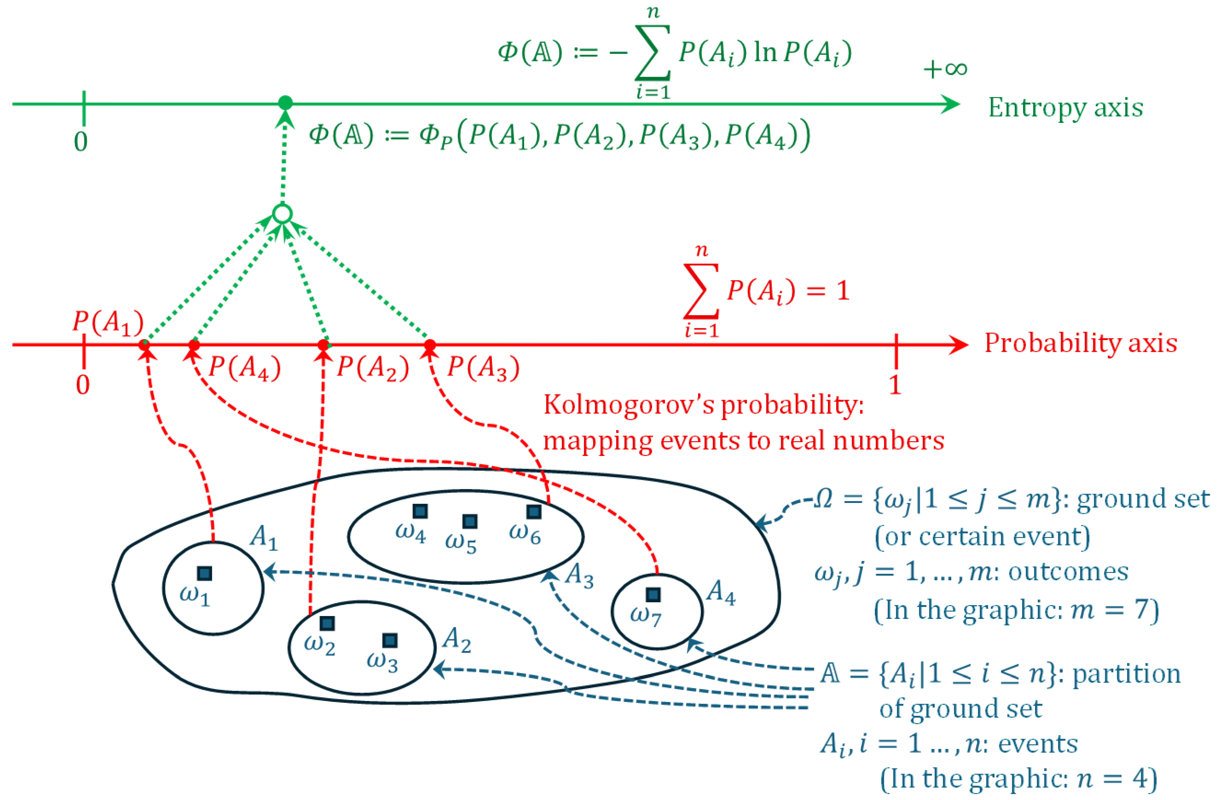
Figure 2.
Explanation sketch for the collision of a molecule to the bottom face of a cube. The particle shown, located at coordinate (distance from the bottom face), will collide with the bottom face () within time if . The other location and velocity coordinates do not play any role: for example, if and/or are large, a possible collision with the rightmost face of the cube will result in horizontal reflection that will not alter the velocity coordinate .
Figure 2.
Explanation sketch for the collision of a molecule to the bottom face of a cube. The particle shown, located at coordinate (distance from the bottom face), will collide with the bottom face () within time if . The other location and velocity coordinates do not play any role: for example, if and/or are large, a possible collision with the rightmost face of the cube will result in horizontal reflection that will not alter the velocity coordinate .
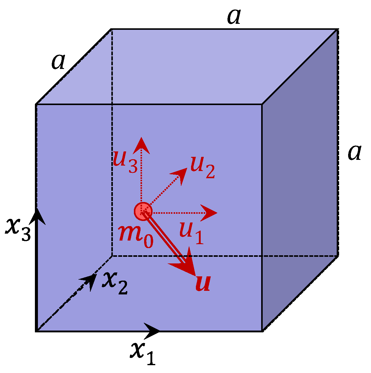
Figure 3.
(left) Temperature difference, (middle) pressure ratio and (right) difference of entropy per unit mass at elevation with respect to the values at zero elevation for the indicated states for dry air. The lapse rates are: 0 (isothermal ); 9.8 K/km (isentropic); = 34.2 K/km (homogenous); and 6.5 K/km (standard atmosphere). The specific rates chosen for illustration of the superadiabatic and inversion states are 12 K/km and –3 K/km, respectively. In the leftmost graph the temperature at zero elevation can be any value, while for the other graphs it is 288 K (continuous lines), 258 K (dotted lines) and 303 K (dashed lines).
Figure 3.
(left) Temperature difference, (middle) pressure ratio and (right) difference of entropy per unit mass at elevation with respect to the values at zero elevation for the indicated states for dry air. The lapse rates are: 0 (isothermal ); 9.8 K/km (isentropic); = 34.2 K/km (homogenous); and 6.5 K/km (standard atmosphere). The specific rates chosen for illustration of the superadiabatic and inversion states are 12 K/km and –3 K/km, respectively. In the leftmost graph the temperature at zero elevation can be any value, while for the other graphs it is 288 K (continuous lines), 258 K (dotted lines) and 303 K (dashed lines).
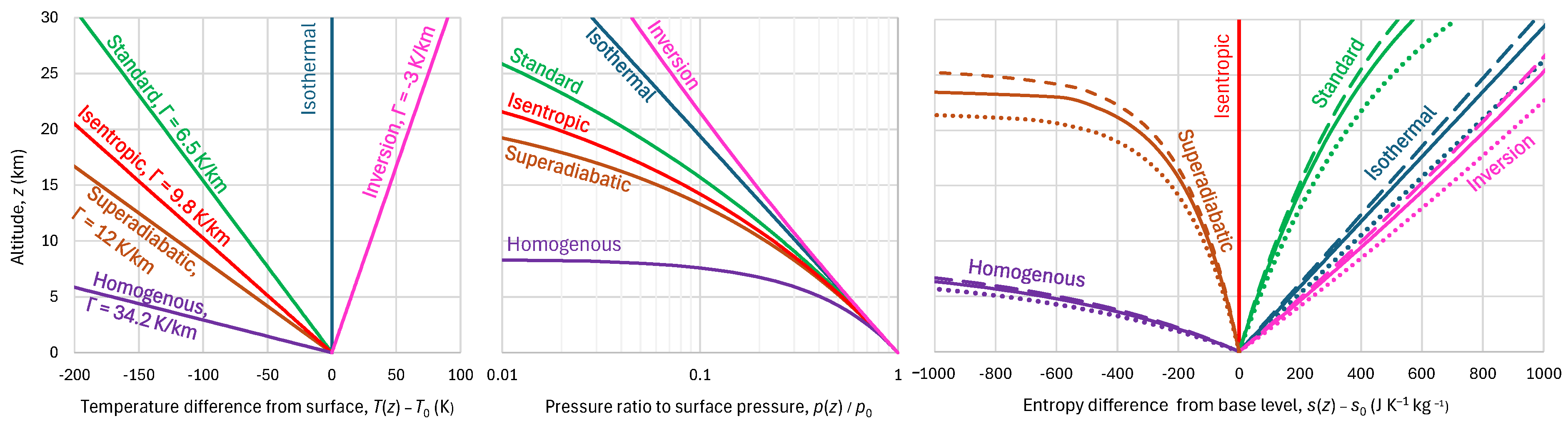
Figure 4.
(left) Lower troposphere profiles as observed by radiosondes at the indicated sites and dates. The slopes noted are calculated by linear regression on the points shown in the graph (not the entire range covered by radiosonde data). The profiles with continuous lines correspond to daytime and those with dashed lines to nighttime. For comparison, the standard atmospheric profile, as well as the slope of the isentropic profile are also shown. (Data retrieved from [27].)
Figure 4.
(left) Lower troposphere profiles as observed by radiosondes at the indicated sites and dates. The slopes noted are calculated by linear regression on the points shown in the graph (not the entire range covered by radiosonde data). The profiles with continuous lines correspond to daytime and those with dashed lines to nighttime. For comparison, the standard atmospheric profile, as well as the slope of the isentropic profile are also shown. (Data retrieved from [27].)
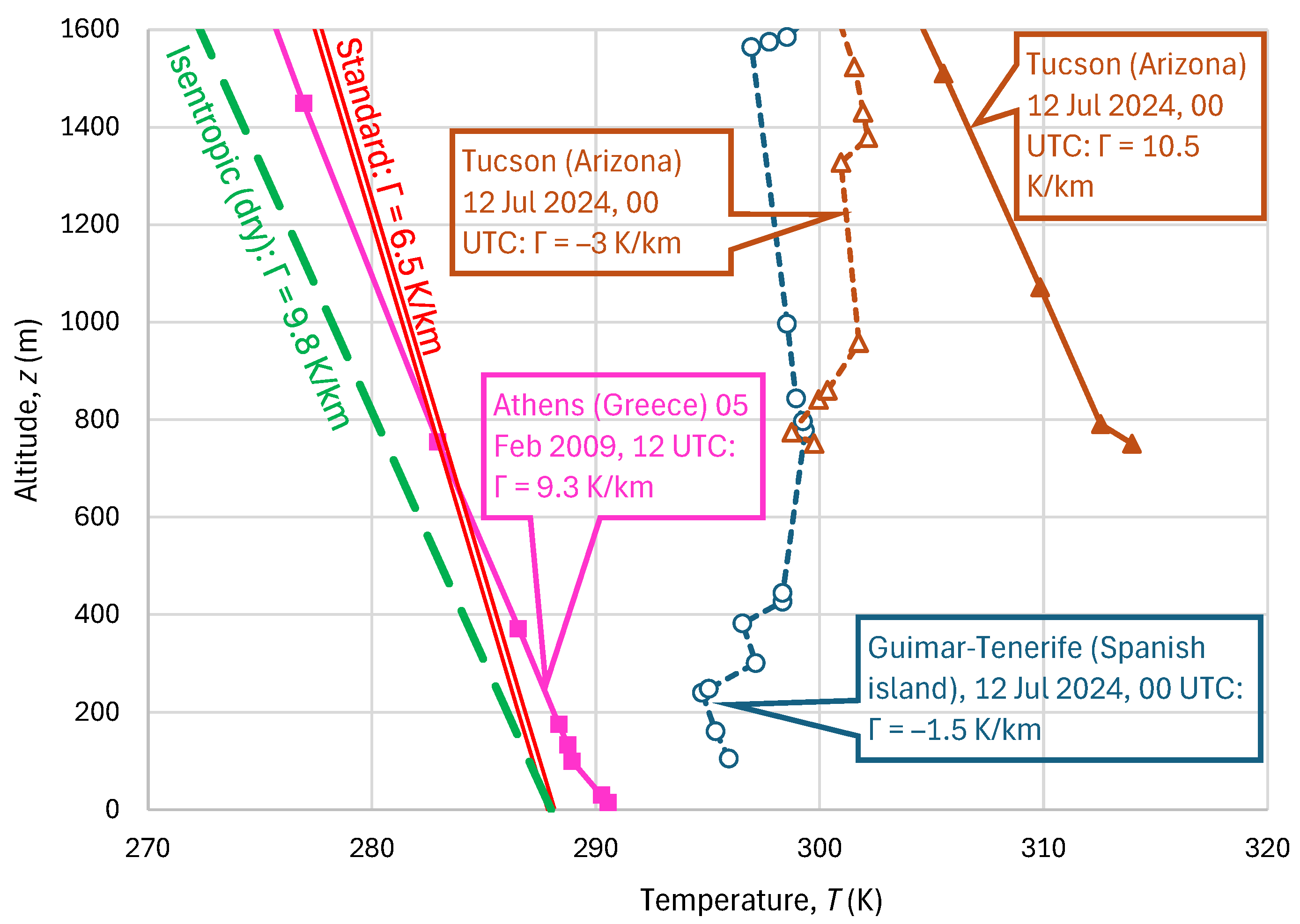
Figure 5.
Vertical wet isentropic temperature profiles in the atmosphere for the indicated surface temperatures. For comparison, the dry isentropic profile for one of the illustrated temperatures is also plotted. The lapse rate values near the surface are 4.8, 3.5 and 8.2 K/km for surface temperature of 288, 303 and 258 K, respectively.
Figure 5.
Vertical wet isentropic temperature profiles in the atmosphere for the indicated surface temperatures. For comparison, the dry isentropic profile for one of the illustrated temperatures is also plotted. The lapse rate values near the surface are 4.8, 3.5 and 8.2 K/km for surface temperature of 288, 303 and 258 K, respectively.
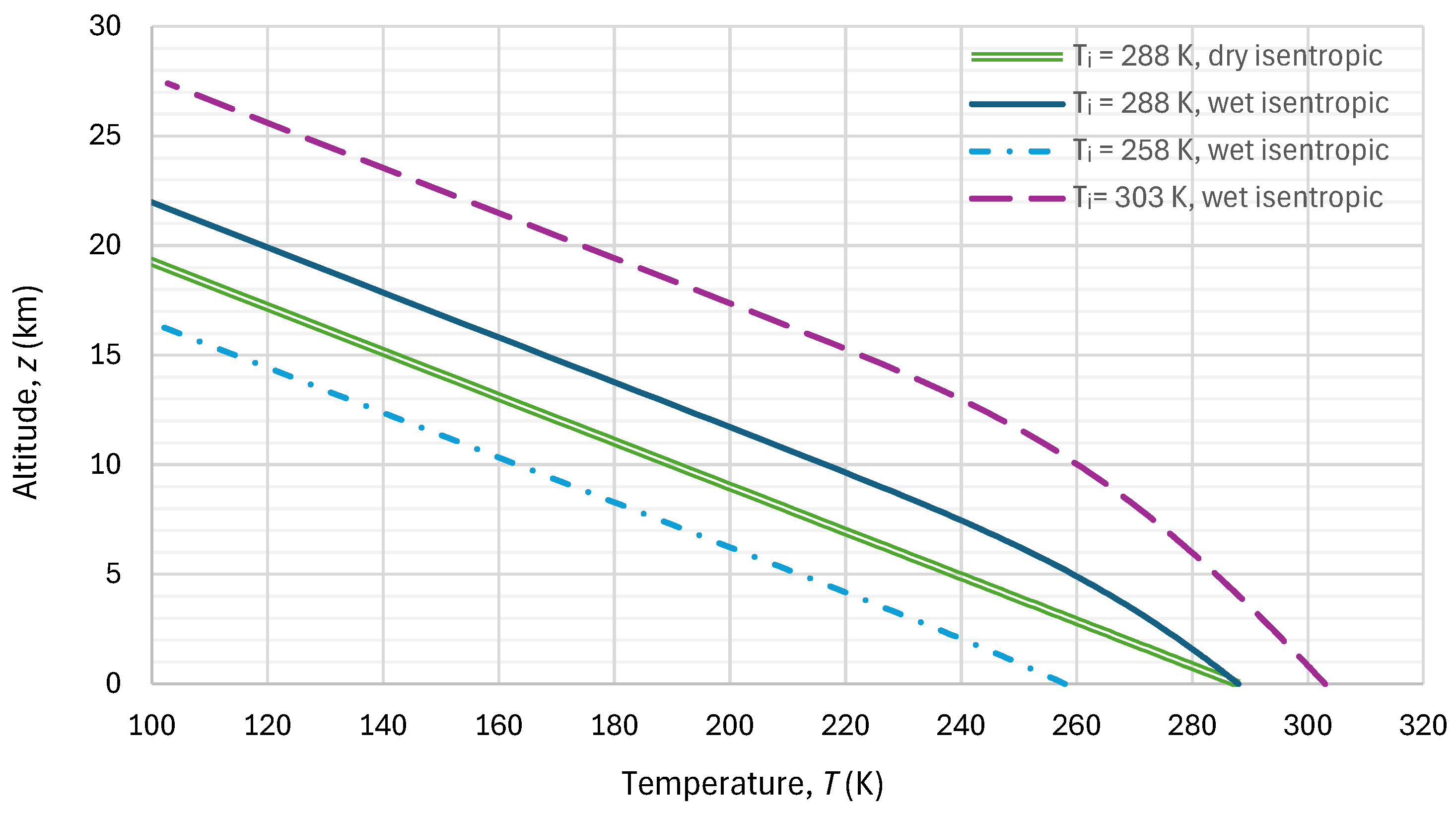
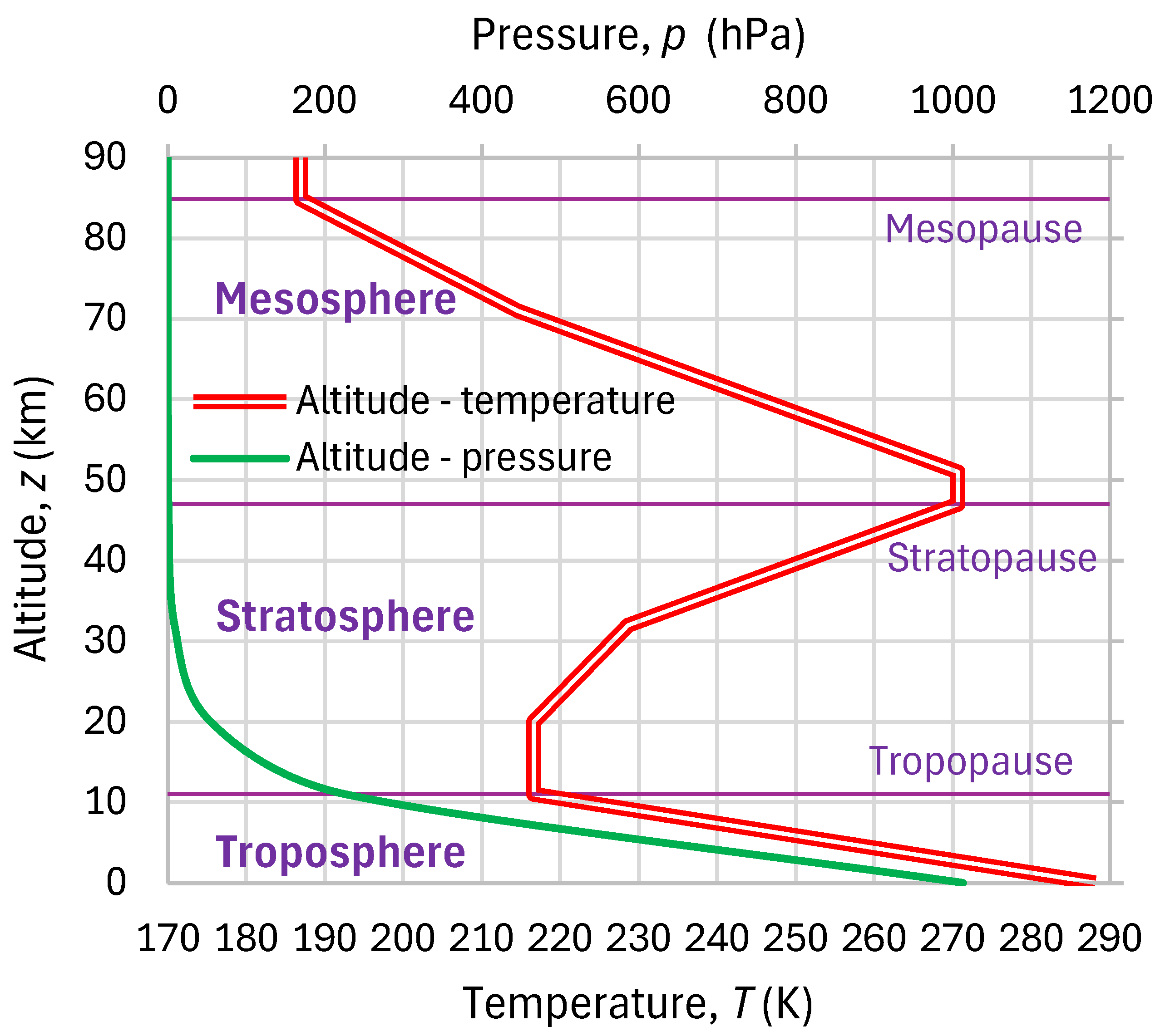
Figure 7.
ERA5 temperature (marked as “observed”) vs. ERA5 geopotential height, spatially integrated over ocean grid points at (upper row) a tropical zone extending ±7.5° around the equator and (lower row) a polar zone of width 7.5° south of the north pole, for mean monthly scale and specifically for the months of (left column) February and (right column) August. The monthly average profiles are compared to (a) the profile of the standard atmosphere (shifted to match the temperature at ), (b) the closest MODTRAN profile (namely the tropical profile for the upper row, and the subarctic winter and subarctic summer profiles for the left and right panels of the lower row, respectively), (c, d) the dry and moist isentropic profiles, respectively, and (e) the isothermal profile with the column average temperature.
Figure 7.
ERA5 temperature (marked as “observed”) vs. ERA5 geopotential height, spatially integrated over ocean grid points at (upper row) a tropical zone extending ±7.5° around the equator and (lower row) a polar zone of width 7.5° south of the north pole, for mean monthly scale and specifically for the months of (left column) February and (right column) August. The monthly average profiles are compared to (a) the profile of the standard atmosphere (shifted to match the temperature at ), (b) the closest MODTRAN profile (namely the tropical profile for the upper row, and the subarctic winter and subarctic summer profiles for the left and right panels of the lower row, respectively), (c, d) the dry and moist isentropic profiles, respectively, and (e) the isothermal profile with the column average temperature.
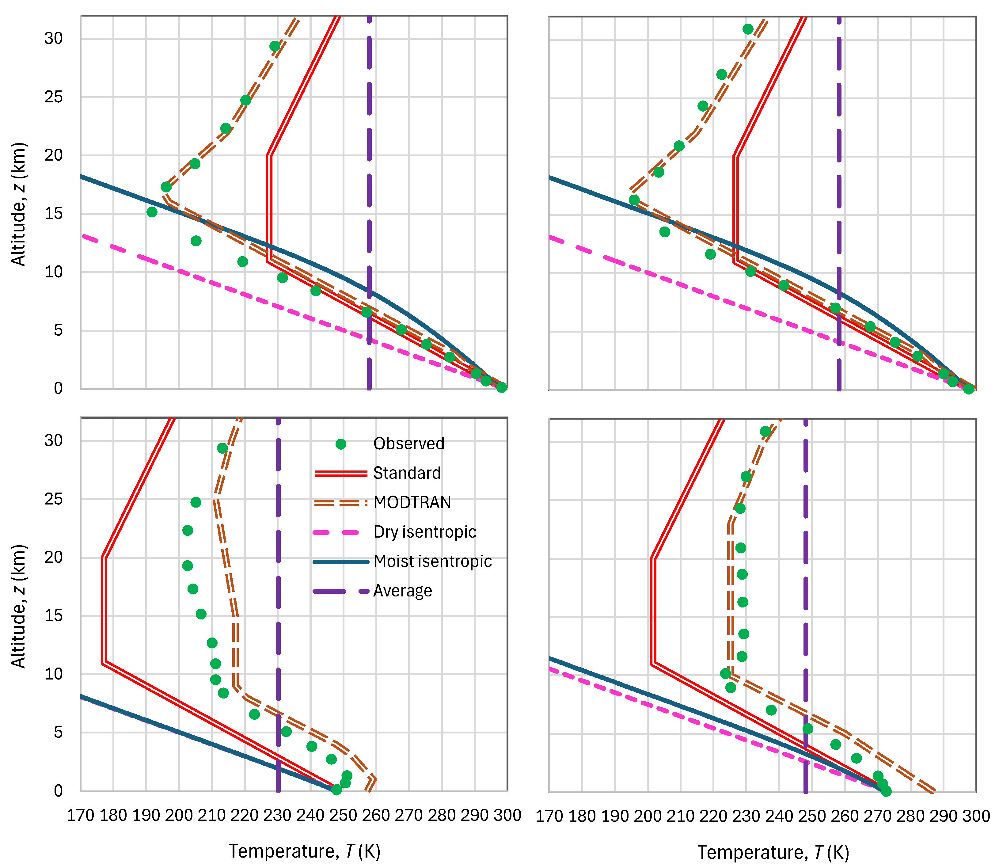
Figure 8.
Blackbody radiation intensity for the Sun’s surface (spectral radiant exitance, 5772 Κ, ) and Sun viewed from Earth (irradiance, for sr), in comparison to terrestrial (Earth’s) blackbody radiation (spectral radiant exitance, 255 Κ, ). Classification of radiation based on wavelength is also shown, with visible light defined between 0.4 and 0.7 μm and the boundary between solar (SW) and terrestrial (LW) radiation defined at a wavelength of 4 μm. The wavelengths at which the intensity is maximized are 0.502 μm and 11.36 μm for solar and terrestrial radiation, respectively. The temperature 255 Κ is the mean temperature of the Earth’s atmosphere (see section 4.3 for justification).
Figure 8.
Blackbody radiation intensity for the Sun’s surface (spectral radiant exitance, 5772 Κ, ) and Sun viewed from Earth (irradiance, for sr), in comparison to terrestrial (Earth’s) blackbody radiation (spectral radiant exitance, 255 Κ, ). Classification of radiation based on wavelength is also shown, with visible light defined between 0.4 and 0.7 μm and the boundary between solar (SW) and terrestrial (LW) radiation defined at a wavelength of 4 μm. The wavelengths at which the intensity is maximized are 0.502 μm and 11.36 μm for solar and terrestrial radiation, respectively. The temperature 255 Κ is the mean temperature of the Earth’s atmosphere (see section 4.3 for justification).
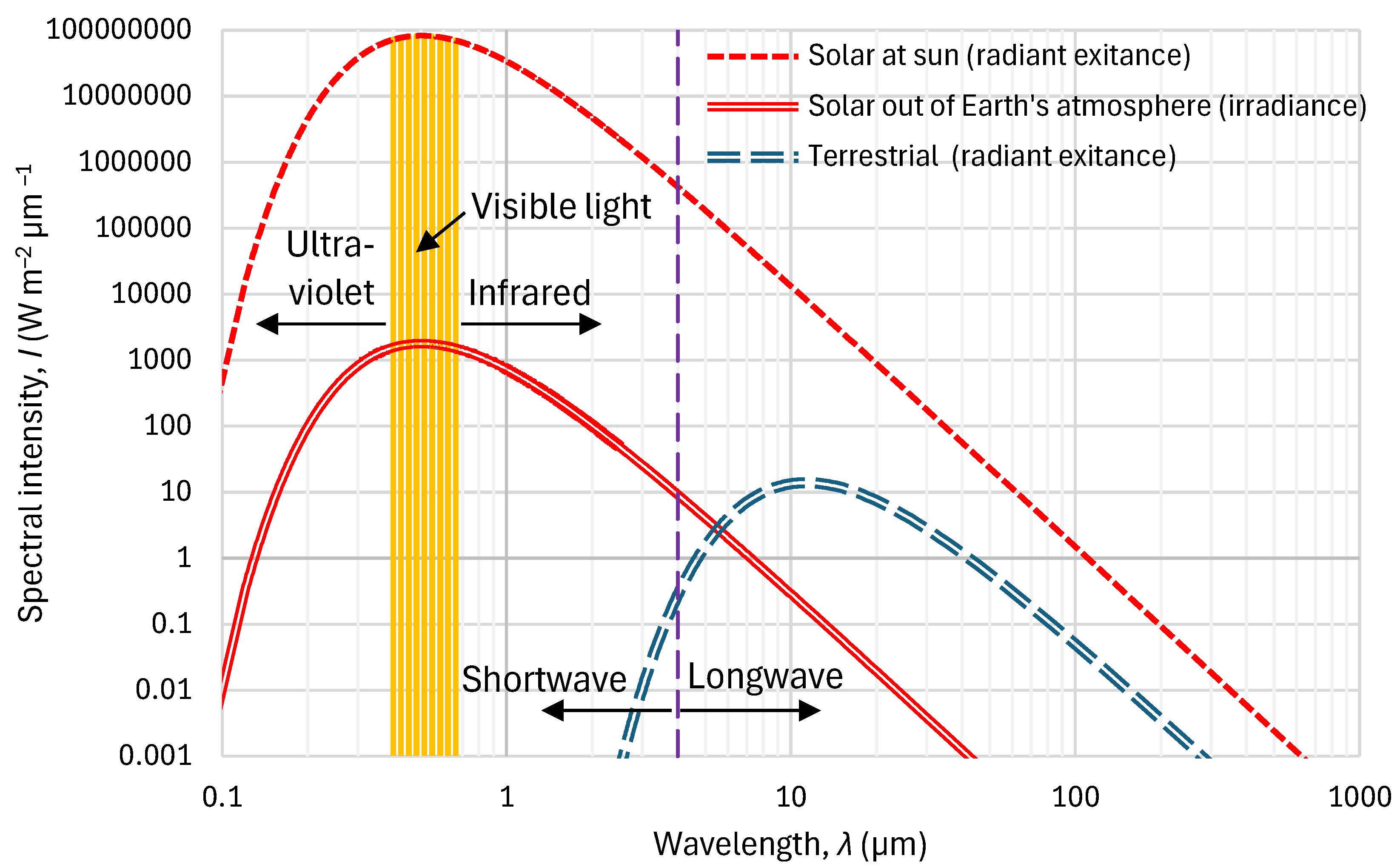
Figure 9.
Transmission and absorption of SW (solar) and LW (terrestrial) radiation through atmosphere, vs. wavelength. The absorption bands of Earth's atmosphere (middle) affect both downwelling solar radiation and upgoing LW radiation emitted near the surface (upper). The individual absorption spectra of radiatively active gases (plus Rayleigh scattering) are also shown (lower) (Source: [37] under a CC license.)
Figure 9.
Transmission and absorption of SW (solar) and LW (terrestrial) radiation through atmosphere, vs. wavelength. The absorption bands of Earth's atmosphere (middle) affect both downwelling solar radiation and upgoing LW radiation emitted near the surface (upper). The individual absorption spectra of radiatively active gases (plus Rayleigh scattering) are also shown (lower) (Source: [37] under a CC license.)
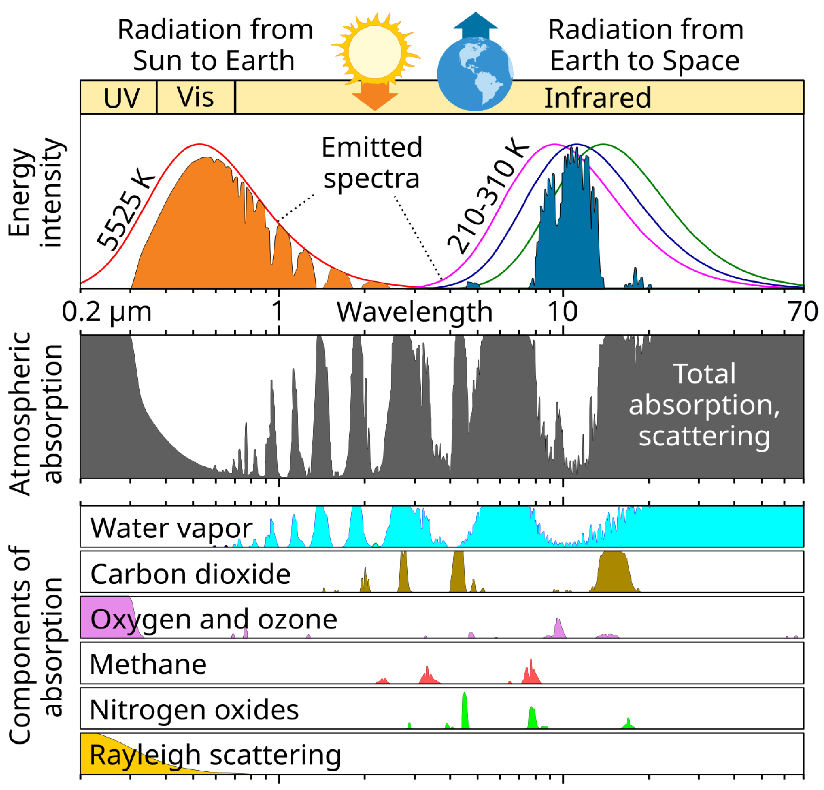
Figure 10.
Temperature variation at the atmospheric level of 500 hPa according to ERA5 Reanalysis. In addition to annual global average, maxima and minima are plotted as indicated in legend; the dotted line, almost indistinguishable from the line of annual average, is a linear trend with slope 0.14 K/decade. The data were retrieved from WRIT [34], except from the series of annual averages of monthly maxima and minima, which were retrieved from ClimExp [35].
Figure 10.
Temperature variation at the atmospheric level of 500 hPa according to ERA5 Reanalysis. In addition to annual global average, maxima and minima are plotted as indicated in legend; the dotted line, almost indistinguishable from the line of annual average, is a linear trend with slope 0.14 K/decade. The data were retrieved from WRIT [34], except from the series of annual averages of monthly maxima and minima, which were retrieved from ClimExp [35].
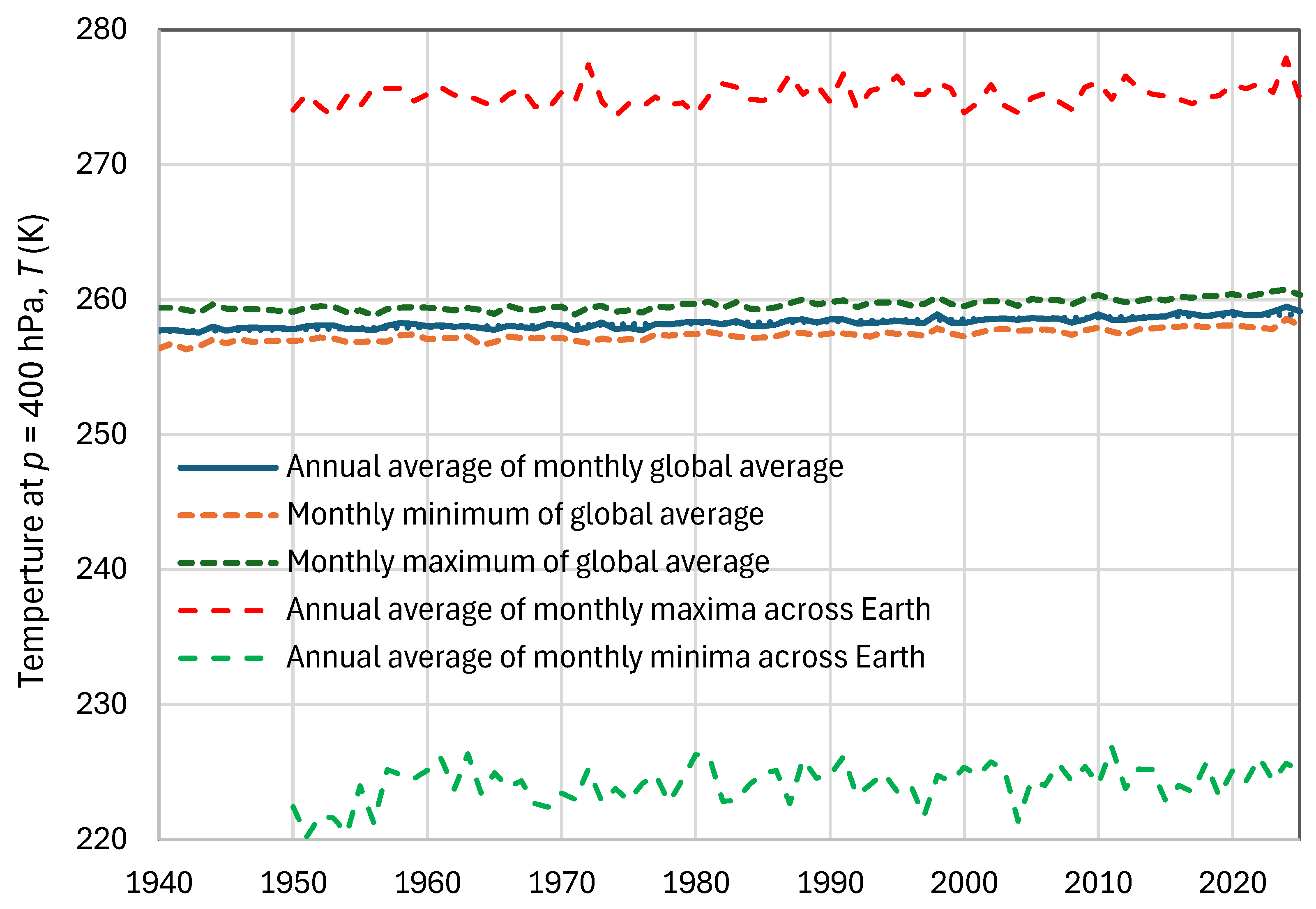
Figure 11.
Surface and TOA temperatures leading to energy balance vs. lapse rate, as calculated from RRTM runs using default parameters (without clouds).
Figure 11.
Surface and TOA temperatures leading to energy balance vs. lapse rate, as calculated from RRTM runs using default parameters (without clouds).
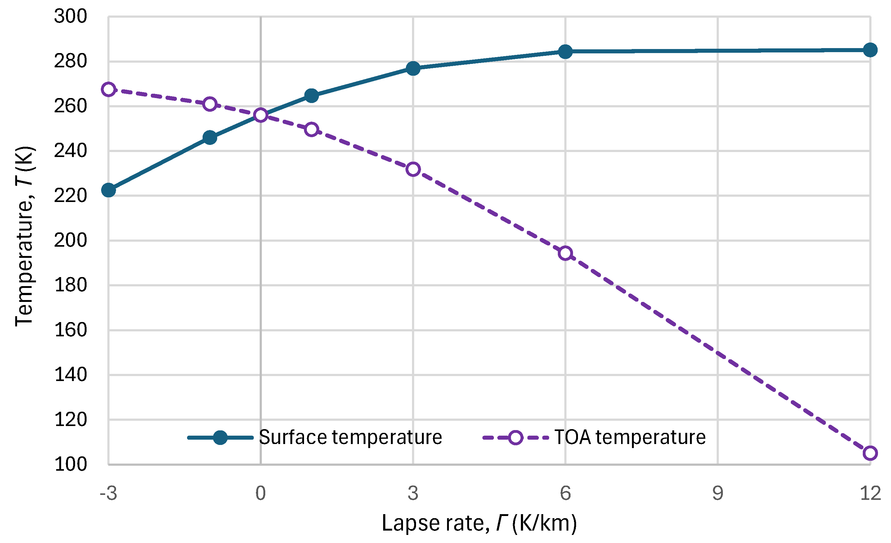
Figure 12.
Vertical distribution of net radiation flux gradient for the RRTM runs as in Figure 11 (assuring the energy balance) vs. lapse rate. For better presentation, smoothing of the original values was performed by taking moving averages over five adjacent values.
Figure 12.
Vertical distribution of net radiation flux gradient for the RRTM runs as in Figure 11 (assuring the energy balance) vs. lapse rate. For better presentation, smoothing of the original values was performed by taking moving averages over five adjacent values.
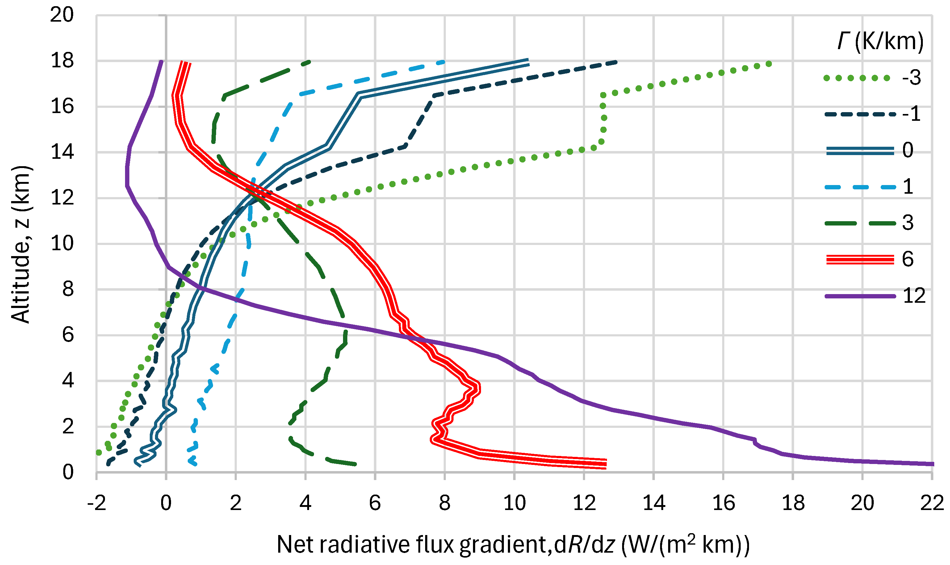
Figure 13.
Vertical radiation intensities at the top of the atmosphere observed with a Michaelson interferometer in a satellite (after Hanel and Conrath [48]), and modelled with radiation transfer theory for the Mediterranean and Antarctica. (Reproduction with adaptation of part of Figure 9 in [47].)
Figure 13.
Vertical radiation intensities at the top of the atmosphere observed with a Michaelson interferometer in a satellite (after Hanel and Conrath [48]), and modelled with radiation transfer theory for the Mediterranean and Antarctica. (Reproduction with adaptation of part of Figure 9 in [47].)
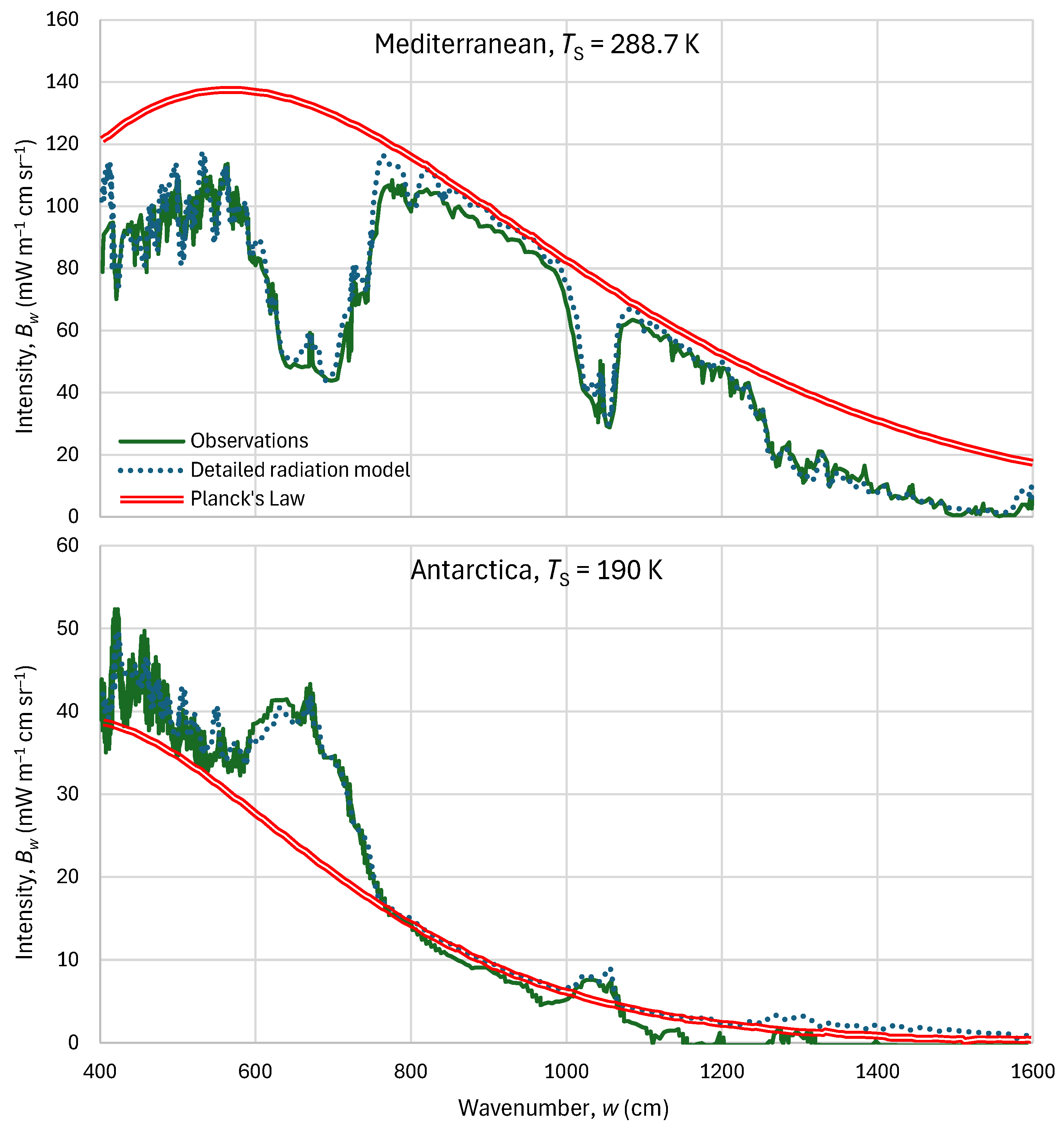

Table 1.
Gases appearing in Earth’s atmosphere in proportions (mole fraction) > 0.05%, and their characteristics as derived by our stochastic framework. Conventional experimental values for the isobaric specific heat are also given in the table and compared with theoretical values. (Trace gases not included in the table constitute <0.05% altogether.)
Table 1.
Gases appearing in Earth’s atmosphere in proportions (mole fraction) > 0.05%, and their characteristics as derived by our stochastic framework. Conventional experimental values for the isobaric specific heat are also given in the table and compared with theoretical values. (Trace gases not included in the table constitute <0.05% altogether.)
| Gas | Structure | Mole fraction (%)* | , kg/kmol |
, |
, | Experimental,† | % deviation | ||
|---|---|---|---|---|---|---|---|---|---|
| Nitrogen, N2 | Diatomic | 78.1 (77.8) | 5 | 28.014 | 296.8 | 742.0 | 1038.8 | 1040 | 0.1 |
| Oxygen, O2 | Diatomic | 21.0 (20.9) | 5 | 31.998 | 259.8 | 649.6 | 909.5 | 918 | 0.9 |
| Argon, Ar | Monatomic | 0.9 (0.9) | 3 | 39.950 | 208.1 | 312.2 | 520.3 | 522 | 0.3 |
| Water vapour, H2O | Triatomic, nonlinear | 0 (0.4)‡ | 6 | 18.015 | 461.5 | 1384.6 | 1846.1 | 1884 | 2.0 |
| Dry air | Mixture | 100 (100) | 4.98 | 28.958 | 287.1 | 721.1 | 1002.2 | 1004 | 0.2 |
- * The percentages without parentheses are for dry air and those in parentheses for moist air for the entire atmosphere.
- †The value given here for water vapour was taken from [25] for the triple point of water.
- ‡ It typically varies at 0–3%, averaging at 0.4%
Table 2.
Comparison of average Earth’s temperature resulting for the indicated assumptions and albedo
Table 2.
Comparison of average Earth’s temperature resulting for the indicated assumptions and albedo
| Case description | Ratio |
(K) for emissivity = | |||
|---|---|---|---|---|---|
| 1 | 0.95 | 0.9 | 0.85 | ||
| at a surface perpendicular to Sun’s rays | 1.000 | 359.2 | 363.8 | 368.7 | 374.0 |
| 0.707 | 254.0 | 257.2 | 260.7 | 264.5 | |
| Nonrotating planet (or rotating parallel to Sun’s rays) | 0.400 | 143.7 | 145.5 | 147.5 | 149.6 |
| Fast rotating planet without tilt | 0.699 | 251.0 | 254.3 | 257.7 | 261.5 |
| Fast rotating planet with Earth's tilt | 0.681 | 244.6 | 247.7 | 251.1 | 254.7 |
Disclaimer/Publisher’s Note: The statements, opinions and data contained in all publications are solely those of the individual author(s) and contributor(s) and not of MDPI and/or the editor(s). MDPI and/or the editor(s) disclaim responsibility for any injury to people or property resulting from any ideas, methods, instructions or products referred to in the content. |
© 2026 by the authors. Licensee MDPI, Basel, Switzerland. This article is an open access article distributed under the terms and conditions of the Creative Commons Attribution (CC BY) license (http://creativecommons.org/licenses/by/4.0/).
Copyright: This open access article is published under a Creative Commons CC BY 4.0 license, which permit the free download, distribution, and reuse, provided that the author and preprint are cited in any reuse.


