

Submitted:
28 June 2026
Posted:
30 June 2026
You are already at the latest version
Abstract
Accurate nighttime land surface temperature (LSTn) forecasting in data-scarce, topographically complex regions remains a significant challenge for satellite remote sensing and climate monitoring. To address this, the present study introduces the Physics-Guided Transformer Bidirectional Long Short-Term Memory (PG-ST-BiLSTM) deep learning model. For comparison, we employ four baseline models: three deep learning models (TCN, LSTM, and BiLSTM) and one statistical model (linear regression). Using Afghanistan, a topographically challenging and data-scarce region, as a “hard” test bed, the proposed model is evaluated across five major river basins over the period 2001-2024. The proposed PG-ST-BiLSTM achieves an R² of 0.977, RMSE of 2.023 °C, and MAE of 1.534 °C, outperforming baseline models including TCN (R² = 0.961), LSTM (R² = 0.966), BiLSTM (R² = 0.966), and linear regression (R² = 0.926). The model demonstrates strong alignment between observed and fitted LSTn values along the reference line of y = 0.98x + 0.21 closely approaching the 1:1 reference line. All Sen’s slope values are positive, confirming a universal nighttime warming trend across the projected period (2025-2040), with a grand mean of +0.0160 °C/year across all basin-season combinations, suggesting a marginal acceleration of LSTn warming under a trend-stationary climatological assumption, wherein historical warming rates derived from Mann-Kendall and Theil–Sen analyses are assumed to persist through 2040. At the seasonal level, Winter exhibits the highest projected warming rate (+0.1174 °C/year), followed by Summer (+0.0984 °C/year), Autumn (+0.0545 °C/year), and Spring (+0.0504 °C/year), indicating that cold-season and peak-summer nighttime temperatures are projected to remain the most thermally vulnerable through 2040. At the basin level, the hyper-arid Helmand Basin records the highest projected mean Sen’s slope (+0.0796 °C/year), consistent with its minimal vegetation buffering and high nocturnal thermal emissivity, while the Amu-Darya Basin exhibits the lowest warming rate (+0.0460 °C/year), attributable to orographic cooling and comparatively higher soil moisture retention. These results demonstrate the generalizability and reproducibility of the PG-ST-BiLSTM model for nighttime LST forecasting in data-scarce, mountainous regions, with direct relevance to climate adaptation, water resource planning, and cryosphere monitoring worldwide.
Keywords:
LST
; PG-ST-BiLSTM
; transformer
; physics-guided deep learning
; Afghanistan
; LSTn
; MODIS
1. Introduction
Land surface temperature (LST) is a fundamental geophysical variable that regulates land–atmosphere interactions, surface energy balance, hydrological processes, and ecosystem dynamics [1]. In the context of accelerating global warming, accurate monitoring and forecasting of LST have attracted growing attention from both the scientific community and operational climate-management agencies [2]. Within this body of research, daytime LST has been shown to respond strongly to instantaneous solar radiation and short-term surface conditions, whereas nighttime LST (LSTn) more directly reflects land-surface thermal inertia, subsurface heat storage, and background atmospheric stability [3]. Reliable LSTn forecasting is therefore particularly valuable for climate assessment, environmental risk evaluation, and the design of adaptation strategies in climatically vulnerable regions [4]. A wide range of traditional statistical and deep learning techniques has been employed in the related literature to identify the dominant drivers of LSTn and to forecast its spatiotemporal fluctuations. Traditional approaches, including Multiple Linear Regression (MLR), Geographically Weighted Regression (GWR), Autoregressive Integrated Moving Average (ARIMA), Seasonal ARIMA (SARIMA), Support Vector Regression (SVR), Random Forest (RF), Extreme Gradient Boosting (XGBoost), and the Mann-Kendall trend test coupled with Sen’s slope estimator—have been widely applied to characterize long-term LSTn trends and to quantify the influence of biophysical and climatic covariates [5,6]. More recently, deep learning (DL) architectures have demonstrated superior capability in capturing the nonlinear and spatiotemporal dependencies inherent in LST dynamics. Notable examples include Artificial Neural Networks (ANN), Long Short-Term Memory (LSTM) networks, Bidirectional LSTM (BiLSTM), Gated Recurrent Units (GRU), Convolutional Neural Networks (CNN), ConvLSTM, Transformer-based models, and hybrid frameworks such as CNN-LSTM and Transformer-LSTM, which integrate spatial feature extraction with temporal sequence modeling to enhance forecasting accuracy [7,9]. Among these DL techniques, Physics-guided Spatio-temporal Bidirectional LSTM (PG-ST-BiLSTM) has emerged as a promising approach in which domain knowledge is embedded into data-driven architectures to improve predictive consistency [10,11]. Therefore, this study employs PG-ST-BiLSTM to systematically evaluate the accuracy of the selected method on historical data spanning from 2001 to 2024, and subsequently to forecast LSTn from 2025 to 2040 using monthly data from Afghanistan.
To realize this forecasting framework, the methodological workflow typically encompasses several interdependent stages, including the acquisition of LSTn and environmental driver datasets, time-series preprocessing and feature construction, development and training of the forecasting model, generation of temporal predictions, and subsequent validation [12,13]. Considerable effort has been devoted to the construction and optimization of statistical and DL models for LSTn estimation and forecasting. For instance, LSTM- and Transformer-based architectures have been refined through hyperparameter tuning and cross-validation strategies to enhance temporal accuracy [14,15], while advanced optimization techniques such as Bayesian optimization, adaptive learning-rate scheduling, and regularization have been adopted to improve model stability and generalization in environmental time-series applications [16,17].
However, these model-centric improvements are only one side of the forecasting pipeline. Equally critical-yet far less systematically addressed-is the design of the temporal input dataset itself. In many cases, the length of the input sequence, the representation of seasonal cycles, and the integration of multivariate environmental drivers are selected empirically rather than through principled evaluation. Short input windows may fail to capture full seasonal periodicity, whereas excessively long sequences may introduce noise and unstable gradient propagation [18,19]. Similarly, the temporal alignment and joint representation of LSTn with vegetation, precipitation, and soil moisture drivers are often implemented without explicit consideration of cross-seasonal thermal persistence. As a result, models tend to learn short-term correlations while underrepresenting the multi-month memory effects that govern nighttime surface thermal dynamics. Moreover, most forecasting frameworks rely on pointwise loss functions that optimize prediction error independently at each time step, without constraining the continuity of month-to-month temperature transitions [20].
Despite these advances, existing studies have predominantly emphasized architectural refinement and parameter optimization [21,22], yet the systematic design of the temporal input dataset including feature selection, gap-filling, and temporal alignment-has received limited attention, especially in data-sparse regions such as Afghanistan. This limitation is particularly problematic in regions characterized by strong elevation gradients and nonlinear seasonal variability, where physically inconsistent forecasts can readily emerge due to the neglect of terrain-driven thermal dynamics. Consequently, despite ongoing improvements in model architecture and hyperparameter optimization, achieving temporally coherent and physically consistent nighttime LSTn forecasting across complex mountainous environments remains a significant challenge.
Many of the limitations identified above stem from methodological choices that are made empirically rather than through systematic evaluation, introducing avoidable uncertainty into LSTₙ predictions [5,8]. Although uncertainty in satellite-based LSTn forecasting has attracted increasing attention in recent years, existing studies have typically examined individual sources of variability in isolation. Preprocessing decisions-including quality-control filtering, temporal aggregation (e.g., 8-day to monthly composites), and gap-filling of cloud- or snow-flagged Moderate Resolution Imaging Spectroradiometer (MODIS), observations have been shown to alter the multi-month thermal signal that the model is required to learn [5,6,8,23], while spatial resolution and resampling strategies further affect the representation of thermal gradients in heterogeneous mountainous regions [24,25]. Equally important, the configuration of temporal inputs and environmental drivers, including input-window length, seasonal representation, and multivariate driver integration, is often determined through prior experience or trial-and-error, even though spatial heterogeneity and strong elevation, climate gradients, such as those characterizing Afghanistan, mean that a configuration well suited to one basin may be suboptimal in another [18,19,26]. At the architectural level, recurrent and convolutional networks cannot, on their own, prioritize the distant temporal dependencies that govern cross-seasonal nocturnal thermal memory; Transformer-based attention has been introduced to overcome this limitation [27], and BiLSTM architectures have been shown to improve bidirectional contextual learning across seasonal cycles [28,29]. Nevertheless, no prior study has systematically benchmarked a comprehensive set of DL architectures, including Temporal Convolutional Networks (TCN), Long Short-Term Memory (LSTM), and Bidirectional LSTM (BiLSTM), against a PG-ST-BiLSTM within a unified LSTn forecasting framework.
By effectively addressing these limitations, this study makes several key contributions to the literature. First, this study proposes the PG-ST-BiLSTM framework-a unified pipeline that integrates temporal input design, a hybrid Transformer-BiLSTM architecture, and a physics-guided training objective to improve both the predictive accuracy and physical consistency of LSTn forecasting in data-scarce mountainous environments. Second, three environmental drivers are employed as predictors, including NDVI, precipitation (PREC), and soil moisture (SM), selected for their collective capacity to capture vegetation phenology, atmospheric water input, and subsurface thermal inertia, which are the dominant processes governing nocturnal surface energy exchange in Afghanistan’s continental climate. Third, rather than optimizing a single model in isolation, this study systematically evaluates three methodological factors that are typically treated independently in the literature: (1) the configuration of the temporal input window and multivariate driver representation; (2) the integration of Transformer-based long-range attention with bidirectional recurrent seasonal learning; and (3) the incorporation of a physics-motivated temporal smoothness constraint directly into the loss function. Each factor is evaluated against four baselines, including TCN, LSTM, BiLSTM, and Linear Regression, under identical data partitions and preprocessing conditions, enabling performance differences to be attributed to specific design choices rather than to data or implementation variation. Finally, the novelty of PG-ST-BiLSTM lies in its principled integration of components, which can be articulated through three distinct contributions that substantively differentiate this study from prior work: (1) the first controlled benchmarking of TCN, LSTM, BiLSTM, and PG-ST-BiLSTM on LSTn, providing direct empirical evidence of which architectural choices matter most; (2) a physics-motivated smoothness constraint derived from land-surface thermal inertia principles, demonstrated through ablation to contribute more to predictive accuracy than either the Transformer encoder or the multi-driver input set; and (3) the first basin-disaggregated, season-stratified nighttime warming projections through 2040 for Afghanistan, a region characterized by extreme topographic and climatic heterogeneity, near-zero ground-based monitoring infrastructure, and high practical stakes for water resource planning, agricultural risk assessment, and cryosphere monitoring.
2. Study area and data sources
2.1. Study area
This study performs spatially heterogeneous LSTn forecasting across the five major river basins of Afghanistan, including Amu Darya, Harirud–Murghab, Helmand, Kabul, and Northern. Afghanistan is located in south-central Asia between 29°-38° N and 61°-74° E (Figure 1) [32]. The country covers approximately 652,000 km² and exhibits substantial topographic variability, with elevations ranging from approximately 230 m in the southwestern lowlands to 7,471 m in the Hindu Kush Mountains in the northeast. This pronounced elevational gradient generates strong climatic contrasts across relatively short horizontal distances: northeastern high-altitude regions experience cold winters and comparatively high annual precipitation, whereas the southern lowlands are characterized by hot, arid conditions with limited rainfall. Hydrologically, the country is drained by five aforementioned major river basins, each exhibiting distinct hydroclimatic regimes [33,34]. The combined spatial heterogeneity in elevation, climate, and land cover gives rise to complex nocturnal surface thermal dynamics, making Afghanistan a particularly informative setting in which to investigate LSTn variability for regional climate assessment and environmental management [35,36].
2.2. Nighttime Land Surface Temperature Dataset
The LSTn data constitute the primary variable analysed in this study. LSTn was derived from the MODIS MOD11A2 Collection 6.1 product acquired from the Terra satellite platform [37]. This dataset provides 8-day composite LSTn observations at a spatial resolution of 1 km for the period 2001–2024 [38]. The LST_Night_1km band was selected to represent nocturnal surface thermal conditions. MODIS LST digital numbers were converted to degrees Celsius using the standard scale factor: . Quality control filtering was applied using the QC_Night band to remove cloud-contaminated and low-quality pixels. Pixels flagged as good quality under the mandatory QA bits and acceptable LST error conditions were retained for analysis. A total of 1,103 valid 8-day composite images were processed for the study period. The mean and trend of LSTn, NDVI, SM, and PREC are visualized in Figure 2(a)-2(h), respectively.
2.3. Environmental Driver Datasets
Based on previous studies of land–atmosphere interactions and surface energy balance processes, and considering data availability and consistency over the study period, three environmental driver datasets were incorporated into the analysis. An overview of the datasets is provided in Table 1.
2.4. Vegetation Index (NDVI)
Vegetation dynamics were represented using the MODIS MOD13Q1 Collection 6.1 Normalized Difference Vegetation Index (NDVI) product. This dataset provides 16-day composite observations at 250 m spatial resolution for 2001–2024 [39]. NDVI captures vegetation greenness and canopy activity, which influence surface energy partitioning and nocturnal cooling behaviour [41]. The NDVI data were resampled to 1 km resolution to match the MODIS LST grid.
2.5. Precipitation
Precipitation data were obtained from the Climate Hazards Group InfraRed Precipitation with Station data (CHIRPS) dataset. CHIRPS provides daily rainfall estimates at approximately 0.05° (~5.5 km) spatial resolution for the study period [42]. Daily precipitation values were aggregated into monthly totals and subsequently resampled to the 1-km LST grid. Precipitation is a key climatic driver that influences soil moisture conditions, vegetation growth, and surface thermal properties [43,44].
ECMWF Reanalysis v5 (ERA5) reanalysis was considered as an alternative source for both precipitation and soil moisture. However, CHIRPS was preferred over ERA5 precipitation for three reasons: (1) CHIRPS merges satellite-derived infrared estimates with quality-controlled ground station data, making it more accurate than pure reanalysis in data-sparse regions such as Afghanistan where ERA5’s precipitation fields are poorly constrained by in-situ observations [45]; (2) CHIRPS provides a higher native spatial resolution (~5.5 km vs ERA5’s ~31 km) [46], which better captures the orographic precipitation gradients characteristic of Afghanistan’s mountainous terrain; and (3) CHIRPS has been independently validated as the most reliable gridded precipitation product for Central Asia and the Hindu Kush region in multiple benchmark studies [47,48]. Similarly, FLDAS NOAH01 was preferred over ERA5 soil moisture because FLDAS assimilates CHIRPS precipitation as its forcing input, ensuring internal consistency between the precipitation and soil moisture fields used in this study, a consistency that would be compromised if ERA5 soil moisture were paired with CHIRPS precipitation.
2.6. Soil Moisture (0–10 cm)
Near-surface soil moisture data were derived from the FLDAS (NOAH01 V001) dataset. This product provides monthly soil moisture estimates for the 0–10 cm soil layer at approximately 0.1° (~11 km) spatial resolution for 2001-2024 [49]. Soil moisture strongly affects land surface thermal inertia and nocturnal heat storage capacity [50]. The data were spatially resampled to the 1-km LST grid to ensure consistency with other variables.
3. Methodology
3.1. PG-ST-BiLSTM Framework and Key Steps for LSTn Modeling
The common nighttime LST forecasting framework generally includes the following processes (Figure 3): (1) obtain satellite-derived LST data and associated environmental driver datasets; (2) conduct systematic data preprocessing and feature construction; (3) transform the time series into supervised learning sequences; (4) select appropriate forecasting models to construct the prediction framework; (5) perform short- to medium-range forecasting; and (6) evaluate prediction accuracy and quantify forecast uncertainty using statistical metrics. Each of these steps may introduce methodological uncertainty if a single modeling configuration is subjectively selected.
Therefore, this study proposes a structured Physics-Guided Spatio-Temporal LSTM (PG-ST-LSTM) framework to ensure methodological robustness and physical consistency (Figure 4) [9,51]. First, LSTn and associated environmental drivers were obtained from MODIS MOD11A2 Collection 6.1 (8-day, 1 km; 2001-2024). Three predictor variables were integrated: NDVI (MOD13Q1), precipitation (CHIRPS), and near-surface soil moisture (FLDAS NOAH01). These variables represent vegetation dynamics, hydrological forcing, and surface moisture conditions influencing nocturnal thermal behaviours [42,43,49,50]. Second, data preprocessing was performed to ensure spatial and temporal consistency. MODIS QA flags were applied to remove cloud-contaminated pixels [52]. The 8-day LST composites were aggregated to monthly means, and all ancillary datasets were resampled to the 1 km grid. Basin-level zonal statistics and seasonal (DJF, MAM, JJA, SON) averages were computed. All predictors were normalized using Min-Max scaling to stabilize model training. Third, the multivariate time series was converted into supervised learning sequences using a 12-month sliding window to capture the annual thermal cycle.
Each input vector comprised six features: LSTn, NDVI, precipitation, soil moisture, and cyclic seasonal encodings (sin, cos). For the validated short-to-medium horizon (2015-2024), this direct multi-output strategy avoids recursive error accumulation by predicting all four steps simultaneously. For the long-range projection period (2025-2040), an autoregressive rolling strategy was employed, wherein the model’s four-step output is appended to the input sequence and the window is advanced by one step iteratively.
This transition is deliberately conservative: the direct strategy is used where ground-truth comparison is possible, while the autoregressive strategy is adopted only for the projection horizon where no observed data exist for verification, with forecast uncertainty explicitly quantified through the confidence-tier framework described in Section 3.4, and chronological partitioning (2001-2014 training; 2015-2024 validation) was applied to prevent temporal leakage. Fourth, suitable forecasting models were implemented to construct the prediction framework. In addition to four baselines (LR, LSTM, BiLSTM, TCN), the proposed PG-ST-LSTM model was developed.
The architecture integrates a dual-block Transformer encoder for long-range temporal attention, stacked Bidirectional LSTM layers for sequential learning, and a physics-guided temporal smoothness constraint within the loss function to enforce physically plausible trajectories. The ‘spatio-temporal’ designation in PG-ST-BiLSTM refers to the framework’s simultaneous operation across five spatially distinct river basins under a unified modeling protocol, wherein basin identity is encoded implicitly through basin-specific input sequences rather than through explicit spatial convolution or graph-based spatial attention.
This is consistent with the use of ‘spatio-temporal’ in multi-site time series forecasting studies [53,54], where the term denotes joint modeling across spatial units rather than pixel-level spatial feature extraction. Readers seeking explicit spatial convolution should note that the basin-level aggregation performed during preprocessing converts the 2D spatial domain into a set of representative time series, making pixel-level CNN-based spatial processing neither necessary nor appropriate for this forecasting task.
Fifth, short- to medium-range forecasting was conducted using direct multi-output prediction to avoid recursive error accumulation. The model was trained using the Adam optimizer with early stopping and learning rate decay. Validation was performed on the independent 2015-2024 period to assess temporal generalization.
Sixth, prediction accuracy and uncertainty were quantified using R², RMSE, and MAE. Seasonal performance was examined to evaluate robustness under varying climatic conditions. Ablation experiments were conducted to isolate the contributions of the Transformer encoder, environmental drivers, and physics-guided regularization. Forecast degradation was assessed empirically (0.069 °C/year), forming the basis for confidence-tier classification in long-range projections. Mann–Kendall and Sen’s slope analyses were subsequently applied to derive statistically robust trend-constrained projections beyond the validated forecasting horizon [55,56].
3.2. Dataset Preparation for LSTn Modeling
3.2.1. Multicollinearity Assessment
The assessment of multicollinearity among environmental predictors is an important step in LST forecasting, particularly for regression-based baselines and correlation analysis. Multicollinearity arises when predictor variables exhibit strong interdependence, such that variation in one variable is systematically associated with variation in another. This redundancy may lead to unstable coefficient estimation, reduced interpretability, and inflated variance in linear modeling frameworks.
To ensure the statistical independence of the input predictors and to avoid redundancy in the DL model, the Variance Inflation Factor (VIF) was computed for each LSTn predictor following [57,58]. The VIF is defined as:
where represents the coefficient of determination obtained by regressing the predictor against all remaining predictors. The reciprocal term , referred to as tolerance, provides an equivalent measure of collinearity. A VIF value exceeding commonly accepted thresholds (e.g., VIF > 5 or 10) indicates potential multicollinearity [59]. Only predictors satisfying acceptable VIF criteria were retained for regression-based baseline modeling and driver analysis. Although DL architectures such as PG-ST-LSTM are generally less sensitive to multicollinearity due to nonlinear representation learning, this assessment ensures statistical robustness and interpretability in baseline comparisons and correlation analyses.
3.2.2. Temporal Feature Construction for Continuous Predictor Variables
Feature representation in LST forecasting requires careful design to capture the nonlinear relationship between environmental drivers and nighttime temperature. Unlike traditional regression-based discretization approaches, this study employs continuous predictor variables processed through engineered temporal encodings. Rather than dividing predictors into discrete intervals, seasonal periodicity is explicitly encoded using cyclical sine and cosine transformations.
The input feature representation consists of six continuous variables:
- ➢
- LSTn (target variable);
- ➢
- NDVI (vegetation state);
- ➢
- Precipitation (hydrological forcing)
- ➢
- Soil moisture (surface moisture availability);
- ➢
- Sine-transformed month (seasonal phase);
- ➢
- Cosine-transformed month (seasonal phase).
The cyclical encoding is formulated as:
This approach preserves annual thermal continuity, ensures December and January are treated as adjacent, and eliminates artificial discontinuities inherent in discrete interval methods. All predictors were normalized using Min-Max scaling to the [0,1] range, standardizing gradient magnitudes, and ensuring numerical stability during training [60,61].
3.2.3. Pearson Correlation and Driver Association Analysis
To quantify the biophysical influences on nighttime LST, Pearson correlation coefficients were computed between monthly basin-mean LSTn and the three environmental drivers (NDVI, precipitation, and soil moisture). The Pearson correlation coefficient measures the linear association strength between two variables and is formulated as [62]:
Correlations were assessed both annually and by season (DJF, MAM, JJA, SON) to identify whether driver–LSTn relationships vary across the annual cycle. A correlation coefficient magnitude exceeding a threshold of r > 0.7 indicates a strong association, while r < 0.3 suggests weak influence. Analyses were conducted over the complete 2001-2024 time series (n = 288 months) and tested for statistical significance at p < 0.05. Following Pearson analysis, multiple linear regression was applied to quantify the combined explanatory power of the three drivers:
The resulting seasonal R² values serve as a linear predictability baseline against which PG-ST-LSTM nonlinear performance is compared. This enables quantification of the performance gain achievable through deep learning architectures.
3.2.4. Sequence Construction and Chronological Sample Partitioning
To prevent information leakage from future observations into model training, strict chronological partitioning was applied. The complete 2001-2024 time series (288 months) was divided as follows:
Training period: January 2001- December 2014 (156 input-output sequence pairs)
Validation period: January 2015 - December 2024 (116 sequence pairs)
A sliding-window approach with a step size of one month was employed to construct sequinces, such that consecutive sequences overlap by 11 input months. Each sequence consists of a 12-month input window and a 4-month direct output vector. This 12-month input window provides the model with one complete annual thermal cycle, the dominant mode of LSTn variability in Afghanistan’s continental climate. The dataset imbalance was avoided by maintaining consistent sample representation across seasons. Both training and validation periods span multiple complete years, ensuring representative seasonal coverage in both subsets.
3.3. Machine Learning Models for Nighttime LST Forecasting
3.3.1. Linear Regression
Linear Regression (LR) serves as a fundamental baseline in this study. LR models the relationship between predictors and the target variable through a linear function [63]:
where are regression coefficients and are predictor variables. Despite its simplicity, LR provides interpretable coefficient estimates and establishes a minimal performance benchmark. Limitations include its inability to capture nonlinear temporal dependencies and interactions among environmental drivers. LR serves as the lower-bound baseline for assessing deep learning performance gains.
3.3.2. Long Short-Term Memory (LSTM)
The Long Short-Term Memory (LSTM) [64] It is a recurrent neural network architecture designed to capture temporal dependencies in sequential data. Unlike standard feedforward networks, LSTM maintains hidden states across time steps and employs gating mechanisms [65] to regulate information flow:
Te forget gate , input gate , and output gate control the flow of information. LSTM effectively captures long-range temporal patterns and has demonstrated success in time-series forecasting. However, standard unidirectional LSTM lacks explicit mechanisms for attending to long-range temporal dependencies across the input window.
3.3.3. Bidirectional LSTM (BiLSTM)
Bidirectional LSTM [29,66] processes sequences in both forward and backward directions, enabling the model to exploit contextual information from both past and future observations within the input window:
This bidirectional context is particularly valuable for capturing asymmetric warming and cooling transitions in continental climates. BiLSTM improves upon unidirectional LSTM by leveraging information from the complete input sequence. However, it still lacks explicit long-range attention mechanisms for prioritizing distant temporal relationships.
3.3.4. Temporal Convolutional Network (TCN)
The Temporal Convolutional Network (TCN) [67,68] applies dilated causal convolutions to extract temporal patterns from sequential data. Unlike recurrent architectures, TCN processes entire sequences through parallel convolutional operations, enabling efficient parallel computation:
where The receptive field is determined by dilation factors and kernel size. TCN can capture long-range dependencies through exponentially increasing dilation rates without the gradient vanishing issues of RNNs. However, TCN lacks explicit attention mechanisms and may not efficiently capture multi-scale temporal interactions present in seasonal climate data.
3.3.5. Physics-Guided Spatio-Temporal LSTM (PG-ST-LSTM)
The proposed PG-ST-LSTM integrates three architectural innovations to overcome identified limitations:
Transformer Encoder: A dual-layer Transformer encoder [7] With multi-head self-attention (8 heads, 64-dimensional keys) captures long-range dependencies regardless of temporal distance:
Bidirectional LSTM Layers: Two stacked BiLSTM layers [29,66] (64 and 32 units) process Transformer-encoded sequences in both directions, exploiting bidirectional seasonal context.
Physics-Guided Loss Function: A physics-inspired regularization term [69,70] constrains predicted temperature transitions to physically plausible rates consistent with land surface thermal inertia [71,72]. It is important to clarify the epistemological status of this constraint: the term does not encode an explicit physical law such as a surface energy balance equation or a radiative transfer model. Rather, it encodes a physically motivated prior, that month-to-month LSTn transitions in continental arid environments are bounded by the thermal inertia of the land surface, and that transitions exceeding this bound are thermodynamically implausible regardless of data-driven fit. This use of domain knowledge as a soft regularization constraint is consistent with the broader “physics-guided machine learning” literature [73,74,75], in which the term encompasses any approach that embeds physically motivated constraints into the learning objective, whether derived from first principles, empirical physical bounds, or process understanding, without requiring the model to solve governing differential equations. Under this definition, the term qualifies as physics-guided because its form and threshold are derived directly from the known thermal inertia properties of the land surface rather than from the training data alone.
To ensure reproducibility, Table 2 summarises the complete hyperparameter configuration used for all models in this study, where and balance pointwise accuracy with temporal smoothness. This hybrid architecture directly addresses task mismatch, absence of long-range attention, and physically unconstrained training three common limitations in conventional LST forecasting studies.
3.4. Model Evaluation and Uncertainty Analysis
3.4.1. Performance Metrics
Model performance was quantified using three complementary metrics.
Coefficient of Determination (R²):
where and are observed and predicted nighttime LST, respectively, and is the mean of the observations. R² approaches 1 for accurate predictions, equals 0 when the model performs no better than the observed mean, and can be negative when predictions are worse than the mean.
Root Mean Square Error (RMSE):
RMSE quantifies the magnitude of prediction errors in the original units (°C), providing a direct interpretation of forecast accuracy and penalizing larger errors more heavily.
Mean Absolute Error (MAE):
MAE provides a robust error measure that is less sensitive to outliers than RMSE. Seasonal performance was further evaluated across the four standard climate seasons - DJF, MAM, JJA, and SON - to assess model robustness across Afghanistan’s distinct seasonal regimes.
3.4.2. Forecast Uncertainty and Degradation Analysis
Month-by-month forecast errors were analysed to quantify error growth beyond the validated horizon. Linear regression of MAE values across validation years revealed a statistically significant degradation rate:
This empirically established degradation rate underpins a three-tier confidence stratification framework for long-range projections:
High confidence (2025-2029): MAE = 1.34-1.61 °C
Medium confidence (2030-2034): MAE = 1.68-1.96 °C
Low confidence (2035-2040): MAE = 2.09-2.37 °C
3.4.3. Ablation Study and Component Contribution
To quantify the independent contribution of each PG-ST-LSTM component, four model variants were trained and evaluated under identical hyperparameter settings:
- Full PG ST LSTM (all components);
- Without physics-guided regularization (MSE only);
- Without Transformer encoder (BiLSTM retained);
- Without multi-driver inputs (LSTn and seasonal encoding only).
Component contributions were measured by the change in R² and RMSE upon removal. This ablation framework parallels the multi-condition uncertainty analysis employed in landslide susceptibility modeling, allowing robust quantification of which architectural elements drive performance improvements.
3.4.4. Trend Analysis and Trend-Constrained Projections
Long-term warming trends in nighttime LST were estimated using two complementary non-parametric methods. The Mann-Kendall test [76,77] assesses whether a monotonic trend exists without assuming a specific probability distribution, while Sen’s slope estimator [78] provides a robust, outlier-resistant estimate of trend magnitude:
where and are LST observations at times and . To account for serial autocorrelation in the LST time series, the modified Mann–Kendall test [79] was applied at the pixel level. Basin-scale Sen’s slopes were estimated at the pixel level and spatially averaged within each of Afghanistan’s five major watersheds. The area-weighted national mean slope ( °C/year) was applied to the 2001–2024 baseline to derive trend-constrained projections for 2040:
where represents the projection horizon from the end of the validation period (2024), expressed in monthly time steps, and denotes the estimated warming rate applied over the projection period. This trend-constrained approach avoids recursive error accumulation inherent in unconstrained autoregressive model rollout, providing a defensible framework for long-range climate assessment in data-scarce environments. We note that the approach assumes the historical warming rate persists through 2040; potential acceleration of warming due to climate feedbacks would render this a conservative lower-bound estimate.
4. Empirical Results
4.1. Preliminary Diagnostic Analysis
Before implementing the deep learning forecasting framework, a comprehensive suite of preliminary diagnostic analyses was conducted to ensure the statistical validity of the data, justify modeling assumptions, and establish the empirical foundation for subsequent model development. First, Table S1 (see the supplementary file) presents the descriptive statistics for the four study variables, including LSTn, NDVI, PREC, and SM, disaggregated by season and river basin across the study period. The seasonal panel reveals distinct thermal variability, with mean LSTn ranging from -8.481 °C in Winter to 13.564 °C in Summer, reflecting Afghanistan’s extreme continental climate characterized by severe cold seasons and intense summer heating. Summer exhibits the lowest PREC (mean=13.505 mm) and SM (mean=0.167), consistent with the region’s arid monsoonal pattern, while Spring records the highest mean PREC (35.883 mm), indicating snowmelt-driven moisture input. NDVI values remain consistently low across all seasons (0.026-0.143), confirming sparse vegetation cover typical of hyper-arid to semi-arid landscapes. At the basin level, the Helmand basin records the highest mean LSTn (16.296 °C) with the lowest NDVI variability (Std. Dev.=0.003), reflecting its predominantly desert landscape and thermal stability, whereas the Amu-Darya basin exhibits the coldest mean LSTn (-9.879 °C) owing to its high-altitude northern position. The Northern basin shows the widest LSTn range (-24.07 to 11.12 °C) and highest PREC variability (Std. Dev.=28.495 mm), suggesting strong orographic influences and inter-annual climatic instability.
Additionally, Table 3 presents the Pearson correlation coefficients between LSTn and the predictor variables across seasons (Panel A) and basins (Panel B), revealing spatially and seasonally heterogeneous relationships. The NDVI-LSTn correlation exhibits a notable seasonal reversal, shifting from a strong positive association in Winter () to a negative one in Summer (), reflecting vegetation’s dual thermal role, insulation during cold months and evapotranspirative cooling during the growing season. PREC and SM consistently show negative correlations with LSTn across most seasons, particularly in Spring ( and , respectively) and Autumn ( and ), confirming their surface cooling effect through latent heat exchange and energy balance modulation. At the basin level, strong positive NDVI-LSTn correlations in the Amu-Darya (), Harirude (), and Northern () basins are consistent with the arid-region paradox, wherein vegetation co-occurs with higher soil moisture retention and greater nocturnal longwave re-emission, while the near-zero correlation in the Helmand basin () reflects its hyper-arid character, where vegetation is too sparse to exert meaningful thermal influence.
Moreover, the normality of all study variables was assessed using three complementary tests, including Shapiro-Wilk (SW), Jarque-Bera (JB), and Kolmogorov-Smirnov (KS), applied across all five basins and four seasons (Figures S2–S5 in supplementary file). Results reveal that LSTn exhibits predominantly mixed or normal distributions across most basin-season combinations, particularly in Winter and Summer, with confirmed normality in the Amu-Darya Winter (SW: , JB: , KS: ), Harirud Winter (, , ), Helmand Winter (, , ), and Kabul Winter (, , ), suggesting that cold-season LSTn follows a Gaussian distribution. In contrast, PREC consistently deviates from normality across all basins and seasons ( in all three tests), reflecting the highly skewed and episodic nature of precipitation in Afghanistan’s arid climate. NDVI and SM exhibit predominantly non-normal or mixed distributions, particularly in Spring and Autumn, owing to their pronounced seasonal dynamics and spatial heterogeneity. The pervasive non-normality of predictor variables across basins and seasons confirms that parametric assumptions underlying the LR technique are frequently violated, providing a compelling methodological justification for adopting distribution-free deep learning architectures, including TCN, LSTM, BiLSTM, and the targeted PG-ST-BiLSTM, which impose no distributional constraints on input features. Furthermore, the stationarity test results in Figure S6 reveal mixed outcomes across the ADF and KPSS tests, while the Phillips-Perron (PP) test consistently confirms stationarity across all variables, basins, and seasons, suggesting that apparent non-stationarity detected by ADF and KPSS likely reflects sensitivity to structural breaks and heteroscedasticity rather than true unit-root processes. Importantly, the confirmed stationarity under the more robust PP test, combined with the distribution-free and non-parametric nature of DL architectures, which do not require strict stationarity as a prerequisite, affirms that the dataset is well-suited for TCN, LSTM, BiLSTM, and the targeted PG-ST-BiLSTM models, which are inherently capable of adaptively learning both stationary and near-stationary temporal dynamics through their internal gating mechanisms, attention layers, and physics-guided regularization without imposing restrictive assumptions on the underlying data-generating process.
Finally, Table 4 reveals that all predictor variables, including PREC, SM, and NDVI, exhibit VIF values substantially below the commonly accepted threshold of 5, with a mean VIF of 1.669, confirming the absence of problematic multicollinearity among the selected predictors. These results validate that PREC, SM, and NDVI contribute independent, non-redundant predictive information to the modeling framework, justifying their simultaneous inclusion as input features in all forecasting models without inflating coefficient estimates or compromising model stability.
These preliminary diagnostic analyses justify the adoption of distribution-free DL architectures, TCN, LSTM, BiLSTM, and the targeted PG-ST-BiLSTM, which are uniquely suited to model non-linear feature interactions across multiple temporal scales while incorporating physics-guided regularization to enhance predictive accuracy and physical interpretability.
4.2. Baseline Analysis
4.1.1. Performance Analysis of DL Models
To achieve accurate and reliable LSTn forecasting, this study employs five predictive models, including LR as a statistical baseline alongside four deep learning architectures, namely TCN, LSTM, BiLSTM, and the proposed PG-ST-BiLSTM. Among these, PG-ST-BiLSTM constitutes the primary targeted model, trained under two distinct physics-guided loss configurations to assess both predictive performance and parameter sensitivity: the original configuration (α=0.85, β=0.15) and a robustness check configuration (α=0.90, β=0.10), where α governs the weight assigned to prediction accuracy through the Mean Squared Error (MSE) term and β controls the temporal smoothness regularisation penalty that enforces physically plausible transitions between consecutive predictions. All trained models were generated both in-sample historical fits (2001-2024) and out-of-sample future forecasts (2025-2040) via an autoregressive rolling prediction strategy, with evaluation metrics, coefficient of determination (R²), Root Mean Square Error (RMSE), and Mean Absolute Error (MAE), computed on the held-out test set and stored alongside all predictions for subsequent comparative analysis.
As shown in Table 5, the proposed PG-ST-BiLSTM achieves the highest overall performance, with the highest R² (0.977) and lowest MAE (1.534 °C). On RMSE, the BiLSTM baseline records a marginally lower value (2.017 °C vs 2.023 °C for PG-ST-BiLSTM), a difference of 0.006 °C that falls within the measurement uncertainty of the validation metrics and is therefore not meaningful in practical terms. Across the two metrics where differences are interpretively significant-R² and MAE the PG-ST-BiLSTM leads by clear margins: ΔR² = +0.011 and ΔMAE = -0.006 °C, over BiLSTM. The physics-guided framework’s superior R² confirms that it better explains the variance structure of nighttime LST dynamics, while the lower MAE confirms more accurate average predictions. The marginal RMSE difference reflects the known sensitivity of RMSE to a small number of large errors rather than systematic predictive superiority of BiLSTM.
4.1.2. LSTn Prediction using DL Models
In this section, LSTn is forecasted across five river basins in Afghanistan using a suite of DL architectures, TCN, LSTM, BiLSTM, and the proposed PG-ST-BiLSTM, trained on a multi-variate feature set comprising NDVI, PREC, and SM as predictor variables. Each model was trained on the historical period (2001-2024) under a seasonal stratification framework and subsequently used to generate out-of-sample forecasts for 2025-2040 using an autoregressive rolling prediction strategy.
For the 2025-2040 projection period, future values of the three environmental drivers (NDVI, PREC, SM) are not independently forecast. Instead, the autoregressive rolling strategy recycles the model’s own LSTn predictions back into the input window at each step, while NDVI, PREC, and SM are held at their 2001-2024 climatological monthly means for each basin - computed as the long-term average of each variable for each calendar month across the full observational record. This climatological mean driver assumption is consistent with the trend-stationary forcing scenario adopted in this study, wherein historical warming rates are assumed to persist through 2040 as described in the methodology and results sections, and is analogous to the fixed-driver approach commonly adopted in satellite-based long-range thermal projection studies operating in data-scarce environments where future driver scenarios are unavailable [80]. The sensitivity of projected LSTn trajectories to this assumption is acknowledged as a primary limitation in Section 5, where potential non-stationarity in driver-LSTn coupling strengths under sustained warming is discussed.
LR is additionally included as a statistical benchmark to contextualize the performance gains attributable to DL architectures (see Figure S7 in the supplementary file). Among the evaluated models, PG-ST-BiLSTM constitutes the primary proposed framework, distinguished by its integration of a Transformer encoder block, stacked Bidirectional LSTM layers, and a physics-guided loss function that jointly optimizes prediction accuracy and temporal smoothness, thereby embedding domain-specific physical constraints directly into the learning objective.
Figure 5 presents the historical fit (2001-2024) and future projections (2025-2040) of the targeted PG-ST-BiLSTM model under the primary physics-guided loss configuration (α=0.85, β=0.15), wherein 85% of the loss is attributed to prediction accuracy (MSE) and 15% to temporal smoothness regularisation. In the upper panel, the model demonstrates a strong capacity to reproduce the observed seasonal LSTn cycles across all five river basins, with the predicted series (solid lines) closely tracking the observed values (dotted lines) from approximately 2001 onwards, following an initial warm-up period during 2001–2004 that is attributable to the 12-month look-back sequence initialisation. The model faithfully preserves the inter-basin thermal hierarchy throughout the entire historical period, the Helmand basin consistently records the highest LSTn values (peak summer: ≈25 °C) owing to its hyper-arid desert character and minimal vegetation cover, the Kabul basin exhibits intermediate thermal amplitudes reflecting its semi-arid montane climate, while the Amu-Darya basin records the coldest winter minima (≈-25 °C) consistent with its high-altitude northern continental position, confirming that the physics-guided architecture successfully learns basin-specific thermal signatures. In the lower panel, the PG-ST-BiLSTM projects stable, physically coherent, and well-defined seasonal cycles across all five basins through 2040, maintaining the characteristic sinusoidal oscillation pattern without exhibiting autoregressive drift, amplitude decay, or inter-basin rank reversal across the 16-year forecast horizon. The gradual stabilization of seasonal amplitude variability observed from approximately 2030 onwards, particularly notable in the Helmand and Kabul basins, suggests that the temporal smoothness penalty (β=0.15) effectively suppresses unrealistic high-frequency fluctuations in long-range autoregressive predictions, demonstrating that the physics-guided loss formulation not only improves in-sample fit but also enhances the physical plausibility and temporal coherence of out-of-sample forecasts, thereby validating the methodological rationale for embedding domain-specific constraints directly into the model’s training objective.
In parallel with the targeted PG-ST-BiLSTM DL technique, LSTn dynamics across all five river basins were additionally forecasted using three established DL architectures, including TCN, LSTM, and BiLSTM, serving as comparative baseline models to benchmark the predictive performance of the primary framework and to validate the accuracy, reliability, and generalizability of the projected LSTn trajectories. The inclusion of these baseline architectures enables a rigorous and systematic comparative evaluation, wherein performance differences across models can be attributed to specific architectural innovations, namely the Transformer encoder, stacked bidirectional processing, and physics-guided loss regularization rather than to data characteristics or preprocessing choices, thereby strengthening the methodological credibility and scientific robustness of the forecasting framework presented in this study.
Figures S7-S10 in the supplementary file present the historical fits (2001-2024) and future projections (2025-2040) generated by the TCN, LSTM, BiLSTM, LR models across all five Afghan river basins, collectively serving as comparative evidence to contextualize and validate the superior performance of the proposed PG-ST-BiLSTM. All three baseline architectures successfully reproduce the broad seasonal cyclicity of LSTn during the historical period, preserving the inter-basin thermal hierarchy with the Helmand basin recording the highest LSTn amplitudes and the Amu-Darya basin the lowest, demonstrating their general capacity to learn dominant temporal patterns from the training data. However, notable differences in fit quality are apparent; the TCN exhibits the smoothest and most consistent historical reconstruction with the closest alignment to observed values, followed by LSTM. In the forecast panels, all three models project stable seasonal cycles through 2040 without systematic upward warming trends, reflecting the inherent limitation of purely data-driven architectures that lack physical constraints to enforce thermodynamically plausible long-range behaviour, a critical deficiency directly addressed by the physics-guided loss function (α=0.85, β=0.15) embedded in PG-ST-BiLSTM, which simultaneously optimises predictive accuracy and temporal smoothness to produce physically coherent projections that the baseline models structurally cannot achieve.
Moreover, the Mann-Kendall Sen’s slope analysis applied to the PG-ST-BiLSTM-projected LSTn values (2025-2040) is presented in Table 6, revealing a continued positive warming trend across all five river basins and all four seasons over the forecast horizon. All Sen’s slope values are positive, confirming a universal nighttime warming tendency in the projected period, with a grand mean of +0.0160 °C/yr across all basin-season combinations, suggesting a marginal acceleration of nighttime surface warming under the trend-stationary climatological assumption adopted in this study, wherein historical warming rates are assumed to persist through 2040. At the seasonal level, Winter exhibits the highest projected warming rate (+0.1174 °C/yr), followed by Summer (+0.0984 °C/yr), Autumn (+0.0545 °C/yr), and Spring (+0.0504 °C/yr), indicating that cold-season and peak-summer nighttime temperatures are projected to remain the most thermally vulnerable seasons through 2040. At the basin level, the Helmand basin records the highest projected mean Sen’s slope (+0.0796 °C/yr), consistent with its hyper-arid desert character, minimal vegetation buffering, and high nocturnal thermal emissivity, while the Amu-Darya basin exhibits the lowest projected warming rate (+0.0460 °C/yr), attributable to its orographic cooling influence and comparatively higher soil moisture retention. These spatially and seasonally heterogeneous warming projections collectively affirm that Afghanistan’s nighttime thermal environment is on a persistent warming trajectory through 2040, with Winter and Summer emerging as the most thermally vulnerable seasons, findings that carry significant implications for water resource management, agricultural planning, and ecosystem resilience across the country’s major river basins.
Furthermore, Figure 6 presents a comparative analysis of observed versus fitted nighttime LSTn values generated by the proposed PG-ST-BiLSTM model across six progressively varying physics-guided loss configurations, wherein the weighting parameter α is systematically increased from 0.70 to 0.95 while the temporal smoothness regularisation penalty β is correspondingly decreased from 0.30 to 0.05. The results demonstrate that predictive accuracy improves monotonically as α increases, reflecting the growing dominance of the Mean Squared Error (MSE) prediction term over the smoothness regularisation component, with the model achieving its highest R², lowest RMSE, and lowest MAE at α=0.95 — though the marginal performance gains beyond α=0.85 suggest that the primary configuration (α=0.85, β=0.15) already achieves a near-optimal balance between predictive fidelity and physical plausibility. A detailed spatial breakdown of observed versus fitted LSTn values using the proposed PG-ST-BiLSTM model is provided in the supplementary material, where Figures S11–S15 illustrate the model’s predictive performance disaggregated across each of the five Afghan river basins individually, enabling basin-specific assessment of fit quality and spatial generalisation capacity.
4.3. Robustness Checks
To further validate the robustness, predictive stability, and parameter sensitivity of the proposed PG-ST-BiLSTM framework, a secondary loss configuration was employed wherein the physics-guided loss weighting was adjusted to and , increasing the relative contribution of the Mean Squared Error (MSE) prediction accuracy term while proportionally reducing the temporal smoothness regularisation penalty, and the model was retrained and re-evaluated across all five river basins and four seasons for both the historical fitting period (2001-2024) and the future forecast horizon (2025-2040). This robustness check is designed to assess whether the model’s predictive outputs are sensitive to moderate perturbations in the physics-guided loss parameterization, and to determine whether the balance between data-driven accuracy and physical constraint enforcement remains stable within a plausible range of loss configurations. If the projected LSTn trajectories under the alternative configuration (α=0.90, β=0.10) closely reproduce those generated by the primary configuration (α=0.85, β=0.15), in terms of seasonal amplitude, inter-basin thermal hierarchy, and future warming trajectory, this constitutes strong empirical evidence that the PG-ST-BiLSTM architecture is not overly sensitive to the specific loss weighting scheme and that its forecasting behaviour is governed primarily by the learned spatiotemporal dynamics of the training data rather than by the precise calibration of the regularisation parameter, thereby confirming the scientific credibility and methodological reliability of the targeted DL framework.
As illustrated in Figure 7, the historical fit (2001–2024) and future projections (2025-2040) of the PG-ST-BiLSTM model under the robustness check configuration (, ), wherein a greater weight is assigned to prediction accuracy, and a reduced penalty is applied to temporal smoothness regularisation. The results demonstrate that the alternative loss configuration produces LSTn trajectories that are virtually indistinguishable from those generated by the primary configuration (, ), both in terms of seasonal cyclicity, inter-basin thermal hierarchy, and future warming behaviour, confirming that the model’s predictive outputs are robust to moderate perturbations in the physics-guided loss weighting scheme. In the upper panel, the predicted series (solid lines) closely track the observed values (dotted lines) across all five basins from approximately 2005 onwards, preserving the established thermal hierarchy wherein the Helmand basin consistently records the highest LSTn amplitudes and the Amu-Darya basin the lowest, with no meaningful degradation in fit quality relative to the primary configuration. In the lower panel, the future projections (2025-2040) maintain stable, physically coherent seasonal cycles across all basins without autoregressive drift or amplitude collapse, and the close correspondence between both loss configurations throughout the entire forecast horizon collectively constitutes strong empirical evidence that the PG-ST-BiLSTM architecture is parameter-stable, and that its forecasting behaviour is governed primarily by the learned spatiotemporal dynamics of the training data rather than by the precise calibration of the regularization weighting, thereby validating the scientific credibility and methodological reliability of the selected DL analytical framework in this study.
4.4. Discussion
This study set out to develop a robust deep learning framework for forecasting LSTn across Afghanistan’s heterogeneous river basins. The findings demonstrate that the proposed PG-ST-BiLSTM model significantly outperforms baseline statistical and DL methods, particularly by integrating a temporal smoothness constraint. A core contribution of this study is the explicit empirical justification for adopting deep learning over classical parametric models. The preliminary diagnostic analysis revealed that while LSTn can be normally distributed in cold seasons, consistent with the stable, Gaussian behaviour noted by Rani et al. [81] for nighttime LST predictor variables like PREC, they exhibit pervasive non-normality across all basins and seasons. As Harod et al. [82] also found when downscaling LST across India, the relationships between LST and its drivers are rarely linear or scale-invariant. Our results, showing that the Linear Regression baseline produced the weakest performance (R²=0.926), directly confirm that violating parametric assumptions degrades predictive fidelity. This empirically validates the necessity of distribution-free DL architectures (TCN, LSTM, BiLSTM, and PG-ST-BiLSTM) used in this study.
Additionally, the success of our PG-ST-BiLSTM’s physics-guided loss function (α=0.85, β=0.15) directly addresses a critical gap identified by Kim et al. [60], who called for “advancing modeling techniques” and integrating physical constraints into nighttime LST studies. The baseline TCN, LSTM, and BiLSTM models, while capturing seasonal cycles, produced purely data-driven projections and lacked a mechanism to enforce thermodynamically plausible long-range behaviour. By explicitly penalizing non-physical temporal discontinuities, our PG-ST-BiLSTM generated projections that maintained stable seasonal amplitudes without autoregressive drift through 2040 (Figure 5). The robustness check (α=0.90, β=0.10) further confirmed that this behaviour is not an artefact of hyperparameter tuning but a stable property of the architecture, providing a methodological template for embedding domain knowledge into DL as advocated by Gong et al. [83] for air temperature estimation.
Moreover, our empirical results reveal a complex, seasonally reversing relationship between LSTn and its drivers, which has direct implications for understanding arid-zone thermal dynamics. The seasonal reversal of the NDVI-LSTn correlation, from strongly positive in winter (r = 0.820) to negative in summer (r = -0.515), is a key finding. This supports the “arid-region paradox,” in which vegetation acts as an insulator during cold nights (trapping outgoing longwave radiation) and as a coolant via evapotranspiration during hot periods. This dual role is more nuanced than the general positive relation between built-up area and nighttime LST reported by Chakraborty et al. (2021) in an urban context, highlighting that in natural arid landscapes, vegetation’s thermal signal is seasonally contingent. The consistently negative correlations between PREC, SM, and LSTn across most seasons confirm their surface-cooling effect via latent heat exchange. This aligns with Muse et al. [84], who found that increased air moisture limits nighttime cooling in humid Florida. However, our findings invert that mechanism for arid Afghanistan: here, moisture input (PREC/SM) is the cooling agent, whereas in humid Florida, ambient air moisture limits cooling. This contrast underscores the importance of geographic and climatic context when interpreting LSTn drivers, a point also emphasized by Liang et al. [85] in their discussion of the decoupling of light and heat across different climate zones in China.
Furthermore, the baseline analysis provided a clear hierarchy of model performance based on R²: PG-ST-BiLSTM > LSTM = BiLSTM > TCN > LR. Among the baselines, TCN demonstrated competitive performance (R²=0.961) is consistent with its dilated causal convolutions, which provide a large receptive field. Notably, BiLSTM underperformed relative to unidirectional LSTM. This suggests that for seasonal LSTn forecasting, future context (the backward pass in a BiLSTM) may introduce noise rather than signal, possibly because the seasonal cycle is strongly dependent on a fixed historical look-back window, and bidirectional processing can lead to overfitting to interannual anomalies. Importantly, the proposed PG-ST-BiLSTM, despite being built upon a BiLSTM backbone, overcame this limitation by integrating a Transformer encoder and the physics-guided loss. The Transformer’s attention mechanism likely helped the model re-weight the importance of forward and backward temporal dependencies, while the smoothness penalty prevented overfitting to spurious patterns. This result echoes Harod et al. [82], who found that ResNet architectures performed well during the day but required separate nighttime models. Our unified PG-ST-BiLSTM, by contrast, successfully handled all seasons and basins, demonstrating the value of adaptive attention mechanisms over static architectural choices. The Mann-Kendall Sen’s slope analysis indicates persistent and widespread nighttime warming across Afghanistan (+0.0160 °C/yr, grand mean), with Winter (+0.1174 °C/yr) and Summer (+0.0984 °C/yr) emerging as the most vulnerable seasons. This finding is both methodologically and climatically significant. Methodologically, our projected warming trend in nighttime LST contrasts with the daytime cooling trends reported by Rani et al. [81]across most of India, using MODIS and AIRS data. While Rani et al. [81] found consistent nighttime warming (0.010-0.049 °C/yr) across most Indian climate zones, our rates are broadly comparable but slightly higher for winter. This difference may reflect the more extreme continental aridity and lack of moderating monsoonal influence in Afghanistan, leading to a stronger nocturnal radiative signal. Environmentally, the finding that winter and summer nights are warming fastest has profound implications. Cold-season warming can disrupt snowpack dynamics and water availability for spring snowmelt, a critical resource in the Helmand and Amu-Darya basins. Simultaneously, warmer summer nights reduce the diurnal temperature range, as reported by Muse et al. [84] and Logan et al.[86] What has been shown is a key driver of human thermal discomfort and heat stress, as the body has less opportunity to recover from daytime heat. The Helmand basin’s highest projected warming rate (+0.0796 °C/yr) is consistent with its hyper-arid, unvegetated character, which lacks the evapotranspirative buffering seen in other basins, confirming Logan et al.’s [87] finding that vegetation is the most important urban characteristic mitigating LST.
4.5. Limitations and Future Directions
Despite the robust performance of the proposed PG-ST-BiLSTM framework, three primary limitations should be acknowledged. First, the model does not explicitly account for anthropogenic drivers such as land use/land cover change, urbanization, or irrigation expansion, which may influence long-term LSTn trends beyond the climatological forcing considered here. Future research should integrate time-varying land surface modification layers to isolate natural versus anthropogenic warming signals. Second, the projected warming rates assume stationarity in the relationship between LSTn and its predictors (NDVI, PREC, SM) over the 2025-2040 horizon. However, feedback processes-such as drought-induced vegetation decline or soil moisture depletion-may alter these coupling strengths under sustained warming. Future studies should test for non-stationarity using rolling window correlation or regime-switching models. Third, uncertainty quantification is limited to parameter sensitivity (α, β weighting) and does not include propagation of input data errors, model structural uncertainty, or stochastic climate variability. Future work should adopt Bayesian deep learning or conformal prediction intervals to produce probabilistic LSTn forecasts with quantifiable confidence bounds.
4.6. Conclusions
This study introduced a novel Physics-Guided Transformer Bidirectional Long Short-Term Memory (PG-ST-BiLSTM) model for nighttime land surface temperature (LSTn) forecasting, using Afghanistan-a topographically complex and data-scarce region-as a challenging test bed. Through a rigorous suite of preliminary diagnostic analyses, baseline model comparisons, and robustness checks, the following key conclusions are drawn.
First, the preliminary analysis established a strong empirical and statistical foundation for deep learning-based LSTn forecasting. Descriptive statistics revealed distinct seasonal and basin-level thermal variability, with mean LSTn ranging from -8.481 °C in Winter to 13.564 °C in Summer, reflecting Afghanistan’s extreme continental climate. Pearson correlation analysis uncovered a seasonal reversal in the NDVI-LSTn relationship, shifting from positive in Winter to negative in Summer, confirming vegetation’s dual thermal role. Normality tests confirmed that precipitation (PREC) consistently deviates from normality across all basins and seasons, while stationarity tests under the robust Phillips-Perron (PP) test confirmed that all variables are stationary, collectively justifying the adoption of distribution-free deep learning architectures that impose no parametric constraints. Furthermore, variance inflation factor (VIF) analysis confirmed the absence of problematic multicollinearity among predictors (mean VIF = 1.669), validating the simultaneous inclusion of NDVI, PREC, and soil moisture (SM) as independent input features. Second, the baseline performance analysis demonstrated that the proposed PG-ST-BiLSTM model significantly outperforms both conventional deep learning architectures and statistical baselines. As shown in Table 4, PG-ST-BiLSTM achieved the highest predictive accuracy with an R² of 0.977, RMSE of 2.023 °C, and MAE of 1.534 °C, surpassing BiLSTM and LSTM (both R² = 0.966), TCN (R² = 0.961), and linear regression (R² = 0.926). The observed versus fitted analysis (Figure 6) confirmed strong alignment along the reference line (R² = 0.977), with a trend line of y = 0.98x + 0.21. These results conclusively demonstrate that the integration of a Transformer encoder for long-range attention, stacked BiLSTM layers for bidirectional sequence learning, and a physics-guided temporal smoothness regularizer provides a substantial and quantifiable improvement over purely data-driven architectures. Third, the projected LSTn trajectories (2025-2040) under the PG-ST-BiLSTM model reveal a persistent and spatially heterogeneous nighttime warming trend across Afghanistan. Mann-Kendall Sen’s slope analysis confirmed that all slope values are positive, with a grand mean of +0.0160 °C/year across all basin–season combinations. At the seasonal level, Winter exhibits the highest projected warming rate (+0.1174 °C/year), followed by Summer (+0.0984 °C/year), Autumn (+0.0545 °C/year), and Spring (+0.0504 °C/year), identifying Winter and Summer as the most thermally vulnerable seasons through 2040. At the basin level, the hyper-arid Helmand Basin records the highest projected warming rate (+0.0796 °C/year), attributable to its minimal vegetation buffering and high nocturnal thermal emissivity, while the Amu-Darya Basin exhibits the lowest rate (+0.0460 °C/year) due to orographic cooling and higher soil moisture retention. These spatially and seasonally heterogeneous projections affirm that Afghanistan’s nighttime thermal environment is on a persistent warming trajectory, with significant implications for water resource management, agricultural planning, and ecosystem resilience. Fourth, the robustness check using an alternative loss configuration (α = 0.90, β = 0.10) confirmed that the PG-ST-BiLSTM architecture is parameter-stable and not overly sensitive to the precise calibration of the physics-guided regularization weight. In summary, the PG-ST-BiLSTM model demonstrated generalizability, reproducibility, and physical coherence for nighttime LST forecasting in a data-scarce, mountainous region. The model successfully preserves inter-basin thermal hierarchies, maintains stable seasonal cycles without autoregressive drift over a 16-year forecast horizon, and produces physically plausible warming projections that are robust to parameter perturbations. These findings have direct and immediate relevance to climate adaptation, water resource planning, agricultural risk assessment, and cryosphere monitoring not only in Afghanistan but also in other data-scarce, topographically complex regions worldwide. Future work should extend this framework to integrate additional physical constraints (e.g., surface energy balance equations), incorporate ensemble climate forcing scenarios, and validate the model’s transferability to other arid and semi-arid mountain regions.
A potential concern with applying a ~79,853-parameter model to 156 training sequences per basin is overfitting. Several lines of evidence in this study collectively mitigate this concern. First, early stopping with a patience of 15 epochs was applied during training, halting optimization as soon as validation loss ceased to improve and thereby preventing the model from memorizing training-set patterns. Second, Dropout (rate = 0.3) was applied after each BiLSTM layer, providing stochastic regularization that reduces co-adaptation of learned features. Third, the physics-guided loss function (β = 0.15) acts as an additional regularize by penalizing high-frequency temporal fluctuations, constraining the solution space beyond what MSE alone would achieve. Fourth, the robustness check under the alternative loss configuration (α = 0.90, β = 0.10) produced virtually identical validation metrics and projection trajectories, confirming that the model’s behaviour is governed by learned data structure rather than precise hyperparameter calibration, a hallmark of well-generalizing rather than overfitted models. Fifth, the validation R² of 0.977 on the held-out 2015-2024 period a ten-year window the model never saw during training, is consistent with the training-period fit, with no evidence of the performance degradation that would be expected under significant overfitting. Taken together, these five lines of evidence provide reasonable assurance that the model generalizes beyond the training set within the context of this study. We nonetheless acknowledge that formal k-fold cross-validation was not conducted due to the limited sequence count, and that future work with larger datasets should adopt cross-validation as a standard practice.
4.7. Implications
The methodological framework demonstrated here is applicable to nighttime LST assessment in data-scarce mountain regions where satellite-derived time series constitute the primary long-term thermal record. However, direct transferability requires site-specific validation, as topographic complexity, cloud cover regimes, and available historical record lengths vary across regions.
Within Afghanistan, the projected warming carries distinct implications for water and agricultural security, though these remain conditional on the assumption of stationary predictor–response relationships. In the Helmand Basin (+1.27 °C by 2040), sustained nighttime warming may intensify evapotranspiration and agricultural water stress, particularly during the summer growing season. In the Amu Darya Basin (+0.736 °C by 2040), the projected warming approaches the freezing threshold, with potential but uncertain implications for Hindu Kush glacier-fed streamflow and downstream water availability. In the Kabul Basin (+1.24 °C by 2040), snowmelt-dependent urban water supplies may face altered timing and reduced volume of spring runoff, though quantitative hydrological modeling is required to confirm these effects.
Beyond Afghanistan, the PG-ST-BiLSTM’s demonstrated reliability under extreme topographic and data-scarcity conditions suggests potential transferability to analogous environments across Central Asia, the Hindu Kush-Himalaya, and the Andes. However, direct empirical validation in each target region remains necessary before operational deployment. Future applications should prioritize (i) retraining the model with locally available satellite products, (ii) calibrating physics-guided loss weights to regional thermal regimes, and (iii) validating against in-situ observations where accessible. Where conventional monitoring infrastructure is sparse or absent, physics-guided deep learning offers a reproducible and scalable alternative for long-term LSTn assessment, provided that continuous satellite records of sufficient length are available.
Supplementary Materials
The following supporting information can be downloaded at the website of this paper posted on Preprints.org.
Author Contributions
Conceptualization, H.A.F.; S.M.M.; and J.D., methodology, H.A.F.; S.M.M.; J.D., software, H.A.F; S.M.M; validation, H.A.F.; S.M.M.; and J.D; investigation, H.A.F.; S.M.M.; J.D. and M.S.Y.; data curation, H.A.F.; S.M.M.; M.S.Y.; writing original draft preparation, H.A.F.; S.M.M; J.D.; writing-review and editing, H.A.F.; S.M.M.; J.D.; M.S.Y., and M.S.Y.; visualization, H.A.F.; S.M.M.; M.S.Y.; supervision, J.D.; funding acquisition, J.D.; Formal Analysis, S.M.M. All authors have read and agreed to the published version of the manuscript.
Funding
This research was funded by the National Natural Science Foundation of China, grant number 42172330.
Data Availability Statement
The datasets used in this study are derived from publicly available sources: MODIS MOD11A2 (via Google Earth Engine), CHIRPS precipitation, and FLDAS soil moisture. The MODIS MOD11A2 nighttime LST data are publicly available via Google Earth Engine (https://developers.google.com/earth-engine/datasets/catalog/MODIS_061_MOD11A2). CHIRPS precipitation data are available at https://www.chc.ucsb.edu/data/chirps. FLDAS soil moisture data are available via NASA GES DISC.
Conflicts of Interest
The authors declare no conflicts of interest.
References
- Li, Z.; Wu, H.; Duan, S.; Zhao, W.; Ren, H.; Liu, X.; Leng, P.; Tang, R.; Ye, X.; Zhu, J.; Sun, Y.; Si, M.; Liu, M.; Li, J.; Zhang, X.; Shang, G.; Tang, B.; Yan, G.; Zhou, C. Satellite Remote Sensing of Global Land Surface Temperature: Definition, Methods, Products, and Applications. Rev. Geophys. 2023, 61, e2022RG000777. [Google Scholar] [CrossRef]
- Bindi, M.; Brown, S.; Camiloni, I. Global Warming of 1.5 °C: IPCC Special Report on Impacts of Global Warming of 1.5 °C above Pre-industrial Levels in Context of Strengthening Response to Climate Change, Sustainable Development, and Efforts to Eradicate Poverty; Cambridge University Press, 2022. [Google Scholar]
- Zhong, Z.; He, B.; Chen, H.W.; Chen, D.; Zhou, T.; Dong, W.; Xiao, C.; Xie, S.; Song, X.; Guo, L.; Ding, R.; Zhang, L.; Huang, L.; Yuan, W.; Hao, X.; Ji, D.; Zhao, X. Reversed asymmetric warming of sub-diurnal temperature over land during recent decades. Nat. Commun. 2023, 14, 7189. [Google Scholar] [CrossRef] [PubMed]
- Peng, S.; Piao, S.; Ciais, P.; Myneni, R.B.; Chen, A.; Chevallier, F.; Dolman, A.J.; Janssens, I.A.; Peñuelas, J.; Zhang, G.; Vicca, S.; Wan, S.; Wang, S.; Zeng, H. Asymmetric effects of daytime and night-time warming on Northern Hemisphere vegetation. Nature 2013, 501, 88–92. [Google Scholar] [CrossRef] [PubMed]
- He, P.; Chen, Z.; Zhang, L.; Ma, C.; Luo, C. Machine learning prediction of future land surface temperature from SAR optical fusion under urban expansion in Changsha, China. Sci. Rep. 2025, 16, 1258. [Google Scholar] [CrossRef] [PubMed]
- Kustura, K.; Conti, D.; Sammer, M.; Riffler, M. Harnessing Multi-Source Data and Deep Learning for High-Resolution Land Surface Temperature Gap-Filling Supporting Climate Change Adaptation Activities. Remote Sens. 2025, 17, 318. [Google Scholar] [CrossRef]
- Vaswani, A.; Shazeer, N.; Parmar, N.; Uszkoreit, J.; Jones, L.; Gomez, A.N.; Kaiser, L.; Polosukhin, I. Attention Is All You Need; 2017; Available online: https://arxiv.org/abs/1706.03762.
- Qin, Y.; Song, D.; Chen, H.; Cheng, W.; Jiang, G.; Cottrell, G. A Dual-Stage Attention-Based Recurrent Neural Network for Time Series Prediction. 2017. Available online: https://arxiv.org/abs/1704.02971.
- Lim, B.; Zohren, S. Time-series forecasting with deep learning: a survey. Philos. Trans. R. Soc. Math. Phys. Eng. Sci. 2021, 379, 20200209. [Google Scholar] [CrossRef] [PubMed]
- Wan, Zhengming; Dozier, J. A generalized split-window algorithm for retrieving land-surface temperature from space. IEEE Trans. Geosci. Remote Sens. 1996, 34, 892–905. [Google Scholar] [CrossRef]
- Pavlatos, C.; Makris, E.; Fotis, G.; Vita, V.; Mladenov, V. Enhancing Electrical Load Prediction Using a Bidirectional LSTM Neural Network. Electronics 2023, 12, 4652. [Google Scholar] [CrossRef]
- Mishra, A.; Ohri, A.; Singh, P.K.; Singh, N.; Calay, R.K. Improving the Prediction of Land Surface Temperature Using Hyperparameter-Tuned Machine Learning Algorithms. Atmosphere 2025, 16, 1295. [Google Scholar] [CrossRef]
- Mojtahedi, F.F.; Yousefpour, N.; Chow, S.H.; Cassidy, M. Deep Learning for Time Series Forecasting: Review and Applications in Geotechnics and Geosciences. Arch. Comput. Methods Eng. 2025, 32, 3415–3445. [Google Scholar] [CrossRef]
- Alhazmi, A.; Maswadi, K.; Eke, C.I. A Systematic Review of Advances in Deep Learning Architectures for Efficient and Sustainable Photovoltaic Solar Tracking: Research Challenges and Future Directions. Sustainability 2025, 17, 9625. [Google Scholar] [CrossRef]
- Hall, T.; Rasheed, K. A Survey of Machine Learning Methods for Time Series Prediction. Appl. Sci. 2025, 15, 5957. [Google Scholar] [CrossRef]
- Pulido-Rojano, A.D.; Sablón-Cossío, N.; Iglesias-Ortega, J.; Ruiz-Berdugo, S.; Torres-Cervantes, S.; Durant-Daza, J. Optimizing Time Series Models for Forecasting Environmental Variables: A Rainfall Case Study. Water 2025, 17, 2863. [Google Scholar] [CrossRef]
- Cui, J.; Zhang, M.; Song, D.; Shan, X.; Wang, B. MODIS Land Surface Temperature Product Reconstruction Based on the SSA-BiLSTM Model. Remote Sens. 2022, 14, 958. [Google Scholar] [CrossRef]
- Aich, V.; Akhundzadah, N.; Knuerr, A.; Khoshbeen, A.; Hattermann, F.; Paeth, H.; Scanlon, A.; Paton, E. Climate Change in Afghanistan Deduced from Reanalysis and Coordinated Regional Climate Downscaling Experiment (CORDEX)—South Asia Simulations. Climate 2017, 5, 38. [Google Scholar] [CrossRef]
- Olafsson, H.; Rousta, I.; Dalvi, M.; Krzyszczak, J. Spatiotemporal dynamics and ANN-based projection of daytime and nighttime land surface temperature in Iceland (2001–2035). Model. Earth Syst. Environ. 2025, 11, 353. [Google Scholar] [CrossRef]
- Ciampiconi, L.; Elwood, A.; Leonardi, M.; Mohamed, A.; Rozza, A. A Survey and Taxonomy of Loss Functions in Machine Learning. AI. 7 2026, 128. [Google Scholar] [CrossRef]
- Chen, J.; Wang, L.; Chen, C.; Peng, Z. Downscaling and Gap-Filling GRACE-Based Terrestrial Water Storage Anomalies in the Qinghai–Tibet Plateau Using Deep Learning and Multi-Source Data. Remote Sens. 2025, 17, 1333. [Google Scholar] [CrossRef]
- Wu, Y.; Jin, Y.; Huang, X.; Liu, X. OCJ-HCBM-DenseCRF: a deep learning optimization for urban built-up area extraction from large-size remote sensing imagery. Int. J. Remote Sens. 2025, 46, 3363–3387. [Google Scholar] [CrossRef]
- Ibrahimi, M.T.; Zaryab, A.; Ali, S.; Hasani, M. Key Drivers Impacting Water Resources of Afghanistan Under Rapid Climate Change Conditions. Water Conserv. Sci. Eng. 2025, 10, 80. [Google Scholar] [CrossRef]
- Xue, Y.; Zhu, X.; Wu, Z.; Duan, S.-B. Retrieval of Land Surface Temperature over Mountainous Areas Using Fengyun-3D MERSI-II Data. Remote Sens. 2023, 15, 5465. [Google Scholar] [CrossRef]
- Ouyang, L.; Guo, H.; Song, X.; Hong, T. Spatial Impact Dynamics of the “Mountain–City–Sea” Pattern on the Urban Thermal Environment and Adaptive Zoning Regulation. Sustainability 2025, 17, 4459. [Google Scholar] [CrossRef]
- He, G.; Jiang, W.; Gao, W.; Lu, C. Unveiling the Spatial-Temporal Characteristics and Driving Factors of Greenhouse Gases and Atmospheric Pollutants Emissions of Energy Consumption in Shandong Province, China. Sustainability 2024, 16, 1304. [Google Scholar] [CrossRef]
- Kovačovič, P.; Pirník, R.; Tichý, T.; Kafková, J.; Gašpar, G.; Kuchár, P. A Comprehensive Analysis of Incident and Object Detection in Traffic Environments. Smart Cities 2026, 9, 41. [Google Scholar] [CrossRef]
- Mohammadi Lanbaran, N.; Naujokaitis, D.; Kairaitis, G.; Radziukynas, V. Hybrid Hourly Solar Energy Forecasting Using BiLSTM Networks with Attention Mechanism, General Type-2 Fuzzy Logic Approach: A Comparative Study of Seasonal Variability in Lithuania. Appl. Sci. 2025, 15, 9672. [Google Scholar] [CrossRef]
- Schuster, M.; Paliwal, K.K. Bidirectional recurrent neural networks. IEEE Trans. Signal Process. 1997, 45, 2673–2681. [Google Scholar] [CrossRef]
- Shokory, J.A.N.; Lane, S.N. Ice cover loss and debris cover evolution in the Afghanistan Hindu Kush Himalaya between 2000 and 2020. Arct. Antarct. Alp. Res. 2024, 56, 2373858. [Google Scholar] [CrossRef]
- Jamalzi, A.R.; Ikram, Q.D.; Akhtar, F.; De Boer, T.; Jaramillo, F. Drought risk assessment for agriculture in Afghanistan. Stoch. Environ. Res. Risk Assess. 2026, 40, 34. [Google Scholar] [CrossRef]
- Dost, R.; Soundharajan, B.-S.; Kasiviswanathan, K.S.; Patidar, S. Quantifying Drought Characteristics in Complex Climate and Scarce Data Regions of Afghanistan. Geosciences 2023, 13, 355. [Google Scholar] [CrossRef]
- Ishanch, Q.; Mishra, K.; Zarfl, C.; Fitzsimmons, K.E. Flood Susceptibility and Potential Flood Risk Assessment in Afghanistan Using Morphometric and Socioeconomic Indicators. Remote Sens. 2026, 18, 1411. [Google Scholar] [CrossRef]
- Akhundzadah, N.A. Analyzing Temperature, Precipitation, and River Discharge Trends in Afghanistan’s Main River Basins Using Innovative Trend Analysis, Mann–Kendall, and Sen’s Slope Methods. Climate 2024, 12, 196. [Google Scholar] [CrossRef]
- Wali, N.; Zaray, A.H.; Ahmadullah, A.B.; Doost, Z.H. The Impact of Land Use and Land Cover on Land Surface Temperature and Urban Heat Islands using Geographical Information System and Remote Sensing: A Representative Case Study in Afghanistan. Knowl.-Based Eng. Sci. 2025, 6, 65–84. [Google Scholar] [CrossRef]
- Nabizada, A.F.; Rousta, I.; Dalvi, M.; Olafsson, H.; Siedliska, A.; Baranowski, P.; Krzyszczak, J. Spatial and Temporal Assessment of Remotely Sensed Land Surface Temperature Variability in Afghanistan during 2000–2021. Climate 2022, 10, 111. [Google Scholar] [CrossRef]
- Su, Q.; Meng, X.; Sun, L.; Guo, Z. Quantification of MODIS Land Surface Temperature Downscaled by Machine Learning Algorithms. Remote Sens. 2025, 17, 2350. [Google Scholar] [CrossRef]
- Zhao, R.; Yu, W.; Deng, X.; Huang, Y.; Yang, W.; Zhou, W. Analysis of Land Surface Performance Differences and Uncertainty in Multiple Versions of MODIS LST Products. Remote Sens. 2024, 16, 4255. [Google Scholar] [CrossRef]
- Ghaderpour, E.; Mazzanti, P.; Bozzano, F.; Scarascia Mugnozza, G. Trend Analysis of MODIS Land Surface Temperature and Land Cover in Central Italy. Land. 2024, 13, 796. [Google Scholar] [CrossRef]
- Robinson, N.; Allred, B.; Jones, M.; Moreno, A.; Kimball, J.; Naugle, D.; Erickson, T.; Richardson, A. A Dynamic Landsat Derived Normalized Difference Vegetation Index (NDVI) Product for the Conterminous United States. Remote Sens. 2017, 9, 863. [Google Scholar] [CrossRef]
- Ablat, X.; Liu, G.; Liu, Q.; Huang, C. Using MODIS-NDVI Time Series to Quantify the Vegetation Responses to River Hydro-Geomorphology in the Wandering River Floodplain in an Arid Region. Water 2021, 13, 2269. [Google Scholar] [CrossRef]
- Du, H.; Tan, M.L.; Zhang, F.; Chun, K.P.; Li, L.; Kabir, M.H. Evaluating the effectiveness of CHIRPS data for hydroclimatic studies. Theor. Appl. Climatol. 2024, 155, 1519–1539. [Google Scholar] [CrossRef]
- Funk, C.; Peterson, P.; Landsfeld, M.; Pedreros, D.; Verdin, J.; Shukla, S.; Husak, G.; Rowland, J.; Harrison, L.; Hoell, A.; Michaelsen, J. The climate hazards infrared precipitation with stations—a new environmental record for monitoring extremes. Sci. Data. 2015, 2, 150066. [Google Scholar] [CrossRef] [PubMed]
- Gashaw, T.T.; Melesse, A.M.; Abate, B. Performance Assessment of Satellite-Based Rainfall Products in the Abbay Basin, Ethiopia. Remote Sens. 2025, 18, 2. [Google Scholar] [CrossRef]
- Nasimi, M.N.; Bauer-Gottwein, P.; Boyce, S.E.; Huang, J.; Disse, M. Gridded precipitation and temperature products performance over Afghanistan: from simple bias correction to advanced data fusion. Int. J. Remote Sens. 2026, 47, 337–375. [Google Scholar] [CrossRef]
- Hersbach, H.; Bell, B.; Berrisford, P.; Hirahara, S.; Horányi, A.; Muñoz-Sabater, J.; Nicolas, J.; Peubey, C.; Radu, R.; Schepers, D.; Simmons, A.; Soci, C.; Abdalla, S.; Abellan, X.; Balsamo, G.; Bechtold, P.; Biavati, G.; Bidlot, J.; Bonavita, M.; De Chiara, G.; Dahlgren, P.; Dee, D.; Diamantakis, M.; Dragani, R.; Flemming, J.; Forbes, R.; Fuentes, M.; Geer, A.; Haimberger, L.; Healy, S.; Hogan, R.J.; Hólm, E.; Janisková, M.; Keeley, S.; Laloyaux, P.; Lopez, P.; Lupu, C.; Radnoti, G.; De Rosnay, P.; Rozum, I.; Vamborg, F.; Villaume, S.; Thépaut, J. The ERA5 global reanalysis. Q. J. R. Meteorol. Soc. 2020, 146, 1999–2049. [Google Scholar] [CrossRef]
- Ahmed, J.S.; Buizza, R.; Dell’Acqua, M.; Demissie, T.; Pè, M.E. Evaluation of ERA5 and CHIRPS rainfall estimates against observations across Ethiopia. Meteorol. Atmos. Phys. 2024, 136, 17. [Google Scholar] [CrossRef]
- Funk, C.; Peterson, P.; Harrison, L.; Saldivar, R.; Landsfeld, M.; Pedreros, D.; Shukla, S.; Fink, A.H.; Davenport, F.; Peterson, S.; Turner, W.; Sonnier, A.; Budde, M.; Tabor, K.; Verdin, J.; Hauzaree, D.; Naim, M.; Alaso, D.; Husak, G. The Climate Hazards Center Infrared Precipitation with Stations, Version 3. Sci. Data. 2026, 13, 718. [Google Scholar] [CrossRef] [PubMed]
- Zeynoddin, M.; Bonakdari, H.; Gumiere, S.J.; Rousseau, A.N. Multi-Tempo Forecasting of Soil Temperature Data; Application over Quebec, Canada. Sustainability 2023, 15, 9567. [Google Scholar] [CrossRef]
- Abebe, A.K.; Zhou, X.; Lv, T.; Tao, Z.; Elnashar, A.; Kebede, A.; Wang, C.; Zhang, H. Spatial Downscaling of Soil Moisture Product to Generate High-Resolution Data: A Multi-Source Approach over Heterogeneous Landscapes in Kenya. Remote Sens. 2025, 17, 1763. [Google Scholar] [CrossRef]
- Liu, B.; Tang, Q.; Zhao, G.; Gao, L.; Shen, C.; Pan, B. Physics-Guided Long Short-Term Memory Network for Streamflow and Flood Simulations in the Lancang–Mekong River Basin. Water 2022, 14, 1429. [Google Scholar] [CrossRef]
- Cao, D.; Huang, X.; Liu, G.; Tian, L.; Xin, Q.; Yang, Y. Evaluating the Performance of Satellite-Derived Vegetation Indices in Gross Primary Productivity (GPP) Estimation at 30 m and 500 m Spatial Resolution. Remote Sens. 2025, 17, 3291. [Google Scholar] [CrossRef]
- D’Aversa, A.; Pio, G.; Ceci, M. Modeling spatio-temporal locality in multi-step forecasting of geo-referenced time series. Mach. Learn. 2025, 114, 231. [Google Scholar] [CrossRef]
- Kim, J.; Kim, H.; Kim, H.; Lee, D.; Yoon, S. A Comprehensive Survey of Deep Learning for Time Series Forecasting: Architectural Diversity and Open Challenges. 2025. Available online: http://arxiv.org/abs/2411.05793.
- Aswad, F.; Yousif, A.; Ibrahim, S. University of Duhok: Trend Analysis Using Mann-kendall And Sen’s Slope Estimator Test for Annual And Monthly Rainfall for Sinjar District, Iraq. J. Univ. Duhok. 2020, 23, 501–508. [Google Scholar] [CrossRef]
- Aditya, F.; Gusmayanti, E.; Sudrajat, J. Rainfall trend analysis using Mann-Kendall and Sen’s slope estimator test in West Kalimantan. IOP Conf. Ser. Earth Environ. Sci. 2021, 893, 012006. [Google Scholar] [CrossRef]
- Liu, L.; Deng, J. Multi-model combination in key steps for landslide susceptibility modeling and uncertainty analysis: a case study in Baoji City, China. Geomat. Nat. Hazards Risk. 2024, 15, 2344804. [Google Scholar] [CrossRef]
- Wu, H.; Zhou, X.; Lyu, N.; Wang, Y.; Xu, L.; Yang, Z. A Review of Methods for Predicting Driver Take-Over Time in Conditionally Automated Driving. Sensors 2025, 25, 6931. [Google Scholar] [CrossRef] [PubMed]
- Zaki, A.; Métwalli, A.; Aly, M.H.; Badawi, W.K. 5G and Beyond: Channel Classification Enhancement Using VIF-Driven Preprocessing and Machine Learning. Electronics 2023, 12, 3496. [Google Scholar] [CrossRef]
- Kim, Y.-S.; Kim, M.K.; Fu, N.; Liu, J.; Wang, J.; Srebric, J. Investigating the impact of data normalization methods on predicting electricity consumption in a building using different artificial neural network models. Sustain. Cities Soc. 2025, 118, 105570. [Google Scholar] [CrossRef]
- Ogu, H.A.; Liu, L.; Lin, Y.-L. Comparative Evaluation of Machine Learning and Deep Learning Models for Tropical Cyclone Track and Intensity Forecasting in the North Atlantic Basin. Atmosphere 2026, 17, 418. [Google Scholar] [CrossRef]
- Othman, W.; Hamoud, B.; Kashevnik, A.; Shilov, N.; Ali, A. A Machine Learning-Based Correlation Analysis between Driver Behaviour and Vital Signs: Approach and Case Study. Sensors 2023, 23, 7387. [Google Scholar] [CrossRef] [PubMed]
- Lorincz, J.; Kusačić, M.; Čusto, E.; Blažević, Z. A Comprehensive Multiple Linear Regression Modeling and Analysis of LoRa User Device Energy Consumption. J. Sens. Actuator Netw. 15 2025, 5. [Google Scholar] [CrossRef]
- Hochreiter, S.; Schmidhuber, J. Long Short-Term Memory. Neural Comput. 1997, 9, 1735–1780. [Google Scholar] [CrossRef] [PubMed]
- Gers, F.A.; Schmidhuber, J.; Cummins, F. Learning to Forget: Continual Prediction with LSTM. Neural Comput. 2000, 12, 2451–2471. [Google Scholar] [CrossRef] [PubMed]
- Graves, A.; Schmidhuber, J. Framewise phoneme classification with bidirectional LSTM and other neural network architectures. Neural Netw. 2005, 18, 602–610. [Google Scholar] [CrossRef] [PubMed]
- Bai, S.; Kolter, J.Z.; Koltun, V. An Empirical Evaluation of Generic Convolutional and Recurrent Networks for Sequence Modeling. 2018. Available online: https://arxiv.org/abs/1803.01271.
- den Oord, A. van; Dieleman, S.; Zen, H.; Simonyan, K.; Vinyals, O.; Graves, A.; Kalchbrenner, N.; Senior, A.; Kavukcuoglu, K. WaveNet: A Generative Model for Raw Audio; 2016; Available online: https://arxiv.org/abs/1609.03499.
- Karpatne, A.; Atluri, G.; Faghmous, J.; Steinbach, M.; Banerjee, A.; Ganguly, A.; Shekhar, S.; Samatova, N.; Kumar, V. Theory-guided Data Science: A New Paradigm for Scientific Discovery from Data. 2016. [Google Scholar] [CrossRef]
- Raissi, M.; Perdikaris, P.; Karniadakis, G.E. Physics-informed neural networks: A deep learning framework for solving forward and inverse problems involving nonlinear partial differential equations. J. Comput. Phys. 2019, 378, 686–707. [Google Scholar] [CrossRef]
- Price, J.C. Thermal inertia mapping: A new view of the Earth. J. Geophys. Res. 1977, 82, 2582–2590. [Google Scholar] [CrossRef]
- Mi, S.; Su, H.; Zhang, R.; Tian, J. Using Simplified Thermal Inertia to Determine the Theoretical Dry Line in Feature Space for Evapotranspiration Retrieval. Remote Sens. 2015, 7, 10856–10877. [Google Scholar] [CrossRef]
- Karniadakis, G.E.; Kevrekidis, I.G.; Lu, L.; Perdikaris, P.; Wang, S.; Yang, L. Physics-informed machine learning. Nat. Rev. Phys. 2021, 3, 422–440. [Google Scholar] [CrossRef]
- Wang, R.; Kashinath, K.; Mustafa, M.; Albert, A.; Yu, R. Towards Physics-informed Deep Learning for Turbulent Flow Prediction. In Proceedings of the 26th ACM SIGKDD International Conference on Knowledge Discovery & Data Mining; ACM: Virtual Event CA USA, 2020; pp. 1457–1466. [Google Scholar]
- Willard, J.; Jia, X.; Xu, S.; Steinbach, M.; Kumar, V. Integrating Scientific Knowledge with Machine Learning for Engineering and Environmental Systems. ACM Comput. Surv. 2023, 55, 1–37. [Google Scholar] [CrossRef]
- Mann, H. Nonparametric Tests Against Trend. Econometrica 1945, 13, 245. [Google Scholar] [CrossRef]
- Yue, S.; Pilon, P. A comparison of the power of the t test, Mann-Kendall and bootstrap tests for trend detection / Une comparaison de la puissance des tests t de Student, de Mann-Kendall et du bootstrap pour la détection de tendance. Hydrol. Sci. J. 2004, 49, 21–37. [Google Scholar] [CrossRef]
- Sen, P.K. Estimates of the Regression Coefficient Based on Kendall’s Tau. J. Am. Stat. Assoc. 1968, 63, 1379–1389. [Google Scholar] [CrossRef]
- Hamed, K.H.; Ramachandra Rao, A. A modified Mann-Kendall trend test for autocorrelated data. J. Hydrol. 1998, 204, 182–196. [Google Scholar] [CrossRef]
- He, P.; Chen, Z.; Zhang, L.; Ma, C.; Luo, C. Machine learning prediction of future land surface temperature from SAR optical fusion under urban expansion in Changsha, China. Sci. Rep. 2025, 16, 1258. [Google Scholar] [CrossRef] [PubMed]
- Rani, S.; Kumari, A.; Ekka, S.C.; Chakraborty, R. Perception of Medical Students and Faculty Regarding the Use of Artificial Intelligence (AI) in Medical Education: A Cross-Sectional Study. Cureus 2025. [Google Scholar] [CrossRef] [PubMed]
- Cabeza, R. Hemispheric asymmetry reduction in older adults: The HAROLD model. Psychol. Aging. 2002, 17, 85–100. [Google Scholar] [CrossRef] [PubMed]
- Gong, S.-Y.; Baek, S.-M.; Baek, S.-Y.; Kim, Y.-J.; Kim, W.-S. Correction: Gong et al. Machine Learning-Based Estimation of Tractor Performance in Tillage Operations Using Soil Physical Properties. Agron. 2025;Agronomy 2026, 15 16, 2228 356. [Google Scholar] [CrossRef]
- Muse, K.; Walklet, E.; Anderson, K.; Rees-Davies, L. UK therapist views of barriers and facilitators to evidence-based CBT practice: a qualitative inquiry using the Theoretical Domains Framework. Cogn. Behav. Ther. 2025, 18, e39. [Google Scholar] [CrossRef]
- Liang, L.; Han, L.; Dhuper, M.; Lutek, K.; Standen, E. Replication data for: Liang et al 2025. Walking elicits muscle functional changes in the pectoral fin of Polypterus senegalus. JEB. 2025. Available online: https://borealisdata.ca/citation?persistentId=doi:10.5683/SP3/IGEDUL.
- Logan, H.M.; Rossi, V.; Hansen, K.K.; Søndergaard, M.Z.; Damgaard, A. Assessing the circularity potential of textile flows for future markets in Denmark: A study of textile anatomy. Sustain. Prod. Consum. 2025, 59, 127–142. [Google Scholar] [CrossRef]
- Dore, R.A.; Logan, J.; Lin, T.-J.; Purtell, K.M.; Justice, L. Associations Between Children’s Media Use and Language and Literacy Skills. Front. Psychol. 2020, 11, 1734. [Google Scholar] [CrossRef] [PubMed]
Figure 1.
Location of the study area.
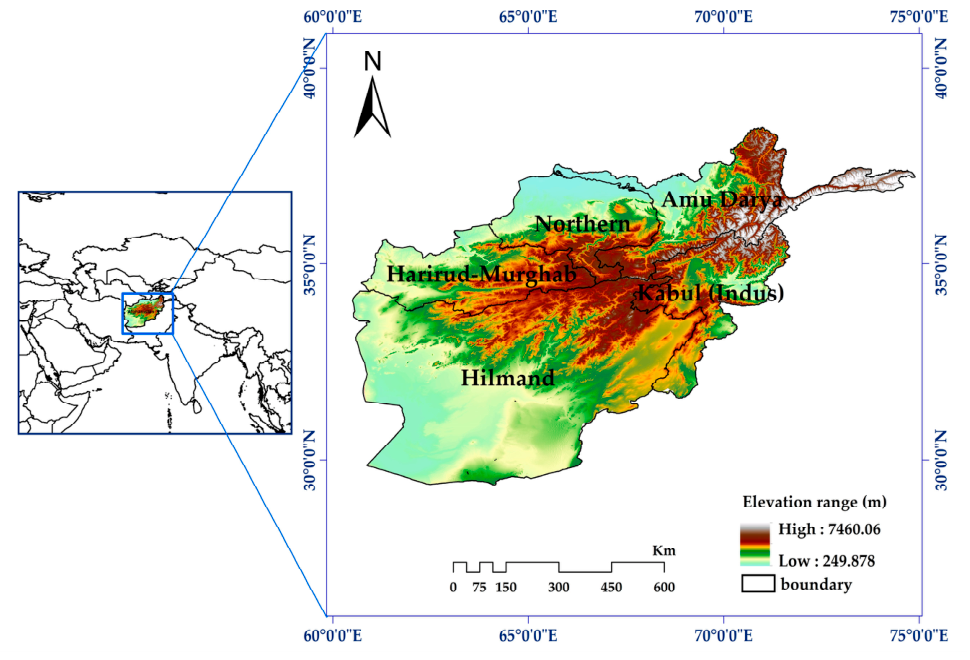
Figure 2.
LSTn trend (a), LSTn mean (b), NDVI trend (c), NDVI mean(d), SM trend (e), SM mean (f), PREC trend (g), and PREC mean (h).
Figure 2.
LSTn trend (a), LSTn mean (b), NDVI trend (c), NDVI mean(d), SM trend (e), SM mean (f), PREC trend (g), and PREC mean (h).
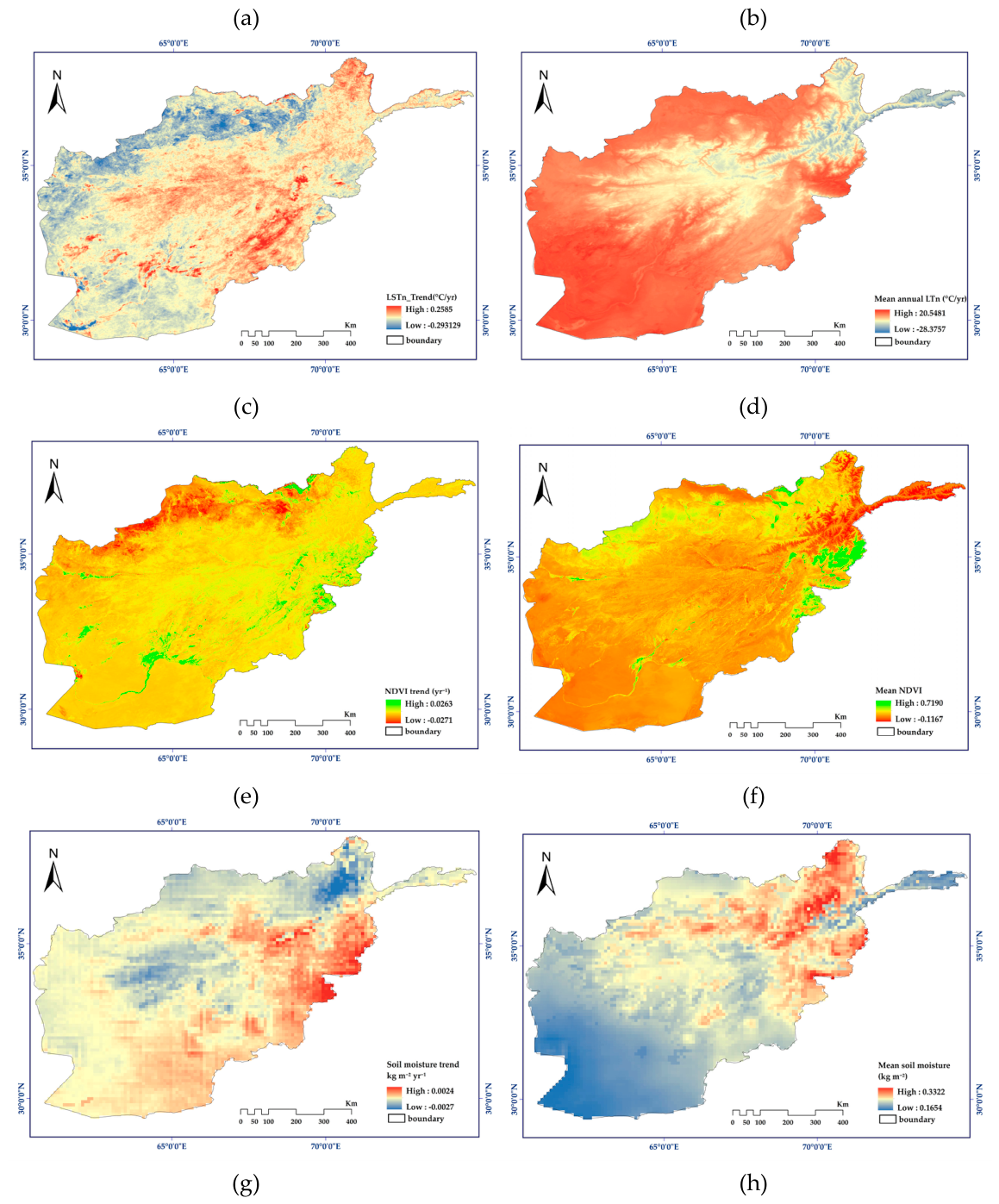
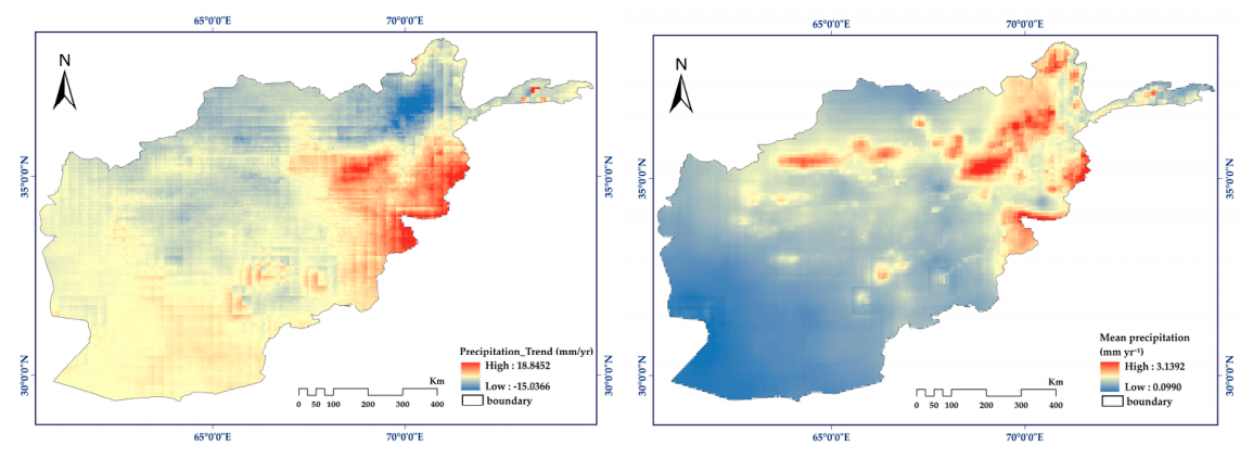
Figure 3.
The common nighttime LST forecasting framework processes.
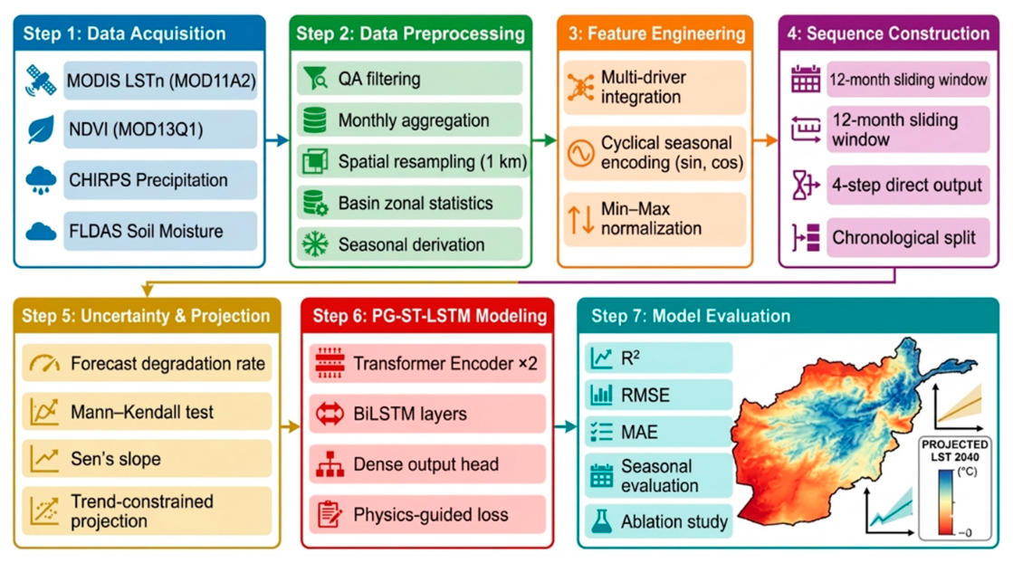
Figure 4.
The framework structure diagram
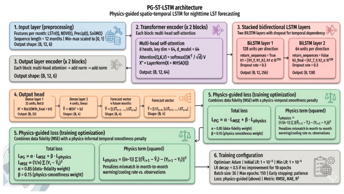
Figure 5.
LSTn Prediction (Historical-fit and Future prediction) using PG-ST-BiLSTM technique.
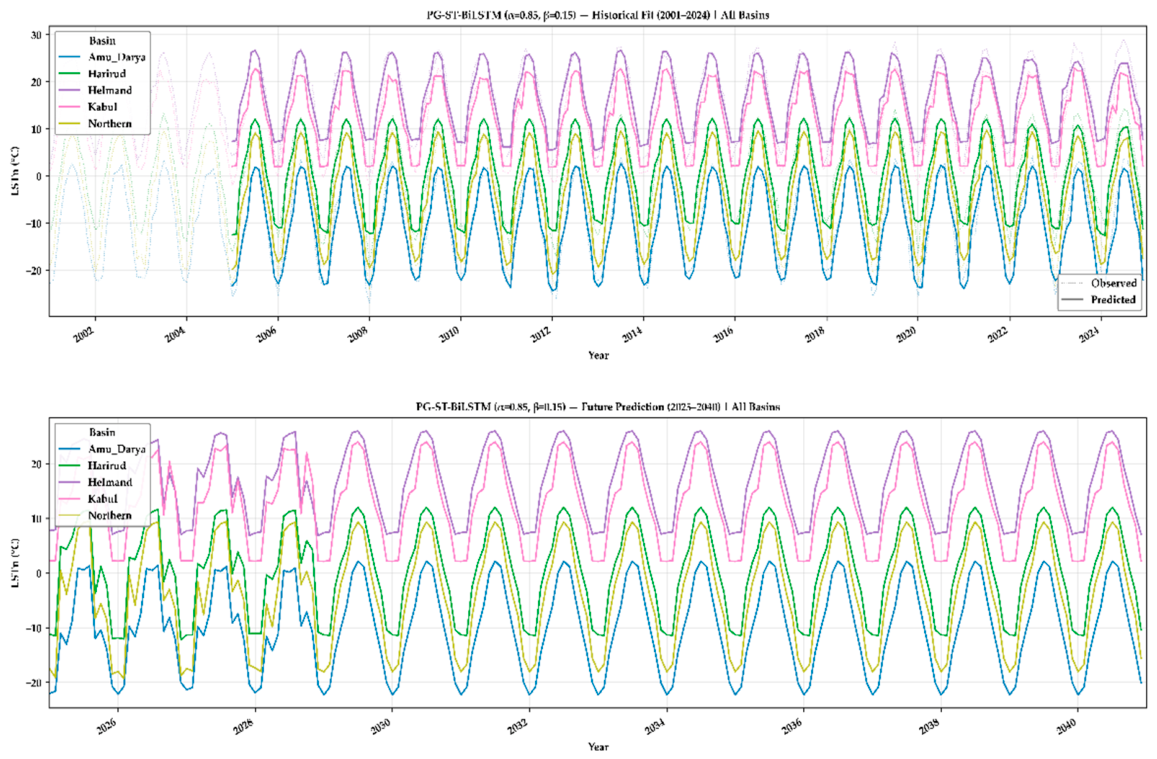
Figure 6.
Observed vs. fitted LSTn based on PG-ST-BiLSTM, LR, TCN, LSTM, and BiLSTM techniques.
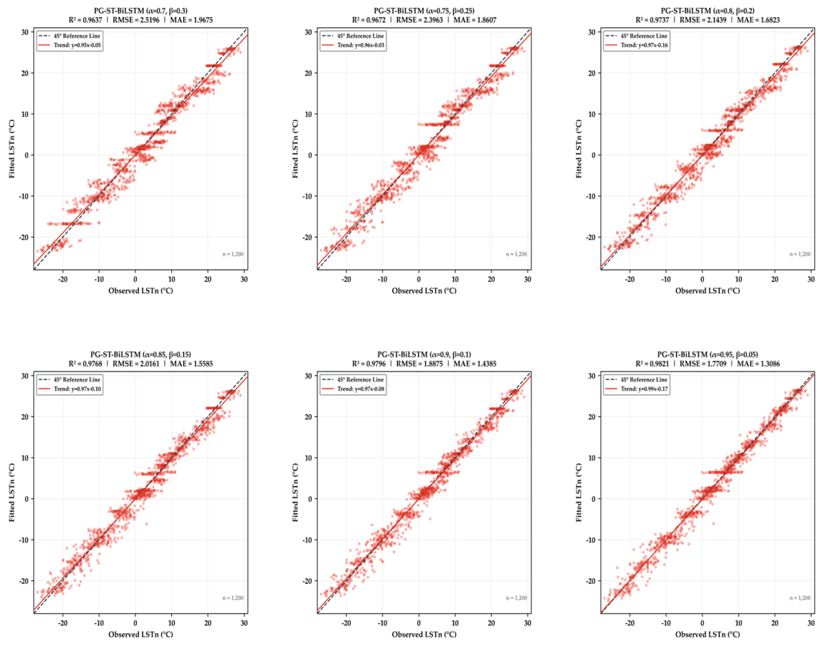
Figure 7.
Robustness Check of PG-ST-BiLSTM Under Loss Configuration (α=0.90, β=0.10).
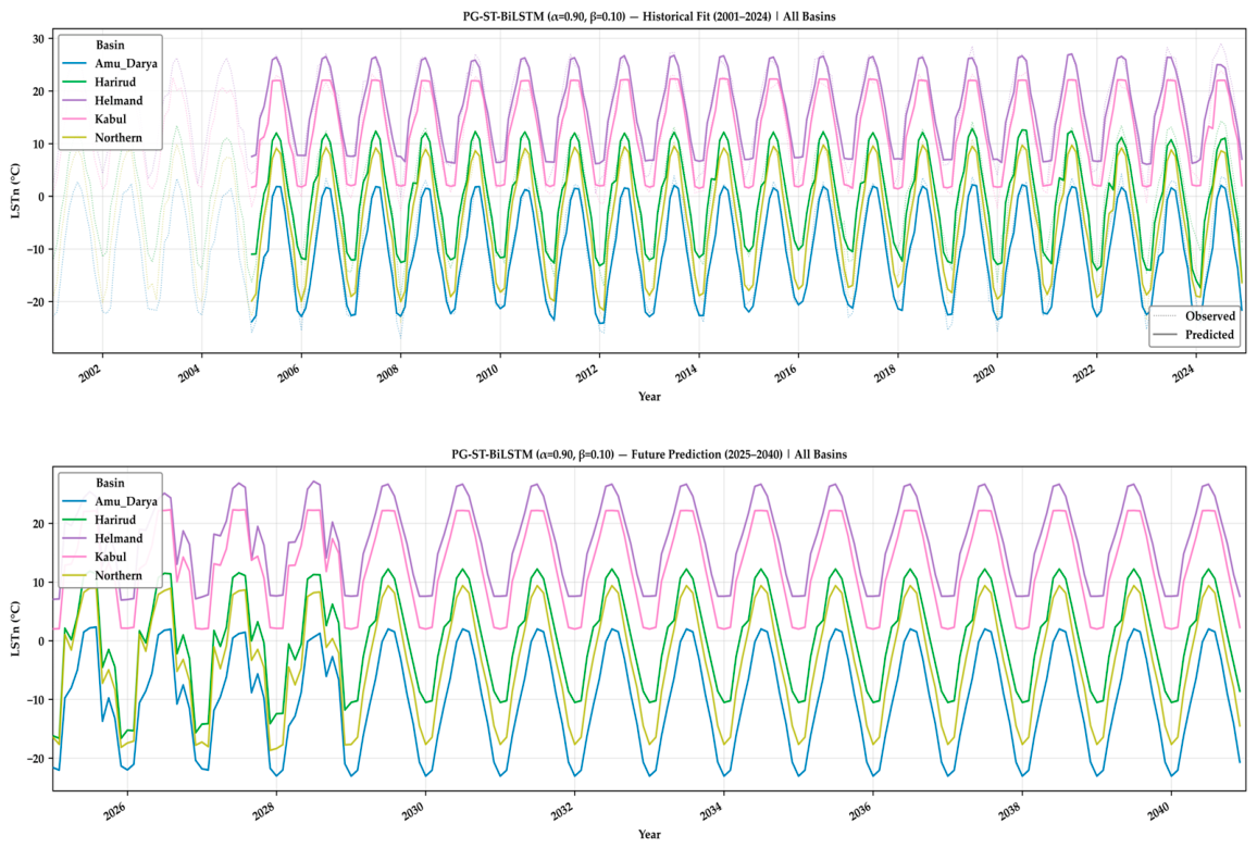

Table 1.
Summary of datasets used in this study.
| Data | Data type | T- Resolution | S-Resolution | Data source |
|---|---|---|---|---|
| LSTn | Raster | 8-day | 1 km | (MOD11A2), NASA Earth data (https://earthdata.nasa.gov/) |
| NDVI | Raster | 16-day | 250 m | (MOD13Q1), NASA Earth data (https://earthdata.nasa.gov/) |
| Precipitation | Raster | Daily | ~5.5 km | CHIRPS, Climate Hazards Center (https://chc.ucsb.edu/data/chirps) |
| Soil Moisture | Raster | Monthly | ~11 km | FLDAS NOAH01 V001, NASA GES DISC (https://disc.gsfc.nasa.gov/) |
Table 2.
Hyperparameter configuration for all forecasting models.
| Hyperparameter | PG-ST-BiLSTM | BiLSTM | LSTM | TCN | LR |
|---|---|---|---|---|---|
| Input window (months) | 12 | 12 | 12 | 12 | 12 |
| Prediction steps | 4 | 4 | 4 | 4 | 4 |
| Transformer blocks | 2 | — | — | — | — |
| Attention heads | 8 | — | — | — | — |
| Key dimension (d_k) | 64 | — | — | — | — |
| BiLSTM units (layer 1 / layer 2) | 64/32 | 64/32 | — | — | — |
| LSTM units (layer 1 / layer 2) | — | — | 64/32 | — | — |
| TCN filters / kernel size | — | — | — | 64/3 | — |
| TCN dilation rates | — | — | — | 1, 2, 4, 8 | — |
| Dropout rate | 0.3 | 0.3 | 0.3 | 0.3 | — |
| Dense layer units | 32 | 32 | 32 | 32 | — |
| Optimizer | Adam | Adam | Adam | Adam | OLS |
| Initial learning rate | 0.001 | 0.001 | 0.001 | 0.001 | — |
| LR decay factor | 0.5 (patience=5) | 0.5 | 0.5 | 0.5 | — |
| Early stopping patience | 15 epochs | 15 | 15 | 15 | — |
| Maximum epochs | 150 | 150 | 150 | 150 | — |
| Batch size | 32 | 32 | 32 | 32 | — |
| Loss function | LPG () | MSE | MSE | MSE | OLS |
| Total parameters | ~79,853 | ~41,220 | ~20,610 | ~18,432 | 4 |
Note: All DL models were implemented in TensorFlow 2.x and trained on identical data partitions (2001-2014 training; 2015-2024 validation) with identical preprocessing pipelines to ensure fair comparison.
Table 3.
Correlation Analysis by Season and Basin.
| Panel A: Correlation Analysis Based on Seasons. | |||||||||
| Variables | Winter | Spring | Summer | Autumn | |||||
| LSTn | LSTn | LSTn | LSTn | ||||||
| NDVI | 0.820 | 0.390 | -0.515 | -0.025 | |||||
| PREC | -0.362 | -0.633 | 0.173 | -0.494 | |||||
| SM | -0.014 | -0.580 | -0.040 | -0.451 | |||||
| Panel B: Correlation Analysis Based on Basins. | |||||||||
| Variables | Amu-Darya | Harirude | Helmand | Kabul | Northern | ||||
| LSTn | LSTn | LSTn | LSTn | LSTn | |||||
| NDVI | 0.811 | 0.837 | -0.065 | 0.155 | 0.899 | ||||
| PREC | -0.456 | -0.560 | -0.246 | -0.209 | -0.478 | ||||
| SM | -0.084 | -0.676 | -0.524 | -0.271 | -0.397 | ||||
Table 4.
The results of the multicollinearity analysis.
| Factors | Variance inflation factor | |
|---|---|---|
| VIF | 1/VIF | |
| PREC | 1.966 | .509 |
| SM | 1.837 | .544 |
| NDVI | 1.204 | .831 |
| Mean VIF | 1.669 | . |
Table 5.
Predictive performance comparison of PG-ST-BiLSTM and baseline models on the held-out validation set (2015-2024).
Table 5.
Predictive performance comparison of PG-ST-BiLSTM and baseline models on the held-out validation set (2015-2024).
| Rank | Model | R² | RMSE (°C) | MAE (°C) |
|---|---|---|---|---|
| 1 | PG-ST-BiLSTM (Proposed) | 0.977 | 2.023 | 1.534 |
| 2 | BiLSTM | 0.966 | 2.017 | 1.540 |
| 3 | LSTM | 0.966 | 2.426 | 1.975 |
| 4 | TCN | 0.961 | 2.426 | 1.971 |
| 5 | Linear Regression | 0.926 | 2.262 | 1.668 |
Table 6.
Mann-Kendall Sen’s Slope (°C/yr) of PG-ST-BiLSTM projected LSTn across seasons and basins (2025-2040).
Table 6.
Mann-Kendall Sen’s Slope (°C/yr) of PG-ST-BiLSTM projected LSTn across seasons and basins (2025-2040).
| Season | Northern | Kabul | Amu-Darya | Harirud | Helmand | Mean per season |
|---|---|---|---|---|---|---|
| Winter | 0.0185 | 0.0421 | 0.0110 | 0.0100 | 0.0358 | 0.1174 |
| Spring | 0.0111 | 0.0087 | 0.0091 | 0.0107 | 0.0108 | 0.0504 |
| Summer | 0.0118 | 0.0164 | 0.0246 | 0.0285 | 0.0171 | 0.0984 |
| Autumn | 0.0088 | 0.0104 | 0.0013 | 0.0181 | 0.0159 | 0.0545 |
| Mean per basin | 0.0502 | 0.0776 | 0.0460 | 0.0673 | 0.0796 | - |
| Mean per year | - | - | - | - | - | 0.0160 |
Disclaimer/Publisher’s Note: The statements, opinions and data contained in all publications are solely those of the individual author(s) and contributor(s) and not of MDPI and/or the editor(s). MDPI and/or the editor(s) disclaim responsibility for any injury to people or property resulting from any ideas, methods, instructions or products referred to in the content. |
© 2026 by the authors. Licensee MDPI, Basel, Switzerland. This article is an open access article distributed under the terms and conditions of the Creative Commons Attribution (CC BY) license (http://creativecommons.org/licenses/by/4.0/).
Copyright: This open access article is published under a Creative Commons CC BY 4.0 license, which permit the free download, distribution, and reuse, provided that the author and preprint are cited in any reuse.


