

Submitted:
27 June 2026
Posted:
29 June 2026
You are already at the latest version
Abstract
Search and rescue (SAR) for disaster response involves quick and efficient exploration of large, uncertain, and dangerous spaces. In this paper, we introduce a swarm-drone SAR approach with a key innovation in the form of directional pheromone gradient observation, where each agent’s RL policy is informed not only by local pheromone levels but also by the directional gradients in victim likelihood and coverage in four spatial cones, along with neighbor density information. These attributes are based on four virtual pheromone layers, each evolving independently and representing coverage history, victim likelihood, environment risk, and communication quality. The system uses a centralized training with decentralized execution (CTDE) MARL approach. Experiments were conducted on a custom-designed 40×40 grid-world environment involving 10 drones and 20 victims whose locations are unknown to all agents at episode start, with 180 static obstacles and 50 static hazard zones, over 5,000 training episodes and 30 independent evaluation runs. The hybrid agent achieved 98.9% area coverage and 93.3% victim detection, exceeding the RL-only baseline by 17.1 and 21.6 percentage points, respectively, across five independent training seeds (pooled n=150 evaluation runs). Welch’s t-test confirmed statistically significant improvements over RL-only for both area coverage (t=18.88, df=168, p<0.001, Cohen’s d=2.18) and victim detection (t=16.49, df=218, p<0.001, Cohen’s d=1.90). Ablation confirms that excluding directional gradient features reduces coverage and victim detection by 16.7 and 21.6 percentage points, respectively, identifying them as the dominant contributors to hybrid performance.
Keywords:
swarm drones
; edge AI
; search and rescue
; stigmergy
; reinforcement learning
; multi-agent reinforcement learning
; UAVs
; disaster response
; directional pheromone gradients
; decentralized coordination
1. Introduction
Natural and man-made catastrophes result in hazardous or impenetrable terrain for humans to conduct rescue missions. Quick localization of survivors is key, as research shows less than 50% of rescue probability within 24 hours after a structural collapse [1]. Unmanned aerial vehicles (UAVs) can swiftly deploy, capture thermal images, and enable communication despite broken ground-level facilities [2].
One drone alone would be incapable of handling a vast area due to battery limits, sensing range constraints, and the possibility of broken communication. Multiple drones can share tasks [3,4]; however, a fundamental question emerges in such an application scenario: how can many drones coordinate themselves effectively without having a delicate central controller when communication is broken?
This problem has been previously solved in one of two ways, namely, stigmergic principles [5], which enable indirect communication through leaving environmental traces similar to those of social insects, and multi-agent reinforcement learning (MARL) [6]. Stigmergy is efficient in communication costs but not adaptive since it requires fixed rules. MARL is capable of learning policies that can adapt to changing circumstances, yet is burdened by non-stationarity and sample inefficiency [7,8].
The critical idea presented by this paper is that by giving directional pheromone gradients as inputs to the RL observation, we can connect both worlds: stigmergy allows for the encoding of structured low-bandwidth coordination memory, whereas RL learns how to interpret and make use of this memory flexibly. Instead of considering the pheromone values as environmental variables, our design of the observation allows us to encode the direction of the victim information and unexplored areas.
The main research question is:How do directional pheromone gradient observations and neighbor density awareness improve decentralized MARL coordination for multi-drone SAR in uncertain disaster environments?.
The manuscript is organized as follows: Section 2 reviews related work. Section 3 presents the mathematical background. Section 4 describes the system and methodology. Section 5 reports results including ablation and communication loss experiments. Section 6 concludes.
The main contributions are:
- The decentralized multi-agent reinforcement learning pheromone gradient observation framework, where each drone observes pheromone fields indicating victim-likelihood and coverage. Agents do not need a global map, they coordinate their search/exploration according to the field patterns in the local area.
- A multiple-layer virtual pheromone model. These layers represent specific environmental factors, such as searched areas, possible victim locations, hazard zones, and communication quality. The layers cannot be maintained if they exist alone and provide a common environmental memory for the swarm without a centralized mapping. This is appropriate for the situation in CTDE (Training with richer information and decentralized execution).
- A hybrid stigmergy-MARL (indirect coordination from biological systems and reinforcement learning). Agents learn to improve their behavior using reward signals and simple low-bandwidth environmental cues, while several baselines are used to benchmark against, feature ablations are used to evaluate the framework, and communication failures are used to test it.
- The purpose of these experiments is to evaluate the effectiveness and robustness of the observation design under disaster search and rescue environment.
2. Literature Review
2.1. Swarm Robotics
In swarm robotics, the behavior of large numbers of simple robots is studied as a useful collective behavior, arising from local rules and decentralized interaction [9]. The field is inspired by swarm intelligence proposed by Beni and Wang [10].These systems are attractive because they’re easy to use: They scale, they’re resilient to failure, and they can handle several actions simultaneously. That last is more important than usual during disaster response. If one drone is down then the mission should not be stopped [11].
2.2. Execution and Swarm: Lightweight Models for Real-Time Autonomous Systems
In real swarm deployments, however, execution and swarm: Lightweight models for real-time autonomous systems coordination is just one of the issues. The models that operate on each agent must also be small and robust in the presence of noise and fast enough to track the environment. This is a common limitation in swarm robotics, autonomous vehicles, and distributed sensing, where agents typically don’t have a lot of compute and may not be able to wait.
Using demographic data, Shalash et al. [12] construct a multimodal deception detection system based on physiological signals, BPM, GSR and temperature. The accuracy of a Random Forest classifier optimized by Particle Swarm Optimization is 97% with an average inference time of 0.06 s, a significant improvement over those of the other classifiers, which demonstrates the ability of swarm-based optimization to produce fast and generalizable models even in sensitive detection tasks. Sallam et al. [13] on the other hand approach the Intelligent Dental Handpiece (IDH), a real-time dental skill assessment based on IMU. Both Logistic Regression and Random Forest achieved 100% accuracy at inference times under one millisecond, showing that lightweight ML is suitable for supporting precision-critical feedback for human-robot interaction.
In this work, Salah et al. [14] discuss another constraint, speaker verification in the context of an autonomous vehicle with stringent latency demands. Their Siamese network, which has both BiLSTM and Transformer encoders, achieves an EER of 0.0685 and an inference time of less than 0.2 s, a significant improvement over previous work. These three studies have something in common: in decentralized systems, it is not an option to have efficient model design, sensor fusion, or real-time execution. These are the minimum requirements.Shalash et al. [12] present an optimized polygraph-based deception detection system using multimodal physiological signals, including BPM, GSR, and temperature, together with demographic features. The data are processed with a Random Forest classifier that reaches 97% accuracy and 0.06 s inference latency. Particle Swarm Optimization (PSO) is used for hyperparameter tuning; it reduces the training-validation accuracy gap to under 1%. The authors also release a multimodal dataset collected from 49 participants. This work shows how swarm-inspired tuning can improve model generalization while keeping execution fast and resource-efficient, which is important in security and forensic applications where decisions must be quick and reliable.
Sallam et al. [13] introduce the Intelligent Dental Handpiece (IDH), an IMU-based motion analysis system for real-time skill assessment in dental training. The system classifies three motion states: Alert, Lever Range, and Stop Range. It uses features such as Deviation, Take Time, and Device type. Logistic Regression and Random Forest models both achieve 100% accuracy with sub-millisecond inference, allowing immediate visual and auditory feedback. The main point is direct: lightweight ML can support precision-critical human-machine interaction. This capability also transfers to swarm robotics, where individual agents need to carry out coordinated, sometimes dexterous actions with low latency.
Salah et al. [14] propose a lightweight speaker verification framework for autonomous vehicles. Their method combines Siamese networks with either BiLSTM or Transformer encoders, using triplet or quadruplet loss functions. On the LibriSpeech dataset, the best model, BiLSTM with triplet loss, achieves an equal error rate of 0.0685 and an inference time of 0.183 s, improving on prior work with an EER of 0.11. This highlights the need for efficient low-latency authentication in vehicular swarms, where secure identity verification must happen quickly to support personalized settings, command authentication, and driver monitoring without reducing safety or responsiveness.
Together, these studies show the same pattern. Scalable decentralized swarm intelligence needs efficient model design, sensor fusion, and real-time execution. Not as extra features, but as core requirements in dynamic environments.
2.3. Stigmergy and Virtual Pheromones
Stigmergy and Virtual Pheromones: Stigmergy is a type of coordination without direct communication between agents. Rather, they change a common environment, and other agents respond to the changes made [5,15]. The idea is based on social insects, bees and ants, in which no central authority is in charge of the group and it arises from simple local actions [16]. The agents leave a trace and the swarm reads this trace to make adjustments.
The most popular computational implementation of this idea is Ant Colony Optimization (ACO) [16].Useful paths and distributed route information develop over time as ants leave pheromones on them that will affect subsequent ants [17]. In swarm robotics, the idea is taken to a different level and the physical pheromone fields are replaced by virtual pheromone fields, which are stored, modified, and sensed by the robots digitally.
The virtual pheromone can be used in the search and rescue (SAR) application, where it can facilitate the decentralized control without requiring the ongoing communication among agents [18]. Agents can tag explored areas, probable victim locations, or unsafe locations, and other agents within that area can update their behaviors accordingly. However, the problem in the present SAR systems is that the majority of the existing ones follow a fixed rule and some of the primitive pheromone design. It reduces their adaptability, particularly in a mission that demands exploring, locating victims and avoiding the dangers in fluctuating environments.
2.4. Reinforcement Learning and MARL for Coverage
Reinforcement Learning has been providing autonomous agents with a means to learn decision-making by interacting with the environment [19]. Multi-agent reinforcement learning (MARL) extends this to multi-agent systems with multiple agents needing to learn to cooperate with each other in a partially observed environment with decentralized execution. The combination of that makes MARL suitable for UAV search, exploration and coverage as agents the operate in dynamic environments that are uncertain and partially visible.
A few studies have focused on directly addressing multi-UAV coordination using MARL. Pham et al. [7] presented a cooperative distributed RL approach for area-searching behavior in UAV field coverage, demonstrating that a set of multiple agents could learn coordinated area-searching behavior from local interaction without the need for centralized control. Later, MARVEL combined graph attention mechanisms into a MARL framework to enhance coordination for multi-robot environments with a large number of robots [8]. These works highlight the ability of MARL to learn complex cooperative behaviors without relying on handcrafted control policies.
The growing relevance of MARL for UAV coordination is reflected in recent surveys. Ekechi et al. identified MARL as a promising approach for UAV control in dynamic and uncertain environments [20], while Blais and Akhloufi reviewed advances in RL-based swarm robotics and emphasized the increasing role of learning-based coordination in multi-robot systems [21]. In disaster-response scenarios, Lee et al. investigated reinforcement learning for UAV-assisted emergency communication [22], and Tan and Zhao applied deep reinforcement learning to coordinate multiple UAVs for post-disaster search-and-rescue operations [1].
Despite these advances, most MARL-based approaches learn coordination solely from agent observations or explicit communication mechanisms. Relatively little attention has been given to incorporating structured environmental memory into the learning process. This is what leads to the need for agents to relearn useful coordination patterns through long training or rely on communication methods that may fail in disaster settings. This creates a clear need to combine stigmergic environmental cues with learned policies. Agents can then use shared information left in the environment while still keeping the flexibility of reinforcement learning.
2.5. Representation Learning in MARL
Representation Learning in MARL Methods for encoding observations directly influence coordination, their robustness and speed of convergence. Raw observations are sometimes not enough. Recent research in MARL has progressed towards the development of structured representations with spatial, temporal, or relational attributes, which enable agents to process partial observability, non-stationarity, and sparse exploration signals.
Hamdi et al. [23] introduce a multimodal attentional representation learning framework which integrates visual and temporal data. CNNs are used to extract features from the visual data, LSTMs to identify temporal patterns, and an attention mechanism to allow the model to concentrate on the most informative inputs. The multi-modality joint representation-based learning outperforms single-modality baselines, achieving up to 97% accuracy in classification and a 19%-57% boost in prediction performance. This finding is consistent with a larger hypothesis: when there are unclear or inconsistent observations, multimodal learning with attention is beneficial.
Li et al. [24] propose RACE that decouples the representation learning from policy learning in a MARL system. The agents are equipped with a shared observation encoder, while they have different policy representations, this means that transferring knowledge doesn’t result in the same behaviour being enforced. RACE deals with the challenges of partial observability by maximizing value-aware mutual information, thus learning features that contain globally relevant information. In several benchmark tasks, it achieves better coordination quality and convergence rate than baseline MARL approaches. The main point is clear: structured representations plus information-aware objectives can make multi-agent learning more effective.
Xu et al. [25] focus on multi-view representation learning, where data from several sources are fused into a more complete representation. Their Progressive Deep Multi-view Fusion (PDMF) method uses two stages. It consists of pre-training to capture relationships between views, then fine-tuning to map partial representations into complete ones. The model captures both consistency and complementarity across views which fixes some limits of standard fusion methods. Experiments on multiple datasets show steady gains over state-of-the-art approaches with classification accuracy improving by up to several percentage points. This supports the value of structured feature integration and progressive learning for better robustness and generalization.
Together, these studies show that stronger representation learning, through multimodal fusion, shared encoders, or multi-view integration, can improve learning efficiency, stability, and coordination in complex environments. For MARL, this supports the use of structured observation representations, where richer inputs can directly shape better policy performance.
2.6. Communication and Coordination in MARL
Communication and coordination are still hard problems in multi-agent reinforcement learning (MARL) especially when the system becomes larger, agents see only part of the environment and bandwidth is limited. Recent work has started to use learnable communication methods like dynamic coordination set selection, noise-aware communication and shared memory structures [26]. These methods do not treat communication as a fixed channel. Instead, they learn when agents should communicate, what information they should send, and how it should be shared.
Zhang and Lesser [27] propose a utility-based method helping agents find useful coordination sets during learning and reducing communication cost while keeping performance. Tung et al. [28] study learning-to-communicate over noisy physical channels where policies and channel coding are learned together rather than separately. Pesce and Montana [29] introduce a memory-based communication architecture that lets agents form emergent protocols for tasks that need close synchronization. Together, these works show a clear shift in MARL where agents coordinate better when communication and policy learning are designed jointly.
Zhang and Lesser [27] deal with scalability by allowing agents to find useful coordination sets while they learn. Their method uses an interaction measure to estimate how much performance may be lost if agents do not coordinate. Agents communicate only when coordination is important. This reduces overhead while keeping performance close to the full-communication setting. In sensor network target tracking the method reduces communication by more than 80% with only a small performance drop. This shows the trade-off between performance and bandwidth use.
Tung et al. [28] study communication under noisy physical channels. They formulate the problem as a MARL setting, where noisy channels are part of the environment dynamics rather than an external issue. Their MA-POMDP model moves beyond the common error-free communication assumption and learns cooperative policies together with robust channel coding. Experiments on binary symmetric, AWGN, and bursty noise channels show that joint learning performs better than separation-based methods. In joint channel coding, the learned schemes outperform Hamming codes by up to 3.70 dB in block error rate.
Pesce and Montana [29] propose MD-MADDPG which uses a shared memory device as a learnable communication channel under the centralized training and decentralized execution paradigm. Agents learn gated read and write operations so they can update and interpret memory while also learning their policies. Tested on six coordination-heavy navigation tasks, MD-MADDPG performs better than MADDPG and other baselines, mainly in synchronization tasks. The memory visualizations show task-related usage patterns, and the ablation results confirm that the main architectural components are needed.
2.7. UAVs in Disaster SAR
In SAR missions, UAVs are highly important since they enable fast exploration of hazardous, damaged, or difficult-to-reach areas without the danger to human lives of the searchers. According to recent literature, UAVs aid SAR operations with respect to rapid deployment, aerial surveillance, sensor-based victim identification, and operating in restricted areas [30].
The use of multiple UAVs enhances the performance of SAR tasks through the parallel exploration of various regions. Yet, several issues arise when employing multi-UAVs, including mission allocation, avoiding collisions, limited battery capacity, and poor communication in disaster zones. According to Ghauri et al. [31], the problem of dynamic mission allocation remains one of the critical issues for multiple UAVs conducting SAR activities.
2.8. Research Gap
Existing MARL approaches focus on learning coordination through policy optimization or explicit communication, while stigmergy-based systems rely on fixed rules without adaptability. However, little work explores structured, directional representations of environmental memory that can guide decentralized policies without communication overhead.
In particular, current approaches either depend on learned communication strategies, which introduce additional system complexity, or rely on static stigmergic rules that lack adaptability in dynamic environments. This creates a gap in developing methods that retain the efficiency of stigmergy while enabling adaptive, learned coordination.
These particular gaps prompt this research in three ways. First, Salman et al. [18] perform automated stigmergy behavior design yet lack the learning mechanism whereby their system cannot prioritize adaptively. Second, Tan and Zhao [1] implement a deep RL strategy for multiple UAVs in SAR tasks using a centralized approach that falls short when the base station gets compromised. Third, Pham et al. [7] and MARVEL [8] illustrate the use of reinforcement learning techniques in multi-robot task accomplishment while excluding the use of pheromones to communicate past actions. This means that the robots have to learn how to coordinate with each other based solely on observation. To the best of our knowledge, this is among the first SAR awareness under a CTDE-based MARL setting.
3. Methodology
The methodology is designed to isolate the impact of directional pheromone gradient observations on decentralized coordination performance, ensuring that all other components of the system remain consistent across compared approaches.
3.1. Problem Formulation and Environment
Disaster search and rescue (SAR) operations are inherently stochastic and partially observable. The locations of victims are not known, there may be obstacles in the way, and communication between agents may be faulty. Hence, the problem is formulated as a Decentralized Partially Observable Markov Decision Process (Dec-POMDP), where each UAV makes decisions based on its own local observations.
The disaster site is modeled by a grid G, with each square possibly being free, obstructed, dangerous, searched, or occupied by a victim. At each time step t, UAV i has a local observation , current location , current battery life , and an action . Each agent can see within its own local window, with sensing range .
The environment is generated procedurally using a fixed random seed per episode. Obstacles, hazard zones, and victim locations are sampled uniformly at random without replacement from all grid cells outside a central exclusion zone reserved for drone initialisation. Obstacles are impassable; hazard zones are traversable but penalise entry (reward ) and deposit risk pheromone . Both are static for the duration of each episode — neither obstacles nor hazard zones move. Victims are likewise stationary; their locations are unknown to agents until physically detected within sensing range (). The drones are uniformly randomized in the central square. No two drones occupy the same grid point in the starting position. Each of the 30 iterations uses a distinct map so that the performance on different maps can be measured. The entire source code of the simulation is provided along with this paper.
3.2. System Architecture
The proposed system has five layers, shown in Figure 1. The sensing layer collects RGB, thermal, LiDAR, IMU, and communication-signal data. The mapping layer builds local occupancy grids and victim-probability grids, then merges them across drones when communication is available. The stigmergy layer maintains and spreads the four pheromone maps using Equation (1). The learning layer runs the MARL policy. An optional mission-control layer tracks global progress and assigns area priorities. When it is disconnected, the system still runs in a fully decentralized way.
The proposed observation formulation is independent of the specific environment structure and can be applied to any decentralized MARL setting where spatial information is represented through local maps or distributed environmental fields.
3.3. Virtual Pheromone Model
To support indirect coordination, the proposed system uses four virtual pheromone layers inspired by stigmergy. The coverage layer marks scanned cells, the victim-likelihood layer stores possible human-presence evidence, the risk layer marks hazardous regions, and the communication layer identifies useful relay areas.
Each pheromone layer is updated through evaporation, diffusion, and new deposits:
where , is the evaporation rate, is the diffusion coefficient, is the four-cell neighborhood, and is the new deposited pheromone. The victim-likelihood layer uses the slowest evaporation rate, , so possible victim evidence remains available for longer.
3.4. Directional Pheromone Gradient Observation
The central design contribution is an enriched observation vector. Each drone i observes:
where is the directional victim-pheromone gradient. It is computed as the mean over a 3-cell cone in each cardinal direction. The term is computed in the same way, but for the coverage pheromone. gives the normalized number of drones within , while are binary obstacle indicators for the four directions. Neighbor density is taken from physical drone positions, so it gives short-range proximity awareness without active message exchange. It remains available even when communication is lost.
This directional representation reduces decision ambiguity. With only scalar pheromone values at the current cell, a drone knows what is happening where it stands, but not where the useful signal is stronger. It leads to inefficient exploration or back and forth moves under partial observability conditions. Representation by directional trends and provides a straightforward hint to the policy about where more victims’ signs are observed or, alternatively, where there is less coverage. In such a way, drones can explore more purposefully without the need for a global map or additional communication.
The detection of a victim takes place based on a deterministic binary scheme. The presence of a victim at the grid cell is determined if the drone visits any cell , for which . This means that the victim is located within a drone’s sensing window, where . Upon detection, the value of is added to the drone’s current position, and the victim is considered to be discovered. Positions of victims are unknown to all agents in the beginning of each episode. They are not included in the initial state or observation. The model abstracts a short-range thermal or visual sensor. A probabilistic detection model with distance-based false alarms is left for future work.
Overall, the added directional features make the observation more informative than scalar pheromone inputs alone. They let each agent infer local spatial gradients of coverage and victim likelihood, reduce ambiguity in action selection, and support more stable navigation in partially observable environments.
These features add more than scalar pheromone values alone. If a drone only observes at its current cell, it knows there is some victim-related signal nearby, but not where that signal is coming from. With , it can move toward the strongest victim-likelihood direction without needing a global map or explicit message passing.
Unlike conventional methods based only on scalar local observations the proposed representation encodes directional trends. This lets each agent infer spatial gradients of relevant environmental signals, reduces ambiguity in action selection and supports more purposeful navigation under partial observability.
Similarly, encodes which direction has the least explored space, enabling learned dispersion without inter-agent negotiation. The neighbor density allows the policy to avoid redundant clustering even when no explicit task-assignment protocol exists. An ablation study in Section V quantifies the individual contribution of each feature.
The proposed directional features introduce minimal computational overhead, as gradient values are computed from local pheromone maps using simple averaging operations over small spatial neighborhoods. A comparison between conventional scalar observations and the proposed directional representation is summarized in Table 1.
3.5. Hybrid Decision Process
Algorithm 1 formalizes the per-step procedure.
| Algorithm 1 Hybrid Stigmergy-RL Step (drone i, step t) |
|
3.6. Non-Learned Baselines
Three non-learned baselines are included for comparison. Random walk selects actions uniformly at random each step. Frontier search directs each drone to the nearest unvisited cell using Manhattan distance, with random tie-breaking. Stigmergy-only uses fixed hand-coded rules based solely on the shared pheromone field, with no learning: at each step, each drone scores the four cardinal moves using the linear combination , where , , are the pheromone values at the candidate cell and penalises cells occupied by other drones. A small uniform noise term breaks ties. The drone moves to the highest-scoring valid cell, or hovers if all moves are blocked. This rule prioritises victim-likelihood signals over coverage and avoids hazards and crowding — but the weights are fixed and cannot be adapted at runtime.
3.7. Training Strategy
Victim detection and cell creation are rewarded positively; energy consumption, collision, and entry into the danger zone are penalized. The victim coefficient takes precedence over all others, guaranteeing that the drone algorithm favors victim detection above cell creation. The communication reward ensures that the drones will stay in relay formation when no other high-priority task is available.
Tabular Q-learning is chosen deliberately for these experiments. It allows complete control of the observation space and makes it possible to separate the contribution of the suggested representation. It also helps avoid additional sources of noise caused by function approximation, making performance improvements associated solely with directional gradient representations easier to attribute.
The training regime adheres to the CTDE setup. During the training the simulator generates the global state used to calculate the reward, while during evaluation each drone selects actions based only on its individual observation. The Q-tables have a 6-bin quantization for each pheromone-relevant observation feature and are initialized in an optimistic way () to promote exploration early in the training process. To avoid conflict with the victim reward weight in Equation (3) the Q-learning step size is written as in Table 2. Exploration uses multiplicative decay, , applied once per episode with a minimum value of 0.05. Across 5,000 training episodes, drops from 1.0 to about 0.135 so exploration does not vanish. Each learned method is trained with five independent random seeds and results are reported as mean ± std across seeds to separate training-seed variance from evaluation variance. Statistical significance is tested using Welch’s t-test on pooled evaluation runs () along with Cohen’s d effect size and bootstrap 95% confidence intervals. For a fair comparison all models use the same reward function, training process and environment conditions. However, only the observation representation changes.
The RL-only baseline uses the same learning rate, discount factor, exploration schedule, training length and evaluation protocol as the hybrid model. It differs only in the observation or policy state. Table 3 gives the exact features for each model. Both models share five base features: local coverage pheromone with 6 bins, local victim pheromone with 6 bins, a binary risk flag from , normalized battery with 4 bins and four binary obstacle indicators. The hybrid model adds three more features: victim-gradient direction , defined as the dominant cardinal direction of ; coverage-gradient direction , defined as the direction of least-explored space; and neighbor density with 3 bins. The reported improvements are therefore attributable solely to these three added observation features. The RL-only baseline is intentionally matched to the hybrid in architecture, reward function, and training procedure, differing only in observation features (Table 3), so that any performance difference is attributable to the three added gradient features rather than to architectural differences.
The state space increases from 9 to 18 dimensions; however, due to discretization, the resulting Q-table remains computationally tractable within the evaluated environment size.
4. Results and Discussion
4.1. Training Convergence
Figure 2 shows the training reward smoothed with a 100-episode uniform moving average over 5,000 episodes. The hybrid model shows faster and more stable reward improvement than the RL-only baseline, indicating that directional pheromone-gradient observations provide useful structure for learning coordinated search behavior. This supports the role of pheromone-guided observations in reducing sample complexity compared with learning from local state features alone.
Not only achieving better performance at the end but this hybrid approach also converges much faster. Looking at the learning curve we see that it reaches stable behavior sooner compared to the RL-only baseline which implies that the knowledge of directional gradients helps the agent learn more efficiently.
4.2. Coverage and Victim Detection
Figure 3 depicts area coverage over time for all five approaches in 30 trials with confidence intervals. Evaluation results are given in Table 4. Hybrid agent achieves 98.9% area coverage and 93.3% victim detection, outperforming the pure RL approach by 17.1 pp and 21.6 pp respectively. Welch’s t-test shows that these gains are significant for both coverage (, , , Cohen’s ) and victim detection (, , , Cohen’s ). In addition, the coverage variance reduces from with RL-only approach to with the hybrid one indicating increased stability in decentralized execution due to observations of pheromone gradients.
4.3. Comparative Analysis
Benchmark results are shown in Figure 4. Hybrid algorithm provides 98.9% coverage and 93.3% victims detection greatly outperforming RL-based only algorithm providing 81.8% coverage and 71.7% victim detection. This is equivalent to gains of 17.1 percentage points in coverage and 21.6 percentage points in victims detection.
Stigmergy-only approach is also quite good achieving 86.5% coverage and 77.7% victims detection. Its fixed exhaustive exploration rules help it achieve better coverage than both random walk and RL-only, although it still remains below the hybrid model overall. However, unlike the learned hybrid model, it cannot adapt its behavior at runtime and therefore cannot flexibly prioritize changing mission objectives, energy constraints, or hazard conditions. The hybrid method outperforms stigmergy-only by 12.4 pp in coverage and 15.6 pp in victim detection while maintaining a fully learned, adaptive policy.
4.4. Ablation Study
To quantify the contribution of each proposed feature, we train and evaluate three variants: the full hybrid model, an ablated model without directional gradients (, removed), and an ablated model without neighbor density ( removed). Results are shown in Figure 5 and Table 5.
Removing directional gradients reduces coverage by 16.7 pp (98.9% → 82.3%) and victim detection by 21.6 pp (93.3% → 71.7%). This confirms that directional victim-likelihood and coverage gradients are the dominant contributors to the hybrid model’s performance. Excluding neighbor density reduces coverage by 0.2 pp (from 98.9% to 99.2%) and victim detection by 1.0 pp (from 93.3% to 94.3%), suggesting that neighbor density awareness plays a role in performance, though is less important than gradient information.
4.5. Robustness Under Communication Loss
To evaluate robustness under realistic degraded-communication conditions, each drone maintains its own local pheromone map during evaluation, merging (element-wise maximum) with neighbours whose link is currently up. Both models were evaluated across a sweep of communication-link failure probabilities: 0%, 25%, 50%, 75%, and 100%. At each level, each active pairwise link is severed independently with the given probability, preventing map merging between the affected drones and forcing each to rely solely on its own locally accumulated pheromone evidence. Note that is computed from physical drone positions rather than message exchange, and therefore remains available at all dropout levels; only pheromone-map sharing is gated by the dropout probability. Results are shown in Figure 6 and Table 6.
The hybrid model demonstrates strong robustness across the full sweep: coverage remains at 99.1% even at 100% link failure, a degradation of only 0.2 pp from the fully-connected baseline (99.3%). The RL-only agent similarly maintains stable performance, with both models relying on locally available pheromone information and learned policies that do not require active inter-agent coordination to function effectively. The hybrid model keeps a consistent –15 pp coverage lead over RL-only at every dropout level. This suggests that pheromone-based stigmergy gives a structural coordination advantage, and that advantage remains even when communication is fully lost.
4.6. Limitations
Four limitations are acknowledged. First, pheromone parameters (, ) require per-layer tuning; misspecification may cause premature forgetting of victim evidence or persistent misleading traces. Adaptive online tuning via meta-learning is a natural extension. Second, the sim-to-real gap, GPS denial, sensor noise, aerodynamic disturbances, irregular 3D terrain, must be addressed before physical deployment; AirSim or Webots validation is the recommended next step. Third, tabular Q-learning may underperform deep function approximators (QMIX, MAPPO) on larger or more complex environments, and the absolute performance ceiling of both the hybrid and RL-only models is therefore lower than what deep MARL would achieve on this task. The RL-only baseline is intentionally matched in architecture to the hybrid to isolate the contribution of the directional gradient observation features; comparison against deep MARL baselines (QMIX, MAPPO, independent DQN) is deferred to future work. Fourth, safety-critical outdoor UAV operations require geofencing, fail-safe landing protocols, and regulatory compliance beyond the scope of this work. Fifth, while the communication-dropout sweep implements per-drone local pheromone maps with independent link failures, it does not model message delays, partial map corruption, or time-varying link quality. These represent important aspects of realistic disaster communication channels and are acknowledged as a current limitation of the robustness evaluation.
Additionally, the proposed representation is evaluated within a discretized state space using tabular reinforcement learning. While this setup allows controlled evaluation of the representation itself, further validation with deep function approximators and continuous observation spaces is required to assess scalability in more complex environments.
5. Conclusions
This paper introduced a directional pheromone gradient observation for decentralized swarm-drone disaster SAR combining stigmergy and MARL. The key insight is that feeding directional gradients of victim likelihood and coverage, rather than scalar local values, into the RL policy enables purposeful navigation toward victim evidence and unexplored regions without global map access or explicit inter-agent negotiation. Four independently parameterized pheromone layers provide evaporating shared memory that serves as a structured coordination substrate under the CTDE paradigm.
Experiments over 5,000 training episodes and 30 independent evaluation runs on a grid demonstrate that the hybrid model achieved 98.9% coverage and 93.3% victim detection. Compared with the RL-only baseline the hybrid model improves coverage by 17.1 pp and victim detection by 21.6 pp. The differences are statistically significant for both coverage (, , , Cohen’s ) and victim detection (, , , Cohen’s ). A similar conclusion can be reached from the ablative experiment where removal of the directional gradient leads to a coverage decrease of 16.7 pp and detection decrease of 21.6 pp. Communication-dropout experiments in the range from 0 to 100% link failures demonstrate that the hybrid solution preserves at least 99% coverage on all stages with consistent 14–15 pp gain over RL-only.
The future works are aimed at shifting away from the tabular Q learning to advanced techniques such as QMIX and MAPPO, along with neural pheromone encoders for continuous state spaces and large maps. Adaptive meta-learning of per-layer evaporation coefficients will be implemented to reduce the number of hyperparameters. The scalability analysis will be performed up to grid maps with up to 50 drones. More complex communication experiments will be carried out using time-varying dropouts, delayed messages, and partial map destruction rather than simple link-failure scenarios considered in this study. Physical validation via AirSim or Webots simulations along with field experiments will be useful for reducing the sim-to-real gap before deployment. The directional gradient observation is architecture-agnostic and directly transferable to any MARL framework receiving environmental map features.
Author Contributions
Conceptualization, P.Y., M.M.K. and O.S.; methodology, P.Y., M.M.K. and O.S.; software, P.Y. and M.M.K.; validation, P.Y., M.M.K. and O.S.; formal analysis, P.Y. and M.M.K.; investigation, P.Y. and M.M.K.; resources, O.S.; data curation, P.Y. and M.M.K.; writing—original draft preparation, P.Y. and M.M.K.; writing—review and editing, P.Y., M.M.K., E.K. and O.S.; visualization, P.Y. and M.M.K.; supervision, O.S.; project administration, O.S. All authors have read and agreed to the published version of the manuscript.
Funding
This research received no external funding.
Institutional Review Board Statement
Not applicable.
Informed Consent Statement
Not applicable.
Data Availability Statement
The simulation code and supporting material are available in the supplementary material.
Acknowledgments
The researchers acknowledge Ajman University for its support in this research.
Conflicts of Interest
The authors declare no conflicts of interest.
Abbreviations
The following abbreviations are used in this manuscript:
| ACO | Ant Colony Optimization |
| CTDE | Centralized Training with Decentralized Execution |
| Dec-POMDP | Decentralized Partially Observable Markov Decision Process |
| GPS | Global Positioning System |
| IMU | Inertial Measurement Unit |
| LiDAR | Light Detection and Ranging |
| MARL | Multi-Agent Reinforcement Learning |
| Q-learning | Value-based reinforcement learning algorithm using action-value functions |
| RGB | Red–Green–Blue |
| RL | Reinforcement Learning |
| SAR | Search and Rescue |
| UAV | Unmanned Aerial Vehicle |
References
- Tan, L.; Zhao, H. A Multi-UAV Rapid Post-Disaster Search and Rescue Method Based on Deep Reinforcement Learning. Complex Intell. Syst. 2026, 12, 41. [Google Scholar] [CrossRef]
- Said, H.; Mahar, K.; Sorour, S.E.; Elsheshai, A.; Shaaban, R.; Hesham, M.; Khadr, M.; Mehanna, Y.A.; Basha, A.; Maghraby, F.A. IMITASD: Imitation Assessment Model for Children with Autism Based on Human Pose Estimation. Mathematics 2024, 12, 3438. [Google Scholar] [CrossRef]
- Yasser, M.; Shalash, O.; Ismail, O. Optimized Decentralized Swarm Communication Algorithms for Efficient Task Allocation and Power Consumption in Swarm Robotics. Robotics 2024, 13, 66. [Google Scholar] [CrossRef]
- Said, H.; Akbari, A.S.; Moniri, M. An adaptive reference frame re-ordering algorithm for H. 264/AVC based multi-view video codec. In Proceedings of the 21st European Signal Processing Conference (EUSIPCO 2013); IEEE, 2013; pp. 1–5. [Google Scholar]
- Theraulaz, G.; Bonabeau, E. A Brief History of Stigmergy. Artif. Life 1999, 5, 97–116. [Google Scholar] [CrossRef] [PubMed]
- Zhang, K.; Yang, Z.; Başar, T. Multi-agent reinforcement learning: A selective overview of theories and algorithms. Handb. Reinf. Learn. Control 2021, 321–384. [Google Scholar] [CrossRef]
- Pham, H.X.; La, H.M.; Feil-Seifer, D.; Nefian, A. Cooperative and Distributed Reinforcement Learning of Drones for Field Coverage. arXiv 2018, arXiv:1803.07250. [Google Scholar]
- Cao, M.; et al. MARVEL: Multi-Agent Reinforcement Learning for Constrained Field-of-View Multi-Robot Exploration in Large-Scale Environments. arXiv 2025, arXiv:2502.20217. [Google Scholar]
- Sahin, E. Swarm Robotics: From Sources of Inspiration to Domains of Application. Lecture Notes in Computer Science; In Swarm Robotics; Springer, 2005; Vol. 3342, pp. 10–20. [Google Scholar]
- Beni, G.; Wang, J. Swarm Intelligence in Cellular Robotic Systems. In Robots and Biological Systems: Towards a New Bionics? Springer, 1993; pp. 703–712. [Google Scholar]
- Fawzy, H.; Elbrawy, A.; Amr, M.; Eltanekhy, O.; Khatab, E.; Shalash, O. A systematic review: Computer vision algorithms in drone surveillance. J. Robot. Integr. 2025, 2, 1–10. [Google Scholar]
- Shalash, O.; Metwalli, A.; Sallam, M.; Khatab, E. A Multimodal Polygraph Framework with Optimized Machine Learning for Robust Deception Detection. Inventions 2025, 10, 96. [Google Scholar] [CrossRef]
- Sallam, M.; Salah, Y.; Osman, Y.; Hegazy, A.; Khatab, E.; Shalash, O. Intelligent Dental Handpiece: Real-Time Motion Analysis for Skill Development. Sensors 2025, 25, 6489. [Google Scholar] [CrossRef] [PubMed]
- Salah, Y.; Shalash, O.; Khatab, E. A Lightweight Speaker Verification Approach for Autonomous Vehicles. J. Robot. Integr. Manuf. Control 2024, 1–16. [Google Scholar]
- Heylighen, F. Stigmergy as a Universal Coordination Mechanism I: Definition and Components. Cogn. Syst. Res. 2016, 38, 4–13. [Google Scholar] [CrossRef]
- Dorigo, M.; Birattari, M.; Stutzle, T. Ant Colony Optimization: Artificial Ants as a Computational Intelligence Technique. IEEE Comput. Intell. Mag. 2006, 1, 28–39. [Google Scholar] [CrossRef]
- Métwalli, A.; Fathy, F.; Khatab, E.; Shalash, O. ER-ACO: A Real-Time Ant Colony Optimization Framework for Emergency Medical Services Routing and Hospital Resource Scheduling. Algorithms 2026, 19, 102. [Google Scholar] [CrossRef]
- Salman, M.; Ramos, D.G.; Birattari, M. Automatic Design of Stigmergy-Based Behaviours for Robot Swarms. Commun. Eng. 2024, 3, 30. [Google Scholar] [CrossRef]
- Sutton, R.S.; Barto, A.G. Reinforcement Learning: An Introduction, 2 ed.; MIT Press, 2018. [Google Scholar]
- Ekechi, C.C.; Elfouly, T.; Alouani, A.; Khattab, T. A Survey on UAV Control with Multi-Agent Reinforcement Learning. Drones 2025, 9, 484. [Google Scholar] [CrossRef]
- Blais, M.A.; Akhloufi, M.A. Reinforcement Learning for Swarm Robotics: An Overview. Cogn. Robot. 2023, 3, 226–256. [Google Scholar] [CrossRef]
- Lee, I.; Babu, V.; Caesar, M.; Nicol, D. Deep Reinforcement Learning for UAV-Assisted Emergency Response. In Proceedings of the Proceedings of the 17th EAI International Conference on Mobile and Ubiquitous Systems: Computing, Networking and Services (MobiQuitous), 2020; pp. 174–183. [Google Scholar]
- Hamdi, A.; Aboeleneen, A.; Shaban, K. MARL: Multimodal Attentional Representation Learning for Disease Prediction. Proc. Int. Conf. Comput. Vis. Syst. (ICVS) Lecture Notes in Computer Science. 2021, Vol. 12899, 14–27. [Google Scholar] [CrossRef]
- Li, P.; Hao, J.; Tang, H.; Zheng, Y.; Fu, X. RACE: Representation Asymmetry and Collaborative Evolution for Multi-Agent Reinforcement Learning. In Proceedings of the Proceedings of the International Conference on Machine Learning (ICML), 2023. [Google Scholar]
- Xu, C.; Zhao, W.; Zhao, J.; Guan, Z.; Yang, Y.; Chen, L.; Song, X. Progressive Deep Multi-View Comprehensive Representation Learning. In Proceedings of the Proceedings of the AAAI Conference on Artificial Intelligence, 2023. [Google Scholar]
- Chafii, M.; Naoumi, S.; Alami, R.; Almazrouei, E.; Bennis, M.; Debbah, M. Emergent Communication in Multi-Agent Reinforcement Learning for Future Wireless Networks. IEEE Internet Things Mag. 2023, 6, 18–24. [Google Scholar] [CrossRef]
- Zhang, C.; Lesser, V. Coordinated Multi-Agent Reinforcement Learning with Controlled Communication. In Proceedings of the Proceedings of the 10th International Conference on Autonomous Agents and Multiagent Systems (AAMAS), IFAAMAS, 2011; pp. 1101–1108. [Google Scholar]
- Tung, T.Y.; Kobus, S.; Roig, J.P.; Gündüz, D. Effective Communications: A Joint Learning and Communication Framework for Multi-Agent Reinforcement Learning Over Noisy Channels. IEEE J. Sel. Areas Commun. 2021, 39, 2590–2603. [Google Scholar] [CrossRef]
- Pesce, E.; Montana, G. Improving Coordination in Small-Scale Multi-Agent Deep Reinforcement Learning Through Memory-Driven Communication. Mach. Learn. 2020, 109, 1727–1747. [Google Scholar]
- Quero, C.O.; Martinez-Carranza, J. Unmanned Aerial Systems in Search and Rescue: A Global Perspective on Current Challenges and Future Applications. Int. J. Disaster Risk Reduct. 2025, 118, 105199. [Google Scholar] [CrossRef]
- Ghauri, S.A.; Sarfraz, M.; Qamar, R.A.; Sohail, M.F.; Khan, S.A. A Review of Multi-UAV Task Allocation Algorithms for a Search and Rescue Scenario. J. Sens. Actuator Netw. 2024, 13, 47. [Google Scholar] [CrossRef]
Figure 1.
Five-layer hybrid stigmergy-RL architecture. The dashed arrow shows pheromone deposits fed back from the learning layer. The learning layer receives directional gradients , computed from the stigmergy layer, not just local scalar values.
Figure 1.
Five-layer hybrid stigmergy-RL architecture. The dashed arrow shows pheromone deposits fed back from the learning layer. The learning layer receives directional gradients , computed from the stigmergy layer, not just local scalar values.
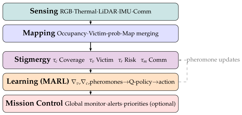
Figure 2.
Training reward smoothed with a 100-episode uniform moving average (window = 5,000/50) over 5,000 episodes, mean across 5 seeds. The hybrid model performs better than the RL-only approach, showing that pheromone-gradient cues make learning faster and more effective.
Figure 2.
Training reward smoothed with a 100-episode uniform moving average (window = 5,000/50) over 5,000 episodes, mean across 5 seeds. The hybrid model performs better than the RL-only approach, showing that pheromone-gradient cues make learning faster and more effective.
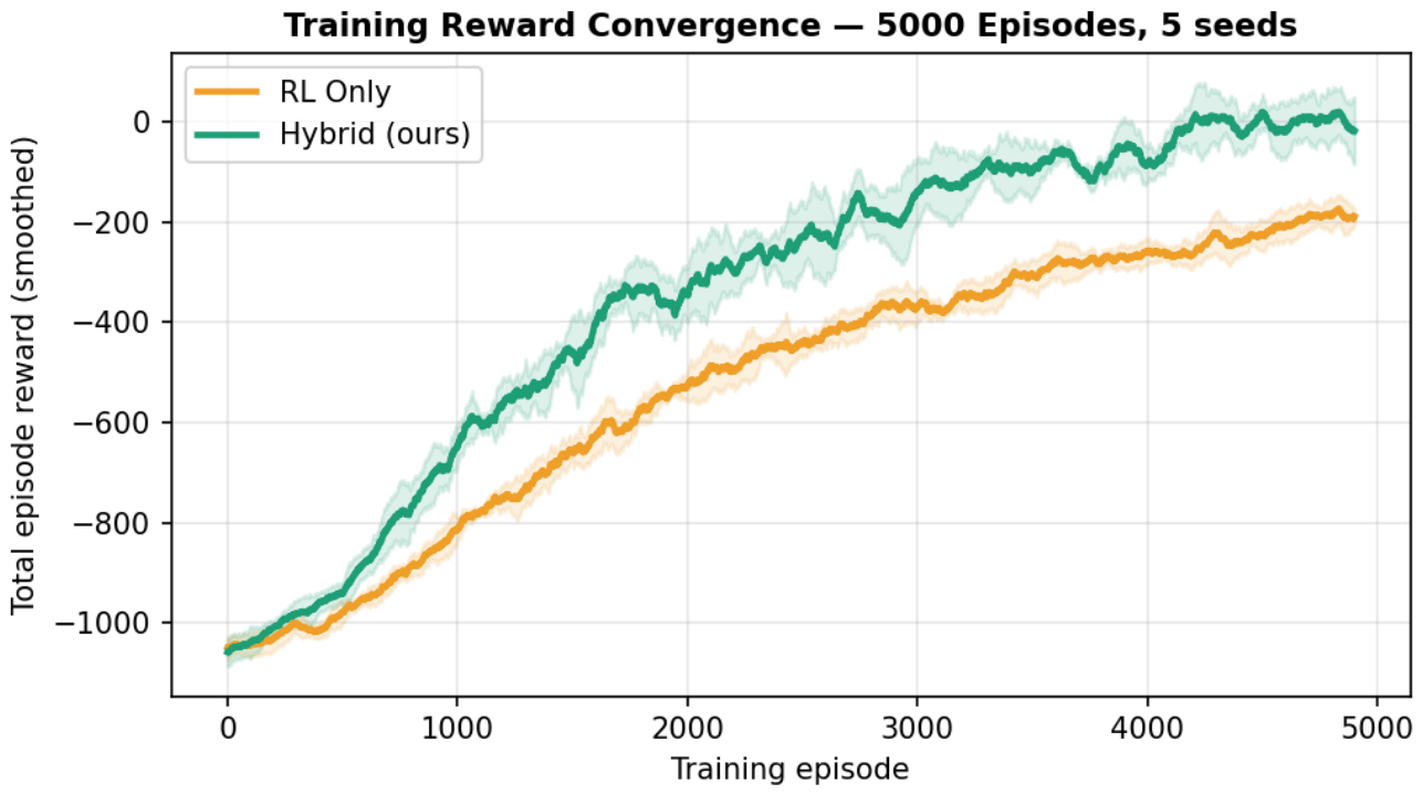
Figure 3.
Mean area coverage over 30 evaluation runs ( bands). The hybrid model achieves near-complete coverage while maintaining a learned adaptive policy.
Figure 3.
Mean area coverage over 30 evaluation runs ( bands). The hybrid model achieves near-complete coverage while maintaining a learned adaptive policy.
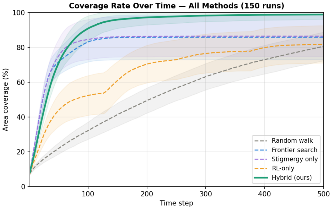
Figure 4.
Benchmark comparison over 30 runs. Lower is better for time to first victim. The hybrid model substantially outperforms RL-only in both coverage and victim detection.
Figure 4.
Benchmark comparison over 30 runs. Lower is better for time to first victim. The hybrid model substantially outperforms RL-only in both coverage and victim detection.
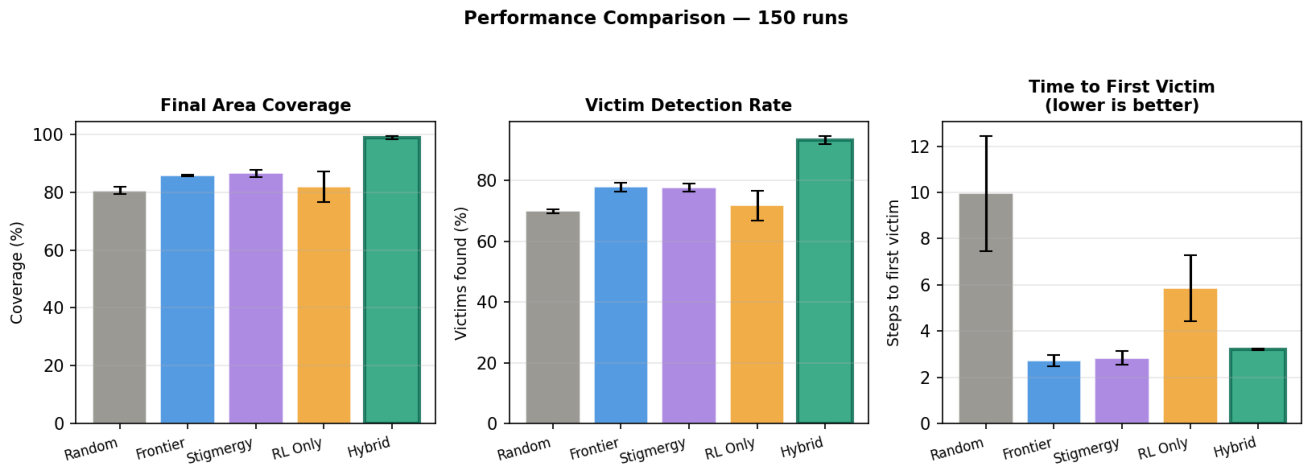
Figure 5.
Ablation study: coverage and victim detection for the full hybrid model versus models with directional gradients or neighbor density removed. Directional gradients are the dominant contributor.
Figure 5.
Ablation study: coverage and victim detection for the full hybrid model versus models with directional gradients or neighbor density removed. Directional gradients are the dominant contributor.
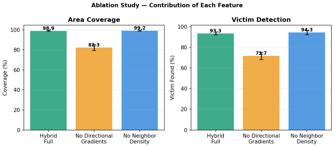
Figure 6.
Area coverage vs. communication-link failure probability (0–100%), 150 runs ( error bars). The hybrid model maintains coverage across all dropout levels, preserving a consistent –15 pp advantage over RL-only.
Figure 6.
Area coverage vs. communication-link failure probability (0–100%), 150 runs ( error bars). The hybrid model maintains coverage across all dropout levels, preserving a consistent –15 pp advantage over RL-only.
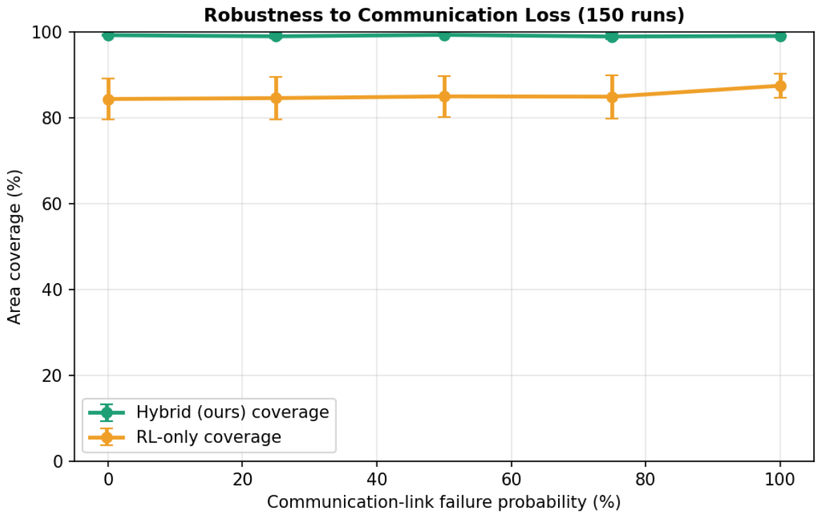

Table 1.
Comparison between scalar and directional observation representations.
| Property | Scalar | Directional |
|---|---|---|
| Spatial awareness | Limited | Enhanced |
| Decision ambiguity | High | Reduced |
| Navigation guidance | Indirect | Direct |
| Adaptability | Moderate | High |
Table 2.
Simulation Parameters and Reward Coefficients.
| Parameter | Description | Value |
|---|---|---|
| Grid / Drones / Victims | Environment setup | / 10 / 20 |
| Obstacles / Hazards | Static obstacles / hazard zones | 180 / 50 |
| Sensing radius | Per-drone view window | 2 cells |
| Comm. radius | Pheromone sharing range | 6 cells |
| Battery budget | Steps per episode | 500 |
| Evaporation rates | 0.05/0.02/0.03/0.04 | |
| Diffusion coefficients | 0.08/0.05/0.06/0.07 | |
| / | Victim / coverage weight | 5.0 / 1.0 |
| / | Comm. / energy weight | 0.3 / 0.1 |
| / | Collision / risk penalty | 2.0 / 1.5 |
| Learning rate | Q-learning step | 0.18 |
| Discount | Future reward | 0.93 |
| schedule | Exp. decay (×0.9996/ep) | at ep 5,000 |
| Discretization bins | Per pheromone feature | 6 |
| Training episodes / runs | Per agent / eval seeds | 5,000 / 30 |
Table 3.
Policy Observation State: Hybrid vs. RL-Only.
| Feature | Encoding | Hybrid | RL-only |
|---|---|---|---|
| Local coverage pheromone | 6 bins | ✓ | ✓ |
| Local victim pheromone | 6 bins | ✓ | ✓ |
| Local risk | binary flag | ✓ | ✓ |
| Normalized battery b | 4 bins | ✓ | ✓ |
| Obstacle indicators | 4 binary | ✓ | ✓ |
| Victim-gradient direction | N/S/W/E/none | ✓ | — |
| Coverage-gradient direction | N/S/W/E | ✓ | — |
| Neighbor density | 3 bins | ✓ | — |
| Total state dimension | 18 | 9 | |
Table 4.
Evaluation Results: Mean ± Std across 5 Seeds (30 Runs Each, Pooled ; grid, 10 drones, 20 victims, 500 steps).
Table 4.
Evaluation Results: Mean ± Std across 5 Seeds (30 Runs Each, Pooled ; grid, 10 drones, 20 victims, 500 steps).
| Method | Coverage (%) | Victims (%) | 1st victim (steps) |
|---|---|---|---|
| Random walk | |||
| Frontier search | |||
| Stigmergy only | |||
| RL-only | |||
| Hybrid (ours) |
Table 5.
Ablation Study — Mean ± Std across 5 Seeds (30 Runs Each, Pooled ).
| Variant | Coverage (%) | Victims (%) |
|---|---|---|
| Hybrid Full (ours) | ||
| No directional gradients | ||
| No neighbor density |
Table 6.
Communication-Dropout Sweep: Mean Coverage and Victims (%), 150 Runs.
| Dropout | Hybrid cov. | Hybrid vic. | RL cov. | RL vic. |
|---|---|---|---|---|
| 0% | 99.3 | 93.7 | 84.4 | 73.7 |
| 25% | 99.0 | 93.3 | 84.6 | 73.3 |
| 50% | 99.3 | 93.6 | 85.0 | 73.9 |
| 75% | 98.9 | 93.2 | 84.9 | 74.6 |
| 100% | 99.1 | 91.8 | 87.5 | 76.9 |
Disclaimer/Publisher’s Note: The statements, opinions and data contained in all publications are solely those of the individual author(s) and contributor(s) and not of MDPI and/or the editor(s). MDPI and/or the editor(s) disclaim responsibility for any injury to people or property resulting from any ideas, methods, instructions or products referred to in the content. |
© 2026 by the authors. Licensee MDPI, Basel, Switzerland. This article is an open access article distributed under the terms and conditions of the Creative Commons Attribution (CC BY) license (http://creativecommons.org/licenses/by/4.0/).
Copyright: This open access article is published under a Creative Commons CC BY 4.0 license, which permit the free download, distribution, and reuse, provided that the author and preprint are cited in any reuse.


