
Submitted:
25 June 2026
Posted:
26 June 2026
You are already at the latest version
Abstract
Atmospheric artifacts can obscure tectonic deformation in interferometric synthetic aperture radar (InSAR) observations, while conventional correction methods often depend on external atmospheric data. This study proposes a supervised residual-learning framework that directly predicts noise components in unwrapped InSAR maps rather than reconstructing deformation signals. Physically informed synthetic datasets were generated by combining Okada and Mogi deformation models with topography-correlated tropospheric delays, spatially correlated turbulent noise, and long-wavelength ramps. A network-depth sensitivity analysis identified a 20-layer denoising convolutional neural network as the optimal balance between accuracy and model complexity. Tests on independent synthetic datasets showed that the model reliably distinguished deformation from noise when the signal-to-noise ratio exceeded approximately 10⁻¹, whereas performance degraded under extremely noise-dominated conditions. The framework was further evaluated using ALOS/PALSAR and ALOS-2/PALSAR-2 observations of post-eruptive deformation at Mt. Ontake, Japan, and coseismic deformation associated with the 2009 L’Aquila earthquake, Italy. Compared with uncorrected, GACOS-corrected, and linear-corrected results, the CNN correction reduced topography-correlated and long-wavelength artifacts, improved temporal consistency, and generally achieved closer agreement with GNSS observations. These results demonstrate that residual noise learning offers an efficient and source-independent approach for automatic atmospheric correction of unwrapped InSAR observations.
Keywords:
InSAR
; atmospheric correction
; residual learning
; convolutional neural network
; DnCNN
; deep learning
; tropospheric delay
; surface deformation
; GNSS
1. Introduction
Interferometric Synthetic Aperture Radar (InSAR) exploits the phase difference between two Synthetic Aperture Radar (SAR) acquisitions to construct an interferogram, which describes surface displacement in the line-of-sight (LOS) direction and provides critical insight into tectonic and volcanic processes [1]. Since the early 1990s, InSAR has enabled the successful observation of coseismic deformation associated with major earthquakes, including the 1992 Landers earthquake [2,3,4,5], the 1995 Kobe earthquake in Japan [6], and the 2023 Türkiye–Syria earthquake sequence [7]. Advances in InSAR time-series techniques, such as the Small Baseline Subset (SBAS) method [8] and Permanent Scatterer InSAR (PS-InSAR) [9], have further expanded its applicability to monitoring the temporal evolution of crustal deformation. These approaches have been used to quantify interseismic strain accumulation along the southern San Andreas Fault system [10], characterize regional crustal deformation and strain in Taiwan [11], and estimate the slip deficit along the East Anatolian Fault [12]. InSAR has also contributed significantly to volcanic hazard assessment and physical interpretation, including observations of deflation at Mount Etna in 1995 [13], joint GPS–InSAR monitoring of the Nisyros Volcano between 1995 and 2002 [14], and documentation of long-term post-eruptive deflation at Mt. Ontake, Japan [15].
However, because InSAR relies on electromagnetic phase measurements, interferograms are unavoidably contaminated by various sources of noise whose amplitudes can be comparable to, or even larger than, the underlying tectonic deformation signal [16,17]. When the SAR signal propagates through the ionosphere, its polychromatic nature leads to frequency-dependent dispersion, producing ionospheric phase artifacts in the interferogram. In addition, variations in water vapor within the troposphere induce refractive path delays, generating tropospheric noise that further obscures the deformation signal. These noise sources complicate the interpretation of InSAR products and limit the broader applicability of the technique without careful correction and expert analysis. Ionospheric delays, owing to their dispersive nature, can be effectively mitigated using the range split-spectrum method (RSSM) [18]. In contrast, mitigation of tropospheric delays typically relies on external atmospheric datasets and is therefore not always reliable or effective [19].
With rapid advances in computing hardware, particularly in the development of high-performance processors, deep learning (DL) has demonstrated remarkable capabilities in image super-resolution [20,21], object detection [22,23], and image recognition [24]. In parallel, DL-based approaches have increasingly been applied to InSAR analysis for automatic noise mitigation and deformation detection. These applications include the extraction of cumulative displacement associated with fault creep and volcanic deflation [25], automated detection of volcanic surface deformation [26], identification of coseismic surface deformation [27], and autonomous noise reduction in mountainous regions [28].
Despite the growing success of deep-learning-based approaches in InSAR analysis, most existing methods are trained to map noisy interferograms directly to deformation signals, implicitly assuming that deformation patterns are sufficiently constrained or representative in the training data. However, surface deformation associated with tectonic and volcanic processes exhibits highly variable spatial characteristics across different geological settings, sensor configurations, and observation geometries. As a result, deformation-oriented training strategies may lack generalization and risk suppressing true deformation signals when applied to previously unseen scenarios.
In contrast, although atmospheric and ionospheric noise in InSAR interferograms is complex, its physical origin and statistical structure are comparatively more consistent across regions and sensors. This observation motivates a noise-oriented learning strategy, in which the model is trained to explicitly identify and extract noise components rather than to infer deformation signals. In this study, we therefore propose a supervised deep-learning framework based on residual learning that directly targets atmospheric noise in unwrapped InSAR interferograms. By training the network on physically informed synthetic datasets that separately model deformation and noise contributions, the proposed approach aims to achieve robust and tectonic source-independent noise mitigation while preserving genuine deformation signals.
The main contributions of this work are threefold. First, we reformulate InSAR denoising as a residual-learning problem focused on noise extraction, enabling improved generalization across diverse tectonic environments and SAR missions. Second, we construct a comprehensive synthetic training dataset that integrates physically based deformation models and atmospheric weather models. Third, we demonstrate that the proposed framework effectively suppresses atmospheric artifacts while retaining deformation signals under varying noise levels, as validated using independent test datasets.
This article is a revised and expanded version of a paper entitled “Automatic Detection of Tectonic Surface Deformation in InSAR Unwrapped Maps Using Deep Learning,” which was presented at the 9th Asia-Pacific Conference on Synthetic Aperture Radar (APSAR 2025), Matsue, Shimane, Japan, 5–9 October 2025 [29].
2. Materials and Methods
To mitigate atmospheric noise embedded in InSAR interferograms acquired over complex tectonic settings—and to avoid inadvertently learning the deformation signal itself—it is essential to characterize the noise directly. To this end, we adopted a supervised convolutional neural network architecture modified from the Denoising Convolutional Neural Network (DnCNN) proposed by Zhang et al. [30], which incorporates residual learning [31]. The original DnCNN is a supervised residual-learning framework designed to predict additive Gaussian noise from noisy images. In the original implementation, noisy training images are generated by adding synthetic Gaussian noise to clean images, and the network is trained to predict the corresponding noise residuals. Because Gaussian noise differs substantially from the atmospheric and ionospheric artifacts present in InSAR unwrapped interferograms, we reformulated the supervised learning architecture. Synthetic deformation fields and noise components were generated and labeled separately, enabling the model to learn the statistical characteristics of noise relevant to InSAR applications. Figure 1 illustrates the overall process of the deep learning architecture. First, we apply the Range Split-Spectrum Method [18] to reduce long-wavelength ionospheric phase screens. The interferometric phases are then unwrapped using SNAPHU [32] to convert wrapped phase (−π to π) into continuous deformation fields. The resulting unwrapped interferograms serve as input to the deep-learning model, which outputs noise-mitigated deformation maps.
Figure 1.
Schematic illustration of the CNN-based workflow for noise mitigation in InSAR interferograms, modified from [29].
Figure 1.
Schematic illustration of the CNN-based workflow for noise mitigation in InSAR interferograms, modified from [29].
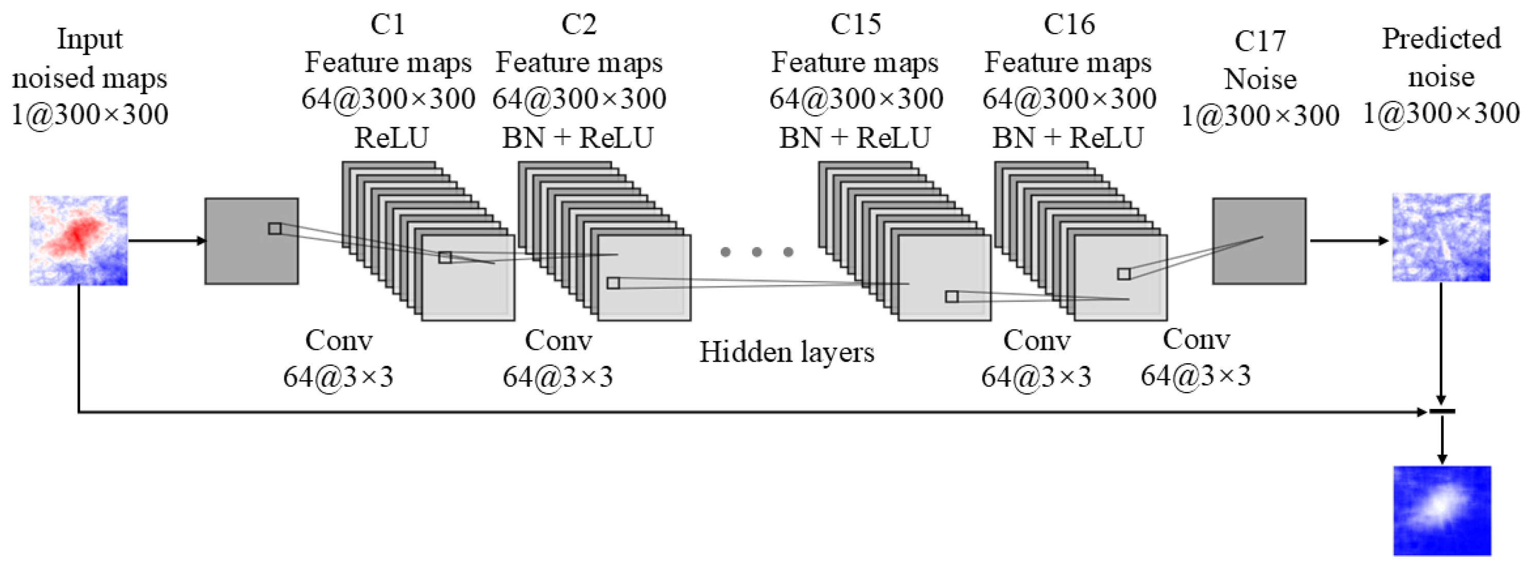
Figure 2.
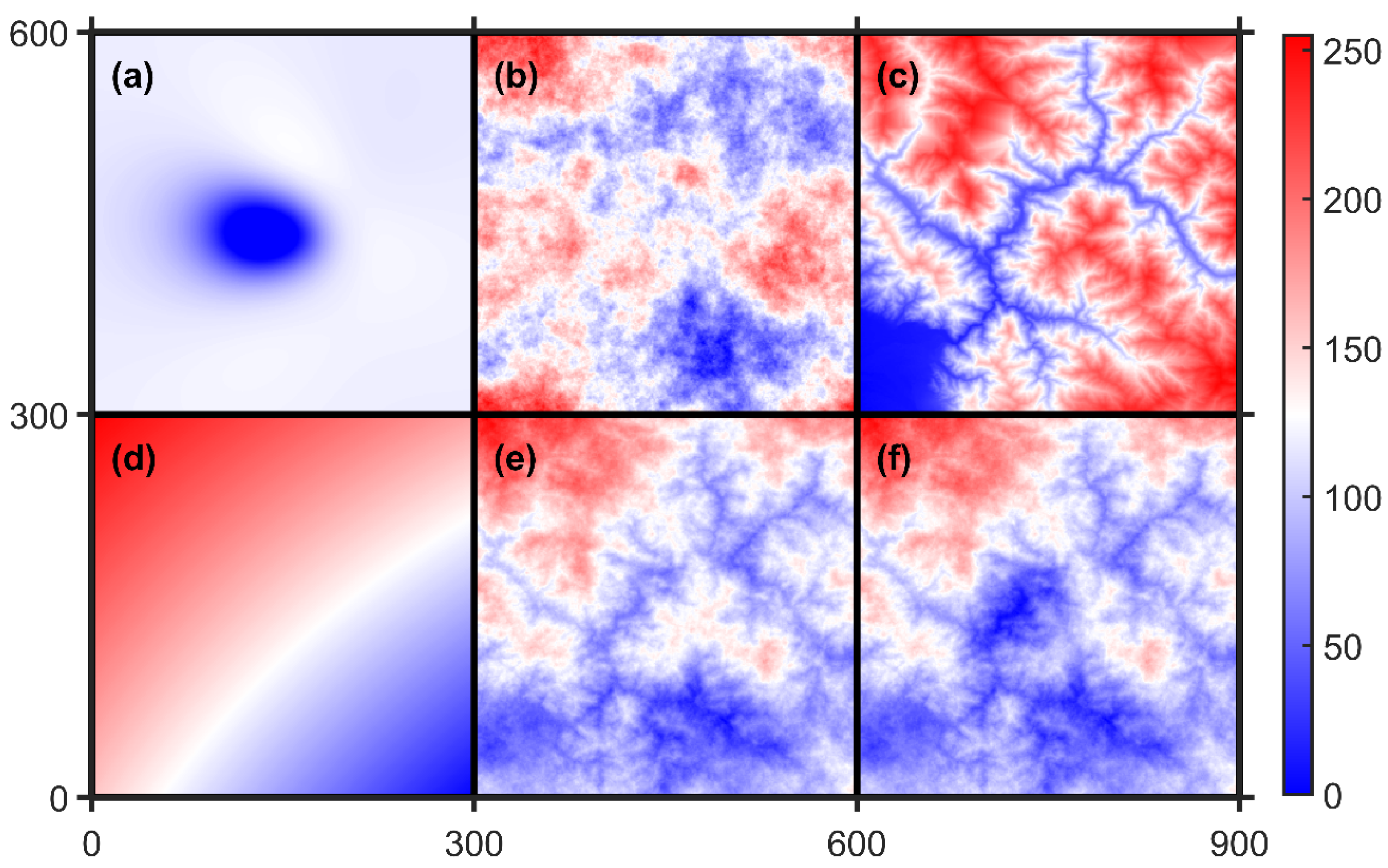
Components used to construct synthetic unwrapped interferograms. All panels are shown in 8-bit format with pixel values ranging from 0 to 255. (a) Surface deformation simulated using forward models based on the Mogi or Okada formulations. (b) Randomly generated spatially correlated exponential noise. (c) Randomly generated tropospheric delay. (d) Randomly generated bilinear ramp. (e) Synthetic noise obtained by combining components (b)–(d). (f) Final synthetic unwrapped interferogram by combining (a) and (e).
Figure 2.
Components used to construct synthetic unwrapped interferograms. All panels are shown in 8-bit format with pixel values ranging from 0 to 255. (a) Surface deformation simulated using forward models based on the Mogi or Okada formulations. (b) Randomly generated spatially correlated exponential noise. (c) Randomly generated tropospheric delay. (d) Randomly generated bilinear ramp. (e) Synthetic noise obtained by combining components (b)–(d). (f) Final synthetic unwrapped interferogram by combining (a) and (e).
2.1. Synthetic Datasets
Synthetic aperture radar (SAR) satellites operate at different wavelengths, and their interferometric phases are recorded in wrapped form (−π to π). Several recent deep-learning studies have directly used wrapped phase to perform deformation detection [27] or to suppress high-frequency noise [33]. However, even for identical deformation events at the same location, variations in radar wavelength lead to distinct statistical and spatial characteristics in the interferometric phase. To ensure robust generalization across sensors, we therefore trained our model using unwrapped phase data, enabling it to accommodate products from different SAR missions.
Because supervised learning requires many labeled samples, we constructed a synthetic dataset for training, validation, and testing. In total, we generated , , and synthetic InSAR unwrapped interferograms containing both deformation signals and atmospheric noise for training, validation, and testing. To simulate realistic atmospheric delays in the LOS direction, we followed the common assumption that tropospheric delay consists of two components: (i) a stratified term strongly correlated with local topography, and (ii) a turbulent term associated with atmospheric disturbances [34,35,36]. The stratified tropospheric component was derived using the Iterative Tropospheric Decomposition (ITD) method [37], applied to an ERA5-based Zenith Total Delay (ZTD) model [38] and the 30-m Shuttle Radar Topography Mission (SRTM) digital elevation model (DEM) [39]. The turbulent tropospheric component was generated independently as spatially correlated random noise with exponential distance-decay correlation lengths ranging from 1 to 5 km [40].
In addition to turbulent and stratified tropospheric delays, we introduced long-wavelength components by generating random bilinear ramps to mimic large-scale InSAR noise. The final synthetic noise field was constructed by combining the spatially correlated noise, the ITD-derived tropospheric delays, and the bilinear ramps.
To further constrain the model and ensure that it can reliably distinguish deformation signals from atmospheric artifacts, we generated synthetic deformation fields using forward models based on the Okada elastic dislocation solution [41] and the Mogi point-source formulation [42]. These models represent deformation associated with deeply buried fault slip and volcanic or pressure-source inflation or deflation, respectively. The simulated deformation fields were subsequently combined with the synthetic noise using random scaling factors that varied across samples to emulate a wide range of observational conditions.
For compatibility with the deep-learning architecture and to enable efficient data storage and training, all synthetic datasets were converted to 8-bit images (pixel range 0–255) using min–max normalization, as defined in Equations (2) and (3). Here, in Equation (1), the denotes the noisy unwrapped patch, the denotes the corresponding clean patch, and the represents the noise component embedded in the unwrapped interferogram. In Equations (2) and (3), and denote the maximum and minimum values of the original noisy unwrapped InSAR maps, respectively. The variables and represent the normalized input patch and the corresponding clean patch. Each synthetic InSAR unwrapped interferogram has a spatial resolution equivalent to a pixel spacing of 5.5 arcseconds and covers an area of 50 km × 50 km.
2.2. Convolutional Neural Network
As illustrated in Figure 1, a typical single-layer DnCNN architecture comprises three functional components: (i) a convolutional block, (ii) a batch-normalization block, and (iii) an activation layer. The convolutional block employs a series of 64 convolutional filters of size 3 × 3. During training, these filters convolve across the image to extract features at multiple spatial scales. Because convolution itself is a linear operation, a network composed of convolutional layers only would still be limited to a linear mapping and would be insufficient to represent the complex nonlinear characteristics of realistic InSAR noise. To overcome this limitation, the DnCNN introduces a rectified linear unit (ReLU) [43] after each convolutional layer. The ReLU function acts as a data-dependent activation mask: negative responses are suppressed, while positive responses are selectively preserved and propagated to the next layer. In this way, the network can adaptively gate features at different spatial locations and channels according to the local convolutional responses. Although each convolutional filter is linear, the repeated combination of convolution and ReLU forms a piecewise linear nonlinear mapping, enabling the network to distinguish and extract complex noise-related features across multiple spatial scales.
The DnCNN employs a residual-learning framework, in which the loss function is formulated to predict the noise component directly (Equation (4)). Here, denotes the loss between the predicted and reference noise, represents the residual predicted by the network, and denotes the trainable kernel parameters. The variables and denote the normalized clean image and the corresponding noisy image for the -th sample in a batch. Because surface deformation resulting from deep sources can exhibit diverse spatial wavelengths depending on the underlying tectonic environment, it is challenging to construct a generalizable deformation-to-deformation (source–target) mapping for noise mitigation. In contrast, although the noise embedded in unwrapped InSAR interferograms is itself complex, its statistical and spatial characteristics are comparatively more consistent across regions and sensors. This makes residual learning particularly suitable for InSAR denoising, as it allows the network to focus on learning the noise distribution rather than the deformation signal. Compared with more complex architectures such as U-Net [44], DnCNN’s streamlined design—comprising only convolutional, batch-normalization, and activation layers—substantially reduces the number of trainable parameters. At the same time, the residual-learning formulation enables direct extraction of the noise field from the input interferograms, thereby meeting our requirement for a general and efficient noise-mitigation framework.
When training, to reduce computational cost and enhance model stability, we adopted a batch size of 64 and partitioned the synthetic InSAR unwrapped interferograms into patches of 100 × 100 pixels, yielding a total of training samples. Parameter updates during back-propagation [45] were performed using the Adam optimizer [46] with an initial learning rate of 0.001. The training samples were randomly shuffled at the beginning of each epoch to reduce order-related bias and to vary the combinations of deformation and noise components presented to the network.
When validating, we selected the optimal model and prevented overfitting by incorporating early stopping during training [47]. We set a patience of 30 epochs and a tolerance threshold of 10-5. In practice, if the validation loss fails to decrease by more than this threshold for 30 consecutive epochs, the training process is considered to have converged and is terminated.
When testing, after completing the training and validation stages, we evaluated model performance using an independent test dataset. During testing, we calculated the structural similarity index (SSIM; Equation (5)) and the signal-to-noise ratio (SNR; Equation (6)) to evaluate model performance under different noise levels, where in Equation (5), and denote the mean values of the reference and predicted clean images, respectively; and denote their corresponding standard deviations; and and are constants used to stabilize the calculation. In Equation (6), and represent the powers of the reference clean image and the synthetic noise, respectively. To prevent data leakage and ensure a rigorous assessment, the training, validation, and testing datasets were generated from non-overlapping geographic regions of the SRTM topography. Specifically, the training dataset was constructed within the domain [54°E–120°E, 26°N–37°N], the testing dataset within [70°E–110°E, 40°N–50°N], and the validation dataset within [100°W–120°W, 37°N–46°N].
2.3. Data Augmentation
Data augmentation is an effective strategy in deep-learning training, yielding average accuracy improvements of approximately 20% through operations such as cropping, flipping, and rotation [48]. Following this rationale, we applied random flipping and rotation to the training dataset to vary the relative spatial arrangement between noise and deformation components before model input. In addition, the original training samples were rescaled using cubic interpolation with scale factors of 0.7, 0.8, 0.9, and 1.0, resulting in patch sizes of , , , and pixels. Data augmentation was applied exclusively to the training dataset. It was not used for the validation or test datasets, which were kept fixed to ensure consistency in model monitoring and performance evaluation.
3. Results
Before applying the deep-learning model to real case studies, we conducted comprehensive training and evaluation experiments. In this section, we first performed a sensitivity analysis of the network depth using the training dataset. We then carried out the training and validation processes simultaneously to identify the optimal model configuration. Finally, model performance was assessed by examining the relationship between the Structural Similarity Index (SSIM) and the signal-to-noise ratio (SNR). All training procedures were performed on an NVIDIA RTX 3090 GPU.
3.1. Sensitivity Analysis of Network Depth
After constructing the datasets for training, validation, and testing, we determined the key hyperparameters required for model training. The number of training epochs was controlled using an early-stopping strategy, whereby performance on the validation dataset was monitored to identify the optimal stopping point. For batch-size selection, previous studies have shown that larger batch sizes produce smoother validation loss curves and improve optimization stability [49]. In addition, larger batch sizes help mitigate internal covariate shift, which can hinder convergence in deep neural networks [50]. Accordingly, we adopted a batch size of 64, the maximum supported by our GPU, for both training and validation to enhance convergence efficiency and reduce validation fluctuations. The learning rate was managed using the adaptive Adam optimizer, which dynamically adjusts the learning rate during training. Consequently, the primary hyperparameter requiring sensitivity analysis in this study is the depth of the DnCNN architecture.
To evaluate the impact of network depth on model performance, we tested DnCNN architectures with 5, 10, 15, 17, 20, and 25 layers, including the original 17-layer configuration. Each model was trained and evaluated on the validation dataset, and its minimum validation loss was determined under the early-stopping criterion. We assume that when the difference in minimum validation loss between two consecutive depth configurations is less than 1 × 10⁻³, further increases in network depth do not lead to a meaningful improvement in performance.
Figure 3 presents the training and validation loss curves for models with different depths, while Figure 4 summarizes the corresponding minimum validation losses. When the network depth exceeds 15 layers, further increases result in only marginal changes in convergence behavior. Extending the depth to 25 layers leads to clear signs of overfitting during validation, whereas the training loss continues to decrease without reaching convergence. The minimum validation losses were 0.0460, 0.0432, 0.0414, 0.0408, 0.0404, and 0.0397 for models with 5, 10, 15, 17, 20, and 25 layers, respectively. Because the loss reduction between the 20-layer and 25-layer configurations is only 0.0007—below the predefined threshold—we selected the 20-layer model as the optimal DnCNN architecture. Based on the early-stopping criterion, the final 20-layer model converged after 63 training epochs.
3.2. Performance Evaluation on Synthetic Data
After completing the sensitivity analysis of the DnCNN hyperparameters and the training, we evaluated model performance on the test dataset by examining the variation of the Structural Similarity Index (SSIM) as a function of the signal-to-noise ratio (SNR), as illustrated in Figure 5. The heatmap reveals an overall decreasing trend in SSIM with decreasing SNR, with a pronounced transition occurring near an SNR in the range of 10-1 to 10-2, suggesting that the model largely loses its ability to distinguish deformation signals from noise in the unwrapped interferograms. The results indicate that performance decreases markedly when the noise power exceeds the signal power by approximately one to two orders of magnitude.
3.3. Application to Real InSAR Observations
3.3.1. Application in the Post-Eruption Period of Mount Ontake, Japan
Mount Ontake, located in central Japan, has experienced four documented phreatic eruptions in 1979, 1991, 2007, and 2014. Since the 1990s, rapid advances in geodetic monitoring techniques have enabled near–real-time observations of crustal deformation associated with volcanic activity, providing critical constraints on subsurface processes. In particular, the 2014 eruption of Mt. Ontake was extensively observed using both Global Navigation Satellite System (GNSS) and Interferometric Synthetic Aperture Radar (InSAR) data. Using ALOS-2/PALSAR-2 observations, Narita et al. [15] reported the LOS deformation rates of approximately 21 cm/yr and 12 cm/yr for ascending and descending Stacking-InSAR [51,52] analyses, respectively. However, the complex topography of the study area (Figure 6), combined with seasonal snow cover and dense vegetation, introduces strong temporal variability in atmospheric noise, which substantially contaminates the deformation signal in individual interferograms. These characteristics make the study area well-suited for evaluating the performance of the proposed automatic denoising framework.
3.3.2. Preprocessing for InSAR Interferogram Generation
To evaluate the performance of the proposed deep-learning model on real InSAR data, we selected interferograms covering the Mt. Ontake region, as shown in the study-area map in Figure 6. The data were provided by the Japan Aerospace Exploration Agency (JAXA) and correspond to path–frame 20–2890 on the descending orbit, spanning the period from October 2014 to October 2017.
Interferogram generation and preprocessing were conducted using the open-source GMTSAR software package [53]. Specifically, interferograms were generated, and the range split-spectrum method (RSSM) [18] was applied to mitigate dispersive long-wavelength ionospheric components. The interferometric phases were subsequently unwrapped using the SNAPHU algorithm [32]. From the original 15 descending SAR acquisitions, a total of 59 unwrapped interferograms were generated, as shown in Table 1.
3.3.3. CNN-Based Atmospheric Correction
The 59 interferograms were subsequently processed using the Small Baseline Subset (SBAS) algorithm to derive 15 deformation time-series maps corresponding to the original 15 Single Look Complex (SLC) images, which are focused Synthetic Aperture Radar (SAR) products in which each pixel is represented as a complex number consisting of in-phase and quadrature components. These unwrapped InSAR time-series maps were then input into the trained deep-learning architecture to generate CNN-corrected deformation maps for each epoch.
To compare the performance of the proposed approach with conventional correction methods, we additionally applied two widely used atmospheric correction techniques to each interferogram: (1) Zenith Total Delay (ZTD) correction using the Generic Atmospheric Correction Online Service for InSAR (GACOS) [54], and (2) a height-dependent phase correction based on the bilinear relationship between the unwrapped phase and the digital elevation model (DEM) [55]. The same InSAR time-series processing workflow was subsequently applied to all corrected datasets.
As shown in Figure 7b, the CNN-corrected time-series maps suppress most of the DEM-correlated stratified atmospheric delays present in the original interferograms, whereas substantial residual artifacts remain in the GACOS-corrected and linear-corrected results (Figure 7c and Figure 7d). In addition, several long-wavelength artifacts are further reduced after CNN correction, particularly in the deformation map corresponding to 7 August 2016.
To further evaluate the effectiveness of the proposed model, the unwrapped deformation time series were converted into velocity fields using least-squares regression. As shown in Figure 8, the CNN-corrected velocity field (Figure 8b) exhibits substantially reduced topography-correlated artifacts compared with the uncorrected, GACOS-corrected, and linear-corrected results (Figure 8a, Figure 8c and Figure 8d). These observations are consistent with the improvements observed in the time-series deformation maps.
In addition, standard error maps were estimated simultaneously with the velocity fields, as shown in Figure 9. The CNN-corrected velocity field exhibits the lowest mean standard error (±2.96 mm/yr), compared with ±5.10 mm/yr, ±4.49 mm/yr, and ±4.92 mm/yr for the uncorrected, GACOS-corrected, and linear-corrected results, respectively. The reduced standard errors indicate that the CNN correction improves the temporal consistency of the deformation estimates and suppresses fluctuations in the time-series observations across most pixels.
3.3.4. Comparison with GNSS Time Series
In addition to the comparison with existing atmospheric correction methods, we further evaluated the temporal stability of the CNN-corrected results using continuous GNSS observations. Specifically, the uncorrected, GACOS-corrected, linear-corrected, and CNN-corrected InSAR time series were compared with continuous GNSS time series from nine nearby stations operated by the Geospatial Information Authority of Japan (GSI). The GNSS observations span the period from October 2014 to October 2017, corresponding to the same time interval as the InSAR time series. The locations of the GNSS stations are shown in Figure 6.
To ensure a consistent reference frame, all InSAR and GNSS displacement time series were referenced to station 960614 (137.60°E, 35.88°N). The GNSS displacement time series were subsequently projected from the east–north–up (ENU) coordinate system into the satellite LOS direction using Equation (7), where denotes the displacement in the LOS direction, , and represent the displacement components in the north, east, and vertical directions, respectively. The parameters and denote the satellite azimuth and incidence angles, respectively.
The LOS displacement time series derived from GNSS and the four InSAR datasets are compared in Figure 10. At most stations, the CNN-corrected InSAR time series exhibits the closest agreement with the GNSS observations relative to the uncorrected, GACOS-corrected, and linear-corrected results. To quantify the agreement, the root mean square error (RMSE) was calculated for each station, as shown in Figure 11. Except for station 960611, the CNN-corrected results yield the lowest RMSE values among the four InSAR datasets, indicating improved consistency with the GNSS time series.
3.4. Application to a Coseismic Interferogram
The central Apennines of Italy are characterized by a complex fault system formed during the Quaternary because of N–S compressional tectonics and NW–SE extension associated with shear interactions between the subducting lithosphere and the underlying mantle [56]. Paleoseismological studies indicate a recurrence interval of approximately 1000–2000 years for earthquakes of magnitude 7 or greater since 1200 AD [57]. In addition, statistical analyses of seismic catalogs from 1987 to 2000, based on the Gutenberg–Richter relationship with b-values close to 1, suggest a recurrence interval of approximately 150 years for magnitude 6 events [58]. Both paleoseismological and seismic analyses indicate a high potential for destructive earthquakes in this region.
On 6 April 2009 at 01:32:39 UTC, the city of L’Aquila in the central Apennines was struck by a Mw 6.3 earthquake. The event generated widespread normal-faulting deformation across the surrounding region and resulted in 307 fatalities, making it one of the most destructive earthquakes in modern Italian history.
Previous studies have investigated the source mechanism of the 2009 L’Aquila earthquake using GNSS observations [59]. However, the presence of multiple error sources in InSAR data complicates direct comparisons with GNSS measurements. To improve the consistency between the two datasets, previous studies often restricted their analyses to a relatively small area surrounding the epicenter, thereby minimizing atmospheric and orbital artifacts. Therefore, deformation signals outside the selected region were excluded from the analysis.
3.4.1. CNN-Based Correction and GNSS Validation
In this study, we applied the same preprocessing workflow to an ALOS/PALSAR interferometric pair from path–frame 639–840, as shown in Table 1, to generate an unwrapped interferogram with a mask factor of 0.1. The resulting unwrapped map was then input into the trained deep-learning model for noise mitigation. The unwrapped interferograms before and after CNN correction are shown in Figure 12.
Compared with the original unwrapped interferogram (Figure 12b), the CNN-corrected result (Figure 12c) exhibits a substantial reduction in the NE–SW-oriented long-wavelength ramp. In addition, short-wavelength artifacts are effectively suppressed after correction, resulting in a cleaner deformation field and improved spatial continuity of the coseismic signal.
We further projected the GNSS displacement measurements reported by Anzidei et al. [59] into the LOS direction using Equation (7) to enable direct comparison with the InSAR-derived coseismic displacements before and after CNN correction. Both the GNSS and InSAR observations were referenced to the SELL station.
As shown in Figure 13, the absolute differences between the GNSS and InSAR coseismic displacements were calculated for each station. The CNN-corrected results exhibit consistently smaller differences than the uncorrected observations at all stations. The improved agreement between the GNSS and InSAR measurements provides independent validation of the effectiveness of the proposed CNN-based approach for noise mitigation in coseismic InSAR interferograms.
4. Discussion
4.1. Merits and Distinctive Features of the Proposed Method
Previous studies have primarily focused on reconstructing tectonic deformation signals. However, deformation patterns vary substantially among different tectonic settings because of the diverse source mechanisms underlying earthquakes, volcanic activity, and other geodynamic processes. In contrast, although atmospheric noise in InSAR interferograms is also complex, based on the assumption in this study, its constituent components and statistical characteristics are relatively more constrained. By introducing residual learning to directly predict noise rather than deformation, the proposed framework offers improved generalization across diverse tectonic environments. Furthermore, as summarized in Table 2, the relatively simple architecture and reduced number of trainable parameters enhance computational efficiency and facilitate deployment on a wider range of hardware platforms.
4.2. Effects of Interferometric Coherence on Prediction Performance
Although multiple noise sources were incorporated into the synthetic training datasets, real InSAR interferograms contain error sources that are considerably more complex than those represented in the simulations. In particular, low-quality interferometric phases caused by decorrelation, layover, or shadowing can introduce phase residues and local inconsistencies, which may subsequently propagate into large-scale phase-unwrapping errors [60]. Furthermore, previous studies have demonstrated that phase-unwrapping reliability is strongly related to interferometric coherence. Statistical phase-unwrapping algorithms estimate the most probable unwrapped phase field based on observable quantities, assigning lower confidence to regions with poor phase quality or low coherence during the optimization process [32].
Coherence-related phase-unwrapping errors, together with localized artifacts caused by geometric distortions in the satellite viewing geometry, are difficult to distinguish from genuine deformation signals based on either their statistical characteristics or their spatial patterns. Consequently, the deep-learning model may occasionally interpret these artifacts as deformation signals, leading to erroneous predictions.
This limitation is also evident in our results. When comparing the four correction methods against the GNSS LOS displacement time series, station 960611 is the only station at which the CNN-corrected result exhibits a larger RMSE than the uncorrected, GACOS-corrected, and linear-corrected results. To investigate the cause of this anomalous prediction, we calculated the mean coherence map from all 59 interferograms of path–frame 20–2890 used in the Mt. Ontake case study.
As shown in Figure 14, the coherence distribution exhibits a pronounced NE–SW trend, with coherence gradually increasing from the northeastern to the southwestern part of the study area. To further quantify the spatial variability of coherence, a Delaunay triangulation network [61] was constructed using the nine GNSS stations, and the mean coherence within each triangular region was calculated. The triangle containing station 960611 exhibits the lowest mean coherence value (0.14713) among all regions. This result indicates that the InSAR observations associated with station 960611 are strongly affected by decorrelation, making them more susceptible to phase-unwrapping errors and reducing the reliability of the CNN prediction.
The low-coherence environment surrounding station 960611 likely contributes to coherence-related phase-unwrapping errors and localized artifacts. Because these artifacts may exhibit spatial and statistical characteristics similar to those of genuine deformation signals, they are difficult to distinguish from true deformation. Consequently, the deep-learning model may incorrectly interpret these artifacts as deformation signals, leading to degraded prediction performance at this station.
4.3. Performance Degradation in Real Interferograms
As demonstrated in Figure 5, the performance of the proposed model decreases substantially when the SNR falls from approximately 10-1 to 10-2. In practical applications, however, the noise level of a real interferogram is generally unknown, making it difficult to estimate the corresponding SNR. Moreover, atmospheric, orbital, and processing-related noise is present to some extent in nearly all interferograms generated from SAR image pairs. Consequently, subtle deformation signals with amplitudes below the effective SNR threshold may remain indistinguishable from noise.
In such cases, additional preprocessing techniques, such as temporal stacking or time-series analysis, may still be required to enhance the signal-to-noise ratio before applying deep-learning-based denoising. These approaches can suppress temporally uncorrelated noise while preserving persistent deformation signals, thereby improving the separability between deformation and noise.
Therefore, although the proposed model demonstrates promising generalization capability across different tectonic settings, achieving an optimal balance between model generalization and denoising performance remains a significant challenge for the broader application of deep learning in InSAR analysis.
5. Conclusions
In this study, we developed a supervised deep-learning framework for mitigating atmospheric noise in InSAR unwrapped phase maps. Unlike conventional deformation-oriented approaches, the proposed method reformulates InSAR denoising as a residual-learning problem, allowing the CNN to directly learn and extract noise components while preserving the underlying deformation signal. Physically informed synthetic datasets were constructed by combining deformation fields generated from Okada and Mogi source models with multiple noise components, including spatially correlated turbulent noise, topography-related tropospheric delays, and long-wavelength ramp artifacts. This design enabled the model to learn realistic noise characteristics under diverse observational conditions.
A depth-sensitivity analysis showed that the 20-layer DnCNN provided the best balance between denoising performance and model complexity. Although deeper networks slightly reduced the training loss, the improvement from 20 to 25 layers was marginal and accompanied by signs of overfitting. Performance tests using independent synthetic datasets further demonstrated that the model can effectively distinguish deformation from noise when the signal-to-noise ratio remains above a critical threshold, while its reliability decreases under extremely low-SNR conditions.
The proposed framework was further applied to real ALOS-2/PALSAR-2 interferograms covering the post-eruptive deformation of Mt. Ontake. Compared with uncorrected, GACOS-corrected, and linear-corrected results, the CNN-corrected time series and velocity fields showed substantially reduced topography-correlated atmospheric artifacts and improved temporal consistency. The CNN correction produced the lowest mean standard error and generally achieved better agreement with GNSS-derived LOS displacement time series. Application to the 2009 L’Aquila earthquake also confirmed that the trained model can reduce atmospheric artifacts while retaining coseismic deformation signals.
Overall, these results indicate that residual-learning-based CNNs offer a promising and efficient approach for automatic atmospheric noise mitigation in InSAR unwrapped maps. However, model performance remains limited when deformation signals are much weaker than noise, suggesting that future work should combine deep learning with time-series stacking or other noise-suppression strategies for more robust application to low-SNR real-world interferograms.
Author Contributions
Y.L.: conceptualization, methodology, software, validation, formal analysis, investigation, data curation, writing—original draft preparation, writing—review and editing, and visualization. T.S.: conceptualization, methodology, validation, resources, writing—review and editing, supervision, project administration, and funding acquisition. All authors have read and agreed to the published version of the manuscript.
Funding
This research was funded by the Japan Science and Technology Agency (JST) through the Make New Standards Program for the Next Generation Researchers (M240020), and by the Japan Society for the Promotion of Science (JSPS) KAKENHI (JP23H01270).
Data Availability Statement
The ALOS/PALSAR SAR data used in this study are publicly available from the Alaska Satellite Facility Distributed Active Archive Center (ASF DAAC) through the ASF Vertex data portal (https://search.asf.alaska.edu/, accessed on 15 January 2026). The Shuttle Radar Topography Mission Global 1 Arc-Second digital elevation model (SRTMGL1, approximately 30 m spatial resolution) is available from the NASA Land Processes Distributed Active Archive Center (https://lpdaac.usgs.gov/products/srtmgl1v003/, accessed on 8 February 2026). The tropospheric delay products used for atmospheric correction are available from the Generic Atmospheric Correction Online Service for InSAR (GACOS; https://www.gacos.net/, accessed on 20 March 2026). The source parameters used to generate the synthetic deformation field for the 2009 L’Aquila earthquake were obtained from Anzidei et al. (2009; https://doi.org/10.1029/2009GL039145). The Hourly Global Pressure and Temperature (HGPT) model used to generate the stratified atmospheric delay components is described by Mateus et al. (2020; https://doi.org/10.3390/rs12071098). The synthetic datasets and processed results generated in this study are available from the corresponding author upon reasonable request.
Acknowledgments
The authors gratefully acknowledge the PIXEL group for providing the ALOS-2/PALSAR-2 data used in this study. The PALSAR-2 data were provided by the Japan Aerospace Exploration Agency (JAXA) under a joint research agreement with the PIXEL group (research project 2024-B-03). The GNSS data were obtained from the publicly available GEONET database maintained by the Geospatial Information Authority of Japan (GSI). The authors also thank Mateus et al. (2020) for providing the ERA5-based Hourly Global Pressure and Temperature (HGPT) model and Anzidei et al. (2009) for providing the GNSS displacement data. The authors appreciate the participants of the EGU General Assembly 2026 and the JpGU-AGU Joint Meeting 2026 for their valuable discussions, comments, and suggestions following the presentation of this work.
Conflicts of Interest
The authors declare no conflict of interest.
References
- Bürgmann, R.; Rosen, P.A.; Fielding, E.J. Synthetic aperture radar interferometry to measure Earth’s surface topography and its deformation. Annu. Rev. Earth Planet. Sci. 2000, 28, 169–209. [Google Scholar] [CrossRef]
- Massonnet, D.; Rossi, M.; Carmona, C.; Adragna, F.; Peltzer, G.; Feigl, K.; Rabaute, T. The displacement field of the Landers earthquake mapped by radar interferometry. Nature 1993, 364, 138–142. [Google Scholar] [CrossRef]
- Peltzer, G.; Rosen, P.; Rogez, F.; Hudnut, K. Poroelastic rebound along the Landers 1992 earthquake surface rupture. J. Geophys. Res. Solid Earth 1998, 103, 30131–30145. [Google Scholar] [CrossRef]
- Zebker, H.A.; Rosen, P.A.; Goldstein, R.M.; Gabriel, A.; Werner, C.L. On the derivation of coseismic displacement fields using differential radar interferometry: The Landers earthquake. J. Geophys. Res. Solid Earth 1994, 99, 19617–19634. [Google Scholar] [CrossRef]
- Price, E.J.; Sandwell, D.T. Small-scale deformations associated with the 1992 Landers, California, earthquake mapped by synthetic aperture radar interferometry phase gradients. J. Geophys. Res. Solid Earth 1998, 103, 27001–27016. [Google Scholar] [CrossRef]
- Ozawa, S.; Murakami, M.; Fujiwara, S.; Tobita, M. Synthetic aperture radar interferogram of the 1995 Kobe earthquake and its geodetic inversion. Geophys. Res. Lett. 1997, 24, 2327–2330. [Google Scholar] [CrossRef]
- Jia, Z.; Jin, Z.; Marchandon, M.; Ulrich, T.; Gabriel, A.-A.; Fan, W.; Shearer, P.; Zou, X.; Rekoske, J.; Bulut, F. The complex dynamics of the 2023 Kahramanmaraş, Turkey, Mw 7.8–7.7 earthquake doublet. Science 2023, 381, 985–990. [Google Scholar] [CrossRef] [PubMed]
- Berardino, P.; Fornaro, G.; Lanari, R.; Sansosti, E. A new algorithm for surface deformation monitoring based on small baseline differential SAR interferograms. IEEE Trans. Geosci. Remote Sens. 2002, 40, 2375–2383. [Google Scholar] [CrossRef]
- Ferretti, A.; Prati, C.; Rocca, F. Permanent scatterers in SAR interferometry. IEEE Trans. Geosci. Remote Sens. 2001, 39, 8–20. [Google Scholar] [CrossRef]
- Fialko, Y. Interseismic strain accumulation and the earthquake potential on the southern San Andreas Fault system. Nature 2006, 441, 968–971. [Google Scholar] [CrossRef] [PubMed]
- Franklin, K.R.; Huang, M.-H. Revealing crustal deformation and strain rate in Taiwan using InSAR and GNSS. Geophys. Res. Lett. 2022, 49, e2022GL101306. [Google Scholar] [CrossRef]
- Han, B.; Yu, C.; Li, Z.; et al. Slip complementarity and deficit of the East Anatolian Fault revealed by geodetic observations. Commun. Earth Environ. 2025, 6, 1053. [Google Scholar] [CrossRef]
- Massonnet, D.; Briole, P.; Arnaud, A. Deflation of Mount Etna monitored by spaceborne radar interferometry. Nature 1995, 375, 567–570. [Google Scholar] [CrossRef]
- Lagios, E.; Sakkas, V.; Parcharidis, I.; Dietrich, V. Ground deformation of Nisyros Volcano, Greece, for the period 1995–2002: Results from DInSAR and DGPS observations. Bull. Volcanol. 2005, 68, 201–214. [Google Scholar] [CrossRef]
- Narita, S.; Murakami, M. Shallow hydrothermal reservoir inferred from post-eruptive deflation at Ontake Volcano as revealed by PALSAR-2 InSAR. Earth Plan. Space 2018, 70, 191. [Google Scholar] [CrossRef]
- Chaussard, E.; Bürgmann, R.; Fattahi, H.; Nadeau, R.M.; Taira, T.; Johnson, C.W.; Johanson, I. Potential for larger earthquakes in the East San Francisco Bay Area due to the direct connection between the Hayward and Calaveras faults. Geophys. Res. Lett. 2015, 42, 2734–2741. [Google Scholar] [CrossRef]
- Khoshmanesh, M.; Shirzaei, M.; Nadeau, R.M. Time-dependent model of aseismic slip on the central San Andreas Fault from InSAR time series and repeating earthquakes. J. Geophys. Res. Solid Earth 2018, 123, 2802–2818. [Google Scholar] [CrossRef]
- Gomba, G.; Parizzi, A.; De Zan, F.; Eineder, M.; Bamler, R. Toward operational compensation of ionospheric effects in SAR interferograms: The split-spectrum method. IEEE Trans. Geosci. Remote Sens. 2016, 54, 1446–1461. [Google Scholar] [CrossRef]
- Morishita, Y.; Lazecký, M.; Wright, T.J.; Weiss, J.R.; Elliott, J.R.; Hooper, A. LiCSBAS: An open-source InSAR time series analysis package integrated with the LiCSAR automated Sentinel-1 InSAR processor. Remote Sens. 2020, 12, 424. [Google Scholar] [CrossRef]
- Alzubaidi, L.; Zhang, J.; Humaidi, A.J.; Al-Dujaili, A.; Duan, Y.; Al-Shamma, O.; Santamaría, J.; Fadhel, M.A.; Al-Amidie, M.; Farhan, L. Review of deep learning: Concepts, CNN architectures, challenges, applications, future directions. J. Big Data 2021, 8, 53. [Google Scholar] [CrossRef] [PubMed]
- Yang, W.; Zhang, X.; Tian, Y.; Wang, W.; Xue, J.-H.; Liao, Q. Deep learning for single image super-resolution: A brief review. IEEE Trans. Multimed. 2019, 21, 3106–3121. [Google Scholar] [CrossRef]
- Tang, S.; Andriluka, M.; Andres, B.; Schiele, B. Multiple people tracking by lifted multicut and person re-identification. In Proceedings of the IEEE Conference on Computer Vision and Pattern Recognition, Honolulu, HI, USA, 21–26 July 2017; pp. 3539–3548. [Google Scholar]
- Zhao, Z.-Q.; Zheng, P.; Xu, S.-T.; Wu, X. Object detection with deep learning: A review. IEEE Trans. Neural Netw. Learn. Syst. 2019, 30, 3212–3232. [Google Scholar] [CrossRef] [PubMed]
- Krizhevsky, A.; Sutskever, I.; Hinton, G.E. ImageNet classification with deep convolutional neural networks. Commun. ACM 2017, 60, 84–90. [Google Scholar] [CrossRef]
- Rouet-Leduc, B.; Jolivet, R.; Dalaison, M.; Johnson, P.A.; Hulbert, C. Autonomous extraction of millimeter-scale deformation in InSAR time series using deep learning. Nat. Commun. 2021, 12, 6480. [Google Scholar] [CrossRef] [PubMed]
- Sun, J.; Wauthier, C.; Stephens, K.; Gervais, M.; Cervone, G.; La Femina, P.; Higgins, M. Automatic detection of volcanic surface deformation using deep learning. J. Geophys. Res. Solid Earth 2020, 125, e2020JB019840. [Google Scholar] [CrossRef]
- Brengman, C.M.J.; Barnhart, W.D. Identification of surface deformation in InSAR using machine learning. Geochem. Geophys. Geosyst. 2021, 22, e2020GC009204. [Google Scholar] [CrossRef]
- Brencher, G.; Henderson, S.T.; Shean, D.E. Removing atmospheric noise from InSAR interferograms in mountainous regions with a convolutional neural network. Comput. Geosci. 2024, 192, 105771. [Google Scholar] [CrossRef]
- Li, Y.; Sagiya, T. Automatic detection of tectonic surface deformation in InSAR unwrapped maps using deep learning. In Proceedings of the 2025 9th Asia-Pacific Conference on Synthetic Aperture Radar (APSAR), Matsue, Japan, 2025; pp. 1–4. [Google Scholar] [CrossRef]
- Zhang, K.; Zuo, W.; Chen, Y.; Meng, D.; Zhang, L. Beyond a Gaussian denoiser: Residual learning of deep CNN for image denoising. IEEE Trans. Image Process. 2017, 26, 3142–3155. [Google Scholar] [CrossRef] [PubMed]
- He, K.; Zhang, X.; Ren, S.; Sun, J. Deep residual learning for image recognition. In Proceedings of the IEEE Conference on Computer Vision and Pattern Recognition, Las Vegas, NV, USA, 27–30 June 2016; pp. 770–778. [Google Scholar] [CrossRef]
- Chen, C.W.; Zebker, H.A. Two-dimensional phase unwrapping with use of statistical models for cost functions in nonlinear optimization. J. Opt. Soc. Am. A 2001, 18, 338–351. [Google Scholar] [CrossRef] [PubMed]
- Li, S.; Xu, H.; Liu, S.; Yang, J. An interferometric phase noise reduction method based on deep convolutional neural networks. IEEE J. Sel. Top. Appl. Earth Obs. Remote Sens. 2020, 13, 4940–4952. [Google Scholar]
- Williams, S.; Bock, Y.; Fang, P.; Jamason, P.; Nikolaidis, R.M.; Prawirodirdjo, L.; Miller, M.; Johnson, D.J. Integrated satellite interferometry: Tropospheric noise, GPS estimates and implications for interferometric synthetic aperture radar products. J. Geophys. Res. Solid Earth 1998, 103, 27051–27067. [Google Scholar] [CrossRef]
- Cho, J.; Newell, R.E.; Anderson, B.E.; Barrick, J.D.W.; Thornhill, K.L. Characterizations of tropospheric turbulence and stability layers from aircraft observations. J. Geophys. Res. Atmos. 2003, 108, 8784. [Google Scholar] [CrossRef]
- Li, Z.; Muller, J.-P.; Cross, P.; Albert, P.; Fischer, J.; Bennartz, R. Assessment of the potential of MERIS near-infrared water vapour products to correct ASAR interferometric measurements. Int. J. Remote Sens. 2006, 27, 349–365. [Google Scholar] [CrossRef]
- Yu, C.; Li, Z.; Penna, N.T. Interferometric synthetic aperture radar atmospheric correction using a GPS-based iterative tropospheric decomposition model. Remote Sens. Environ. 2018, 204, 109–121. [Google Scholar] [CrossRef]
- Mateus, P.; Catalão, J.; Nico, G. Sentinel-1 interferometric SAR mapping of precipitable water vapor over a country-spanning area. Remote Sens. 2020, 12, 1098. [Google Scholar] [CrossRef]
- Rabus, B.; Eineder, M.; Roth, A.; Bamler, R. The Shuttle Radar Topography Mission—A new class of digital elevation models acquired by spaceborne radar. ISPRS J. Photogramm. Remote Sens. 2003, 57, 241–262. [Google Scholar] [CrossRef]
- Lohman, R.B.; Simons, M. Some thoughts on the use of InSAR data to constrain models of surface deformation: Noise structure and data downsampling. Geochem. Geophys. Geosyst. 2005, 6, Q01007. [Google Scholar] [CrossRef]
- Okada, Y. Surface deformation due to shear and tensile faults in a half-space. Bull. Seismol. Soc. Am. 1985, 75, 1135–1154. [Google Scholar] [CrossRef]
- Mogi, K. Relations between the eruptions of various volcanoes and the deformations of the ground surfaces around them. Bull. Earthq. Res. Inst. Univ. Tokyo 1958, 36, 99–134. [Google Scholar]
- Agarap, A.F. Deep learning using rectified linear units (ReLU). arXiv 2018, arXiv:1803.08375. [Google Scholar] [CrossRef]
- Ronneberger, O.; Fischer, P.; Brox, T. U-Net: Convolutional networks for biomedical image segmentation. In Medical Image Computing and Computer-Assisted Intervention—MICCAI 2015; Navab, N., Hornegger, J., Wells, W.M., Frangi, A.F., Eds.; Springer: Cham, Switzerland, 2015; pp. 234–241. [Google Scholar] [CrossRef]
- Rumelhart, D.E.; Hinton, G.E.; Williams, R.J. Learning representations by back-propagating errors. Nature 1986, 323, 533–536. [Google Scholar] [CrossRef]
- Kingma, D.P.; Ba, J. Adam: A method for stochastic optimization. arXiv 2014, arXiv:1412.6980. [Google Scholar] [CrossRef]
- Prechelt, L. Early stopping—But when? In Neural Networks: Tricks of the Trade; Orr, G.B., Müller, K.-R., Eds.; Springer: Berlin/Heidelberg, Germany, 1998; pp. 55–69. [Google Scholar] [CrossRef] [PubMed]
- Wang, J.; Perez, L. The effectiveness of data augmentation in image classification using deep learning. arXiv 2017, arXiv:1712.04621. [Google Scholar]
- Santurkar, S.; Tsipras, D.; Ilyas, A.; Madry, A. How does batch normalization help optimization? In Advances in Neural Information Processing Systems 31; Curran Associates: Red Hook, NY, USA, 2018; pp. 2483–2493. [Google Scholar]
- Ioffe, S.; Szegedy, C. Batch normalization: Accelerating deep network training by reducing internal covariate shift. In Proceedings of the 32nd International Conference on Machine Learning, Lille, France, 6–11 July 2015; Volume 37, pp. 448–456. [Google Scholar]
- Sandwell, D.T.; Price, E.J. Phase gradient approach to stacking interferograms. J. Geophys. Res. Solid Earth 1998, 103, 30183–30204. [Google Scholar] [CrossRef]
- Biggs, J.; Wright, T.; Lu, Z.; Parsons, B. Multi-interferogram method for measuring interseismic deformation: Denali Fault, Alaska. Geophys. J. Int. 2007, 170, 1165–1179. [Google Scholar] [CrossRef]
- Sandwell, D.T.; Mellors, R.; Tong, X.; Wei, M.; Wessel, P. Open radar interferometry software for mapping surface deformation. Eos Trans. AGU 2011, 92, 234. [Google Scholar] [CrossRef]
- Yu, C.; Li, Z.; Penna, N.T.; Crippa, P. Generic atmospheric correction model for interferometric synthetic aperture radar observations. J. Geophys. Res. Solid Earth 2018, 123, 9202–9222. [Google Scholar] [CrossRef]
- Takada, Y.; Sagiya, T.; Nishimura, T. Interseismic crustal deformation in and around the Atotsugawa fault system, central Japan, detected by InSAR and GNSS. Earth Plan. Space 2018, 70, 32. [Google Scholar] [CrossRef]
- Bigi, S.; Calamita, F.; Cello, G.; Centamore, E.; Deiana, G.; Paltrinieri, W.; Ridolfi, M. Tectonics and sedimentation within a Messinian foredeep in the central Apennines, Italy. J. Geodyn. 2002, 34, 29–51. [Google Scholar]
- Galadini, F.; Galli, P. Active tectonics in the central Apennines, Italy—Input data for seismic hazard assessment. Nat. Hazards 2000, 22, 225–268. [Google Scholar] [CrossRef]
- Console, R.; Murru, M.; Lombardi, A.M. Refining earthquake clustering models. J. Geophys. Res. Solid Earth 2003, 108, 2468. [Google Scholar] [CrossRef]
- Anzidei, M.; Boschi, E.; Cannelli, V.; Devoti, R.; Esposito, A.; Galvani, A.; Melini, D.; Pietrantonio, G.; Riguzzi, F.; Sepe, V.; Serpelloni, E. Coseismic deformation of the destructive April 6, 2009 L’Aquila earthquake, central Italy, from GPS data. Geophys. Res. Lett. 2009, 36, L17307. [Google Scholar] [CrossRef]
- Goldstein, R.M.; Zebker, H.A.; Werner, C.L. Satellite radar interferometry: Two-dimensional phase unwrapping. Radio Sci. 1988, 23, 713–720. [Google Scholar] [CrossRef]
- Delaunay, B. Sur la sphère vide. Bull. Acad. Sci. URSS Cl. Sci. Math. Nat. 1934, 6, 793–800. [Google Scholar]
Figure 3.
Mean squared error (MSE) as a function of training epoch during the training (a) and validation (b) stages for DnCNN models with depths ranging from 5 to 25 layers.
Figure 3.
Mean squared error (MSE) as a function of training epoch during the training (a) and validation (b) stages for DnCNN models with depths ranging from 5 to 25 layers.
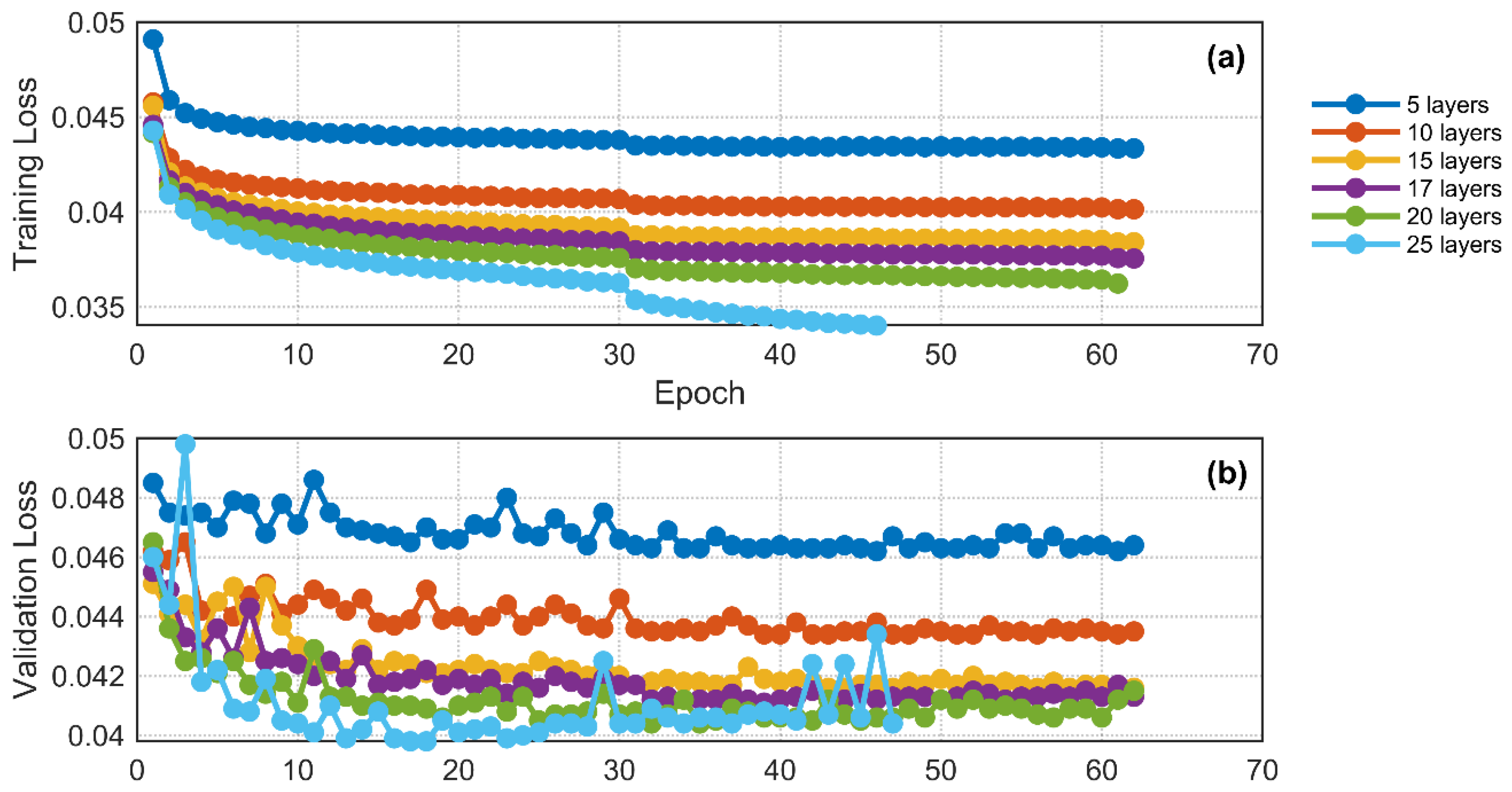
Figure 4.
Minimum validation loss obtained for DnCNN models with different depths.
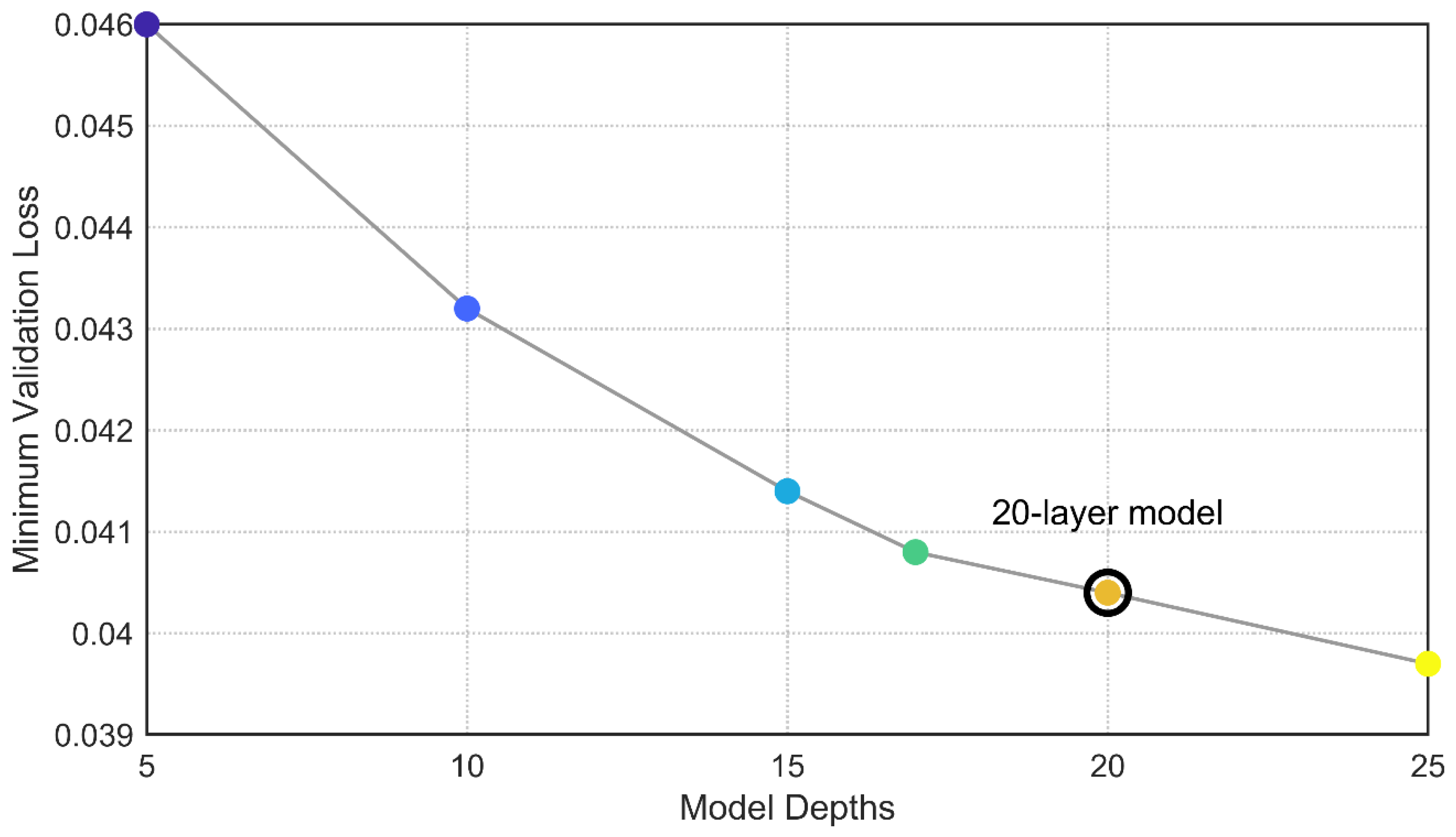
Figure 5.
Structural similarity index (SSIM) obtained from the 20-layer DnCNN model as a function of signal-to-noise ratio (SNR) for the test dataset. The heat map shows the density distribution of SSIM values across different SNR levels.
Figure 5.
Structural similarity index (SSIM) obtained from the 20-layer DnCNN model as a function of signal-to-noise ratio (SNR) for the test dataset. The heat map shows the density distribution of SSIM values across different SNR levels.
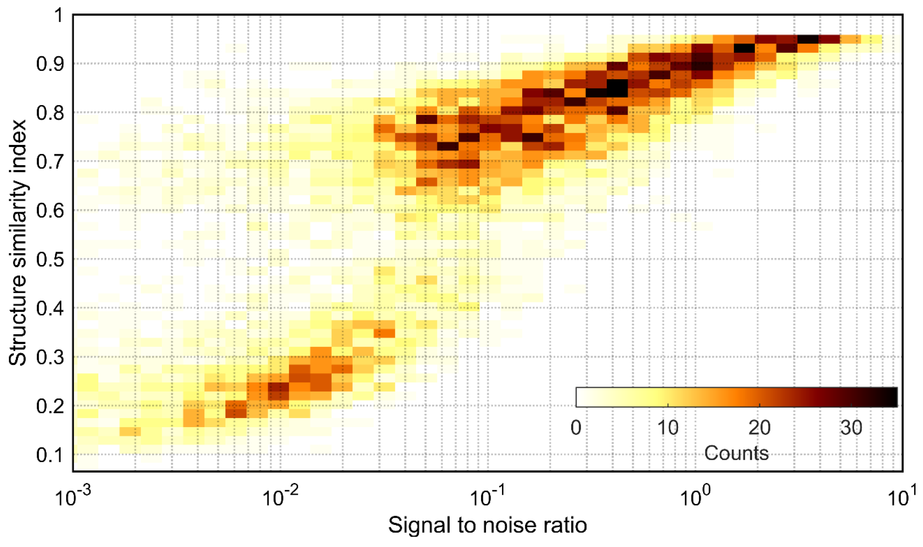
Figure 6.
Topographic relief map of the Mt. Ontake region, Japan. The inset in the upper-left corner shows the location of Mt. Ontake in a global geographic context.
Figure 6.
Topographic relief map of the Mt. Ontake region, Japan. The inset in the upper-left corner shows the location of Mt. Ontake in a global geographic context.
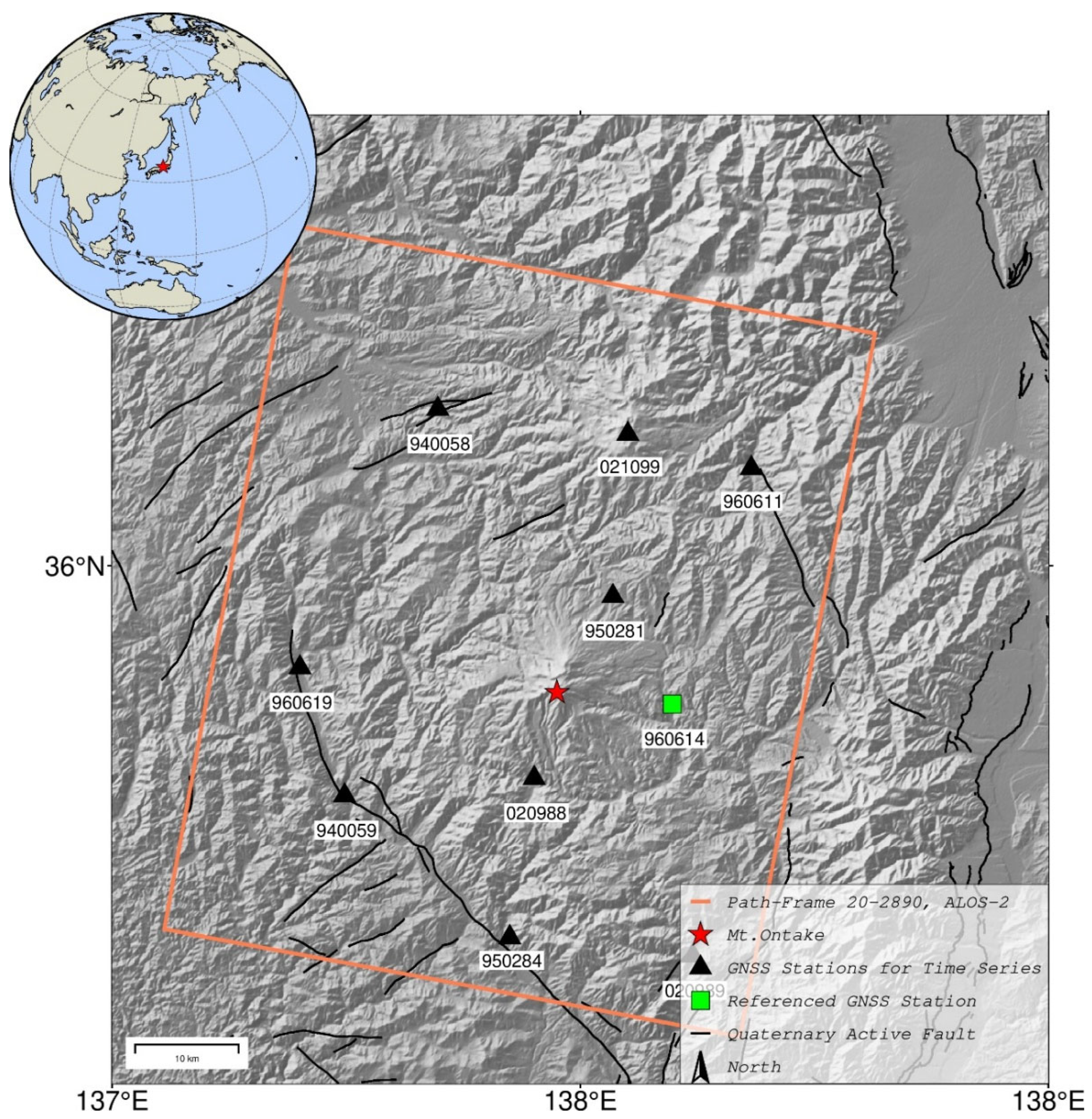
Figure 7.
Time-series deformation maps of Mt. Ontake derived from SBAS-InSAR using different atmospheric correction methods: (a) uncorrected, (b) CNN-corrected, (c) GACOS-corrected, and (d) linear-corrected results.
Figure 7.
Time-series deformation maps of Mt. Ontake derived from SBAS-InSAR using different atmospheric correction methods: (a) uncorrected, (b) CNN-corrected, (c) GACOS-corrected, and (d) linear-corrected results.
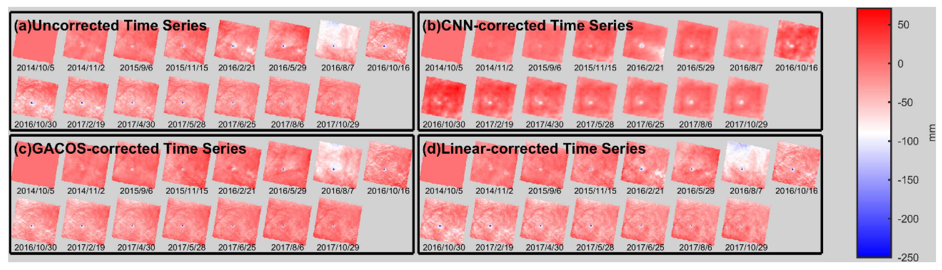
Figure 8.
Velocity fields derived from the InSAR time series using different correction methods: (a) uncorrected, (b) CNN-corrected, (c) GACOS-corrected, and (d) linear-corrected results.
Figure 8.
Velocity fields derived from the InSAR time series using different correction methods: (a) uncorrected, (b) CNN-corrected, (c) GACOS-corrected, and (d) linear-corrected results.
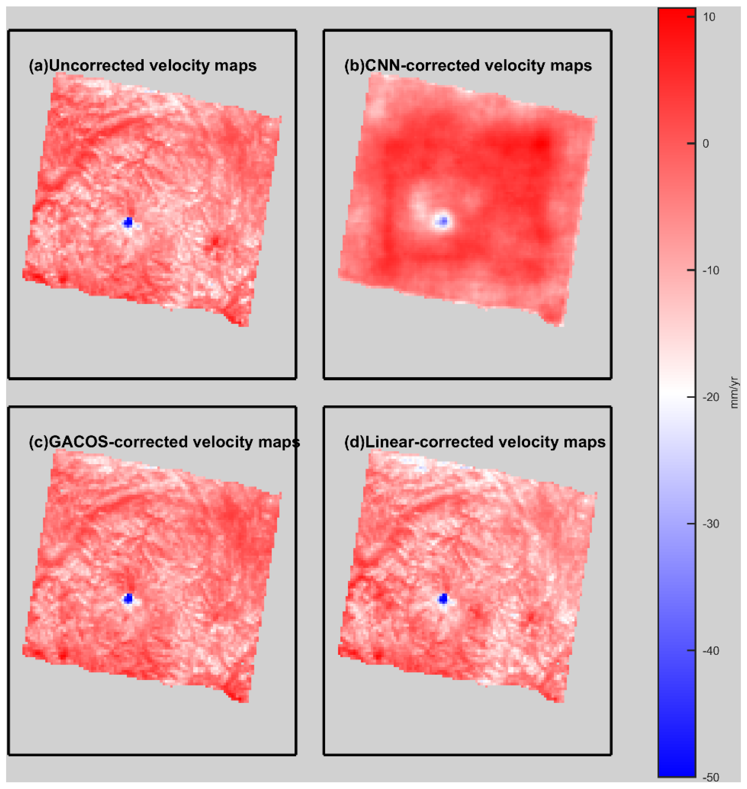
Figure 9.
Standard-error maps of the velocity fields derived using different correction methods: (a) uncorrected, (b) CNN-corrected, (c) GACOS-corrected, and (d) linear-corrected results. The CNN-corrected result exhibits the lowest overall standard error, indicating improved temporal consistency of the deformation estimates.
Figure 9.
Standard-error maps of the velocity fields derived using different correction methods: (a) uncorrected, (b) CNN-corrected, (c) GACOS-corrected, and (d) linear-corrected results. The CNN-corrected result exhibits the lowest overall standard error, indicating improved temporal consistency of the deformation estimates.
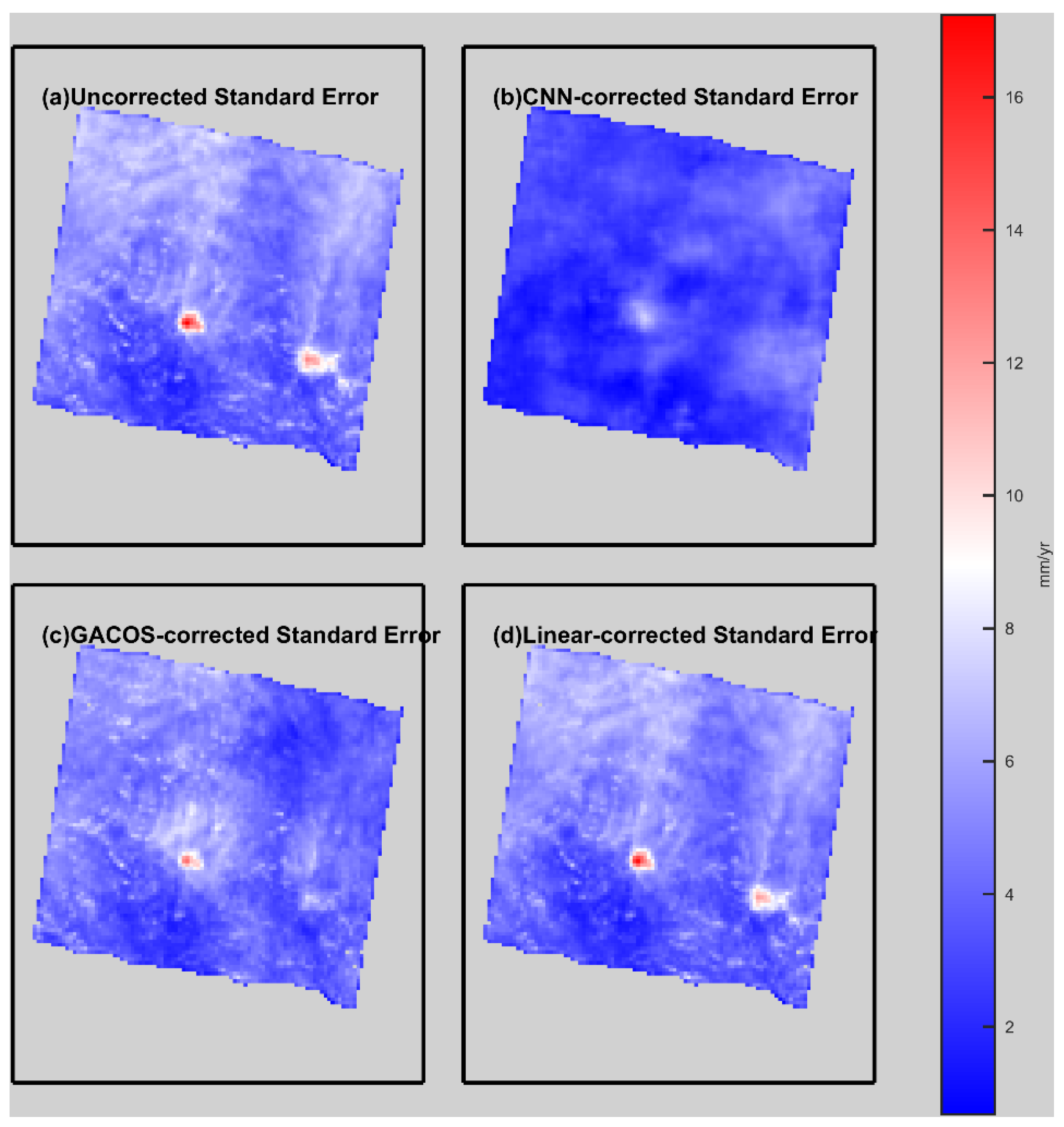
Figure 10.
LOS displacement time series at nine GNSS stations. Gray circles represent GNSS observations, while the colored lines indicate InSAR-derived LOS displacement time series from the uncorrected, CNN-corrected, GACOS-corrected, and linear-corrected datasets.
Figure 10.
LOS displacement time series at nine GNSS stations. Gray circles represent GNSS observations, while the colored lines indicate InSAR-derived LOS displacement time series from the uncorrected, CNN-corrected, GACOS-corrected, and linear-corrected datasets.
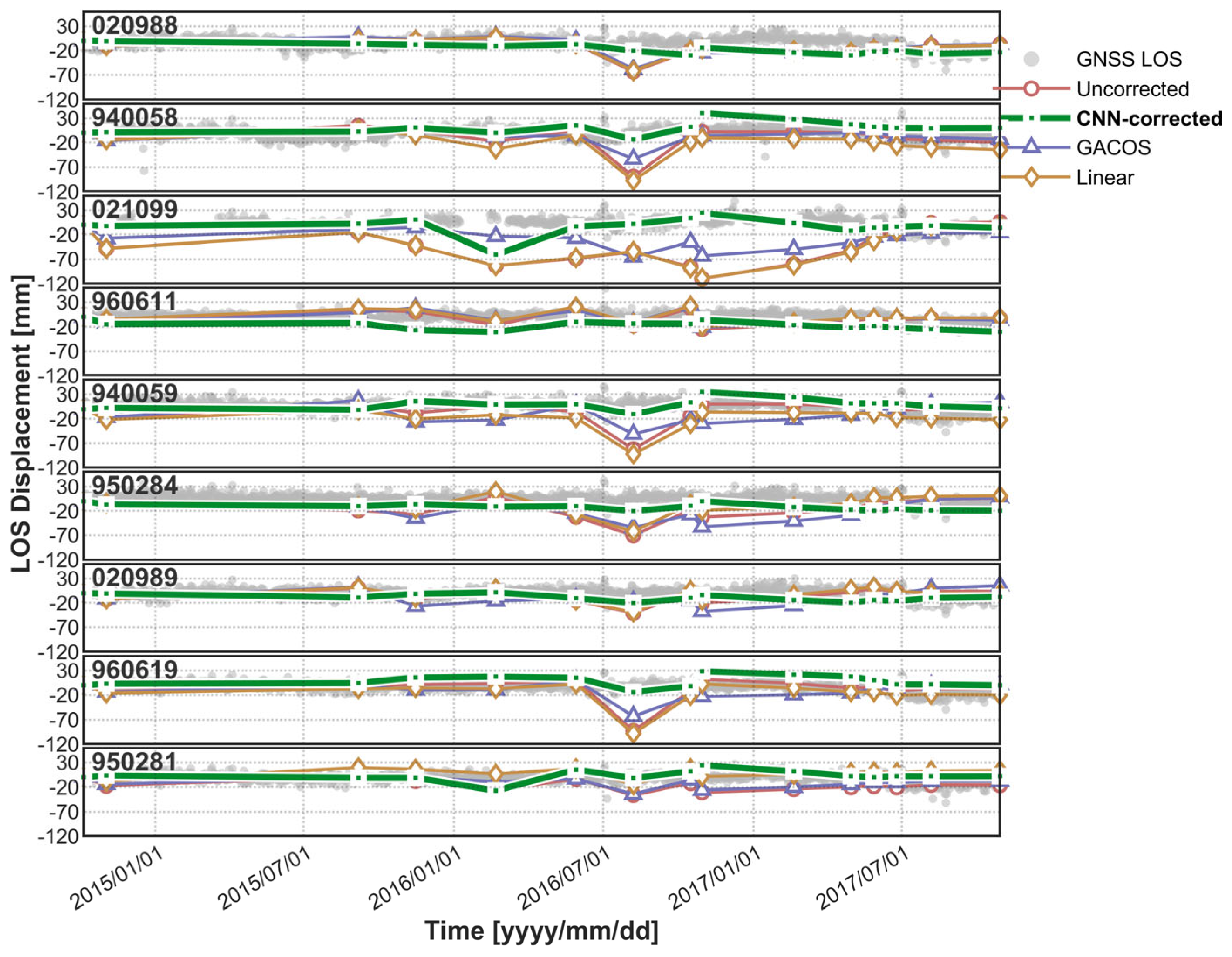
Figure 11.
Root mean square error (RMSE) between GNSS and InSAR LOS displacement time series at nine GNSS stations. Different symbols represent the uncorrected, CNN-corrected, GACOS-corrected, and linear-corrected InSAR results. Station labels are shown for reference.
Figure 11.
Root mean square error (RMSE) between GNSS and InSAR LOS displacement time series at nine GNSS stations. Different symbols represent the uncorrected, CNN-corrected, GACOS-corrected, and linear-corrected InSAR results. Station labels are shown for reference.
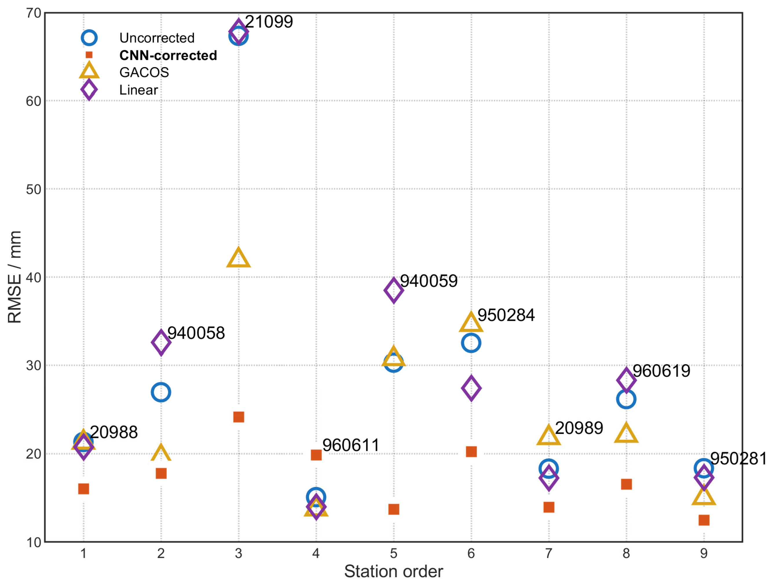
Figure 12.
Uncorrected (left) and CNN-corrected (right) coseismic deformation maps derived from an ALOS/PALSAR interferometric pair for the 2009 Mw 6.3 L’Aquila earthquake. Black triangles indicate the locations of GNSS stations used for validation, the black circle marks the earthquake epicenter, and the blue star denotes the reference station (SELL). The inset shows the geographic location of the study area in central Italy.
Figure 12.
Uncorrected (left) and CNN-corrected (right) coseismic deformation maps derived from an ALOS/PALSAR interferometric pair for the 2009 Mw 6.3 L’Aquila earthquake. Black triangles indicate the locations of GNSS stations used for validation, the black circle marks the earthquake epicenter, and the blue star denotes the reference station (SELL). The inset shows the geographic location of the study area in central Italy.
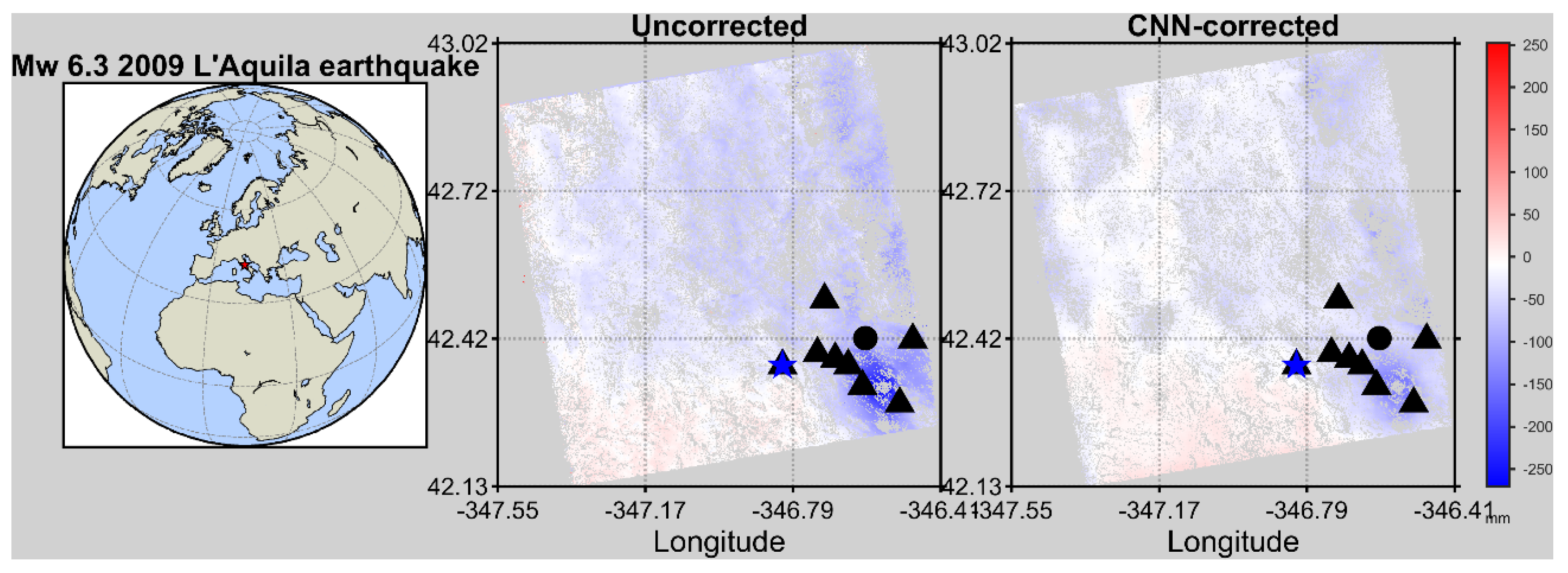
Figure 13.
Absolute differences between GNSS-derived and InSAR-derived LOS coseismic displacements at the validation stations. Blue circles represent the uncorrected InSAR results, and orange squares represent the CNN-corrected results. The CNN correction substantially reduces the discrepancy between GNSS and InSAR observations at most stations.
Figure 13.
Absolute differences between GNSS-derived and InSAR-derived LOS coseismic displacements at the validation stations. Blue circles represent the uncorrected InSAR results, and orange squares represent the CNN-corrected results. The CNN correction substantially reduces the discrepancy between GNSS and InSAR observations at most stations.
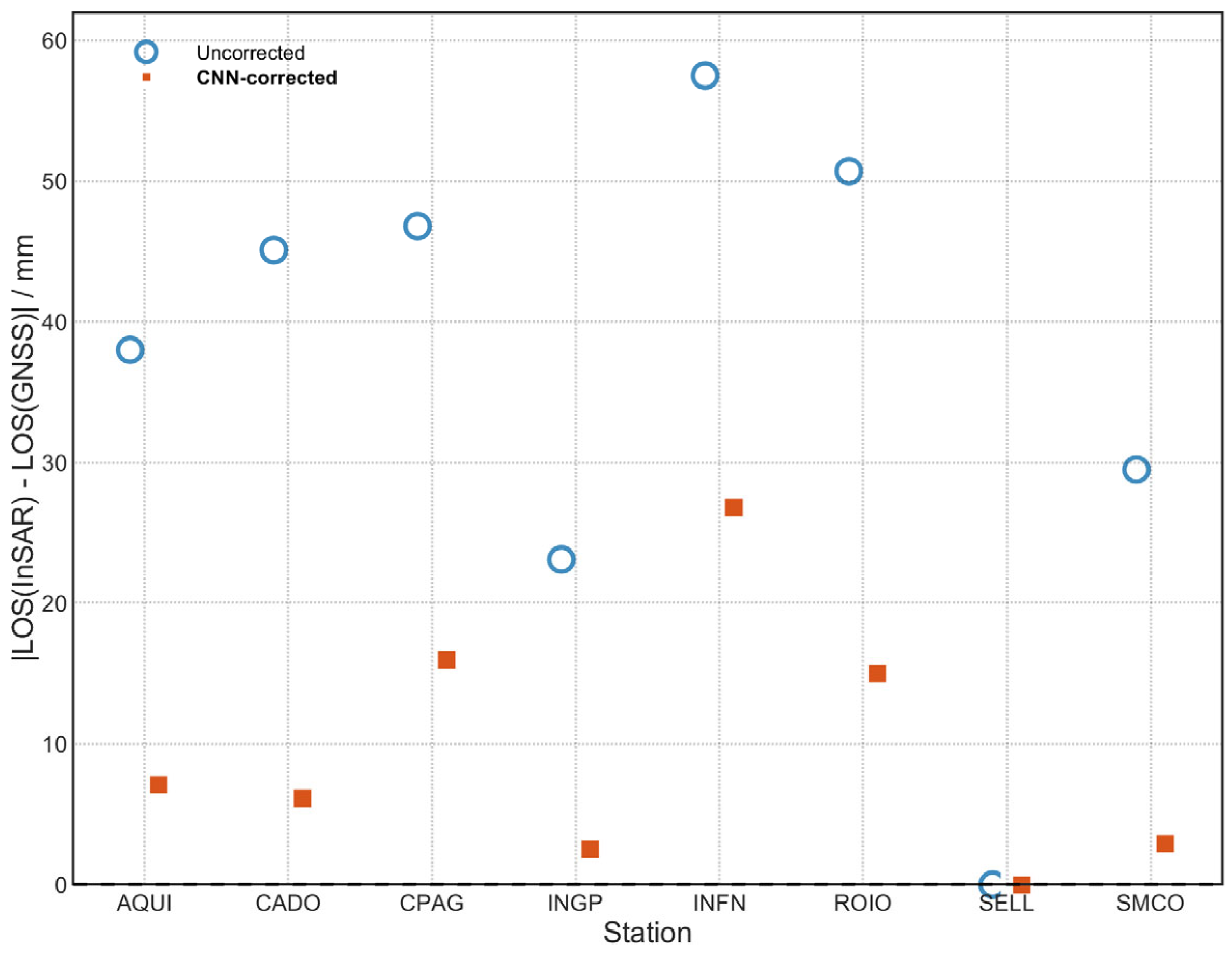
Figure 14.
Mean coherence map of the Mt. Ontake area of 59 interferograms from 20-2890. Red triangles indicate GNSS stations, and the cyan triangle denotes station 960611, which is located in an area strongly affected by low coherence. Black lines represent the Delaunay triangulation constructed from the GNSS network. Numbers indicate the mean coherence value within each triangular region.
Figure 14.
Mean coherence map of the Mt. Ontake area of 59 interferograms from 20-2890. Red triangles indicate GNSS stations, and the cyan triangle denotes station 960611, which is located in an area strongly affected by low coherence. Black lines represent the Delaunay triangulation constructed from the GNSS network. Numbers indicate the mean coherence value within each triangular region.
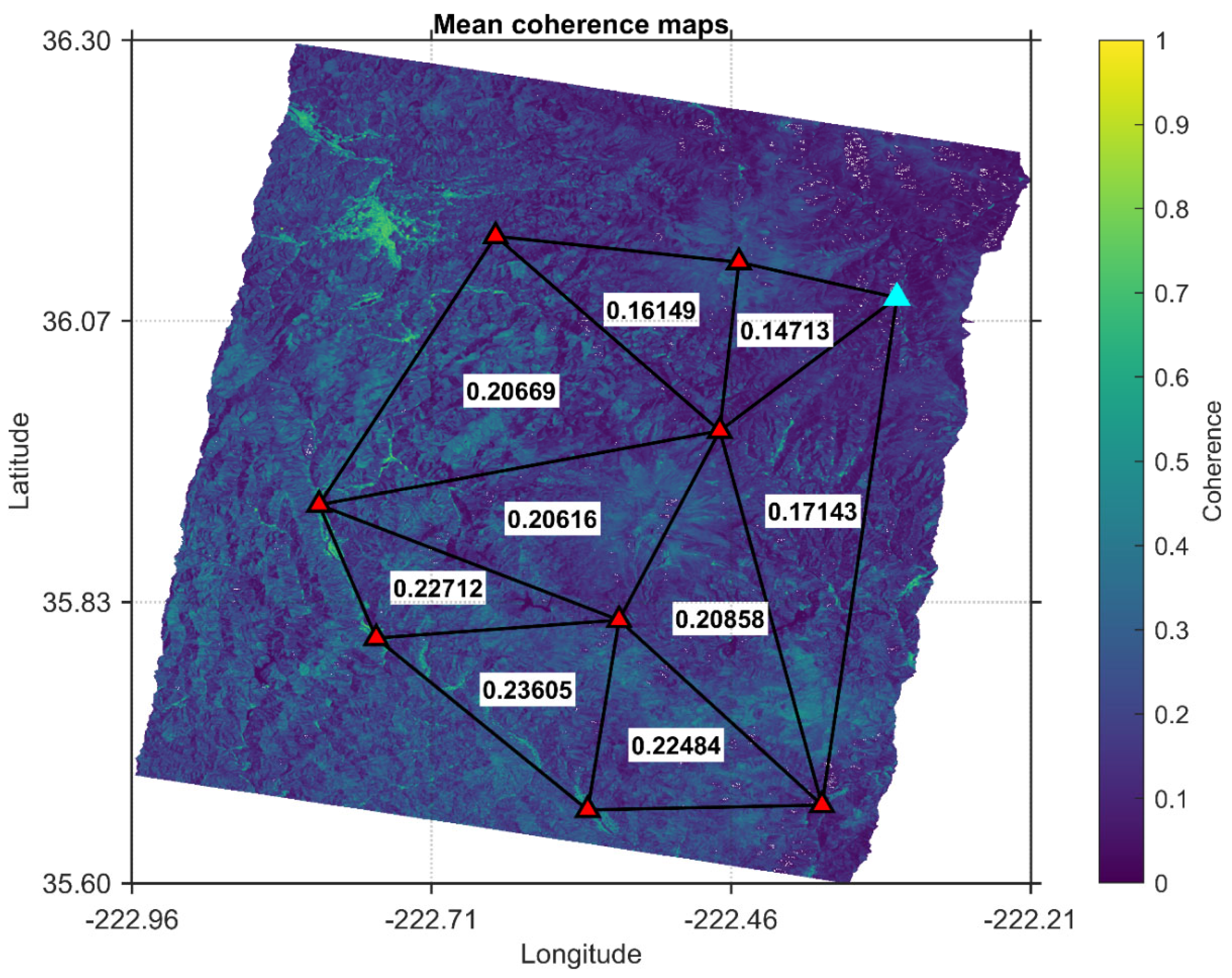

Table 1.
Summary of SAR datasets used in the Mt. Ontake and L'Aquila case studies.
| Satellite Mission/Sensor | ALOS-2/PALSAR-2 | ALOS/PALSAR |
| Orbit direction | Descending | Ascending |
| Geographic region | Mt. Ontake, Japan | L'Aquila, Italy |
| Wavelength [cm] | 22.9 | 23.62 |
| Path/Frame | 20/2890 | 639-840 |
| Date | 05.10.2014 | 21.07.2008 |
| 02.11.2014 | 22.04.2009 | |
| 06.09.2015 | ||
| 15.11.2015 | ||
| 21.02.2016 | ||
| 29.05.2016 | ||
| 07.08.2016 | ||
| 16.10.2016 | ||
| 30.10.2016 | ||
| 19.02.2017 | ||
| 30.04.2017 | ||
| 28.05.2017 | ||
| 25.06.2017 | ||
| 06.08.2017 | ||
| 29.10.2017 | ||
| Acquisition type | SLC image | Raw image |
| Polarization | HH | HH |
| Original resolution [m] | 3 | 10 |
Table 2.
Comparison of model architecture, trainable parameters, and training labels among different deep-learning approaches.
Table 2.
Comparison of model architecture, trainable parameters, and training labels among different deep-learning approaches.
| Architecture | Number of parameters [million] | Base channel | Traning label |
| DnCNN (This study) | 0.66 | 64 | Noise-based |
| Original UNet-2D | 31.03 | 64 | Signal-based |
| UNet-2D (Sun et al., 2020) | 7.76 | 32 | Signal-based |
| Autoencoder (Rouet-Leduc et al., 2021) | 0.48 | 64 | Signal-based |
Disclaimer/Publisher’s Note: The statements, opinions and data contained in all publications are solely those of the individual author(s) and contributor(s) and not of MDPI and/or the editor(s). MDPI and/or the editor(s) disclaim responsibility for any injury to people or property resulting from any ideas, methods, instructions or products referred to in the content. |
© 2026 by the authors. Licensee MDPI, Basel, Switzerland. This article is an open access article distributed under the terms and conditions of the Creative Commons Attribution (CC BY) license (http://creativecommons.org/licenses/by/4.0/).
Copyright: This open access article is published under a Creative Commons CC BY 4.0 license, which permit the free download, distribution, and reuse, provided that the author and preprint are cited in any reuse.


